Author Archives: rajani

Increasing Vigilance by Second Observer during Colonoscopy Improves Adenoma Detection Rate

DOI: 10.31038/CST.2018344

Abstract

Colon cancer is the third most common diagnosed cancer for men and women in the United States. Colonoscopy remains the best diagnostic tool for the detection of colon cancer as well as adenomatous polyps. Adenoma Detection Reate has been directly linked to prep quality, colonoscopy withdrawal time and physician feedback on competency. Recently several endoscopic devices, endoscopes and techniques have been introduced to increase individual ADR. Endoscopes that increase mucosal visualization include wide-angle colonoscopes, multiple lense colonoscopes and short turn radius colonoscopes. Accessory devices include transparent caps, endocuff, and endorings among others. Finally, these products can be augmented by having a trained technician acting as a second observer during colonoscopy. Aim: To determine if a trained technician can augment polyp detection rates as a second observer. Methods: A prospective, non-randomized, pilot study was conducted on 1681 patients undergoing surveillance colonoscopy of patients with prior history of colon polyps. Consecutive patients were performed by Standard Colonoscopy; n = 765 (m = 317, f = 448) Group I, followed by Observer Augment Colonoscopy; n = 916 (m = 392, f = 524) Group II. Data collected included prep quality (Boston Criteria), withdrawal time (WT), ADR, number of Adenomas/patient, polyp location, polyp size and advanced polyp histology. Results: ADR rates was significantly higher in Observer Augmented Colonoscopy compared to Standard Colonoscopy (41.8% vs. 37.6%, p = 0.008). Average number of polyps per patient detected by Observer Augmented Colonoscopy was 2.32/patient compared to 1.85/patient in the Standard Colonoscopy group (p = 0.001). Seventy-eight % of the augmented polyps removed were flat and 5mm or less and 42% were found in the sigmoid colon. Absolute benefit increase and Relative benefit increase was 4.2% and 11.2% respectively. No differences in prep quality or withdrawal time were observed. Conclusion: Observer Augmented Colonoscopy results in significantly higher ADR compared to Standard Colonoscopy. It also results in greater average number polyps found per individual patient most often observed in the sigmoid colon. We strongly recommend training assistants to be vigilant observers during colonoscopy. A prospective, multi-centered, randomized study is currently underway.

Keywords

Colonoscopy, Colon Cancer, Polyp, Colon Cancer Screening, Adenoma Detection Rate (ADR)

Background

Cancer is the second leading cause of death after heart diseases [1]. Colonoscopy is a widely used gold standard tool for colorectal screening and can help detect both standard and advanced colonic neoplasms in asymptomatic adults [2–6]. Several studies have demonstrated that experienced gastroenterologists miss up to 11% of advanced adenomas and 26% of all adenomas [7]. Interval colon cancer is increasingly being reported, predominately as a result of missed polyps on prior colonoscopy and reflects strongly on quality of the exam.

Removal of adenoma is considered the most effective method in reducing the incidence of mortality of CRC and warrants the success of colonoscopy as a screening procedure [3, 4, 8]. One of the benchmarks of quality colonoscopy is Adenoma Detection Rates (ADR). The ADR and Polyp Detection Rate (PDR), defined as the proportion of colonoscopies in which one or more adenomas (or polyp) are detected, are both considered as an outcomes measure for colonoscopy [5, 9]. Factors that improve polyp and adenoma detection include prolonged colonoscopy withdrawal time, improved quality of the bowel preparation, and instrument accessories such as the application of a cap-assisted colonoscopy, and the third eye retro-scope [10–14]. Recent advances have shown improved polyp detection when additional trained individuals are monitoring for polyps by concentrating on the screen throughout length of the exam [15–17]. A study done on 844 patients in Korea by Lee et al.[18] in 2011 demonstrated that endoscopy nurse participation increased ADR, however, the benefit was exclusively with inexperienced endoscopists and nurses with ≥ 2 years endoscopy experience. A randomized prospective study done at Yale University including 502 patients showed a trend toward improved overall ADR with endoscopy nurse observation during colonoscopy [19]. Nurses in this study by
Aslanian et al. 2013 had ≥ 1.5 years of prior endoscopy experience. A meta-analysis by Y.S Oh et al [20] concluded that involvement of a fellow during colonoscopy did not affect adenoma and polyp detection rates. Our aim was to further determine if observer augmented colonoscopy by an experienced endoscopy technician improves ADR versus standard colonoscopy.

Materials and Methods

We conducted a prospective, non-randomized feasibility study to determine the merits of a large scale prospective study the study was approved by institutional review board. Written informed consent for the study was obtained from all patients. A total of 1681 patients undergoing surveillance colonoscopy of patients with prior history of colon polyps were included in the study. This included 765 consecutive patients with standard colonoscopy followed by 916 patients using augmented vigilance. Those with a diagnosis of colon cancer were excluded from analysis. Bowel preparation quality, withdrawal time, ADR, number of adenomas per patient, polyp location, size and polyp histology were prospectively recorded by the endoscopist. Endoscopy technicians at each site were educated to detect polyps by monitoring the endoscopy screen throughout the exam insertion and withdrawal. Each technician had a minimum of 3 years’ experience assisting in colonoscopy. A minimum requirement for bowel preparation was Boston score of 6, with each segment having a minimal score of 2. Polyps overlooked by the endoscopist and noted by the technician were removed and the procedure was flagged for final interpretation. A missed polyp by the endoscopist was credited to the endoscopy technician upon withdrawal if no attempt was made to stop the colonoscopy to target for removal.

Results

Figure 1 shows a flow diagram of the study. In total 1681 patients were included in the study. Patients were randomized to Standard Colonoscopy (ST) n = 765 (male = 317, female = 448) Group 1, or to Observer Augmented Colonoscopy (OAC) n = 916 (male = 392, female = 524 ) Group 2.

CST 2018-119 - Wazir USA_F1

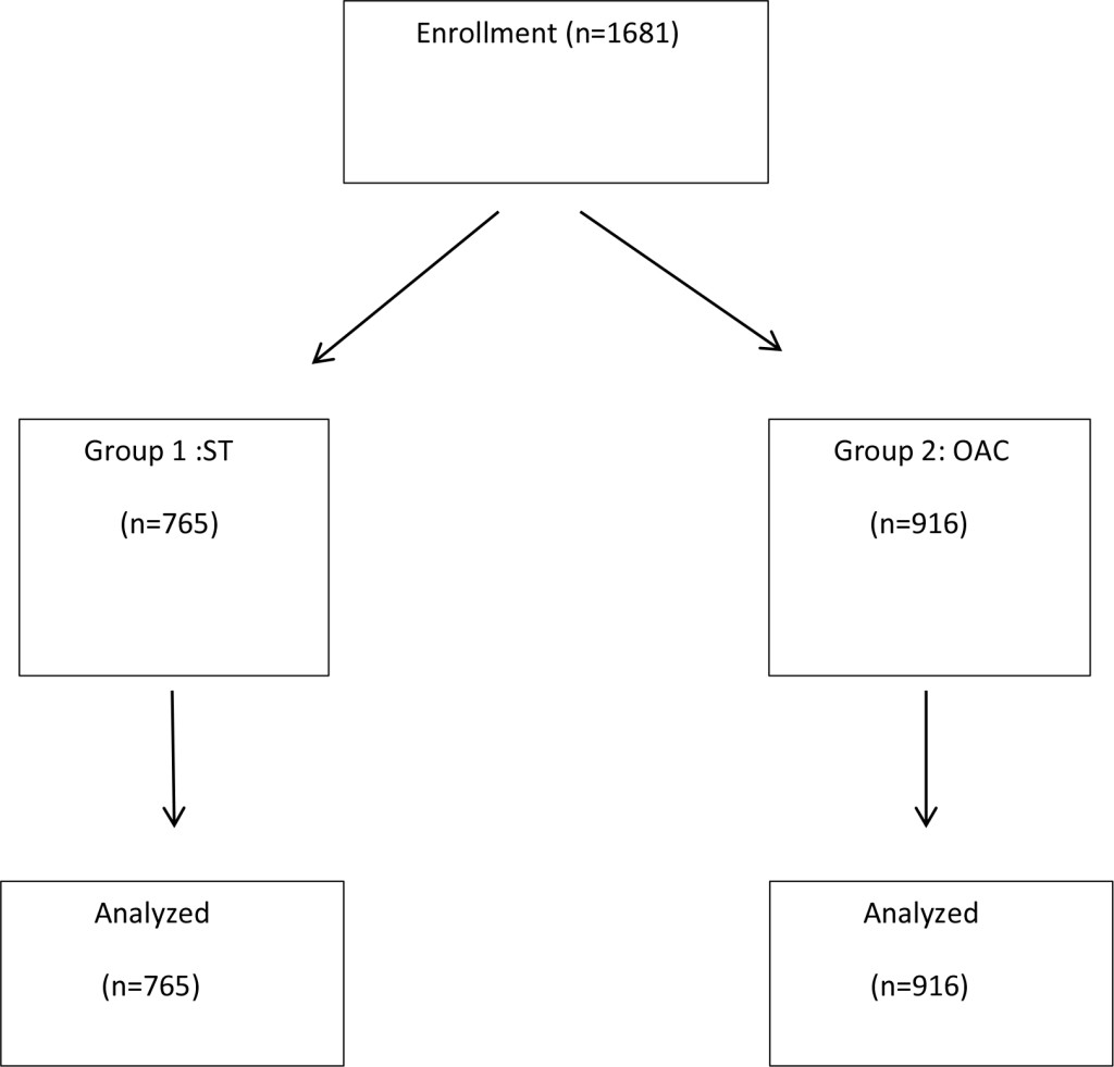
Figure 1. Schematic Diagram showing layout of the study conducted with assortment of total number of patients (n = 1681) into 2 groups. Group 1: Standard Colonoscopy (n = 765) and Group 2: Observer Augmented Colonoscopy (n = 916) and subsequent analysis.

There was no significant difference in the baseline characteristics between the two groups. 42 percent were male and 58 percent were female.

A significant difference was found in the ADR rates between the 2 groups, 41.8% in Group 2 vs 37.6% in Group 1, p = 0.008, (Table 1). Average number of polyp per patient detected by Observer Augmented Colonoscopy was 2.32/patient compared to 1.85/ patient in standard colonoscopy group (p = 0.001). Absolute Benefit Increase (ABI) was 4.2% and Relative Benefit Increase (RBI) was 11.2% with Number Needed to Treat by OAC to find one additional patient with adenoma was 23.8. Polyps less than or equal to 5 mm were found to be 73.3% in group 1 (ST) and 78% in group 2 (OAC). Polyps sized 6–9mm and equal to or more than 10 mm were 9.8% and 16.9% in group 1 and 6.4% and 15.6% in group 2 respectively. Right sided and left sided polyps were 43.7% and 56.3% in group 1 versus 35.9% and64.1% in group 2. High grade dysplasia was evident in 2.4% polyps in group 1 versus 3.9% in group 2. Cancer was detected in 0.75 and 0.79% in group 1 and group 2 respectively.

Table 1. Detection Rates of colon polyps and mean number of polyps detected per subject with percentage of polyps according the size and location

Group 1(n = 765)

Group 2 (n = 916)

p value

ADR Polyps/Pt

Polyps/pt

ABI

RBI

NNT

TOTAL POLYPS

Polyp size

1. ≤ 5mm

2. 6–9mm

3. ≥ 10mm

Polyp location

Right colon

Left colon


High grade dysplasia polyps

Cancer

 37.6%

 1.85

533

391 polyps (73.3%)

52 polyps (9.8%)

90 polyps (16.9%)

233 (43.7%)

300 (56.3%)


13 (2.4%)

04 (0.75%)

 41.8%

 2.32

889

693 polyps (78%)

57 polyps (6.4%)

139 polyps (15.6%)

319 polyps (35.9%)

570 polyps (64.1%)


35 (3.9%)

07 (0.79%)

 <0.001

 4.2%

 11.2%

 23.8

Table illustrating detection rates of colon polyps and mean number of polyps detected per subject with percentage of polyps according to side and location. Polyp/patient was higher in Group 2 at 41.8% (Observer Augmented Colonoscopy) versus 37.6% in Group 1 (Standard Colonoscopy) . Absolute Benefit Increase (ABI) was 4.2% and Relative Benefit Increase (RBI) was 11.2% with Number Needed to Treat by OAC to find one additional patient with adenoma was 23.8. Right and left sided polyps in standard colonoscopy group were 43.7% and 56.3% respectively versus 35.9% and 64.1% in augmented colonoscopy group.

Discussion

Higher ADR decreases the risk of development of colorectal cancer by finding and removing precursor lesions [5]. The recommended minimum goal of ADR is >20% in women and >30% in men [21] This may vary depending on patient population, risk factors including patient age and family history. ADR’s also are dependent on screening versus surveillance colonoscopy. As in previous studies our results show that OAC resulted in higher ADR compared to standard colonoscopy. Furthermore data showed that the average number of polyps per patient in OAC was also higher compared to standard colonoscopy and the results were statistically significant. Two previous retrospective studies have evaluated the impact of a fellow involvement during colonoscopy [16, 22].A retrospective study by Rogart et al. reported 14% improvement in the ADR by including fellows as second observers. Our results demonstrated that 82% of the augmented polyps removed were flat and 5 mm or less. In a study by Rogart et al. the adenomas detected when fellows participated were also smaller (4.4mm vs 5.8 mm, p = 0.05) from these findings it is suggested that visual scanning might be efficient when two sets of eyes are involved. In this regard our study demonstrates that trained endoscopy technician participation increases ADR significantly. Our study showed that 58% of the polyps were found in the sigmoid colon. A multicenter study [18] showed no significant difference in the anatomical location or shape of polyps.

There can be several reasons that can lead to a polyp being missed. Failure to bring the polyp into view can result in missed lesions [17]. Several potential reasons for missing adenomas during a colonoscopy include the following [23]: (a) The polyp was not detected. (b) The polyp may not be visible in field of endoscopic view due to the anatomical location. (c) The polyp was in the field of view but not recognizable. (d) The endoscopist may have been distracted. (e) The polyp was recognizable but not detected. The latter indicates that some polyps are within the field of view. The current study suggests that better recognition may be achieved by adding a second observer to improve detection of recognizable, but missed polyps. The observer can be a technician rather than a fellow or nurse. The level of fellowship training and experience also increases ADR [16]. Study by Almansa C et al. shows a relationship between visual gaze patterns (VGP) and ADR and endoscopist with higher ADR spend more time concentrating on the center of the screen [17]. By having a second set of eyes focusing on the screen it can help improve ADR by addressing potential polyp detection limitations c-e above. This essentially has the same effect as decreasing withdrawal time, more area scanned in less time. Phenomenon’s like “change blindness” when changes are missed during eye movements and interruptions in visual scanning and “inattentional blindness” when we fail to visualize something when our attention is focused elsewhere [24, 25] can be a reason for endoscopist not perceiving the presence of adenomas. In OAC some of these deficiencies can be attenuated. It is evident from our prospective study in which the ADR is 41.8% in observer augmented colonoscopy vs 37.6% in standard colonoscopy, p<0.001

Experienced endoscopy staff usually focus on performing their responsibilities, such as administering sedation under physician supervision, patient monitoring, polypectomy assistance, and other technical aspects of the procedure. All aspects of the endoscopic procedure may be facilitated by an experienced nurse and or technician. A previous retrospective study showed that an experienced nurse increased the PDR versus an inexperienced nurse [26]. In a single-center retrospective study conducted by the same investigators endoscopy nurse inexperience was associated with increased odds for immediate complications, decreased cecal intubation rates and prolonged procedure times [27]. The endoscopy nurse/technician can help improve the quality of screening colonoscopy as an additional observer. We also believe that methods for maximizing polyp detection should be a part of endoscopy nurse and technician training programs. Endoscopy technicians in our study were educated to detect polyps in the observer augmented group which they performed along with their routine responsibilities during colonoscopy. Furthermore they had a minimum of 3 years’ experience in assisting with colonoscopy and polypectomy.

Colonoscopy rarely misses polyps that are equal to or greater than 10 mm, but the miss rate increases significantly in smaller sized polyps [28, 29]. Nonpolypoid depressed adenomas are more difficult to identify during a screening colonoscopy, but they carry a greater risk for developing into high-grade dysplasia or sub mucosal invasive cancer [30, 31]. Our results showed that most of the polyps identified in dual observation group were flat and 5mm or less and more than half of them were found in the sigmoid colon. There is no record whether the endoscopy technician or the endoscopist found the polyps. Our study mirrors the study by Lee et al. [18] who reported that only 7 (7/408, 1.7%) nonpolypoid depressed adenomas were found in the dual-observation group, but they did not record whether the nurse or endoscopist found the lesions. Increasing the detection of sessile polyps has been recognized as an important factor in improving the efficacy of colonoscopy particularly in the prevention of right-sided colon cancers [32]. A study by Sawhney MS et al [33] stated that adenomas with high grade dysplasia are more likely to be flat and in the proximal colon. Total colonic dye-spray enhances the detection of small adenomas in the proximal colon and patients with multiple adenomas [34]. A randomized controlled trial also concluded that chromoendoscopy improves the total number of adenomas detected and enhances the detection of diminutive and flat lesions [35].These technologies are time-consuming and not standard of care.

Our technicians were educated to inspect the mucosa for polyps during insertion and withdrawal phases. Studies by Aslanian [19], Lee [18] and Kim [36] inspected the colonic mucosa during withdrawal phase but did not report the phase in which the inspection occurred.

Recent randomized trials with High Defination (HD) colonoscopy have reported a high ADR, ranging from 48.4% to 57% in patients with indication screening [37, 38]. High-definition chromo colonoscopy marginally increased overall adenoma detection, and yielded a modest increase in flat adenoma and small adenoma detection, compared with high-definition white light colonoscopy [38]. The high adenoma detection rates observed in this study may be due to the high-definition technology used in both groups and the fact that these were colonoscopy surveillance patients. Further prospective investigations need to be performed in this regard.

Our study had certain limitations. It was not randomized but rather a consecutive enrollment of patients, first with standard colonoscopy and subsequently with augmented colonoscopy a better study would have been randomized study using a computer to alternate colonoscopy methods. Furthermore the study was not blinded, the endoscopist knew the procedure was augmented or not and could have added bias to the results. Nonetheless our study confirms that of others that visual augmentation can uncover previously overlooked polyps. It also shows that technicians can perform as well as endoscopy nurses and or GI fellows based on previous study results.

Nurses and or technicians appear to be ideal second observers given their experience and integral involvement in procedures. The implementation of routine observation by endoscopy staff should not require a significant increase in resource utilization. Therefore we recommend that both nurses and technicians be vigilant observers during colonoscopy while refraining from other responsibilities particularly during the withdrawal phase of the colonoscopy.

References

  1. Jemal A, Siegel R, Ward E, Hao Y, Xu J, et al. (2008) Cancer statistics, 2008. CA Cancer J Clin 58: 71–96. [crossref]
  2. Lieberman DA, Weiss DG, Bond JH, Ahnen DJ, Garewal H, et al. Use of colonoscopy to screen asymptomatic adults for colorectal cancer. New England Journal of Medicine 343: 162–168.
  3. Zauber A G, Winawer SJ, O’Brien MJ (2012) “Colonoscopic polypectomy and long-term prevention of colorectal-cancer deaths,” The New England Journal of Medicine 366: 687–696.
  4. Winawer SJ, Zauber AG, Ho MN, O’Brien MJ, Gottlieb LS, et al. (1993) Prevention of colorectal cancer by colonoscopic polypectomy. The National Polyp Study Workgroup. N Engl J Med 329: 1977–1981. [crossref]
  5. Kaminski MF, Regula J, Kraszewska E et al. (2010) “Quality indicators for colonoscopy and the risk of interval cancer,” The New England Journal of Medicine 362: 1795–1803.
  6. Davila RE, Rajan E, Baron TH (2006) ASGE guideline: colorectal cancer screening and surveillance. Gastrointest Endosc 63: 546–557.
  7. Heresbach D, Barrioz T, Lapalus MG (2008) Miss rate for colorectal neoplastic polyps: a prospective multicenter study of back-to-back video colonoscopies. Endoscopy 40: 284–290.
  8. Atkin WS, Morson BC, Cuzick J (1992) Long-term risk of colorectal cancer after excision of rectosigmoid adenomas. New England Journal of Medicine 326: 658–662.
  9. Williams JE, Holub JL, Faigel DO (2012) Polypectomy rate is a valid quality measure for colonoscopy: results from a national endoscopy database. Gastrointestinal endoscopy 75: 576–582.
  10. Leufkens AM, DeMarco DC, Rastogi A (2011) “Effect of a retrograde-viewing device on adenoma detection rate during colonoscopy: the TERRACE study,” Gastrointestinal Endoscopy 73: 480–489.
  11. S. C. Ng, K. K. F. Tsoi, H. W. Hirai (2012) “The efficacy of cap-assisted colonoscopy in polyp detection and cecal intubation: a meta-analysis of randomized controlled trials,” The American Journal of Gastroenterology 107: 1165–1173.
  12. Anderson JC, Shaw RD (2014) “Update on colon cancer screening: recent advances and observations in colorectal cancer screening,” Current Gastroenterology Reports 16: 403.
  13. Overholt BF, Brooks-Belli L, Grace M, Rankin K, Harrell R, et al (2010) Withdrawal times and associated factors in colonoscopy: a quality assurance multicenter assessment. Journal of clinical gastroenterology 44: 80–86.
  14. Rex DK (2006) Maximizing detection of adenomas and cancers during colonoscopy. Am J Gastroenterol 101: 2866–2877. [crossref]
  15. Xu L, Zhang Y, Song H, Wang W, Zhang S, et al. (2016) Nurse Participation in Colonoscopy Observation versus the Colonoscopist Alone for Polyp and Adenoma Detection: A Meta-Analysis of Randomized, Controlled Trials. Gastroenterology Research and Practice 2016: 1–7.
  16. Peters SL, Hasan AG, Jacobson NB, Austin GL (2010) “Level of fellowship training increases adenoma detection rates,” Clinical Gastroenterology and Hepatology 8: 439–442.
  17. Almansa C, Shahid MW, Heckman MG, Preissler S, Wallace MB (2011) Association between visual gaze patterns and adenoma detection rate during colonoscopy: a preliminary investigation. The American journal of gastroenterology 106: 1070.
  18. Lee CK, Park DI, Lee SH, Hwangbo Y, Eun CS, et al (2011) Participation by experienced endoscopy nurses increases the detection rate of colon polyps during a screening colonoscopy: a multicenter, prospective, randomized study. Gastrointestinal endoscopy 74: 1094–1102.
  19. Aslanian HR, Shieh FK, Chan FW, Ciarleglio MM, Deng Y, et al. (2013) Nurse observation during colonoscopy increases polyp detection: a randomized prospective study. Am J Gastroenterol 108: 166–172.
  20. Oh YS, Collins CL, Virani S, Kim MS, Slicker JA, et al. (2013) “Lack of impact on polyp detection by fellow involvement during colonoscopy: a meta-analysis,” Digestive Diseases and Sciences 58: 3413–3421.
  21. Rex DK, Schoenfeld PS, Cohen J, Pike IM, Adler DG, et al. (2015) Quality indicators for colonoscopy. Gastrointestinal endoscopy 81: 31–53
  22. Rogart JN, Siddiqui UD, Jamidar PA, Aslanian HR (2008) Fellow involvement may increase adenoma detection rates during colonoscopy. The American journal of gastroenterology 103: 2841.
  23. Wallace MB (2007) Improving colorectal adenoma detection: technology or technique?. Gastroenterology 132: 1221–1223.
  24. Wolfe JM, Reinecke A, Brawn P (2006) Why don’t we see changes? The role of attentional bottlenecks and limited visual memory. Visual Cognition 14: 749–780.
  25. Simons DJ, Chabris CF (1999) Gorillas in our midst: Sustained inattentional blindness for dynamic events. Perception. 28: 1059–1074.
  26. Dellon ES, Lippmann QK, Sandler RS, Shaheen NJ (2008) Gastrointestinal endoscopy nurse experience and polyp detection during screening colonoscopy. Clin Gastroenterol Hepatol 6: 1342–1347.
  27. Dellon ES, Lippmann QK, Galanko JA, Sandler RS, Shaheen NJ (2009) Effect of GI endoscopy nurse experience on screening colonoscopy outcomes. Gastrointestinal endoscopy 70: 331–343.
  28. van Rijn JC, Reitsma JB, Stoker J, Bossuyt PM, van Deventer SJ, et al. (2006) Polyp miss rate determined by tandem colonoscopy: a systematic review. Am J Gastroenterol 101: 343–350. [crossref]
  29. Ahn SB, Han DS, Bae JH, Byun TJ, Kim JP, et al. (2012) The Miss Rate for Colorectal Adenoma Determined by Quality-Adjusted, Back-to-Back Colonoscopies. Gut Liver 6: 64–70. [crossref]
  30. Kudo SE, Lambert R, Allen JI (2008) “Nonpolypoid neoplastic lesions of the colorectal mucosa,” Gastrointestinal Endoscopy 68: 3–47.
  31. Matsuda T, Saito Y, Hotta K, Sano Y, Fujii T (2010) “Prevalence and clinicopathological features of nonpolypoid colorectal neoplasms: should we pay more attention to identifying flat and depressed lesions?” Digestive Endoscopy 22: 57–62.
  32. Hewett DG, Rex DK (2011) Miss rate of right-sided colon examination during colonoscopy defined by retroflexion: an observational study. Gastrointest Endosc74: 246–252.
  33. Sawhney MS, Dickstein J, LeClair J, Lembo C, Yee E (2015) Adenomas with high-grade dysplasia and early adenocarcinoma are more likely to be sessile in the proximal colon. Colorectal Dis 17: 682–688. [crossref]
  34. Brooker JC, Saunders BP, Shah SG, Thapar CJ, Thomas HJ, et al (2002) Total colonic dye-spray increases the detection of diminutive adenomas during routine colonoscopy: a randomized controlled trial. Gastrointestinal endoscopy 56: 333–338.
  35. Hurlstone DP, Cross SS, Slater R, Sanders DS, Brown S. Detecting diminutive colorectal lesions at colonoscopy: a randomised controlled trial of pan-colonic versus targeted chromoscopy. Gut. 53: 376–380.
  36. Kim TS, Park DI, Lee DY (2012) “Endoscopy nurse participation may increase the polyp detection rate by second-year fellows during screening colonoscopies,” Gut and Liver 6: 344–348.
  37. Rex DK, Helbig CC (2007) High yields of small and flat adenomas with high-definition colonoscopes using either white light or narrow band imaging. Gastroenterology 133: 42–47.
  38. Kahi CJ, Anderson JC, Waxman I, Kessler WR, Imperiale TF, et al (2010) High-definition chromocolonoscopy vs. high-definition white light colonoscopy for average-risk colorectal cancer screening. The American journal of gastroenterology 105: 1301.

Effect of Perilla Oil on Reducing Arteriosclerosis Risk: A Randomized Controlled Cross-Over Study

DOI: 10.31038/JCRM.2018144

Abstract

The risk of arteriosclerosis may be reduced by increasing the levels of α-linolenic acid (ALA), a omega-3 polyunsaturated fatty acid. Perilla oil contains abundant ALA. This randomized crossover clinical study of perilla oil investigated its safety and effects on the levels of ALA and lipid profile in 10 subjects. Half of the subjects took 1 tablespoon of perilla oil (ALA content = approximately 9.4 g) and the remaining half took 1 tablespoon of olive oil (ALA content = approximately 0.09 g) daily for 1 week. After a 28-day washout period, each group switched and took the other oil for 1 week. Variables were measured before and after each week of oil ingestion. The ratio of low density lipoprotein cholesterol to high density lipoprotein cholesterol significantly decreased after ingestion of perilla oil (2.7 ± 0.6 vs. 2.6 ± 0.6, P = 0.037). The levels of ALA significantly increased after ingestion of perilla oil (31.6 ± 10.32 vs. 67.93 ± 24.35 µg/mL, P = 0.001). There were no adverse effects related to perilla oil. Therefore, as a dietary supplement, perilla oil has beneficial effects on the levels of ALA and lipid profile, suggesting that it contributes to a reduction in the risk of arteriosclerosis.

Keywords

Perilla oil, Olive oil, Arteriosclerosis, Vascular endothelial function, Reactive hyperemia index

Introduction

Arteriosclerosis leads to heart and cerebrovascular diseases and is the leading cause of death worldwide. Risk factors for arteriosclerosis are diabetes (DM), hypertension, dyslipidemia, obesity, and smoking [1]. Omega – 3 polyunsaturated fatty acids have attracted attention for their prophylactic effect against various disorders, including atherosclerosis, coronary artery disease, and inflammatory diseases [2, 3]. There are reports indicating that a high intake of α-linolenic acid (ALA), a plant-derived omega – 3 polyunsaturated fatty acid, is associated with a reduced risk of arteriosclerosis [4, 5]. Perilla oil contains 50%–60% of ALA. This oil can easily be used as a daily dietary supplement. In the human body, ALA synthesizes eicosapentaenoic acid (EPA) [6]. It has been reported that EPA and docosahexaenoic acid (DHA), both omega – 3 polyunsaturated fatty acids contained in fish oil, exhibit antithrombotic and lipid-lowering actions [7, 8]. There have been few studies of perilla oil and its hypothetical effect on reducing arteriosclerosis.

ALA inhibits arteriosclerosis-associated inflammation and reduces oxidative stress, which contributes to improve vascular endothelial function [9, 10]. Reactive hyperemia index (RHI) has been reported to be useful for evaluating vascular endothelial function. Moreover, it is a good predictor of cardiovascular disease [11, 12]. Previous studies have suggested that ALA reduces diastolic blood pressure and increase serum triacylglycerol concentration [13]. Salonen, J.T et al. showed that estimated dietary intake of linolenic acid has an inverse correlation with mean resting blood pressure [14]. However, it must be noted that overdoses of ALA, EPA, and DHA may cause blood coagulation [15].

We conducted a randomized crossover clinical trial of perilla oil to evaluate its safety and effects on the levels of ALA, lipid profile and endothelial function as markers of atherosclerotic risk.

Materials and Methods

Test diets. Perilla oil, extracted from perilla seeds, was used as the study oil. A commercially available olive oil was used as a placebo control. The ALA content of the perilla oil was 62.9 g/100 g, while that of the olive oil was 0.6 g/100 g. The ALA content was measured at the Japan Food Research Laboratories (Tokyo, Japan). Both oils were given in a dose size of 1 tablespoon as a daily supplement at breakfast for 1 week. The estimated content of ALA in each dose was approximately 9.4 g in the perilla oil and 0.09 g in the olive oil.

Subjects. Ten untreated individuals (4 male and 6 female) who had at least two risk factors for arteriosclerosis (aging, first-degree hypertension, dyslipidemia, DM, obesity, and smoking) were enrolled [16]. For the purposes of this study, hypertension was defined as a systolic blood pressure of 140 to 159 mmHg or a diastolic blood pressure of 90 to 99 mmHg. Dyslipidemia was defined as a low-density lipoprotein cholesterol (LDL-C) ≧ 140 mg/dL. Diabetes was defined as a fasting blood glucose concentration ≧ 126 mg/dL, or a hemoglobin A1c (HbA1c) ≧ 6.37%. Obesity was defined as a body mass index (BMI) ≧ 25 kg/m2. Smoking was recorded as a risk factor regardless of whether it was past or present. The definition of aging was 45 years or older men and postmenopausal women. Table 1 shows the subjects’ characteristics. The study was approved by the Ethics Committee of Nanpuh Hospital, Kagoshima Kyosaikai, Public Interest Inc. Association, Japan. Clinical examinations were performed according to the principles of the Declaration of Helsinki. Written informed consent was obtained from all individuals.

Table 1. Characteristics of subjects taking perilla oil or olive oil supplements

No

Age

Sex

hypertension

dyslipidemia

diabetes

obesity

Smoking

1

55

Male

No

Yes

No

No

No

2

56

Female

No

Yes

No

No

No

3

44

Male

No

Yes

No

No

Yes

4

57

Female

Yes

Yes

No

No

No

5

59

Female

No

Yes

No

No

No

6

47

Male

No

No

No

Yes

Yes

7

50

Female

Yes

Yes

No

No

No

8

56

Female

No

No

No

Yes

No

9

42

Male

Yes

Yes

No

Yes

Yes

10

56

Female

Yes

Yes

No

Yes

No

Study design. This study was designed as a crossover method. The 10 subjects were randomly divided into two groups of 5, the first group took perilla oil daily for 1 week and the second group took olive oil. After a 28-day washout period, the groups were reversed, with the first group took olive oil daily for 1 week and the second group took perilla oil (Table 2).

Table 2. Protocol of clinical study design

1st period

WO 3 term

2nd period

Day 1

Day 2–7

Day 8

Day 9–35

Day 36

Day 37–42

Day 43

Examination

BMI 1

Blood pressure

Blood test

RHI 2

Intake

1 Body mass index (kg/m2), 2 Reactive hyperemia index (-), 3 Washout

Variables were measured before and after each 1-week period of oil ingestion. All measurements at the beginning of each period were completed on the first day of the period before the supplement was given. The measurements after each period were taken the next day of the last oil supplement.

Physical parameters were measured including blood pressure, BMI, RHI, and blood examinations. RHI, a measure of peripheral endothelial function, was assessed using peripheral arterial tonometry (EndoPAT 2000; Itamar Medical, Caesarea, Israel) according to the manufacturer’s instructions. Serum levels of aspartate and alanine aminotransferase, total protein, γ-glutamyl transferase, and C-reactive protein were determined by latex agglutination using a BM6050 analyzer (Kyowa-Medex Co., Ltd., Tokyo, Japan). Serum levels of uric acid, blood urea nitrogen, glucose, triglycerides, high density lipoprotein cholesterol (HDL-C), LDL-C, and HbA1c were measured using a BioMajesty JCA-BM6050 analyzer (JEOL Ltd., Tokyo, Japan). The white blood cell (WBC), red blood cell (RBC), and platelet counts were measured with an XE-5000 Hematology Analyzer (Sysmex, Co., Hyogo, Japan). Plasma fatty acids (lauric, myristic, myristoleic, myristoleic, palmitic, palmitoleic, stearic, oleic, linoleic, γ-linolenic, α-linolenic, arachidic, eicosenoic, eicosadienoic, 5–8-11 eicosatrienoic, dihomo-γ-linolenic, arachidonic, eicosapentaenoic, behenic, erucic, docosatetraenoic, docosapentaenoic, lignoceric, docosahexaenoic, and nervonic acids) were measured by SRL Inc (Tokyo, Japan).

Subjects were interviewed regarding their intake of the test oils and any symptoms they experienced during the study.

Statistical analysis. Measured values are expressed as means ± standard deviation. The data were assessed using a paired t-test to compare results before and after ingestion of each oil. Data were analyzed using SPSS Version 25 (IBM Co., Armonk, NY, USA). A value of P <0.05 was considered statistically significant.

Results

Physical parameters. There were no significant differences in blood pressure, BMI, or RHI before and after the week-long interventions with perilla oil or olive oil (Table 3).

Table 3. Physical parameters in subjects taking perilla oil or olive oil

Test oils

Before

After

P-value

Systolic blood pressure (mmHg)

Perilla oil

138.6 ± 17.2

139.4 ± 19.0

0.739

Olive oil

138.5 ± 12.0

135.5 ± 12.5

0.380

Diastolic blood pressure (mmHg)

Perilla oil

87.7 ± 12.6

85.4 ± 14.0

0.090

Olive oil

84.8 ± 10.7

84.0 ± 7.9

0.658

Body Mass Index (kg/m2)

Perilla oil

23.5 ± 2.7

23.6 ± 2.8

0.711

Olive oil

23.5 ± 2.9

23.4 ± 2.9

0.136

Reactive hyperemia index (-)

Perilla oil

1.59 ± 0.41

1.68 ± 0.50

0.571

Olive oil

1.57 ± 0.32

1.76 ± 0.58

0.100

Values are presented as mean ± standard deviation; n = 10.

Biochemical markers. After a week of perilla oil, the LDL-C/HDL-C ratio decreased significantly from 2.7 ± 0.6 to 2.6 ± 0.6
(P = 0.037, Fig. 1A). There was no statistically significant difference in the LDL-C / HDL-C ratio after subjects ingested olive oil (2.9 ± 0.8 before vs. 2.8 ± 0.7 after, P = 0.314, Fig. 1B). Perilla oil thus improved the LDL-C / HDL-C ratio.

PowerPoint プレゼンテーション

Figure 1. Ratios of low density lipoprotein cholesterol (LDL-C) to high density lipoprotein cholesterol (HDL-C) before and after 1 week of intake of perilla oil (A) or olive oil (B). Values are presented as mean ± standard deviation; n = 10.

With the exception of significant decrease of the platelet count after a week of olive oil, none of the other biochemical or hematologic markers differed significantly before and after either perilla oil or olive oil (Table 4).

Fatty acids. We compared the levels of ALA before and after test oil intake. Fig. 2 shows the result of the levels of ALA before and after 1 week of intake of perilla oil or olive oil, respectively. The levels of ALA increased significantly after intake of perilla oil (31.60 ± 10.32 vs. 67.93 ± 24.35 μg/mL, P = 0.001, Fig. 2A), while the levels did not change after intake of olive oil (30.52 ± 10.34 vs. 32.74 ± 21.26 μg/mL, P = 0.702, Fig. 2B).

PowerPoint プレゼンテーション

Figure 2. Levels of α-linolenic acid before and after 1 week of intake of perilla oil (A) or olive oil (B). Values are presented as mean ± standard deviation; n = 10.

The levels of EPA also increased significantly after perilla oil but not after olive oil (perilla oil: 46.88 ± 16.40 vs. 64.43 ± 31.32 μg/mL, P = 0.023, Fig. 3A; olive oil: 60.44 ± 44.62 vs. 53.90 ± 28.36 μg/mL, P = 0.598, Fig. 3B).

PowerPoint プレゼンテーション

Figure 3. Levels of Eicosapentaenoic acid before and after 1 week of intake of perilla oil (A) or olive oil (B). Values are presented as mean ± standard deviation; n = 10.

Table 4. Biochemical and hematology markers before and after ingesting perilla oil or olive oil for 1 week

Group

Before

After

P

Aspartate aminotransferase (IU/L)

Perilla oil

22.0 ± 6.5

24.0 ± 7.2

0.219

Olive oil

21.6 ± 4.9

22.5 ± 6.2

0.235

Alanine aminotransferase (IU/L)

Perilla oil

26.2 ± 15.4

27.8 ± 15.8

0.437

Olive oil

26.4 ± 15.8

26.5 ± 17.6

0.968

Total protein (g/dL)

Perilla oil

7.0 ± 0.3

7.0 ± 0.4

0.763

Olive oil

7.1 ± 0.3

7.0 ± 0. 3

0.273

γ- glutamyl transferase (IU/L)

Perilla oil

42.8 ± 31.1

42.6 ± 30.6

0.937

Olive oil

48.0 ± 38.5

47.1 ± 38.2

0.780

Uric acid (mg/dL)

Perilla oil

5.6 ± 1.7

5.6 ± 1.6

0.825

Olive oil

5.8 ± 1.6

5.9 ± 1.5

0.672

Blood urea nitrogen (mg/dL)

Perilla oil

13.3 ± 2.6

12.0 ± 1.6

0.229

Olive oil

12.6 ± 2.9

13.7 ± 3.6

0.390

Triglyceride (mg/dL)

Perilla oil

129.2 ± 71.8

137.3 ± 70.0

0.585

Olive oil

122.6 ±59.0

150.9 ± 108.7

0.306

High density lipoprotein cholesterol (HDL-C) (mg/dL)

Perilla oil

64.4 ± 12.8

65.6 ± 14.7

0.549

Olive oil

64.1 ± 14.0

62.8 ± 12.2

0.593

Low-density lipoprotein cholesterol (LDL-C) (mg/dL)

Perilla oil

171.0 ± 31.5

165.0 ± 30.5

0.400

Olive oil

174.4 ± 27.7

168.3 ± 32.8

0.147

C-reactive protein (mg/dL)

Perilla oil

0.2 ± 0.2

0.3 ± 0.6

0.569

Olive oil

0.1 ± 0.1

0.1 ± 0.1

0.835

White blood cell count (10^2/μL)

Perilla oil

55.2 ± 8.3

54.4 ± 10.8

0.741

Olive oil

53.3 ± 9.7

59.2 ± 6.8

0.050

Red blood cell count (104/μL)

Perilla oil

445.5 ± 44.9

444.4 ± 40.0

0.828

Olive oil

448.4 ± 42.1

446.7 ± 37.6

0.564

Platelet count (104/μL)

Perilla oil

26.0 ± 9.8

26.1 ± 10.1

0.628

Olive oil

27.5 ±10.7

26.3 ± 11.0

0.008*

Blood sugar (mg/dL)

Perilla oil

100.5 ± 10.5

98.5 ± 5.5

0.363

Olive oil

99.8 ± 9.3

101.1 ± 11.0

0.537

Hemoglobin A1c (%)

Perilla oil

5.4 ± 0.4

5.3 ± 0.4

0.394

Olive oil

5.3 ± 0.4

5.4 ± 0.4

0.096

Values are presented as mean ± standard deviation; n = 10.
*Significant difference in values analyzed with a paired t-test.

None of the other fatty acids differed significantly before and after intake of either oil (Table 5).

Table 5. Levels of Fatty acid before and after ingestion of perilla oil or olive oil for 1 week

Group

Before

After

P

Lauric acid (μg/mL)

Perilla oil

1.96 ± 1.21

2.37 ± 1.19

0.156

Olive oil

2.83 ± 2.18

2.80 ± 1.56

0.974

Myristic acid (μg/mL)

Perilla oil

25.65 ± 11.17

29.55 ± 14.12

0.160

Olive oil

28.21 ± 10.11

31.96 ± 18.92

0.504

Myristoleic acid (μg/mL)

Perilla oil

1.45 ± 0.68

2.04 ± 1.59

0.147

Olive oil

1.50 ± 0.62

2.48 ± 2.32

0.223

Myristoleic acid (%)

Perilla oil

0.04 ± 0.02

0.05 ± 0.04

0.153

Olive oil

0.04 ± 0.01

0.06 ± 0.06

0.283

Palmitic acid (μg/mL)

Perilla oil

806.65 ± 179.01

840.05 ± 199.55

0.271

Olive oil

817.21 ± 168.76

862.76 ± 261.01

0.522

Palmitoleic acid (μg/mL)

Perilla oil

64.77 ± 25.50

73.94 ± 39.24

0.247

Olive oil

65.75 ± 37.47

73.91 ± 33.71

0.445

Stearic acid (μg/mL)

Perilla oil

260.59 ± 41.50

274.05 ± 45.73

0.106

Olive oil

262.54 ± 43.77

276.61 ± 57.94

0.346

Oleic acid (μg/mL)

Perilla oil

740.99 ± 233.84

776.63 ± 258.10

0.503

Olive oil

718.07 ± 198.32

831.36 ± 306.45

0.219

Linoleic acid (μg/mL)

Perilla oil

1166.83 ± 146.40

1155.99 ± 115.14

0.654

Olive oil

1154.53±119.03

1169.50 ± 216.89

0.799

γ-linolenic acid (μg/mL)

Perilla oil

13.84 ± 5.74

12.25 ± 3.03

0.394

Olive oil

14.07 ± 3.57

14.31 ± 3.87

0.891

Arachidic acid (μg/mL)

Perilla oil

9.37 ± 1.53

9.59 ± 1.57

0.340

Olive oil

9.38±1.54

9.55 ± 1.57

0.623

Eicosenoic acid (μg/mL)

Perilla oil

5.35 ± 2.05

5.17±1.88

0.515

Olive oil

4.76 ± 1.32

5.78 ± 3.33

0.276

Eicosadienoic acid (μg/mL)

Perilla oil

8.89 ± 2.30

8.63 ± 2.43

0.562

Olive oil

8.48 ± 1.85

8.94±3.35

0.604

5–8–11 eicosatrienoic acid (μg/mL)

Perilla oil

3.18±0.82

2.9 ± 1.31

0.410

Olive oil

2.96 ± 1.04

3.26 ± 1.18

0.387

Dihomo-γ-linolenic acid (μg/mL)

Perilla oil

47.76 ± 9.52

44.83 ± 13.35

0.242

Olive oil

51.63 ± 21.62

51.38 ± 16.84

0.945

Arachidonic acid (μg/mL)

Perilla oil

261.62 ± 42.74

253.67 ± 50.44

0.261

Olive oil

267.28 ± 45.99

258.96 ± 44.81

0.226

Behenic acid (μg/mL)

Perilla oil

25.2 ± 5.21

25.59 ± 5.14

0.607

Olive oil

25.83 ± 4.67

25.64 ± 5.00

0.785

Erucic acid (μg/mL)

Perilla oil

1.04 ± 0.07

1.12±0.14

0.121

Olive oil

1.09 ± 0.12

1.14 ± 0.21

0.475

Docosatetraenoic acid (μg/mL)

Perilla oil

6.82 ± 1.36

6.67 ± 1.80

0.726

Olive oil

6.77 ± 1.53

7.04 ± 2.02

0.666

Docosapentaenoic acid (μg/mL)

Perilla oil

19.82 ± 5.39

22.67 ± 8.14

0.126

Olive oil

20.24 ± 5.70

19.5 ± 6.72

0.505

Lignoceric acid (μg/mL)

Perilla oil

22.14 ± 3.74

22.57 ± 4.06

0.580

Olive oil

22.68 ± 2.91

22.52 ± 3.93

0.778

Docosahexaenoic acid (μg/mL)

Perilla oil

139.94 ± 42.19

142.82 ± 48.54

0.644

Olive oil

152 ± 51.35

140.64 ± 42.32

0.134

Nervonic acid (μg/mL)

Perilla oil

42.39 ± 7.28

41.71 ± 5.64

0.641

Olive oil

43.76 ± 6.12

42.04 ± 5.86

0.197

Values are presented as mean ± standard deviation; n = 10.

Safety. There were no serious adverse events related to the intervention. There were also no significant changes in WBC, RBC, and platelet counts after ingestion of perilla oil.

Discussion

Prevention of arteriosclerosis which leads to cardiovascular disease is very important [17]. Given its apparent preventing effects, we focused our experiments on ALA and confirmed that a week’s daily intake of perilla oil significantly increased the plasma levels of ALA and EPA. It has been reported that 11% to 19% of ALA ingested from a meal is converted to EPA or DHA through an in vivo chain extension process [18]. In this study, ALA and EPA increased significantly after intake of perilla oil.. The levels of LDL-C and HDL-C were not changed after intake of perilla oil, while the LDL-C/HDL-C ratio was significantly improve. Recently, the LDL-C/HDL-C ratio has been regarded as an important index of arteriosclerosis. Even in the presence of normal levels of LDL-C, myocardial infarction may occur with low levels of HDL-C. Prevention of arteriosclerosis thus necessitates balancing the levels of LDL-C and HDL-C, which supports the concept of the LDL-C/HDL-C ratio as an important index [19, 20]. Previous study has been reported that Omega – 3 polyunsaturated fatty acids treatments reduced serum total cholesterol and LDL-C and increased HDL-C [21]. Improving of HDL-C / LDL-C ratio is important for prevention of arteriosclerosis [22]. Improving the ratio would be important to reduce arteriosclerosis risk.

No other significant differences except the changes in the LDL-C/HDL-C ratio and levels of ALA and EPA after ingestion of perilla oils were found in any of the variables we measured. There were no changes in blood pressure or BMI. Overdoses of ALA, EPA, and DHA may affect blood coagulation [15]. However, the platelet counts in our subjects did not change significantly before and after ingestion of perilla oil, and no adverse events related to blood clotting were occurred. No adverse events occurred. Therefore, the daily ingestion of perilla oil for 1 week appears to be safe.

RHI evaluates the vasodilator functions of vascular endothelium-derived vasodilators [23]. In this study, RHI was measured as an indicator of vascular endothelial function. Long-term treatment with EPA has been reported to improve impaired endothelium-dependent relaxations of atherosclerotic blood vessels [24]. In this study, we expected that the RHI might improve by perilla oil-induced increases in ALA, but there was no significant difference in the RHI before and after perilla oil.

Because ours was a short-term study with ingestion of perilla oil occurring for only 1 week and involving a small number of subjects, the study may have been underpowered to detect a significant difference in the RHI. Future studies in large numbers of individuals with long-term intake of perilla oil are needed.

Conclusion

We confirmed significant increases in the plasma levels of ALA and improvement in the LDL-C/HDL-C ratio induced by intake of perilla oil. To the extent that improvement of those markers may have a preventive effect against arteriosclerosis, our study suggests that ingestion of perilla oil may be of value in decreasing or preventing arteriosclerosis. Confirming this hypothesis will require long-term administration of perilla oil supplementation and adequate numbers of subjects so that cardiovascular outcomes can be assessed.

Acknowledgments

We are grateful to J. Saito and M. Kamiaraiso and the staff of the Department of Clinical Laboratory, Nanpuh Hospital for their tireless efforts in the carrying out this study. We also thank the study subjects for their participation.

Conflict of Interest

No potential conflicts of interest were disclosed.

References

  1. Amraoui M.E, Hjira, N. (2018) [Atypical and revelatory livedo reticularis!?]. Pan Afr Med J 29, 91.[Crossref]
  2. Connor W.E. (2000) Importance of n-3 fatty acids in health and disease. Am J Clin Nutr 71, 171S-5S. [Crossref]
  3. Takeuchi H, Sakurai C, Noda R, Sekine, S, et al. (2007) Antihypertensive effect and safety of dietary alpha-linolenic acid in subjects with high-normal blood pressure and mild hypertension. J Oleo Sci 56, 347–360. [Crossref]
  4. Lanzmann-Petithory D.(2001) Alpha-linolenic acid and cardiovascular diseases. J Nutr Health Aging 5, 179–183. [Crossref]
  5. Hu FB, Stampfer MJ, Manson JE, Rimm, EB, et al. (1999) Dietary intake of alpha-linolenic acid and risk of fatal ischemic heart disease among women. Am J Clin Nutr 69, 890–897. [Crossref]
  6. Burdge GC, Calder PC. (2005) Conversion of alpha-linolenic acid to longer-chain polyunsaturated fatty acids in human adults. Reprod Nutr Dev 45, 581–597. [Crossref]
  7. Dyerberg J, Bang H.O, Stoffersen E, Moncada S, et al. (1978) Eicosapentaenoic acid and prevention of thrombosis and atherosclerosis? Lancet 2, 117–119. [Crossref]
  8. Bonaa K.H, Bjerve K.S, Nordoy A. (1992) Habitual fish consumption, plasma phospholipid fatty acids, and serum lipids: the Tromso study. Am J Clin Nutr 55, 1126–1134. [Crossref]
  9. Han H, Yan, P, Chen L, Luo, C, et al. (2015) Flaxseed Oil Containing alpha -Linolenic Acid Ester of Plant Sterol Improved Atherosclerosis in ApoE Deficient Mice. Oxid Med Cell Longev 958217.
  10. Hong S.H, Kim M, Noh J.S, Song Y.O. (2016) Perilla Oil Reduces Fatty Streak Formation at Aortic Sinus via Attenuation of Plasma Lipids and Regulation of Nitric Oxide Synthase in ApoE KO Mice. Lipids 51, 1161–1170. [Crossref]
  11. Mudau M, Genis A, Lochner A, Strijdom H. (2012) Endothelial dysfunction: the early predictor of atherosclerosis. Cardiovasc J Afr 23, 222–231. [Crossref]
  12. Moncada S, Palmer RM, Higgs EA. (1988) The discovery of nitric oxide as the endogenous nitrovasodilator. Hypertension 12, 365–372. [Crossref]
  13. Bemelmans W.J, Muskiet F.A, Feskens E.J, Vries J.H, et al. (2000) Associations of alpha-linolenic acid and linoleic acid with risk factors for coronary heart disease. Eur J Clin Nutr 54, 865–871. [Crossref]
  14. Salonen J.T, Salonen R, Ihanainen M, Parviainen, M, et al. (1987) Vitamin C deficiency and low linolenate intake associated with elevated blood pressure: the Kuopio Ischaemic Heart Disease Risk Factor Study. J Hypertens Suppl 5, S521–4. [Crossref]
  15. von Houwelingen R, Nordoy, A, van, der Beek E, Houtsmuller U, et al. (1987) Effect of a moderate fish intake on blood pressure, bleeding time, hematology, and clinical chemistry in healthy males. Am J Clin Nutr 46, 424–436. [Crossref]
  16. Scheuner M.T. (2003) Genetic evaluation for coronary artery disease. Genet Med 5, 269–285. [Crossref]
  17. Wang Y.Z, Yang L, Li C.F. (2018) Protective effect of atorvastatin meditated by HMGCR gene on diabetic rats with atherosclerosis: An in vivo and in vitro study. Biomed Pharmacother 104, 240–251. [Crossref]
  18. Emken E.A, Adlof R.O, Gulley R.M. (1994) Dietary linoleic acid influences desaturation and acylation of deuterium-labeled linoleic and linolenic acids in young adult males. Biochim Biophys Acta 1213, 277–288. [Crossref]
  19. Yokokawa H, Yasumura S, Tanno K, Ohsawa, M, et al. (2011) Serum low-density lipoprotein to high-density lipoprotein ratio as a predictor of future acute myocardial infarction among men in a 2.7-year cohort study of a Japanese northern rural population. J Atheroscler Thromb 18, 89–98. [Crossref]
  20. Tomosugi N, Yamamoto S, Takeuchi M, Yonekura, H, et al. (2017) Effect of Collagen Tripeptide on Atherosclerosis in Healthy Humans. J Atheroscler Thromb 24, 530–538. [Crossref]
  21. Shen T, Xing G, Zhu J, Zhang, S, et al. (2017) Effects of 12-week supplementation of marine Omega-3 PUFA-based formulation Omega3Q10 in older adults with prehypertension and/or elevated blood cholesterol. Lipids Health Dis 16, 253. [Crossref]
  22. Kanaoka T, Takahashi J, Wakamatsu Y, Ishii, K, et al. (2012) Lowered postoperative ldl-c/hdl-C ratio reduces later cardiovascular events after abdominal aortic aneurysm surgery. Ann Vasc Dis 5, 36–44. [Crossref]
  23. Axtell A.L, Gomari F.A, Cooke J.P. (2010) Assessing endothelial vasodilator function with the Endo-PAT 2000. J Vis Exp. [Crossref]
  24. Tagawa H, Shimokawa H, Tagawa T, Kuroiwa-Matsumoto M, Hirooka Y, et al. (1999) Long-term treatment with eicosapentaenoic acid augments both nitric oxide-mediated and non-nitric oxide-mediated endothelium-dependent forearm vasodilatation in patients with coronary artery disease. J Cardiovasc Pharmacol 33, 633–640. [Crossref]

Construct Validity Screening Biometrics. Construct validity of the BARABAZ-scan to screen biometrics in employees

DOI: 10.31038/JCRM.2018143

Abstract

Objective Preventive screenings and services to assess and monitor health-status in employees give valuable insights for individuals and increase health-consciousness. This may influence health-related behaviour. The BARABAZ-scan is a non-invasive test that is used to screen physiological measures. This study describes the construct validity of the signals from the BARABAZ-scan compared to signals from a golden standard instrument for the variables galvanic skin response, oxygen saturation of the blood and heath rate variability.

Methods: In the spring of 2018 three consecutive measurements per subject were conducted in a private practice. The room where measurements took place was decorated quietly and calming music was played.

Results: Of all 75 participants, 56 were female. The median age of the participants was 50 (21–82) 34 years of age. GSR-scores varied between the BARABAZ-scan and Shimmer and showed a median (range) of respectively µS = 50 (19–60) and µS = 32 (3–80). A strong correlation was found on GSR- scores between both devices ρ = 0.75 (p < 0.001). Oxygen saturation showed a mode of SpO2 = 99 and ranged from SpO2 = 95 to 99 on both instruments. The correlation between the measurements was strong with a ρ = 0.97 (p < 0.001). HRV gave a median (range) score for the RR-intervals from the BARABAZ-scan and Mobi 8 of respectively 0.867 (0>618–1.163) and 0.877 (0.651–1.052) seconds, the RMSSD was calculated at 28 ± 10.8 and 28 ± 9.4. The agreement was found at ICC = 0.98.

Conclusions: Based on this research, strong correlations were found between signals from the BARABAZ-scan and the golden standard references. The measurements from the BARABAZ-scan are useful to gain insight into physiological measures within a working age population.

Keywords

physiology, biometry, employment

Background

Good health of employees is a precondition for sustainable engagement. Preventive screenings and services to assess and monitor health-status in employees give valuable insights for individuals and increase health-consciousness. This may influence health-related behaviour. When risk factors can be identified an early intervention may be prominent to prevent negative health outcomes.

The BARABAZ-scan is a non-invasive test that is used to screen body functions related to personal capacity and stress resilience criteria. Physiological measures like the electrical resistance of the skin also referred to as galvanic skin response (GSR), oxygen saturation of the blood and heart rate variability (HRV). These measures will be explained in the next paragraphs.

The Galvanic Skin Response (GSR) is defined as a change in the electrical properties of the skin as a parameter of the sweat gland function. The signal can be used to describe the function of the autonomous nervous system [1]. The electrical properties of the skin are influenced by emotions and stress. As a result of an emotional stress reaction, there is a small change in the activity of the sweat glands in the skin. As the sweat glands release sweat, small changes of the skin’s moisture change the skin and tissue conductance, which is measured by the GSR-sensor.

Recent studies show that GSR provides diagnostic information of autonomic dysfunction as well as small somatosensory nerves [2,3]. This information is particularly of interest for diabetics, patients with metabolic syndrome, and patients with micro-vascular complications [4–6]. Sudomotor dysfunction is associated with significant peripheral artery disease, vascular inflammation, and impaired glycaemic status [4–6]. Finally, an autonomic dysfunction can be used as an early detection of neuropathy in high- risk populations like diabetics. The clinical importance of GSR measurement now became ever greater, due to the diagnostic value that such a measurement can have.

Oxygen saturation (SpO2) in the blood is monitored by pulse oximetry. A pulse oximeter shines red and infrared light through a part of the body that is relatively translucent and has good arterial pulsed blood flow. The ratio of wavelengths of the red to infrared light that passes through the body part and is received by the oximeter’s detector depends on the percentage of oxygenated versus deoxygenated hemoglobin through which the light passes. The percentage of oxygen saturation thus calculated is normally greater than 95%.

This noninvasive method offers useful insights in a range of patient groups. Pulse oximetry is used for diagnosis in case of acute respiratory failure in patients with chronic obstructive pulmonary disease [7]. Furthermore, low oxygen saturation is associated with a higher risk of cognitive impairment in elderly adults [8]. Finally, pulse oximetry is commonly used in detecting sleep disorders such as apnea and hypopnea [9].

The heart rate variability (HRV) describes the changes in the time intervals between successive heartbeats. Therefore, the accurate detection of heartbeats’ timing is of crucial importance for the HRV analysis. This detection is, generally, accomplished using the ECG signal. An alternative method of measuring HRV is using blood volume pulse (BVP) signals, which seems to be a promising alternative [10]. Detecting beat-to-beat intervals (RR-intervals) using BVP is based on a principle called photopletysmography which consists of measuring the changes in volume using an optical method [11]. Changes in blood volume are caused by the change in blood pressure following every pulse. Compared with an ECG sensor, the BVP sensor can be considered more ‘user-friendly’ and less obtrusive.

The HRV is an indirect measure of the activity of the autonomous nervous system and especially the short-term measurements are suitable for ambulatory care and patient monitoring providing immediate test results [12]. A low HRV is a strong indicator of compromised health in the general population. Reduced regulatory capacity may contribute to functional gastrointestinal disorders, inflammation, and hypertension [13]. Furthermore, low HRV contributes to the prediction of all-cause mortality in prognostic modelling [14,15].

To determine the construct validity, every signal from these physiological measures retrieved from the BARABAZ-scan is compared with a golden standard measurement device. This study aims to under scribe the use of the BARABAZ-scan in daily use answering the following research question: What is the construct validity of the signals from the BARABAZ-scan compared to signals from a golden standard instrument for the variables galvanic skin response, oxygen saturation of the blood and heath rate variability?

Methods

In the spring of 2018 healthy volunteers between 18 and 67 years of age were recruited in a network of joint companies in the south of The Netherlands were invited for the study by email. One week after receiving the invitation people were called to ask for their willingness to participate. Participants were planned on one of five measurement days until a maximum of 75 study subjects was achieved. Exclusion criteria for participation were cardiovascular diseases, a pacemaker, significant skin damage, excessive sweating; metal prostheses in the fingers or limbs; pregnancy; use of medication that can affect the heartbeat. This study was approved by the Ethics Committee in Maasstad Hospital under protocol 2018–20.

Instruments

The bio-impedance sensor of the Barabaz-scan measures electrodermal activity. Besides that, the Barabaz-scan has two sensors placed on the participants’ forehead, which allows the device to measure GSR over different circuits1. A golden standard for this measure was the Shimmer 3 GSR+ which was placed on proximal part of the index- and middle finger. Measurements were taken simultaneously. This instrument was found valid in multiple research situations [16–18].

Signals from the digital pulse oximeter in the Barabaz-scan (Contec CMS 50H) are compared to the measures taken with the Onyx Vantage 9590 oximeter by Nonin. A medical device validated for clinical use and scientific research [19]. Arterial blood gas measurements, obtained by arterial puncture, remain the gold standard for measurement of oxygen saturation [20]. However, this device is able to accurately measure in challenging conditions like when people move, have dark skin pigmentation or poor peripheral blood circulation [21]. The device uses pulse-by-pulse filtering to provide precise oximetry measurements. A good accuracy (difference  < 1.5%) was shown during rest and exercise [21]. Measurements were taken straight after each other on the same index finger.

A 3-lead ECG from a TMSi Mobi 8 was used to collect data on the HRV of the participants and compare these signals with the Barabaz-scan on the RR-intervals and RMSSD. ECG sensors were placed on both clavicula and a ground electrode on the hand. The same oximeter was used on the index finger. To evaluate the correlation between the HRV parameters computed from BVP and ECG signals measures were acquired simultaneously. The ECG directly detects the R-peek, the BVP needs to be converted into a heart signal [13]. For further analysis of the ECG signal the Pan- Tompkins QRS algorithm was applied for QRS detection.

Procedure

Participants were asked not to drink alcohol or train intensively a day before the measurements, not to eat an hour before the measurements but drink sufficiently. All tests were conducted in a controlled environment following a standardized protocol. The protocol was pilot-tested and trained by all testers prior to data collection. Prior to the measurements, the study protocol was explained, and Participants subjects gave their informed consent. Measurements took place in a private practice in a quietly decorated room where calming music was played. Three consecutive measurements were conducted to secure a useful dataset. Measurements lasted two minutes, the participants didn’t speak during the measurements to minimize the chance of artifacts.

Statistical Analysis

The first dataset is being used, unless there is missing data due to possible artifacts, it that case the second or third dataset was used. Descriptive statistics are used to present baseline characteristics and collected measures. The Kolmogorov-Smirnov test showed that data is not normally distributed. Hence, Spearman’s correlation coefficient is used to test the association between instruments for GSR and oxygen saturation. The HRV was compared using intra class correlation (acceptable, 0.75- 0.89, excellent ≥ 0.9) [22]. A sample size calculation according to Bonett and Wright (2000) was performed and showed a minimum required number of 62 subjects [23]. The correlation was classified as poor (0.00 to  ± 0.25), fair ( ± 0.25 to  ± 0.50), moderate ( ± 0.50 to  ± 0.75), or strong ( ± 0.75 to  ± 1.00) [22]. All statistical analyses were performed using SPSS 24 for Windows.

Results

Of all 75 participants, 56 were female. The median age of the participants was 50 (21–82) years of age. GSR-scores varied between the BARABAZ-scan and Shimmer and showed a median (range) of respectively μS = 50 (19–60) and μS = 32 (3–80). A strong correlation was found on GSR-scores between both devices ρ = 0.75 (p < 0.001). Oxygen saturation showed a mode of SpO2 = 99 and ranged from SpO2 = 95 to 99 on both instruments. The correlation between the measurements was strong with a ρ = 0.97 (p < 0.001). HRV gave a median (range) score for the RR-intervals from the BARABAZ-scan and Mobi 8 of respectively 0.867 (0.618–1.163) and 0.877 (0.651–1.052) seconds, the RMSSD was calculated at 28 ± 10.8 and 28 ± 9.4. The agreement was found at ICC = 0.98.

Discussion

Based on this research, strong correlations were found between signals from both the BARABAZ- scan and the golden standard references. The measurements from the BARABAZ-scan are valid and therefore useful to gain insight in physiological measures within a working age population. These measures are relating to personal health status which could be a valuable way to increase sustainable engagement for organizations.

Acknowledgements

The authors of this paper would like to thank C. Posthumus en C. Gunther for their help with data collection and clinical assessment.

References

  1. Medvedev S, Belozerov A, Kluchnikov S. (2017) R&D – Clinical Evaluation Report Multiscan PRO, Model BC-OBP.
  2. Boger MS, Hulgan T, Haas DW, Mitchell V, Smith AG, Singleton JR et al (2012) Measures of small-fiber neuropathy in HIV infection. Auton Neurosci 169: 56–61. [Crossref]
  3. Thaisetthawatkul P, Fernandes JA, Herrmann DN (2013) Contribution of QSART to the diagnosis of small fiber neuropathy. Muscle Nerve 48: 883–888. [Crossref]
  4. Chahal S, Vohra K, Syngle A. (2017) Association of sudomotor function with peripheral artery disease in type 2 diabetes. Neurol Sci. 38(1): 151–156. doi: 10.1007/s10072-016-2742-3. [Crossref]
  5. Gandecka A, Araszkiewicz A, Piłaciński S, Wierusz-Wysocka B, Zozulińska-Ziółkiewicz D. (2017) Evaluation of sudomotor function in adult patients with long lasting type 1 diabetes. Polish Arch Intern Med. 127(1): 16-24. doi: 10.20452/pamw.3884. [Crossref]
  6. Zhu L, Zhao X, Zeng P, et al. (2016) Study on autonomic dysfunction and metabolic syndrome in Chinese patients. J Diabetes Investig. 7(6): 901–907. doi: 10.1111/jdi.12524. [Crossref]
  7. Amalakanti S, Pentakota MR. (2016) Pulse Oximetry Overestimates Oxygen Saturation in COPD. Respir Care. 201661(4): 423–427. doi: 10.4187/respcare.04435. [Crossref]
  8. Su LQ, Yin ZX, Xu N, Lyu YB, Luo JS, Shi XM. (2016) Association between oxygen saturation and cognitive function in older adults from longevity areas in China. Zhonghua Yu Fang Yi Xue Za Zhi. 50(7): 600–604. doi: 10.3760/CMA.J.ISSN.0253-9624.2016.07.007. [Crossref]
  9. Ricci PA, Costa FSM, Júnior ADO, et al. (2016) Journal of Respiratory and CardioVascular Physical Therapy. Vol 4. Journal of Respiratory & Cardiovascular Physical Therapy; https://periodicos.ufrn.br/ revistadefisioterapia/article/view/7933. Accessed February 19, 2018.
  10. E. Peper, R. Harvey, M. I-Mei Lin, H. Tylova, e D. Moss, (2007 )“Is There More to Blood Volume Pulse Than Heart Rate Variability, Respiratory Sinus Arrhythmia, and Cardiorespiratory Synchrony?,” Biofeedback, vol. 35, pp. 54–61.
  11. R. Haahr, 2006 “Reflectance Pulse Oximetry Sensor for the Electronic Patch,” Technical University of Denmark.
  12. Voss A, Schroeder R, Heitmann A, Peters A, Perz S. 2015 Short-term heart rate variability – Influence of gender and age in healthy subjects. PLoS One. 10(3): 1–33. doi: 10.1371/journal.pone.0118308. [Crossref]
  13. Shaffer F, McCraty R, Zerr CL. (2014) A healthy heart is not a metronome: an integrative review of the heart’s anatomy and heart rate variability. Front Psychol. 5(September): 1–19. doi: 10.3389/fpsyg.2014.01040. [Crossref]
  14. Dekker JM, Schouten EG, Klootwijk P, Pool J, Swenne CA, Kromhout D. (1997) Heart Rate Variability from Short Electrocardiographic Recordings Predicts Mortality from All Causes in Middle-aged and Elderly Men: The Zutphen Study. Am J Epidemiol. 145(10): 899–908. doi: 10.1093/oxfordjournals.aje.a009049. [Crossref]
  15. Tsuji H, Venditti FJ, Manders ES, et al. (1994) Reduced heart rate variability and mortality risk in an elderly cohort. The Framingham Heart Study. Circulation. 90(2): 878–883. doi: 10.1161/01.CIR.90.2.878. [Crossref]
  16. Chen B-R. Objective Method for Pain Detection/Diagnosis.; 2013. http://www.dtic.mil/dtic/tr/fulltext/u2/ a617259.pdf. Accessed February 9, 2018.
  17. Burns A, Doheny EP, Greene BR, et al. (2010) SHIMMERTM: An extensible platform for physiological signal capture. In: Annual International Conference of the IEEE Engineering in Medicine and Biology. IEEE; 2010: 3759–3762. doi: 10.1109/IEMBS.2010.5627535. [Crossref]
  18. Udovičić G, Ðerek J, Russo M, Sikora M. (2017) Wearable Emotion Recognition System based on GSR and PPG Signals. In: Proceedings of the 2nd International Workshop on Multimedia for Personal Health and Health Care – MMHealth ’17. New York, New York, USA: ACM Press; 53–59. doi: 10.1145/3132635.3132641.
  19. Tan A, A Citation Tan JY, Tan X, Heng J, Chua K, Foo J. (2015) Title Bench to Bed: Researchers’ Limited Awareness of Regulatory Requirements to Market Medical. Proc Int Conf Comput Electron Biomed Eng. 49–59. http://hdl.handle.net/10220/40564 http://sdiwc.net/conferences/iccebe2015/]. Accessed February 9, 2018.
  20. National Health Service (UK) Center for Evidence-based Purchasing. 2009. Project initiation document: Pulse oximeters.
  21. Lapier J, Chatellier M. (2017) Optimizing Portable Pulse Oximeter Measurement Accuracy and Consistency During Exercise. Megan J Acute Care Phys Ther. 8(3): 96–105. doi: 10.1097/JAT.0000000000000056.
  22. Portney LG, Watkins MP, Portney G WP. (2009) Foundations of Clinical Research: Applications to Practice.; doi: 10.1016/S0039-6257(02)00362-4.
  23. Bonett DG, Wright TA. (2000) Sample size requirements for estimating pearson, kendall and spearman correlations. Psychometrika. 65(1): 23–28. doi: 10.1007/BF02294183.

Clinical diversity of Low Carbohydrate Diet (LCD)

DOI: 10.31038/JCRM.2018142

Commentary

When observing the medical and health situation in the world, diabetes, obesity and metabolic syndrome have been crucial social problems in developed and also developing countries [1]. Especially, the diet therapy would be indispensable which can be continued for long years such as low carbohydrate diet (LCD) and Calorie restriction (CR). LCD was originally begun by Atkins and Bernstein before, and it has been known and popular until now. [2, 3].

After that, there was a meaningful report from Dietary Intervention Randomized Controlled Trial (DIRECT) Group that showed the predominance compared with Mediterranean and Low-Fat Diet for 2 years [4]. Successively, DIRECT group reported the results for 4 years [5]. Thus, several researchers reported the predominance of LCD for weight reduction or HbA1c value [6].

 In contrast, authors and colleagues have introduced and developed LCD in Japan for long years [7]. We have continued practice and research of LCD and activities of Japan LCD promotion association, including educational seminars, medical journals / books and presenting in medical society [8].

There has been lots of discussion about LCD and CR for years. LCD has rather superiority to CR diets and low-fat foods in the light of weight control and blood glucose variety in short period [4]. For more than 1 year or more, continuing discussion has found concerning the comparison of LCD and CR [9]. Some reports showed beneficial effect of LCD and others revealed unremarkable difference between them [6, 10, 11].

There is a prospective randomized controlled trial (RCT) that LCD of 130g /day for 6 months reduced HbA1c and BMI more than CR [12]. However, the benefit for LCD after intensive intervention has not always maintained in the light of HbA1c and BMI between LCD and CR. This study was continued and summarized one year after regarding the comparison between LCD and CR. The result showed the beneficial efficacy for the LCD on reduction of HbA1c and BMI, but improved levels did not persist compared with that of CR. However, when combined the data of both groups, HbA1c and BMI values were significantly decreased from the baseline. The superiority of LCD seemed to disappear 1 year after, but those results would suggest the comparative efficacy to improve HbA1c value at least 1 year [12].

As described above, the discussion of the clinical effect for LCD and CR has been continued for long years. However, we cannot induce the final conclusion which is superior. They are various factors involved in the evaluation and measurement of the both methods. The research has been not in vitro research or in vivo study of the same feeds to rat every day, but clinical meal study for human in their ordinary daily life.

In the primary care setting, general efficacy of LCD has been understood rather widely. On the other hand, a problem has been known about whether the LCD continuation is possible, or whether the effect of weight reduction is possible during rather long period. After a while, some patients return to their previous meal style [13]. There are some reports that the effect of LCD can be sustained rather long term [14]. Since there are various influential factors, it will be necessary to investigate related influence into detail analysis [15].

 A recent report was found that revealed several results against the previous clinical effect for LCD. There has been the Atherosclerosis Risk in Communities (ARIC) Study which has continued its research development for some decades [16]. The ARIC study has many subjects more than 430 thousand for 25 years [17]. According to the results of ARIC cohort study, they have reported a U-shaped association between the percentage of energy of carbohydrate (mean 48·9%, SD 9·4) and mortality, after calculating for multivariable adjustment. Furthermore, they calculated and compared the total carbohydrate ratio of the diet. As a result, daily meal including high (>70%) percentage or low (<40%) percentage of energy from carbohydrates were observed, in association with elevated mortality rate, and with minimal risk found between carbohydrate content ratio in 50–55% [17].

In order to evaluate the optimal intake amount of carbohydrate for the guidance recommendations associated with certain medical evidence, the protocol included the population-based study of overall carbohydrate consumption [17]. Especially, it investigated the association of carbohydrate intake amount in accordance with mortality and residual lifespan levels. As a daily meal method, LCD was applied for reducing body weight and decreasing the cardiovascular and metabolic risk. At the same time, they recommended to replace of carbohydrate food with other proteins and plant-based fats. This procedure can give the subjects practical approach for daily healthy life in the light of anti-aging medicine [17].

In the practice and research on diabetes, how should we think about the relationship between clinical matters and the Evidence-Based Medicine (EBM)? [18] EBM has not only critically examined evidence, but also considered practicality, reality and individual tastes and situations. Short-term LCD has been effective by conventional reports and may increase the motivation feeling for progressive cure and care for the patients [19]. However, on the other hand, for long-term LCD, we have to consider the required daily calorie and also carbohydrate intake amount. Based on this situation, we would like to aim for Taylor-made diet therapy according to each patient, taking account of feasibility, continuity and safety [20, 21].

 In summary, the discussion on the comparison of LCD and CR has been continued for years. The main point would be the clinical efficacy for rather long term. Each report includes each definition of LCD such as the different amount or ratio of carbohydrate in the food. Consequently, further accumulation of the data would be expected for future practice and research development.

Key words: low carbohydrate diet (LCD), Calorie restriction (CR), Dietary Intervention Randomized Controlled Trial (DIRECT), Atherosclerosis Risk in Communities (ARIC), Japanese LCD Promotion Association (JLCDPA)

References

  1. Bando H (2018) Recent problems for the elderly life – diabetes, dementia, frailty. J Diabetes Metab Disord Control. 5(5): 167‒169. DOI: 10.15406/jdmdc.2018.05.00158.
  2. Atkins RC (1981) Dr. Atkins’ diet revolution. Bantam Books, New York. ISBN-10: 0553271571, ISBN-13: 978-0553271577.
  3. Bernstein RK (1997) Dr. Bernstein’s Diabetes Solution. Little, Brown and company, New York. ISBN 10: 0316093440, ISBN 13: 9780316093446.
  4. Shai I, Schwarzfuchs D, Henkin Y, et al. (2008) Dietary Intervention Randomized Controlled Trial (DIRECT) Group. Weight Loss with a Low-Carbohydrate, Mediterranean, or Low-Fat Diet. N Engl J Med. 359: 229–241. [Crossref]
  5. Schwarzfuchs D, Golan R, Shai I (2012) Four-year follow-up after two-year dietary interventions. N Engl J Med 367: 1373–1374. doi: 10.1056/NEJMc1204792. [Crossref]
  6. Meng Y, Bai H, Wang S, Li Z, Wang Q, Chen L (2017) Efficacy of low carbohydrate diet for type 2 diabetes mellitus management: A systematic review and meta-analysis of randomized controlled trials. Diabetes Res Clin Pract. 131: 124–131. doi: 10.1016/j.diabres.2017.07.006. [Crossref]
  7. Ebe K, Ebe Y, Yokota S, Matsumoto T, Hashimoto M, Sakai Y, et al. (2004) Low Carbohydrate diet (LCD) treated for three cases as diabetic diet therapy. Kyoto Medical Association Journal 51: 125–129.
  8. Bando H, Ebe K, Muneta T, Bando M, Yonei Y (2017) Effect of low carbohydrate diet on type 2 diabetic patients and usefulness of M-value. Diabetes Res Open J. 2017; 3(1): 9–16. doi: 10.17140/DROJ-3-130.
  9. Sato J, Kanazawa A, Hatae C, Makita S, Komiya K, Shimizu T, et al. (2017) One year follow-up after a randomized controlled trial of a 130 g/day low-carbohydrate diet in patients with type 2 diabetes mellitus and poor glycemic control. PLoS One. 12 (12): e0188892. doi: 10.1371/journal.pone.0188892. eCollection 2017. [Crossref]
  10. Tay J, Luscombe-Marsh ND, Thompson CH, et al. (2015) Comparison of low- and high-carbohydrate diets for type 2 diabetes management: a randomized trial. Am J Clin Nutr 102: 780–790. [Crossref]
  11. Snorgaard O, Poulsen GM, Andersen HK, Astrup A. (2017) Systematic review and meta-analysis of dietary carbohydrate restriction in patients with type 2 diabetes. BMJ Open Diabetes Res Care 5: e000354.
  12. Sato J, Kanazawa A, Makita S, et al. (2017) A randomized controlled trial of 130 g/day low-carbohydrate diet in type 2 diabetes with poor glycemic control. Clin Nutr 36: 992–1000. [Crossref]
  13. MacLeod J, Franz MJ, Handu D, et al. (2017) Academy of Nutrition and Dietetics Nutrition Practice Guideline for Type 1 and Type 2 Diabetes in Adults: Nutrition Intervention Evidence Reviews and Recommendations. J Acad Nutr Diet 117: 1637–1658. [Crossref]
  14. Lennerz BS, Barton A, Bernstein RK, et al. (2018) Management of Type 1 Diabetes With a Very Low-Carbohydrate Diet. Pediatrics 141.
  15. Sanada M, Kabe C, Hata H, et al. (2018) Efficacy of a Moderately Low Carbohydrate Diet in a 36-Month Observational Study of Japanese Patients with Type 2 Diabetes. Nutrients 10. [Crossref]
  16. The ARIC investigators (1989) The Atherosclerosis Risk in Communities (ARIC) Study: design and objectives. American Journal of Epidemiology, 129(4), 687–702. doi: 10.1093/oxfordjournals.aje.a115184. [Crossref]
  17. Seidelmann SB, Claggett B, Cheng S, Henglin M, Shah A, et al. (2018) Dietary carbohydrate intake and mortality: a prospective cohort study and meta-analysis. Lancet Public Health. 3(9): e419-e428. doi: 10.1016/S2468-2667(18)30135-X.
  18. American Diabetes Association (2018) Lifestyle Management: Standards of Medical Care in Diabetes-2018. Diabetes Care 41: S38-S50. [Crossref]
  19. Van Horn L (2014) A diet by any other name is still about energy. JAMA 312: 900–901.
  20. Noto H, Goto A, Tsujimoto T, Noda M (2013) Low-carbohydrate diets and all-cause mortality: a systematic review and meta-analysis of observational studies. PLoS One 8: e55030. [Crossref]
  21. Dehghan M, Mente A, Zhang X, et al. (2017) Associations of fats and carbohydrate intake with cardiovascular disease and mortality in 18 countries from five continents (PURE): a prospective cohort study. Lancet 390: 2050–2062. [Crossref]

Resident and Faculty Concordance in Screening Mammography: Impact of Experience and Opportunities for Focused Instruction

DOI: 10.31038/IMCI.2018113

Abstract

Purpose: To evaluate the frequency of and reasons for patient callback from offline screening mammography, comparing residents and breast imaging faculty.

Methods: Residents and MQSA-approved fellowship-trained breast imaging faculty independently recorded prospective interpretations of a subset of bilateral clinical screening mammograms performed over a 1-year period at our NCI-designated cancer site utilizing Computer-Assisted Diagnosis (CAD). BI-RADS 1, 2, or 0 were allowed at screen interpretation. IRB-approved retrospective review compared callback performance in both groups. Descriptive statistics and multivariate logistic regression were performed.

Results: 1317 consecutive bilateral screening mammograms were reviewed. Residents recommended callback for 123/1317 (9.3%) and faculty for 110/1317 (8.4%) women (p<.0001). Overall agreement was moderate (k=0.50) with lower agreement between faculty and novices (experience < 4 weeks) (k=0.39) than between faculty and senior residents (experience > 8 weeks) (k=0.63). Agreement varied with findings: calcifications (k=0.66), mass (k=0.52), focal asymmetry (k=0.45), asymmetry (k=0.33). In multivariate regression, all four finding types were predictors of discordance: calcifications (OR 10.4, 95% CI 3.4, 33.1, p<.0001); mass (OR 19.2, 95% CI 7.7, 48.0, p<.0001); focal asymmetry (OR 21.3, 95% CI 9.9, 45.7, p<.0001); asymmetry (OR 40.1, 95% CI 21.4, 75.2, p<.0001). Odds of discordance declined by 6% with each week of resident experience (OR 0.94, 95% CI 0.89, 0.99, p=.02). Breast density was not a significant predictor.

Conclusions: Resident and faculty callback agreement was moderate but improved with resident experience. Novices often detected calcifications and masses but missed focal asymmetry and asymmetry, suggesting educational efforts should focus on the perception of asymmetry.

Introduction

Breast cancer has the second highest mortality rate of all cancers in women, and mammography is the only known screening method shown to decrease disease-related mortality [1]. Robust diagnostic performance of screening mammography is essential to this public health impact, with a delicate balance between detecting clinically significant cancers and avoiding excessive callback rates. This level of accuracy is the intended result of specialty training and years of experience in breast imaging, but the first phase is residency training [2, 3].

To meet the requirements of the Mammography Quality Standards Act (MQSA) for training in breast imaging, radiology residents spend at least 12 weeks of their 4 year training in breast imaging clinical rotations [4]. Resident evaluations are based on faculty observation of interpretative skills and procedures, patient interactions, and dictated reports. This style of individualized instruction has the potential to provide residents with personalized training. However, given the time constraints often present at busy academic centers, there is a further need for objective metrics and data that can be used to assess the performance and tailor the education of trainees in breast imaging.

As residency training is integral to mammography expertise, many previous efforts have focused on improving the training process. Previous efforts have addressed the need for varied difficulty of cases based on self- and expert-assessments to maximize the effect of training on resident performance [5]. Mathematical models have been developed in an effort to address the need for objective assessment metrics [6, 7], and some efforts have been made to identify image features predictive of error to improve the clinical utility of such models [8].

Outside of breast imaging, concordance of resident and faculty interpretation is high [9, 10]. That is not the case in breast imaging. The goal of the current study is to evaluate the frequency and morphologic reason for trainee callbacks from screening mammography and to compare them to faculty breast imager callbacks. We hypothesize that the callback rates of radiology residents will be within the national benchmarks of 8–12% but higher than those of experienced breast imaging faculty.

Materials and Methods

All cases interpreted were 2D digital four view screening mammograms obtained on GE Senographe Essential Mammography equipment (Buc, France) at one of six screening locations within one academic health system. Residents and faculty had individual workstations to view the digital studies with hard copy images available for review as desired.

Anonymized screening mammography data sheets, including resident, and faculty interpretations, were routinely recorded for Quality Assessment (QA) and educational purposes from July 1, 2014, to June 30, 2015. All the radiology residents who rotated in breast imaging took part in this process. It has been shown that trainee interpretation of screening mammography influences faculty interpretation [2]. Thus, we asked residents and faculty to fill out an initial written assessment form independently, stating whether they would recall the mammography patient for additional screening or interpret the mammogram as negative. Faculty interpretation was the reference standard for purposes of this study. Subsequent Institutional Review Board (IRBMED) approval for retrospective reviews of the data waived the need for patient consent. Data included resident weeks of training, resident observations (calcifications, mass, focal asymmetry, asymmetry), location, recommendations for a callback for additional diagnostic imaging as well as faculty observations, location, recommendation, and assessment of breast density. All eleven faculties in the breast imaging section, with nine to thirty years of experience after fellowship, were included.

The hard copy data were subsequently entered into an electronic spreadsheet by a medical student blinded to clinical outcomes (Microsoft Excel, Redmond, WA). Resident interpretation was considered concordant with faculty interpretation when the decision and reason for callback matched that of the faculty, for one breast in per breast analysis or both breasts for per patient analysis. Descriptive statistics were performed to identify data trends and distribution. Continuous variables were evaluated with means and compared using t-tests or non-parametric tests where appropriate, while categorical variables were expressed as counts or percentages and compared using chi-square tests and measures of agreement.  Kappa agreement was considered slight if <.20, fair if 0.21–0.40, moderate if 0.41–0.60, substantial if 0.61–0.80, and almost perfect if 0.81–0.99.  Logistic regression analysis was performed to evaluate predictors of resident-faculty discordance.  A stepwise forward selection algorithm was used to select covariates for multivariate logistic regression.  All statistical procedures considered p<.05 as the standard for statistical significance and were performed using SAS 9.4 (SAS Institute, Cary, NC).

Results

Data sheets were reviewed for 1,345 consecutive bilateral screening mammograms; 28 of these were excluded from further analysis because the data sheets were incomplete (n=27), or the patient had clinical symptoms that would warrant a diagnostic exam regardless of screening mammographic findings (n=1), leaving 1,317 cases. Residents recommended that 123/1,317 (9.34%) women be called back for additional imaging, while faculty recommended callbacks for 110/1,317 (8.35%) women (p<.0001). Resident and faculty callback recommendations at the per-patient level were concordant in 1208/1,317 (91.72%) cases. Residents and faculty agreed on 62 callbacks, while residents would have called back 61 women who were not called back by faculty, and faculty called back 48 women who would not have been called back by residents. Among the 62 cases of apparently concordant callbacks, the sidedness of the resident and faculty’s reasons for callback differed in 5/62 (8.07%) cases. Therefore, the true proportion of concordant interpretations on the per-patient level was 91.34%, and the remaining analysis was performed on a per-breast basis with a total sample size of 2,634.

Regarding each breast as an individual observation, the residents recommended callback in 139/2634 (5.28%) cases and the faculty in 123/2634 (4.67%) cases (p<.0001). Overall agreement between residents and faculty was moderate (k=0.50, p<.0001). Recommendations were negative concordant (no call back) in 2441/2634 (92.67%) cases, positive concordant (both call back) in 69/2634 (2.63%), resident positive/faculty negative in 70/2634 (2.66%) and resident negative/faculty positive in 54/2634 (2.05%). Types and locations of findings prompting callbacks are illustrated in Figures 1 and 2. Resident and faculty agreement were highest for calcifications (k=0.66) and lowest for asymmetry (k=0.33), presented in table 1. Agreement for location was moderate (k=0.45).

IRCI 18 - 103_F1

Figure 1. M. ammographic findings prompting recommendation for callbacks among residents and faculty, on a per breast basis.

IRCI 18 - 103_F2

Figure 2. Location of findings prompting recommendation for callbacks among residents and faculty, on a per breast basis

Table 1. Agreement between residents and faculty on type and location of findings prompting recommendation for callback from screening mammography, on a per breast basis. P-values < .05 indicate the presence of a non-zero correlation between faculty and trainee interpretations of each feature.

Cohen’s kappa

p value

 Calcifications

0.66

<.0001

 Mass

0.52

<.0001

 Focal asymmetry

0.45

<.0001

 Asymmetry

0.33

<.0001

 Location

0.45

<.0001

Breast composition was classified by faculty in 2035 cases, by ACR BI-RADS v.5 (ACR 2013). 322/2035 (15.82%) were almost entirely fatty (A); 961/2035 (47.22%) had scattered areas of fibro glandular density (B); 690/2035 (33.90%) were heterogeneously dense (C); and 62/2035 (3.06%) were extremely dense (D).

1054/2634 (40.02%) of cases were read by a first-year radiology resident, 542/2634 (20.58%) by a second-year resident, 30/2634 (1.14%) by a third-year resident, and 1008/2634 (38.27%) by a fourth-year resident. Residents had 0–15 weeks (mean 6.11 ± 3.96 weeks) of prior experience in breast imaging.

Univariate logistic regression analysis was performed to evaluate whether any of the following features was a significant predictor of resident-faculty discordance: any of the four major types of findings (as judged by faculty), the presence of moderately (Classifications C+D vs. A+B) or extremely (Classification D vs. A+B+C) dense breasts, or the duration of the resident’s breast imaging experience. These results are presented in table 2.

Table 2. Parameter estimates from univariate logistic regression predicting resident-faculty callback discordance.

Outcome: Discordance

Odds ratio

95% CI

p value

Calcifications

6.94

2.21, 21.83

<.001

Mass

13.24

5.38, 32.59

<.0001

Focal asymmetry

14.05

6.66, 29.65

<.0001

Asymmetry

28.55

15.56, 52.40

<.0001

Moderately dense breasts

1.45

1.00, 2.11

0.05

Extremely dense breasts

0.67

0.16, 2.77

0.58

Resident experience (unit = 1 week)

0.96

0.91, 1.00

0.09

Multivariate logistic regression of all factors was performed using stepwise forward selection, and all four types of findings, as well as resident experience, were retained as significant predictors. The purpose of multivariate regression is to control for other factors that may alter the odds ratio estimates of each parameter. Parameter estimates are presented in Table 3.

Discussion

Our retrospective analysis of resident and faculty callbacks in 1345 screening mammograms demonstrated moderate agreement (k=0.50) between residents and faculty. Residents recommended callback more frequently than faculty (9.34% vs. 8.35% of women, p<.0001). Radiology residents are aware of the national benchmark for screening breast mammography callbacks, which could explain the low rate. Agreement improved with resident experience so that the odds of discordance dropped by 6% for every week of resident experience in multivariate analysis. All four major types of findings prompting callbacks were associated with discordance. The Kappa agreement was highest for the presence of calcifications (k=0.66) and lowest for asymmetry (k=0.33) with the higher concordance for the presence of calcifications possibly related to presence of coronary artery disease. Likewise, the odds ratios for discordance ranged from 10.39 (95% CI 3.27, 33.08, p<.0001) for calcifications to 40.10 (95% CI 21.38, 75.21, p<.0001) for asymmetry. Breast density was not a significant predictor of discordance.

Table 3. Parameter estimates from multivariate logistic regression predicting resident-faculty discordance.

Outcome: Discordance

Odds ratio

95% CI

p value

Calcifications

10.39

3.27, 33.08

<.0001

Mass

19.23

7.71, 47.96

<.0001

Focal asymmetry

21.31

9.92, 45.74

<.0001

Asymmetry

40.10

21.38, 75.21

<.0001

Resident weeks of experience (unit = 1week)

0.94

0.89, 0.99

0.02

C statistic

0.70

Benchmark Comparison

In the highly regulated and monitored world of screening mammography, recall rate is a performance metric that has been included in most accreditation guidelines. It is easy to obtain and has been used to assess institutional and personal professional quality. In our study, recall rate is defined as the number of screening studies with a final recommendation of BI-RADS 0 (Incomplete: needs additional imaging evaluation) out of the entire screening pool.

The 2017 update to the Breast Cancer Surveillance Consortium (BCSC) benchmarks for screening mammography is essential because it reflects modern technology and practice methods. In this study, only 59% of the radiologists studied fell within the national benchmark recall range of 5–12% with a trend towards higher recall rates [11]. The National Mammography Database (NMD) is a mammography data registry also providing performance metrics for clinical practice [12] that reported a mean recall rate of 10% from the NMD with a range of 8–11.4% based on practice location and type (using comparable BI-RADS 4 recall inclusion definition). The mean recall rate in an academic setting was 9.8%.

Our data show that the recall rates for the faculty (8.35%) and residents (9.34%) both fall within the benchmark ranges by national and academic center standards. As a QA measure, this is important and timely as this is a potential metric proposed by the Physician Quality Reporting System (PQRS) by the Centers for Medicare and Medicaid Services to determine payment for services [12]. [13] performed a reader study to assess the accuracy of interpretation of screening mammograms, concluding that diagnostic volume was not the only contributor to performance. Instead, they posited a multifactorial process that they could not yet fully define. Thus, the difference in recall rate between faculty and residents in the current study is unlikely to arise from differences in interpretation volume alone.

Discordancy Rates

In the literature, interest in the concordance of radiology resident image interpretation compared to faculty interpretation has focused on residents’ on-call interpretations.

Discordance has been shown to vary depending on the complexity of imaging. MRI cases, followed by CT, are the most common sources of discordant resident interpretations. Next, plain radiographs are the third most likely image type to be associated with discordance, followed by ultrasound, a modality where residents may be helped by experienced technologists [10, 14].

Discordance on call has been shown to decrease as residents progress in their training, presumably because resident knowledge and skill improve with clinical experience and didactics [14]. However, it has been shown that subspecialist breast imagers detect more cancers (and more early-stage cancers) and have lower recall rates than general radiologists [15]. Towards the end of their training, radiology residents are largely comparable to novice general radiologists. In agreement with Lewis et al, we found that residents with more breast imaging experience were more concordant with breast imaging subspecialty faculty [7] It is likely that the subtler finding of mammographic asymmetry, which was associated with the largest odds of discordance, requires more experience for reliable detection than a discrete finding like calcifications.

Limitations

This retrospective study is subject to several limitations. First, the data collection method does not allow for the identification of the resident or faculty, so it is not possible to control for the intrinsic correlation between multiple readings by the same person. Instead, each mammographic interpretation is treated as an independent observation, which could impact both confidence intervals and overall statistical inference. Otherwise stated, a specific radiologist’s tendency to overcall or under call may be a more powerful predictor than his or her level of training or the patient’s breast density, but we are unable to test for this. Second, patient age was not included on the data sheets but could have been a factor affecting clinical interpretations either consciously or unconsciously. Third, the experience level of the faculty was not noted on the data collection sheets, but given that all of the faculty involved were at least nine years out of training, this is considered to be a minor issue. Finally, the anonymized data collection method does not enable linkage of the screening mammogram to the results of any subsequent diagnostic workup, so the clinical significance of any resident-faculty discordance remains unknown.

Conclusion

We compared frequency and rationale for callbacks from offline screening mammography between residents and breast imaging faculty and found that while resident and faculty callback agreement was only moderate, it improved with resident experience. While novices often detected calcifications and masses, concordance was low for the more subtle findings of asymmetry, suggesting educational efforts should increase emphasis on the perception of asymmetry.

References

  1. U.S. Department of Health and Human Services, Centers for Disease Control and Prevention (CDC) and the National Cancer Institute (NCI) (2015) 1999–2013 Cancer Incidence and Mortality Data. Available from: https://nccd.cdc.gov/uscs/.
  2. Hawley JR, Taylor CR, Cubbison AM, Erdal BS, Yildiz VO, et al. (2016) Influences of Radiology Trainees on Screening Mammography Interpretation. J Am Coll Radiol 13: 554–561. [crossref]
  3. Poot JD, Chetlen AL (2016) A Simulation Screening Mammography Module Created for Instruction and Assessment: Radiology Residents vs National Benchmarks. Acad Radiol. 23: 1454–1462.
  4. Sickles EA, Philpotts LE, Parkinson BT, Monticciolo DL, Lvoff NM, Ikeda DM, et al. (2006) American College Of Radiology/Society of Breast Imaging curriculum for resident and fellow education in breast imaging. J Am Coll Radiol. 3: 879–884.
  5. Grimm LJ, Kuzmiak CM, Ghate SV, Yoon SC, Mazurowski MA (2014) Radiology resident mammography training: interpretation difficulty and error-making patterns. Acad Radiol. 21: 888–892.
  6. Wang M, Wang M, Grimm LJ, Mazurowski MA (2016) A computer vision-based algorithm to predict false positive errors in radiology trainees when interpreting digital breast tomosynthesis cases. Expert Systems with Applications 64: 490–499.
  7. Lewis PJ1, Rooney TB2, Frazee TE2, Poplack SP3 (2018) Assessing Resident Performance in Screening Mammography: Development of a Quantitative Algorithm. Acad Radiol 25: 659–664. [crossref]
  8. Grimm LJ, Ghate SV, Yoon SC, Kuzmiak CM, Kim C, et al. (2014) Predicting error in detecting mammographic masses among radiology trainees using statistical models based on BI-RADS features. Med Phys 41: 031909. [crossref]
  9. Xiong L, Trout AT, Bailey JE, Brown RKJ, Kelly AM (2011) Comparison of Discrepancy Rates in Resident and Faculty Interpretations of On-Call PE CT and V/Q Scans: Is One Study More Reliable During Off Hours? Journal of the American College of Radiology 8: 415–421.
  10. Ruma J, Klein KA, Chong S, Wesolowski J, Kazerooni EA, et al (2011) Cross-sectional examination interpretation discrepancies between on-call diagnostic radiology residents and subspecialty faculty radiologists: analysis by imaging modality and subspecialty. J Am Coll Radiol 8: 409–414.
  11. Lehman CD, Arao RF, Sprague BL, Lee JM, Buist DS, Kerlikowske K, et al (2017) National Performance Benchmarks for Modern Screening Digital Mammography: Update from the Breast Cancer Surveillance Consortium. Radiology 283: 49–58.
  12. Lee CS, Bhargavan-Chatfield M, Burnside ES, Nagy P, Sickles EA (2016) the National Mammography Database: Preliminary Data. AJR Am J Roentgenol 206: 883–890. [crossref]
  13. Beam CA, Conant EF, Sickles EA (2003) Association of volume and volume-independent factors with accuracy in screening mammogram interpretation. J Natl Cancer Inst 95: 282–290. [crossref]
  14. Weinberg BD, Richter MD, Champine JG, Morriss MC, Browning T (2015) Radiology resident preliminary reporting in an independent call environment: multiyear assessment of volume, timeliness, and accuracy. J Am Coll Radiol 12: 95–100.
  15. Sickles EA, Wolverton DE, Dee KE (2002) Performance parameters for screening and diagnostic mammography: specialist and general radiologists. Radiology 224: 861–869. [crossref]

Appendix

Location_____________ Radiology Residency Year_______________ No. week’s experience__________

Screener

Resident  negative

Resident Callback

1=Ca++

2=Mass

3=Focal Asymmetry

4=Asymmetry

5=Diagnostic

Location


1=UOQ

2=LOQ

3=UIQ

4=LIQ

5=RetroA

6=DNK

Faculty negative

Faculty Callback

1=Ca++

2=Mass

3=Focal Asymmetry

4=Asymmetry

5=Diagnostic

Location


1=UOQ

2=LOQ

3=UIQ

4=LIQ

5=RetroA

6=DNK

IF BOTH CALLBACK WAS IT FOR THE SAME REASON?

Density


1=Fatty

2=Scattered

3=Hetero-

Dense

4=Extreme

Dense

1    R

      L

2    R

      L

3    R

      L

4    R

      L

5    R

      L

Comments_______________________________________________________________________________________

LOCATION

NUMBER

Upper outer Quadrant

1

Upper Inner Quadrant

2

Lower Outer Quadrant

3

Lower Inner Quadrant

4

Retroareolar

5

*DNK

6

*Do Not Know because only seen on one view

CALL BACK REASON

NUMBER

Ca++

1

Mass

2

Focal Asymmetry

3

Asymmetry

4

Architectural Distortion

5

Diagnostic Reason

6

Evaluation of use of a 0.9% sodium chloride nasal spray immediately after septoplasty and turbinectomy postoperative and its impact on patients’ quality of life

DOI: 10.31038/SRR.2018115

Abstract

Introduction: septoplasty and turbinectomy are one of the most frequently performed surgical procedures in otolaryngology, with reduced morbidity and mortality. It is known that the use of nasal saline solution increases the nasal mucociliary clearance, reducing the accumulation of secretion. However, despite being widely used, studies evaluating its efficacy in septoplasty and lower turbinectomy postoperative are still lacking.

Objective: To prove the benefit of Maresis (0.9% isotonic solution spray) in septoplasty and lower turbinectomy postoperative.

Method: Randomized, parallel, controlled, single-blind, single-center study, held at the IPO (Instituto Paranaense de Otorrinolaringologia), in which 106 patients underwent septoplasty and bilateral lower turbinectomy, divided into 2 groups (with and without application of Maresis) and compared objectively regarding the improvement in breathing, degree of mucosal edema, crusting and ease of crusts removal in the third and tenth day after surgery. Subjective evaluation regarding the obstruction, crusting and difficulty to sleep was also performed.

Results: The product shows a statistically significant result regarding the parameter ease of crusts removal and improved quality of sleep. Statistically significant differences for mucosal edema reduction and crusting were not observed between the two groups.

Conclusion: the use of Maresis® as an adjuvant in the treatment of immediate septoplasty and bilateral lower turbinectomy postoperative assists in the process of crusts removal and improving the quality of sleep in postoperative.

Key words

nasal spray. septoplasty. turbinectomy. post – operative. Nasal isotonic solution.

Introduction

Septoplasty and turbinectomy are one of the most frequently performed surgical procedures in otorhinolaryngology practice, with reduced morbidity and mortality [1].

The use of buffering in nasal surgeries used to be indicated for the prevention of the onset of bleeding, septal hematoma or synechia in postoperative, ensuring the coaptation of mucoperichondrium retail and cartilage stabilization2. However, it is known that its use presents possible complications, among the most common pain and discomfort in postoperative. In addition, the nasal buffering may cause hypoxia, oropharyngeal irritation, headache, crusting, synechia and secondary infection and is associated with a higher retention rate in the hospital and pain in postoperative. The nasal buffering is being less indicated routinely in postoperative for septoplasty and lower turbinectomy, since it has no proven benefit and increases the morbidity [2]. An alternative to this practice is the use of the transseptal suture, which presents a lower risk of complications [3–5].

It is expected that the patient’s recovery is as short and comfortable as possible, and any method that reduces surgical time and bring more comfort to the patient must be encouraged [5,6].

The most commonly post-operative treatments used include a combination of oral and local antibiotics, oral or local antihistamines with or without decongestants, oral and intranasal corticosteroids, and nasal rinsing with saline, isotonic or hypertonic solutions, as well as mucolytics and sympathomimetics. Adjuvant therapy aims to normalize the permeability of ostiomeatal complex by reducing the mucosal edema and promoting improved mucociliary system function [7].

Intranasal saline solutions have been used for clinical treatment of chronic rhinitis, sinusitis and post-operative care. Benefits include cleaning of nasal mucus, purulent secretions, cellular debris and crusts as well as the possibility of reducing the risk of synechia by cleaning the postoperative clots. Nasal wash cleans the upper airways and is a more conservative treatment as it has no adverse effects, it is the simplest of all, being cost-effective. In addition to removing the secretions, increases aeration of the nasal mucosa, leading to decreased local inflammation [8–11].

Maresis is a continuous jet nasal spray with a sterile sodium chloride isotonic solution, without vasoconstrictor and preservative-free. It does not alter the physiology of nasal mucosa cells and sinuses. It acts fluidizing the secretion of the nasal mucosa, favoring its removal, assisting in the treatment of nasal symptoms common to colds and flu and other respiratory disorders such as rhinitis, sinusitis and postoperative nasal surgery.

It is known that the use of nasal saline solution increases the nasal mucociliary clearance, reducing the accumulation of secretion. However, despite being widely used in clinical practice, the number of studies evaluating its efficacy in septoplasty and lower turbinectomy postoperative is still limited.

Objective

To assess the benefit and safety of Maresis® use in septoplasty and bilateral lower turbinectomy postoperative.

Methods

A phase IV, single-center, randomized, parallel, single-blind and controlled clinical trial held in IPO hospital between July 2014 and May 2015. Approved by the institution´s ethics and research committee.

It was based on the choice of patients referred for septoplasty and turbinectomy by nasal obstruction, operated under local anesthesia for the same surgical technique by three different surgeons belonging to the same team. Patients were randomized in two groups, with Maresis® (test group) or without (control group) and were evaluated in the postoperative period.

All patients met the inclusion and exclusion criteria and signed the Informed Consent Form before entering the study.

Inclusion criteria included age between 18 and 65 years; indication for septoplasty and bilateral lower turbinectomy with turbinate luxation; agreement to meet the requirements of the trial and attend the institute in the day(s) and time(s) defined for evaluations.

Exclusion criteria were the use of other nasal decongestant; use of analgesic and corticosteroid not described in the protocol; hypersensitivity to components of the formula; use of nasal topical medications; pregnant and lactating women; alcohol intake during treatment; associated surgery; use of Gelfoan; buffering and splint; patients who underwent surgery under general anesthesia and occurrence of post-operative complications (septal hematoma, heavy bleeding requiring buffering or return to the operating room or infection).

The withdrawal criteria were loss of follow up; loss, damage and/or misdirection of the sample causing discontinuation of use by the volunteer, adverse event preventing the continued use of the product being studied.

At the time of hospital discharge, subjects were randomized in two groups, with name, age and sex registries. In the test group, the patients used Maresis® six times a day, associated with the oral drugs, which included the use of acetaminophen 500 mg and pseudoephedrine hydrochloride 30 mg – every 8 hours for 3 days and prednisone 40 mg/day for 5 days. In the control group, only the oral drugs were administered.

The first return occurred after three days (ranging from two to four days). Patients were asked about the improvement of breathing until the third day and underwent a clinical evaluation performed by a blinded researcher physician, with analysis of the degree of mucosal edema (absent or mild, and medium or severe), crusting (absent or present, only at the incision, in up to 50% of the septum or more than 50% of the septum) and ease of removal of crusts (very easy, easy, difficult, or indifferent). The patients answered a questionnaire grading nasal obstruction, crusting and difficulty to sleep.

The second return occurred ten days after (ranging from nine to eleven). The initial evaluation was repeated and patients again answered to the initial questionnaire and about the use of the study product .

It proceeded to statistical analysis. Quantitative variables were summarized by the number of valid observations, mean, standard deviation, median, quartile range, minimum and maximum. Qualitative variables were described using frequency tables, including absolute (n) and relative (%) frequencies.

Superiority of Maresis ® associated with acetaminophen 500 mg and pseudoephedrine hydrochloride 30 mg + Prednisolone 40 mg compared to acetaminophen 500 mg associated to pseudoephedrine hydrochloride 30 mg + Prednisolone 40 mg was assumed if the 95% confidence interval lower limit calculated for the mean difference in clinical scale for improvement of obstruction and nasal crusting between the two treatments exceed the superiority margin δ =0,10.

The secondary endpoint, the difference in adverse events rate after 10 days of treatment was summarized by treatment group using data descriptive analysis. Expected treatment effect was provided together with confidence intervals, if applicable. If applicable, the descriptive p values for comparisons of the treatment groups were computed.

Other comparative analysis between Maresis® associated with acetaminophen 500 mg and pseudoephedrine hydrochloride 30 mg + Prednisolone 40 mg and acetaminophen 500 mg associated with pseudoephedrine hydrochloride 30 mg + Prednisolone 40 mg were made. Quantitative variables were compared using the T test for independent samples, or alternatively, the Mann-Whitney test, if not taken the assumption of distribution normality. Comparisons of qualitative variables were made using Chi-square test or Fisher’s exact test.

All hypothesis tests were performed bilaterally, considering a significance level of 5%, i.e., statistical significance was set at p <0.05.

Results

All of the 106 selected patients were randomized (53 in each treatment arm), but only 79 had their data validated for efficacy statistical analysis, totaling 45 patients in the test group and 34 in the control group.

The average age of study subjects was 31.04 ± 9.70 years in the test group and 33.44 ± 10.17 in the control group. No statistical differences were noted in gender, age and physical exams distribution (weight, height and BMI) between the two groups in the pre-treatment
(p > 0.05).

No statistical differences were observed between the clinical indications for the surgery in both groups. In both groups, all subjects had nasal obstruction as clinical indication for surgery; furthermore, 6.67% of the subjects in the test group had recurrent sinusitis and 4.4% had rhinogenic headache. The same symptoms were observed in 14.71% and 5.9% in the control group, respectively.

The efficacy of adding continuous jet nasal spray in postoperative was clinically evaluated according to three parameters: decreased mucosal edema, decreased crusting and ease of crusts removal. The results indicate that the product exhibits a statistically significant result on the parameter ease of crusts removal. No statistically significant differences were observed for reduced mucosal edema and crusting between the two groups (Table 1).

Table 1. Variables assessed by physicians for all patients in the study between visit 1 and visit 2.

 Intervention

N

Mean of difference

Standard deviation

Differences 95% confidence interval

Regarding mucosal edema

Maresis

45

0.58

1.033

–0.404; 0.442

Control

34

0.56

0.786

Regarding crusting, in which degree do you assess the current state of the patient?

Maresis

45

0.31

0.763

–0.547; 0.169

Control

34

0.50

0.826

Regarding ease of crust removal, how do you assess the current state of the patient?

Maresis

45

0.78

1.259

0.291; 1.500

Control

34

-0.12

1.387

* 95% Confidence Interval for mean differences of independent samples.

Three days after surgery, 37% of subjects in the test group did not present any difficulty to sleep versus 8.8% in the control group; furthermore, 20.6% of subjects in the control group reported great difficulty to sleep, while only 8.9% of those in the test group reported the same. These figures show that the test use in postoperative for septoplasty and turbinectomy improves ease into sleep (p <0.005). For the remaining parameters assessed by patients no statistically significant differences were observed. This perceived improvement was not maintained after 10 days of treatment (Tables 2 and 3). Ten days after surgery the evaluations were homogeneous between the groups (Table 2 and 3).

Table 2. Clinical variables of interest assessed by patients for all patients in the study in visit 1 (3 days after surgery).

Intervention

N

p value

How quickly could you breathe better after surgery?

Maresis

45

0.054

Control

34

How do you rate nose obstruction (blockage)?

Maresis

45

0.453

Control

34

How do you rate crusting in the nose?

Maresis

45

0.109

Control

34

Did you have difficulty to sleep?

Maresis

45

0.039

Control

* Chi-Square Test, Yates correction and Fisher’s test for comparison of independent samples proportions.

Table 3. Clinical variables of interest assessed by patients for all patients in the study in visit 2 (10 days after surgery).

Intervention

N

p value

How quickly could you breathe better after surgery?

Maresis

45

0.936

Control

34

How do you rate nose obstruction (blockage)?

Maresis

45

0.839

Control

34

How do you rate crusting in the nose?

Maresis

45

0.213

Control

34

Did you have difficulty to sleep?

Maresis

45

0.129

Control

34

* Chi-Square Test, Yates correction and Fisher’s test for comparison of independent samples proportions.

After 10 days of treatment, subjects in the test group assessed the degree of satisfaction with the product. Ninety-one percent of subjects were satisfied or very satisfied with the use of Maresis®; 100% of subjects considered the product as easy or very easy to apply and 93.3% would indicate the product.

To evaluate the safety of Maresis® use, information from the 106 randomized volunteers were considered. No serious adverse events were reported during the study. Ten adverse events were reported in the study, none of them related to Maresis®. According to the results, the addition of Maresis® to postoperative therapy did not lead to increased adverse events (p = 1.00).

Discussion

The positive results found in this study may be related to the amount of volume dispensed by Maresis®, as well as the technology of its nasal applicators, promoting adequate washing in patients’ nasal cavities.

The use of nasal isotonic saline solution is a simple and low cost procedure, which has been used for years to treat sinonasal tract diseases. Its use causes relief in signs and symptoms of these conditions, reduces the use of drugs and may help to minimize antimicrobial resistance [12].

Its use has proved to be well tolerated in patients with allergic rhinitis, leading to improvement of symptoms and must even be considered as adjuvant therapy to maintain the efficacy of nasal corticosteroid therapy at reduced doses, thus reducing the occurrence of possible side effects and the cost [13].

Pynnomen14 assessed the use of saline solution nasal spray and irrigation with higher amounts of saline solution with slight positive pressure in 127 patients with sinonasal symptoms, demonstrating that there is a greater improvement in symptoms with the use of nasal irrigation.

Frequently, topical saline solution has been prescribed, empirically, to lessen patients’ discomfort in nasal surgery postoperative. It is hypothesized that these sprays may perform such benefits by reducing mucus, clots, mucosal edema, and reduction in inflammatory mediators. Many studies refer to the importance of nasal rinsing with saline solution in improving the permeability and mucociliary clearance in clinical diseases [9–11]. However, despite the widespread use, there are still few studies demonstrating which solution works best and the advantages in the postoperative period, and, therefore, there is no conduct standardization.

Pinto15 analyzed the use of nasal spray on symptoms of nasal obstruction, secretion, headache and difficulty to sleep in postoperative endoscopic surgery. There was no evidence of benefit from the use of nasal sprays. This study differs from ours in which the ease in the removal of crusts and improvement in quality of sleep were statistically significant with the use of continuous jet spray.

Besides removing the secretions and crusts, nasal irrigation increases aeration of nasal mucosa, leading to reduction of local inflammation. Therefore, it improves the quality of life, as it reduces the accumulation of secretions resulting in symptoms of anterior and posterior rhinorrhea, and increases the air flow which was reduced due to these secretions [8,9,11]. Thus, it has preventive function of humidification and cleaning of airways from bacteria, allergens and irritants, favoring mucociliary clearance, providing comfort to the patient.

Conclusion

The results of the study indicate that the use of Maresis® as an adjunct in the treatment of immediate postoperative for septoplasty and bilateral lower turbinectomy assists in crusts removal process and improves patients’ quality of sleep. The addition of Maresis® to standard postoperative therapy is safe.

References

  1. Haroon Y; Saleh HA; Abou-Issa AH. (2013) Nasal soft tissue obstruction improvement after septoplasty without turbinectomy. Eur Arch Otorhinolaryngol. 270(10): 2649–55. [Crossref]
  2. Bernardo MT; Alves S; Lima NB; Helena D; Condé A. (2013) Septoplasty with or without postoperative nasal packing? Prospective study. Braz J Otorhinolaryngol. 79(4): 471–4. [Crossref]
  3. Thapa N; Pradhan B. (2011) Postoperative complications of septal quilting and BIPP packing following septoplasty. J Nepal Health Res Counc. 9(2): 186–8. [Crossref]
  4. Ghimire A; Limbu TR; Bhandari R. (2012) Trans-septal suturing following septoplasty: an alternative for nasal packing. Nepal Med Coll J. 14(3): 165–8. [Crossref]
  5. Yildirim G; Cingi C; Kaya E. (2013) Septal stapler use during septum surgery. Eur Arch Otorhinolaryngol. 270(3): 939–43. [Crossref]
  6. Quinn JG; Bonaparte JP; Kilty SJ. (2013) Postoperative management in the prevention of complications after septoplasty: a systematic review. Laryngoscope. 123(6): 1328–33. [Crossref]
  7. Aukema AAC, Fokkens WJ. (2004) Chronic rhinosinusitis: management for optimal outcomes. Treat Respir Med. 3(2): 97–105. [Crossref]
  8. Olson DE, Rasgon BM, Hilsinger RL. (2002) Radiographic comparison of three methods for nasal saline irrigation. Laryngoscope. 112: 1394–8. [Crossref]
  9. Hauptman G; Ryan M.W. (2007) The effect of saline solutions on nasal patency and mucociliary clearance in rhinosinusitis patients. Otolaryngol Head Neck Surg 137(5): 815–21. [Crossref]
  10. Ural, A; Oktemer, T.K; Kizil, Y; Ileri, F; Uslu, S.J. (2009) Impact of isotonic and hypertonic saline solutions on mucociliary activity in various nasal pathologies: clinical study. Laryngol Otol. 123(5): 517–21. [Crossref]
  11. Jurkiewicz, D; Rapiejko, P. (2011) Use of isotonic NaCl solution in patients with acute rhinosinusitis. Otolaryngol Pol. 65(1): 47–53. [Crossref]
  12. Papsin B, McTavish A. (2003) Saline Nasal Irrigation. Can Fam Physician. 48: 168–73.
  13. Chen JR, Jin L, Li X. (2014) The effectiveness of nasal saline irrigation (seawater) in treatment of allergic rhinitis in children. Int J Ped Otolaryngol. 78: 115–8. [Crossref]
  14. Pynnomen MA; Mukerji SS, Kim M, Adams E, Terrel JE. (2007) Nasal Saline for Chronic Sinonasal Symptoms. Arch Otolaryngol Head Neck Surg. 133(11): 1115–20. [Crossref]
  15. Pinto, J.M.;Elwany, S;Baroody, F.M.;Naclerio, R. (2006) Effects of saline sprays on symptoms after endoscopic sinus surgery. American Journal of Rhinology. 20(2): 191–196. [Crossref]
  16. Süslü, N; Bajin, M.D; Süslü, A.E; Oğretmenoğlu, O. (2009) Effects of buffered 2.3%, buffered 0.9%, and non-buffered 0.9% irrigation solutions on nasal mucosa after septoplasty. Eur Arch Otorhinolaryngol . 266(5): 685–9. [Crossref]

Laser Ablation of Hard-Tissues: a Review

DOI: 10.31038/SRR.2018114

Abstract

Introduction: septoplasty and turbinectomy are one of the most frequently performed surgical procedures in otolaryngology, with reduced morbidity and mortality. It is known that the use of nasal saline solution increases the nasal mucociliary clearance, reducing the accumulation of secretion. However, despite being widely used, studies evaluating its efficacy in septoplasty and lower turbinectomy postoperative are still lacking.

Objective: To prove the benefit of Maresis (0.9% isotonic solution spray) in septoplasty and lower turbinectomy postoperative.

Method: Randomized, parallel, controlled, single-blind, single-center study, held at the IPO (Instituto Paranaense de Otorrinolaringologia), in which 106 patients underwent septoplasty and bilateral lower turbinectomy, divided into 2 groups (with and without application of Maresis) and compared objectively regarding the improvement in breathing, degree of mucosal edema, crusting and ease of crusts removal in the third and tenth day after surgery. Subjective evaluation regarding the obstruction, crusting and difficulty to sleep was also performed.

Results: The product shows a statistically significant result regarding the parameter ease of crusts removal and improved quality of sleep. Statistically significant differences for mucosal edema reduction and crusting were not observed between the two groups.

Conclusion: the use of Maresis® as an adjuvant in the treatment of immediate septoplasty and bilateral lower turbinectomy postoperative assists in the process of crusts removal and improving the quality of sleep in postoperative.

Key words

nasal spray. septoplasty. turbinectomy. post – operative. Nasal isotonic solution.

Introduction

Septoplasty and turbinectomy are one of the most frequently performed surgical procedures in otorhinolaryngology practice, with reduced morbidity and mortality [1].

The use of buffering in nasal surgeries used to be indicated for the prevention of the onset of bleeding, septal hematoma or synechia in postoperative, ensuring the coaptation of mucoperichondrium retail and cartilage stabilization2. However, it is known that its use presents possible complications, among the most common pain and discomfort in postoperative. In addition, the nasal buffering may cause hypoxia, oropharyngeal irritation, headache, crusting, synechia and secondary infection and is associated with a higher retention rate in the hospital and pain in postoperative. The nasal buffering is being less indicated routinely in postoperative for septoplasty and lower turbinectomy, since it has no proven benefit and increases the morbidity [2]. An alternative to this practice is the use of the transseptal suture, which presents a lower risk of complications [3–5].

It is expected that the patient’s recovery is as short and comfortable as possible, and any method that reduces surgical time and bring more comfort to the patient must be encouraged [5,6].

The most commonly post-operative treatments used include a combination of oral and local antibiotics, oral or local antihistamines with or without decongestants, oral and intranasal corticosteroids, and nasal rinsing with saline, isotonic or hypertonic solutions, as well as mucolytics and sympathomimetics. Adjuvant therapy aims to normalize the permeability of ostiomeatal complex by reducing the mucosal edema and promoting improved mucociliary system function [7].

Intranasal saline solutions have been used for clinical treatment of chronic rhinitis, sinusitis and post-operative care. Benefits include cleaning of nasal mucus, purulent secretions, cellular debris and crusts as well as the possibility of reducing the risk of synechia by cleaning the postoperative clots. Nasal wash cleans the upper airways and is a more conservative treatment as it has no adverse effects, it is the simplest of all, being cost-effective. In addition to removing the secretions, increases aeration of the nasal mucosa, leading to decreased local inflammation [8–11].

Maresis is a continuous jet nasal spray with a sterile sodium chloride isotonic solution, without vasoconstrictor and preservative-free. It does not alter the physiology of nasal mucosa cells and sinuses. It acts fluidizing the secretion of the nasal mucosa, favoring its removal, assisting in the treatment of nasal symptoms common to colds and flu and other respiratory disorders such as rhinitis, sinusitis and postoperative nasal surgery.

It is known that the use of nasal saline solution increases the nasal mucociliary clearance, reducing the accumulation of secretion. However, despite being widely used in clinical practice, the number of studies evaluating its efficacy in septoplasty and lower turbinectomy postoperative is still limited.

Objective

To assess the benefit and safety of Maresis® use in septoplasty and bilateral lower turbinectomy postoperative.

Methods

A phase IV, single-center, randomized, parallel, single-blind and controlled clinical trial held in IPO hospital between July 2014 and May 2015. Approved by the institution´s ethics and research committee.

It was based on the choice of patients referred for septoplasty and turbinectomy by nasal obstruction, operated under local anesthesia for the same surgical technique by three different surgeons belonging to the same team. Patients were randomized in two groups, with Maresis® (test group) or without (control group) and were evaluated in the postoperative period.

All patients met the inclusion and exclusion criteria and signed the Informed Consent Form before entering the study.

Inclusion criteria included age between 18 and 65 years; indication for septoplasty and bilateral lower turbinectomy with turbinate luxation; agreement to meet the requirements of the trial and attend the institute in the day(s) and time(s) defined for evaluations.

Exclusion criteria were the use of other nasal decongestant; use of analgesic and corticosteroid not described in the protocol; hypersensitivity to components of the formula; use of nasal topical medications; pregnant and lactating women; alcohol intake during treatment; associated surgery; use of Gelfoan; buffering and splint; patients who underwent surgery under general anesthesia and occurrence of post-operative complications (septal hematoma, heavy bleeding requiring buffering or return to the operating room or infection).

The withdrawal criteria were loss of follow up; loss, damage and/or misdirection of the sample causing discontinuation of use by the volunteer, adverse event preventing the continued use of the product being studied.

At the time of hospital discharge, subjects were randomized in two groups, with name, age and sex registries. In the test group, the patients used Maresis® six times a day, associated with the oral drugs, which included the use of acetaminophen 500 mg and pseudoephedrine hydrochloride 30 mg – every 8 hours for 3 days and prednisone 40 mg/day for 5 days. In the control group, only the oral drugs were administered.

The first return occurred after three days (ranging from two to four days). Patients were asked about the improvement of breathing until the third day and underwent a clinical evaluation performed by a blinded researcher physician, with analysis of the degree of mucosal edema (absent or mild, and medium or severe), crusting (absent or present, only at the incision, in up to 50% of the septum or more than 50% of the septum) and ease of removal of crusts (very easy, easy, difficult, or indifferent). The patients answered a questionnaire grading nasal obstruction, crusting and difficulty to sleep.

The second return occurred ten days after (ranging from nine to eleven). The initial evaluation was repeated and patients again answered to the initial questionnaire and about the use of the study product .

It proceeded to statistical analysis. Quantitative variables were summarized by the number of valid observations, mean, standard deviation, median, quartile range, minimum and maximum. Qualitative variables were described using frequency tables, including absolute (n) and relative (%) frequencies.

Superiority of Maresis ® associated with acetaminophen 500 mg and pseudoephedrine hydrochloride 30 mg + Prednisolone 40 mg compared to acetaminophen 500 mg associated to pseudoephedrine hydrochloride 30 mg + Prednisolone 40 mg was assumed if the 95% confidence interval lower limit calculated for the mean difference in clinical scale for improvement of obstruction and nasal crusting between the two treatments exceed the superiority margin δ =0,10.

The secondary endpoint, the difference in adverse events rate after 10 days of treatment was summarized by treatment group using data descriptive analysis. Expected treatment effect was provided together with confidence intervals, if applicable. If applicable, the descriptive p values for comparisons of the treatment groups were computed.

Other comparative analysis between Maresis® associated with acetaminophen 500 mg and pseudoephedrine hydrochloride 30 mg + Prednisolone 40 mg and acetaminophen 500 mg associated with pseudoephedrine hydrochloride 30 mg + Prednisolone 40 mg were made. Quantitative variables were compared using the T test for independent samples, or alternatively, the Mann-Whitney test, if not taken the assumption of distribution normality. Comparisons of qualitative variables were made using Chi-square test or Fisher’s exact test.

All hypothesis tests were performed bilaterally, considering a significance level of 5%, i.e., statistical significance was set at p <0.05.

Results

All of the 106 selected patients were randomized (53 in each treatment arm), but only 79 had their data validated for efficacy statistical analysis, totaling 45 patients in the test group and 34 in the control group.

The average age of study subjects was 31.04 ± 9.70 years in the test group and 33.44 ± 10.17 in the control group. No statistical differences were noted in gender, age and physical exams distribution (weight, height and BMI) between the two groups in the pre-treatment
(p > 0.05).

No statistical differences were observed between the clinical indications for the surgery in both groups. In both groups, all subjects had nasal obstruction as clinical indication for surgery; furthermore, 6.67% of the subjects in the test group had recurrent sinusitis and 4.4% had rhinogenic headache. The same symptoms were observed in 14.71% and 5.9% in the control group, respectively.

The efficacy of adding continuous jet nasal spray in postoperative was clinically evaluated according to three parameters: decreased mucosal edema, decreased crusting and ease of crusts removal. The results indicate that the product exhibits a statistically significant result on the parameter ease of crusts removal. No statistically significant differences were observed for reduced mucosal edema and crusting between the two groups (Table 1).

Table 1. Variables assessed by physicians for all patients in the study between visit 1 and visit 2.

 Intervention

N

Mean of difference

Standard deviation

Differences 95% confidence interval

Regarding mucosal edema

Maresis

45

0.58

1.033

–0.404; 0.442

Control

34

0.56

0.786

Regarding crusting, in which degree do you assess the current state of the patient?

Maresis

45

0.31

0.763

–0.547; 0.169

Control

34

0.50

0.826

Regarding ease of crust removal, how do you assess the current state of the patient?

Maresis

45

0.78

1.259

0.291; 1.500

Control

34

-0.12

1.387

* 95% Confidence Interval for mean differences of independent samples.

Three days after surgery, 37% of subjects in the test group did not present any difficulty to sleep versus 8.8% in the control group; furthermore, 20.6% of subjects in the control group reported great difficulty to sleep, while only 8.9% of those in the test group reported the same. These figures show that the test use in postoperative for septoplasty and turbinectomy improves ease into sleep (p <0.005). For the remaining parameters assessed by patients no statistically significant differences were observed. This perceived improvement was not maintained after 10 days of treatment (Tables 2 and 3). Ten days after surgery the evaluations were homogeneous between the groups (Table 2 and 3).

Table 2. Clinical variables of interest assessed by patients for all patients in the study in visit 1 (3 days after surgery).

Intervention

N

p value

How quickly could you breathe better after surgery?

Maresis

45

0.054

Control

34

How do you rate nose obstruction (blockage)?

Maresis

45

0.453

Control

34

How do you rate crusting in the nose?

Maresis

45

0.109

Control

34

Did you have difficulty to sleep?

Maresis

45

0.039

Control

* Chi-Square Test, Yates correction and Fisher’s test for comparison of independent samples proportions.

Table 3. Clinical variables of interest assessed by patients for all patients in the study in visit 2 (10 days after surgery).

Intervention

N

p value

How quickly could you breathe better after surgery?

Maresis

45

0.936

Control

34

How do you rate nose obstruction (blockage)?

Maresis

45

0.839

Control

34

How do you rate crusting in the nose?

Maresis

45

0.213

Control

34

Did you have difficulty to sleep?

Maresis

45

0.129

Control

34

* Chi-Square Test, Yates correction and Fisher’s test for comparison of independent samples proportions.

After 10 days of treatment, subjects in the test group assessed the degree of satisfaction with the product. Ninety-one percent of subjects were satisfied or very satisfied with the use of Maresis®; 100% of subjects considered the product as easy or very easy to apply and 93.3% would indicate the product.

To evaluate the safety of Maresis® use, information from the 106 randomized volunteers were considered. No serious adverse events were reported during the study. Ten adverse events were reported in the study, none of them related to Maresis®. According to the results, the addition of Maresis® to postoperative therapy did not lead to increased adverse events (p = 1.00).

Discussion

The positive results found in this study may be related to the amount of volume dispensed by Maresis®, as well as the technology of its nasal applicators, promoting adequate washing in patients’ nasal cavities.

The use of nasal isotonic saline solution is a simple and low cost procedure, which has been used for years to treat sinonasal tract diseases. Its use causes relief in signs and symptoms of these conditions, reduces the use of drugs and may help to minimize antimicrobial resistance [12].

Its use has proved to be well tolerated in patients with allergic rhinitis, leading to improvement of symptoms and must even be considered as adjuvant therapy to maintain the efficacy of nasal corticosteroid therapy at reduced doses, thus reducing the occurrence of possible side effects and the cost [13].

Pynnomen14 assessed the use of saline solution nasal spray and irrigation with higher amounts of saline solution with slight positive pressure in 127 patients with sinonasal symptoms, demonstrating that there is a greater improvement in symptoms with the use of nasal irrigation.

Frequently, topical saline solution has been prescribed, empirically, to lessen patients’ discomfort in nasal surgery postoperative. It is hypothesized that these sprays may perform such benefits by reducing mucus, clots, mucosal edema, and reduction in inflammatory mediators. Many studies refer to the importance of nasal rinsing with saline solution in improving the permeability and mucociliary clearance in clinical diseases [9–11]. However, despite the widespread use, there are still few studies demonstrating which solution works best and the advantages in the postoperative period, and, therefore, there is no conduct standardization.

Pinto15 analyzed the use of nasal spray on symptoms of nasal obstruction, secretion, headache and difficulty to sleep in postoperative endoscopic surgery. There was no evidence of benefit from the use of nasal sprays. This study differs from ours in which the ease in the removal of crusts and improvement in quality of sleep were statistically significant with the use of continuous jet spray.

Besides removing the secretions and crusts, nasal irrigation increases aeration of nasal mucosa, leading to reduction of local inflammation. Therefore, it improves the quality of life, as it reduces the accumulation of secretions resulting in symptoms of anterior and posterior rhinorrhea, and increases the air flow which was reduced due to these secretions [8,9,11]. Thus, it has preventive function of humidification and cleaning of airways from bacteria, allergens and irritants, favoring mucociliary clearance, providing comfort to the patient.

Conclusion

The results of the study indicate that the use of Maresis® as an adjunct in the treatment of immediate postoperative for septoplasty and bilateral lower turbinectomy assists in crusts removal process and improves patients’ quality of sleep. The addition of Maresis® to standard postoperative therapy is safe.

References

  1. Haroon Y; Saleh HA; Abou-Issa AH. (2013) Nasal soft tissue obstruction improvement after septoplasty without turbinectomy. Eur Arch Otorhinolaryngol. 270(10): 2649–55. [Crossref]
  2. Bernardo MT; Alves S; Lima NB; Helena D; Condé A. (2013) Septoplasty with or without postoperative nasal packing? Prospective study. Braz J Otorhinolaryngol. 79(4): 471–4. [Crossref]
  3. Thapa N; Pradhan B. (2011) Postoperative complications of septal quilting and BIPP packing following septoplasty. J Nepal Health Res Counc. 9(2): 186–8. [Crossref]
  4. Ghimire A; Limbu TR; Bhandari R. (2012) Trans-septal suturing following septoplasty: an alternative for nasal packing. Nepal Med Coll J. 14(3): 165–8. [Crossref]
  5. Yildirim G; Cingi C; Kaya E. (2013) Septal stapler use during septum surgery. Eur Arch Otorhinolaryngol. 270(3): 939–43. [Crossref]
  6. Quinn JG; Bonaparte JP; Kilty SJ. (2013) Postoperative management in the prevention of complications after septoplasty: a systematic review. Laryngoscope. 123(6): 1328–33. [Crossref]
  7. Aukema AAC, Fokkens WJ. (2004) Chronic rhinosinusitis: management for optimal outcomes. Treat Respir Med. 3(2): 97–105. [Crossref]
  8. Olson DE, Rasgon BM, Hilsinger RL. (2002) Radiographic comparison of three methods for nasal saline irrigation. Laryngoscope. 112: 1394–8. [Crossref]
  9. Hauptman G; Ryan M.W. (2007) The effect of saline solutions on nasal patency and mucociliary clearance in rhinosinusitis patients. Otolaryngol Head Neck Surg 137(5): 815–21. [Crossref]
  10. Ural, A; Oktemer, T.K; Kizil, Y; Ileri, F; Uslu, S.J. (2009) Impact of isotonic and hypertonic saline solutions on mucociliary activity in various nasal pathologies: clinical study. Laryngol Otol. 123(5): 517–21. [Crossref]
  11. Jurkiewicz, D; Rapiejko, P. (2011) Use of isotonic NaCl solution in patients with acute rhinosinusitis. Otolaryngol Pol. 65(1): 47–53. [Crossref]
  12. Papsin B, McTavish A. (2003) Saline Nasal Irrigation. Can Fam Physician. 48: 168–73.
  13. Chen JR, Jin L, Li X. (2014) The effectiveness of nasal saline irrigation (seawater) in treatment of allergic rhinitis in children. Int J Ped Otolaryngol. 78: 115–8. [Crossref]
  14. Pynnomen MA; Mukerji SS, Kim M, Adams E, Terrel JE. (2007) Nasal Saline for Chronic Sinonasal Symptoms. Arch Otolaryngol Head Neck Surg. 133(11): 1115–20. [Crossref]
  15. Pinto, J.M.;Elwany, S;Baroody, F.M.;Naclerio, R. (2006) Effects of saline sprays on symptoms after endoscopic sinus surgery. American Journal of Rhinology. 20(2): 191–196. [Crossref]
  16. Süslü, N; Bajin, M.D; Süslü, A.E; Oğretmenoğlu, O. (2009) Effects of buffered 2.3%, buffered 0.9%, and non-buffered 0.9% irrigation solutions on nasal mucosa after septoplasty. Eur Arch Otorhinolaryngol . 266(5): 685–9. [Crossref]

Diagnostic and Prognostic Value of Serum Cyfra 21–1 Levels in Patients with Pancreatic Cancer

DOI: 10.31038/IMROJ.2018342

Abstract

Background: This study was conducted to evaluate serum cytokeratin 19-fragments (CYFRA 21–1), in addition to serum carbohydrate antigen 19–9 (CA 19–9), as a novel biomarker for the diagnosis and prognosis of pancreatic cancer.

Methods: We performed a retrospective review of medical records of the patients whose serum CYFRA 21–1 and CA 19–9 levels were estimated in a single institute from March 2011 to February 2014. The sensitivity and specificity of CYFRA 21–1 and CA 19–9 for pancreatic cancer were assessed, and the overall survival of the patients was evaluated with respect to elevation of the CYFRA 21–1 levels.

Results: Records of 57 patients diagnosed with pancreatic cancer and 110 healthy individuals (control group) were collected. CYFRA 21–1 had a sensitivity of 80.7%, specificity of 80%, positive predictive value of 67.6%, and negative predictive value of 88.9%, at a cut-off value of 1.93 ng/ml determined by a receiver operating characteristics (ROC) analysis. The area under ROC (AUC-ROC) curves of CYFRA 21–1 and CA 19–9 were 0.83 [95% confidence interval (CI), 0.764–0.884) and 0.874 (95% CI, 0.814–0.921), respectively without any statistically significant difference (p = 0.333). No correlation was observed between the CYFRA 21–1 levels and the serum total bilirubin levels. For overall survival, a CYFRA 21–1 level of ≥ 5 ng/ml indicated a poor prognosis among patients with pancreatic cancers (median survival, 4.4 vs. 9.5 months, p = 0.000). CYFRA 21–1 level was also found to be an independent prognostic factor in the multivariate analysis [hazard ratio, 2.277 (95% CI, 1.137–4.559), p = 0.020].

Conclusion: CYFRA 21–1 can be a valuable biomarker for the diagnosis and prognostic prediction of pancreatic cancer.

Keywords

Cyfra 21–1, Diagnostic Performance, Pancreatic Cancer, Prognosis

Introduction

Pancreatic cancer is a fatal disease with poor response to treatment and dismal prognosis. It is a commonly occurring cancer in men and women (ranked ninth and tenth respectively) and is the fifth and the sixth leading cause of mortality, respectively, globally. It is the sole type of cancer in which the five-year relative survival rate has not shown any significant improvement in Korea from 1999 to 2015 (5.4% to 5.7%) [1]. Only 15–20% of patients have a resectable disease at presentation, and the initial resectability rate has also not increased in the past decades despite recent advances in the diagnostic technologies and health screening programs [2]. Therefore, there remains a huge need for an improvement in the diagnosis of pancreatic cancer in this present era.

Estimation of biomarkers from blood is an adjunctive diagnostic method for pancreatic cancer. The most commonly used and valuable biomarker for the diagnosis and monitoring of this cancer, in practice, is serum carbohydrate antigen 19–9 (CA 19–9). It is a sialylated Lewis antigen expressed in normal epithelium of pancreas, bile ducts, gallbladder, and stomach. However, because 10–15% of the total population lacks the Lewis antigen, a small proportion of patients with pancreatic cancer may not show an increase in the levels of serum CA 19–9 regardless of the tumor burden. Benign inflammation of the pancreas or biliary tract can also increase the CA 19–9 levels, leading to diagnostic inaccuracy [3]. Thus, no biomarker, superior to CA 19–9, has been yet accepted.

CYFRA 21–1 is a circulating fragment of cytokeratin 19 (CK19), which is a constituent of the intermediate filament protein necessary for the structural stability of epithelial cells. CK19 is expressed in various kinds of epithelial cells but is rarely detected in the blood of healthy individuals [4]. Accordingly, serum CYFRA 21–1 levels have been widely evaluated as a potential biomarker for a variety of cancers, such as colorectal cancer [5,6], breast cancer [7], cervical cancer [8], cholangiocarcinoma [9–11], and urothelial carcinoma [12]. Presently, it is most commonly used as a tumor marker for non-small cell lung carcinoma [4,13–15]. Nakata et al. have reported that CYFRA 21–1 was effective in monitoring treatment response and detection of disease relapse in patients with breast cancer [7]. Washino et al. have shown that CYFRA 21–1 could be an indicator of advanced and high-grade urothelial carcinoma, and can be useful to monitor the disease and predict its prognosis [12].

However, there are very sparse data on the role of CYFRA 21–1 as a biomarker for pancreatic cancer. Boeck et al. have reported that serum CYFRA 21–1 was valuable in monitoring response to systemic chemotherapy and predict overall survival (OS) in patients with advanced pancreatic cancer [16]. Recently, Nolen et al. have evaluated the efficacy of a variety of serum biomarkers for pancreatic ductal adenocarcinoma in a large prospective cohort study of cancer screening. Their study revealed that the combination of CA 19–9, carcinoembryonic antigen (CEA), and CYFRA 21–1 could provide the highest efficacy for the detection of pancreatic ductal adenocarcinoma [17]. In the present study, we have retrospectively analyzed the diagnostic potential of serum CYFRA 21–1 for pancreatic cancer.

Materials and methods

Data collection and analysis

The medical records of the patients diagnosed with pancreatic cancer, whose serum CYFRA 21–1 and CA 19–9 were estimated at the Incheon St. Mary’s Hospital, the Catholic University of Korea, College of Medicine from March 2011 to February 2014 were retrospectively collected. The patients who were diagnosed with cancer, except pancreatic cancer, were excluded. Demographic characteristics, histologic type, cancer stage, distant metastatic organs, serum CYFRA 21–1, CA 19–9, total bilirubin level, treatment modality, and clinical outcomes were analyzed by a retrospective chart review. The cancer staging was determined based on the American Joint Committee on Cancer staging system, 8th edition. During the study period, the serum CYFRA 21–1 was uniformly measured by a two-step sandwich chemiluminescent microparticle immunoassay (Architect i2000SR, Abbott Laboratories, Ltd., Il, USA).

Statistical analysis

The comparison of groups was performed by the Kruskal-Wallis and chi-squared tests. For continuous variables, the Mann-Whitney U test was performed. The correlations among the CA 19–9, CYFRA 21–1, and serum total bilirubin levels were assessed using the Spearman correlation test. All statistical analysis was performed with SPSS version 12.0 for Windows (IBM, NY, USA), except for plotting the receiver operating characteristics (ROC) curves. The area under the ROC (AUC-ROC) curves and comparison of the ROC curves for CYFRA 21–1 and CA 19–9 were computed with MedCalc version 17.4 (MedCalc Software, Ostend, Belgium).

Results

Clinicopathological characteristics of patients

In the present study, 57 patients were diagnosed with pancreatic cancer. The median age was 63 years (range 42−84 years), and 35 (61.4%) patients were males. For the 110 healthy individuals (control group), the median age was 55 years (range 28−82) and 58 patients (52.7%) were males.

Of the 57 patients with pancreatic cancer, 48 (84.2%) were histologically confirmed for ductal adenocarcinoma or adenocarcinoma otherwise. Three (5.3%), five (8.8%), and one (1.8%) patients were diagnosed with intraductal papillary mucinous neoplasm-associated carcinoma, unspecified carcinoma, and acinar cell carcinoma, respectively. At presentation, 22 patients (38.6%) were diagnosed with pancreatic cancer without evidence of any distant metastases, while 35 patients (61.4%) were proven to have distant metastases. The total serum bilirubin was > 2 mg/dl in 11 (19.3%) patients with pancreatic cancer at the time of CYFRA 21–1 and CA 19–9 estimation. The baseline patient characteristics are enlisted in (Table 1 & Figure 1).

Table 1. Baseline characteristics of the study population

Variables

Pancreatic cancer
(n = 57)

Control
(n = 110)

Age (years)

Median (range)

64 (42−84)

55 (28−82)

Mean (SD)

63.7 (9.3)

54.6 (12.3)

Gender (%)

Male

35 (61.4)

58 (52.7)

Female

22 (38.6)

52 (47.3)

Histopathology (%)

Ductal adenocarcinoma

19 (33.3)

Adenocarcinoma

29 (50.9)

Acinar cell carcinoma

1 (1.8)

Poorly differentiated carcinoma

1 (1.8)

Undifferentiated carcinoma

2 (3.5)

IPMN-associated carcinoma

3 (5.3)

Carcinoma, unspecified

2 (3.5)

AJCC stage (%)

IA

1 (1.8)

IIA

3 (5.3)

IIB

9 (15.8)

III

9 (15.8)

IV

35 (61.4)

Disease extent (%)

Non-metastatic

22 (38.6)

Metastatic

35 (61.4)

Serum total bilirubin (mg/dl)

≤ 2

46 (80.7)

> 2

11 (19.3)

SD, standard deviation; IPMN, intraductal papillary mucinous neoplasm

IMROJ 2018-109 - Jung Hoon Kim Korea_F1

Figure 1. Distribution of serum CYFRA 21–1 levels in the patients with advanced pancreatic cancer, localized pancreatic cancer, and the control group

CYFRA 21–1 and CA 19–9 levels

The mean levels of serum CYFRA 21–1 were 13.11 ± 26.33 ng/ml and 1.64 ± 1.27 in the patients with pancreatic cancer and control group, respectively, showing a significant difference between the two groups (p < 0.001). The mean levels of serum CA 19–9 were 5355.35 ± 13625.22 ng/ml and 40.39 ± 219.96 in the patients with pancreatic cancer and control group, respectively, showing a significant difference between the two groups (p < 0.001). In 22 patients with non-metastatic pancreatic cancer, the mean CYFRA 21–1 and CA 19–9 levels were 2.87 ± 2.71 ng/ml and 582.19 ± 854.49 U/ml, respectively. Both the markers were significantly higher in the patients with non-metastatic pancreatic cancer than in the control group (p = 0.002 and p < 0.001, respectively) (Table 2 and Figure 2 & 3).

Table 2. Serum CYFRA 21–1 and CA 19–9 levels

Biomarker (n)

Metastatic pancreatic cancer (n = 35)

Non-metastatic Pancreatic cancer (n = 22)

Control
(n = 110
)

CYFRA 21–1 (ng/ml)

(mean ± SD)

19.35 ± 32.05

2.87 ± 2.71

1.64 ± 1.27

CA 19–9 (U/ml)

(mean ± SD)

8355.63 ± 16772.34

582.19 ± 854.49

40.39 ± 219.96

SD, standard deviation

IMROJ 2018-109 - Jung Hoon Kim Korea_F2

Figure 2. Distribution of serum CA 19–9 levels in the patients with advanced pancreatic cancer, localized pancreatic cancer, and the control group

IMROJ 2018-109 - Jung Hoon Kim Korea_F3

Figure 3. Receiver operating characteristic (ROC) curves for CYFRA 21–1 and CA 19–9

Determination of the cut-off value, sensitivity, specificity, and predictive value of CYFRA 21–1 using ROC curve analysis

CYFRA 21–1 was elevated in 46 patients with pancreatic cancer, and 22 patients without malignancy, with a cut-off value of 1.93 ng/ml. The sensitivity, specificity, positive predictive value, and negative predictive value were 80.7%, 80%, 67.6%, and 88.9%, respectively. The sensitivity, specificity, positive predictive value, and negative predictive value of CA 19–9 were 75.4%, 84.5%, 71.7%, and 84.5%, respectively, with a cut-off value of 35 U/ml. No significant difference was observed in the sensitivity and specificity between CYFRA 21–1 and CA 19–9.

Comparison of ROC curves between CYFRA 21–1 and CA 19–9

The AUC-ROC curves of CYFRA 21–1 and CA 19–9 were 0.83 [95% CI, 0.764–0.884] and 0.874 (95% CI, 0.814–0.921), respectively (Figure 3). The comparison of AUC-ROC curves between CYFRA 21–1 and CA 19–9 revealed no statistically significant difference (p = 0.333).

Spearman correlation coefficients among CYFRA 21–1, CA 19–9, and serum total bilirubin in patients with pancreatic cancers

There was a significant positive correlation between the CYFRA 21–1 and the CA 19–9 levels (r = 0.607, p < 0.001). The CYFRA 21–1 levels, however, did not correlate well with the serum total bilirubin levels (r = 0.057, p = 0.676). A weak correlation between the CA 19–9 levels and the total serum bilirubin levels (r = 0.257) was observed, which was not statistically significant (p = 0.054).

Prognostic value of CYFRA 21–1 and CA 19–9 for patients with pancreatic cancer

The patients with pancreatic cancers with CYFRA 21–1 levels >5 ng/ml showed shorter overall survival than those with CYFRA 21–1 levels ≤ 5 ng/ml (median OS 4.4 months and 9.5 months, respectively, log rank p = 0.000) (Figure 4). A CA 19–9 level of > 300 U/ml was also an indicator of poor prognosis and corresponded to a median OS of 5.3 months. A median OS of 11.3 months was observed in patients with pancreatic cancers with CA 19-9 levels ≤300 U/ml (log rank p = 0.006) (Figure 5). A multivariate analysis using Cox’s regression model showed that CYFRA 21-1 was a single independent prognostic factor predicting inferior overall survival (hazard ratio 2.277, 95% CI, 1.137−4.559, p = 0.020).

IMROJ 2018-109 - Jung Hoon Kim Korea_F4

Figure 4. Kaplan-Meier curve for overall survival according to the CYFRA 21-1 level

IMROJ 2018-109 - Jung Hoon Kim Korea_F5

Figure 5. Kaplan-Meier curve for overall survival according to the CA 19-9 level

Discussion

The present study investigated the diagnostic and prognostic value of CYFRA 21-1 as compared to CA 19-9. Boeck et al. described the clinical utility of CYFRA 21-1 as a marker in pancreatic cancer. However, they have evaluated the response predictability to chemotherapy at a palliative setting, and its prognostic value in advanced disease [16]. Nolen et al. reported that a triple combination of CA 19-9, CEA, and CYFRA 21-1 provided the highest efficacy for screening pancreatic cancer in a prospective cohort study, and to the best of our knowledge, it is the sole study that suggested the diagnostic value of CYFRA 21-1 [17]. But their study did not explicitly provide the sensitivity, specificity, positive predictive value, and negative predictive value of CYFRA 21-1. During the course of our study, another study establishing the pre-chemotherapy CYFRA 21-1 as an independent prognostic factor in patients with advanced pancreatic cancer was published. This study, however, also did not investigate the diagnostic value of CYFRA 21-1 [18].

The median value of CYFRA 21-1 in the current study was higher than the value measured by Boeck et al. across all population subtypes (7.5, 2.6, and 1.5 ng/ml in metastatic, recurrent, and locally advanced cancer, respectively), keeping in consideration that our study was performed in a single hospital setting [16]. The sensitivity and specificity of CYFRA 21-1 were comparable to that of CA 19-9, although it failed to prove a statistically significant superiority. The comparison of diagnostic value, as assessed by AUC-ROC curves showed no significant difference between CYFRA 21-1 and CA 19-9. Thus, we can hypothesize that the patients with pancreatic cancers lacking sialylated Lewis antigens may benefit from the use of CYFRA 21-1 as a potential biomarker.

Currently, the most commonly used serum biomarker for pancreatic cancer is CA 19-9. According to the results of numerous studies, the sensitivity and specificity of CA 19-9 for pancreatic cancer vary in the range of 67-92% and 68-92%, respectively [3]. Postoperative CA 19-9 is considered to be a more reliable biomarker than preoperative CA 19-9 [19-22], which is attributed to the fact that obstructive biliary stasis can also cause elevation of CA 19-9 levels [23, 24]. Therefore, it is worthwhile to investigate another adjunctive biomarker which is not usually affected by biliary obstruction.

A variety of proteins, DNAs, and RNAs extracted from blood were assessed in various studies as additional diagnostic markers for pancreatic cancer. However, their reported diagnostic values were inconsistent to be applied in clinical practice [25-28]. Genetic molecules such as DNAs and RNAs still have low utility as biomarkers due to their reliability, practicality, and cost-effectiveness issues. CYFRA 21-1 measurement involves the detection of serum cytokeratin-19 fragment by two monoclonal antibodies. Thus, it is a relatively simple method, which can be easily utilized in routine clinical practice. Cytokeratins are known to express various subtypes in a variety of epithelial cells, and retain their molecular structures when epithelial cells are transformed during malignancy [29, 30]. Cytokeratin-19 is expressed positively in most pancreatic cancer tissues, as confirmed by immunohistochemistry [31].

This study revealed a strong positive correlation between CYFRA 21-1 and CA 19-9 levels. No correlation, however, was observed between CYFRA 21-1 and total bilirubin levels, and a weak non-significant correlation was observed between CA 19-9 and total bilirubin levels. This raises the possibility of the clinical usefulness of CYFRA 21-1 as a biomarker in pancreatic cancer.

We can hypothesize that CYFRA 21-1 may be helpful when the elevation of CA 19-9 is suspected to be confounded by obstructive biliary stasis, which is frequently present in the patients with pancreatic cancers. We, therefore, hypothesize that CYFRA 21-1 can be useful in diagnosing pancreatic cancer in patients with no elevation of CA 19-9, nevertheless, this hypothesis needs to be tested in a larger sample. Additionally, CYFRA 21-1 and CA 19-9 were found to be good prognostic indicators for pancreatic cancer. A multivariate analysis revealed that CYFRA 21-1, contrary to CA 19-9, is an independent prognostic factor for the OS in pancreatic cancer. This result is supported by previous studies by Boeck et al. [16] and Haas et al. [18].

Our study has some limitations. It is a retrospective analysis that reviewed medical records from a single institute and has heterogeneity in the study population because patients in all stages of pancreatic cancers were included. However, to the best of our knowledge, more robust results on this subject have not been published till date. In conclusion, CYFRA 21-1 can be considered as a valuable diagnostic and prognostic biomarker compared to CA 19-9 in pancreatic cancer. Larger prospective studies to verify the prognostic value of CYFRA 21-1 and CA 19-9 in pancreatic cancer are warranted.

References

  1. Jung KW, Won YJ, Kong HJ, Lee ES. (2018) Cancer Statistics in Korea: Incidence, Mortality, Survival, and Prevalence in 2015. Cancer Res Treat 50: 303–316.
  2. Luo J, Xiao L, Wu C, Zheng Y, et al. (2013) The incidence and survival rate of population-based patients with pancreatic cancers: Shanghai Cancer Registry 2004–2009. PLoS One. 8: 76052. [crossref]
  3. Lee JK (2008) Screening and diagnosis for pancreatic cancer. Korean J Gastroenterol 51: 84–88. [crossref]
  4. Pujol JL, Grenier J, Daurès JP, Daver A, Pujol H, et al. (1993) Serum fragment of cytokeratin subunit 19 measured by CYFRA 21–1 immunoradiometric assay as a marker of lung cancer. Cancer Res 53: 61–66. [crossref]
  5. Thomas DS, Fourkala EO, Apostolidou S, Gunu R, A Ryan, et al. (2015) Evaluation of serum CEA, CYFRA21–1, and CA125 for the early detection of colorectal cancer using longitudinal preclinical samples. Br J Cancer. 113: 268–274.
  6. Lee JH (2013) Clinical Usefulness of Serum CYFRA 21–1 in Patients with Colorectal Cancer. Nucl Med Mol Imaging 47: 181–187. [crossref]
  7. Nakata B, Takashima T, Ogawa Y, Ishikawa T, Hirakawa K (2004) Serum CYFRA 21–1 (cytokeratin-19 fragments) is a useful tumour marker for detecting disease relapse and assessing treatment efficacy in breast cancer. Br J Cancer 91: 873–878. [crossref]
  8. Chang KH, Ryu HS, Chang SJ, Byun YJ, Lee JP (2005) Relationship between pre-treatment serum SCC (squamous cell carcinoma) antigen, Cyfra 21–1 levels, and survival in squamous cell carcinoma of the uterine cervix. Cancer Res Treat. 37: 302–306. [crossref]
  9. Chapman MH, Sandanayake NS, Andreola F, Dhar DK, Webster GJ, et al. (2011) Circulating CYFRA 21–1 is a Specific Diagnostic and Prognostic Biomarker in Biliary Tract Cancer. J Clin Exp Hepatol 1: 6–12. [crossref]
  10. Uenishi T, Kubo S, Hirohashi K, Tanaka H, Shuto T, et al. (2003) Cytokeratin-19 fragments in serum (CYFRA 21–1) as a marker in primary liver cancer. Br J Cancer 88: 1894–1899. [crossref]
  11. Uenishi T, Yamazaki O, Tanaka H, Takemura S, Yamamoto T, et al. Serum cytokeratin 19 fragment (CYFRA21–1) as a prognostic factor in intrahepatic cholangiocarcinoma. Ann Surg Oncol 15: 583–589. [crossref]
  12. Washino S, Hirai M, Matsuzaki A, Kobayashi Y (2011) Clinical usefulness of CEA, CA19–9, and CYFRA 21–1 as tumor markers for urothelial bladder carcinoma. Urol Int 87: 420–428. [crossref]
  13. Okamura K, Takayama K, Izumi M, Harada T, Furuyama K, et al. (2013) Diagnostic value of CEA and CYFRA 21–1 tumor markers in primary lung cancer. Lung Cancer 80: 45–49. [crossref]
  14. Park SY, Lee JG, Kim J, Park Y, et al. (2013) Preoperative serum CYFRA 21–1 level as a prognostic factor in surgically treated adenocarcinoma of lung. Lung Cancer. 79: 156–160. [crossref]
  15. Park HD, Jeong HS, Park JS, Lim SH (2002) Usefulness of cyfra 21–1 as a tumor marker of lung cancer. Korean J Med
  16. Boeck S, Wittwer C, Heinemann V, Haas M, Kern C, et al. (2013) Cytokeratin 19-fragments (CYFRA 21–1) as a novel serum biomarker for response and survival in patients with advanced pancreatic cancer. Br J Cancer 108: 1684–1694. [crossref]
  17. Nolen BM, Brand RE, Prosser D, Velikokhatnaya L, Allen PJ, et al. (2014) Prediagnostic serum biomarkers as early detection tools for pancreatic cancer in a large prospective cohort study. PLoS One 9: 94928. [crossref]
  18. Haas M, Kern C, Kruger S, Michl M, Modest DP, et al. Assessing novel prognostic serum biomarkers in advanced pancreatic cancer: the role of CYFRA 21–1, serum amyloid A, haptoglobin, and 25-OH vitamin D3. Tumour Biol 36: 2631–2640. [crossref]
  19. Ferrone CR, Finkelstein DM, Thayer SP, Muzikansky A, Fernandez-delCastillo C, et al. (2006) Perioperative CA19–9 levels can predict stage and survival in patients with resectable pancreatic adenocarcinoma. J Clin Oncol 24: 2897–2902. [crossref]
  20. Kondo N, Murakami Y, Uemura K, Hayashidani Y, Sudo T, et al. (2010) Prognostic impact of perioperative serum CA 19–9 levels in patients with resectable pancreatic cancer. Ann Surg Oncol. 17: 2321–2329. [crossref]
  21. Hata S, Sakamoto Y, Yamamoto Y, Nara S, Esaki M, et al. (2012) Prognostic impact of postoperative serum CA 19–9 levels in patients with resectable pancreatic cancer. Ann Surg Oncol 19: 636–641. [crossref]
  22. Kinsella TJ, Seo Y, Willis J, Stellato TA, Siegel CT, et al. (2008) The impact of resection margin status and postoperative CA19–9 levels on survival and patterns of recurrence after postoperative high-dose radiotherapy with 5-FU-based concurrent chemotherapy for resectable pancreatic cancer. Am J Clin Oncol 31: 446–453. [crossref]
  23. La Greca G, Sofia M, Lombardo R, Latteri S, Ricotta A, et al. Adjusting CA19–9 values to predict malignancy in obstructive jaundice: influence of bilirubin and C-reactive protein. World J Gastroenterol 18: 4150–4155.
  24. Ong SL, Sachdeva A, Garcea G, Gravante G, Metcalfe MS, et al. (2008) Elevation of carbohydrate antigen 19.9 in benign hepatobiliary conditions and its correlation with serum bilirubin concentration. Dig Dis Sci 53: 3213–3217. [[crossref]
  25. Park YM, Jung HG, Son HY, Kim YS, et al. (2000) Clinical Significance of Serum p53 Protein in Patients with Pancreatic Carcinoma. Korean J Gastroenterol
  26. Lee KH, Yoon WJ, Lee JK, Ryu JK, Kim YT, et al. (2005) Quantification of plasma DNA as a tumor marker in patients with pancreatic cancer]. Korean J Gastroenterol 46: 226–232. [crossref]
  27. Rogosnitzky M, Danks R (2010) Validation of blood testing for K-ras mutations in colorectal and pancreatic cancer. Anticancer Res 30: 2943–2947. [crossref]
  28. Fukushima N, Walter KM, Uek T, Sato N, Matsubayashi H, et al. (2003) Diagnosing pancreatic cancer using methylation specific PCR analysis of pancreatic juice. Cancer Biol Ther 2: 78–83. [crossref]
  29. Barak V, Goike H, Panaretakis KW, Einarsson R (2004) Clinical utility of cytokeratins as tumor markers. Clin Biochem 37: 529–540. [crossref]
  30. Linder S (2007) Cytokeratin markers come of age. Tumour Biol 28: 189–195. [crossref]
  31. Jain R, Fischer S, Serra S, Chetty R (2010) The use of Cytokeratin 19 (CK19) immunohistochemistry in lesions of the pancreas, gastrointestinal tract, and liver. Appl Immunohistochem Mol Morphol 18: 9–15. [crossref]

The Impact of Type 2 Diabetes on Periodontal Health in Elderly Subjects: Princeps Study

DOI: 10.31038/EDMJ.2018247

Abstract

Very few studies have been done on oral health in the elderly and in particular the impact of type 2 diabetes on the dental appliance in the elderly. This is a feasibility study, with the use of a questionnaire, conducted in consultation with geriatric physicians, diabetologists and dentists.

Keywords

Periodontal Health, Type 2 diabetes, Elderly, Nursing Homes

Letter to the Editor

In 2014, an international project entitled “Factors Influencing the Oral Health of Elderly Diabetics 65 Years of Age and Older” was born. It is the fruit of collaboration between the University Hospital of Rouen in France and the University of Fortaleza in Brazil. The goal of the project was to deepen and broaden our current understanding of Type 2 Diabetes, and to evaluate the factors influencing the oral condition of elderly diabetics over 65 years of age.

It was an epidemiological study, prospective and non-interventional, carried out over a period of 9 months, between March 2014 and November 2015 at the Saint-Julien site at the University Hospital of Rouen, France.

The subjects were 78 patients with type 2 diabetes, predominantly males (43 subjects, 55.1%), with an average age of 80.8 +/- 8.0 years (80.7 +/- 8.1 for the females, 80.9 +/- for the men), with the extremes in age being 65 and 98, and a median age of 81. There are no significant differences between the control of diabetes and variables like age, gender, BMI, tobacco use and prosthetic parameters. A trend is apparent between inclusion links and poor glycemic control (p=0.07) variables: 80% of patients in nursing homes are poorly controlled versus only 46.2% of home patients. 62% of patients presenting an HbA1c<=7.5% have more than 4 Functional Units (FUs), versus 47% of patients with poor glycemic control. We observe that a higher percentage of poorly controlled patients do not present a functional pair (32% versus 17% of controlled subjects). Out of 59 patients with teeth, we have 16 patients with a partial set of teeth whose HbA1c is unknown, 24 with teeth and an HbA1c<=7.5%, and 19 with teeth and an HbA1c>7.5%. We observe that sextant scores 3, X and 2 occur primarily among those patients with an HbA1c <=7.5%, representing respectively 31.25%, 27.08% and 24.31% of total sextants. These correspond to testing <3 mm (score 2); from 3.5 to 5.5 mm
(score 3) or sextants with either 0 teeth or 1 tooth. Diabetic patients with poorly controlled diabetes (>7.5%) predominantly present a score of X (44.74%), followed by scores of 3 (21.93%) and 2 (18.42%). A score of 4, representing the most advanced conditions of poor periodontal health, is found in 6.25% of controlled patients, versus 9.65% of poorly controlled patients. Out of 42 diabetic patients with teeth, only 9 patients present a plaque index <25%. The average plaque index for those patients presenting an HbA1c<=7.5% is 58.12%, versus 69.10% for those patients with an HbA1c>7.5%.

This indicates that the majority of sextants examined that present a score of 0 or 1 occur in controlled diabetic patients (11.1% versus 5.2%). A score of 4, representing the most advanced periodontal disease, is primarily found in poorly controlled diabetic patients (9.5% versus 6.2%). However, there is a wider gap between the two controlled versus poorly controlled groups in the number of edentulous sextants (score X), which consequently influences the number of functional units and the Masticatory Coefficient (MC) (p=0.0011). Many studies have reported high numbers of missing teeth among diabetic patients, but in most cases the accounts show that the difference observed is not significant [1].

In the case of Functional Units (FU) number <=4, with a majority of sextants edentulous (non rehabilitated) is discernable (60%), while in more balanced dental situations (FU>4) the sextants with teeth presenting scores of 2 and 3 are more common (26.2% and 40.4% respectively). Similarly, situations in which CM>40 are primarily present in edentulous sextants (46.2%), versus sextants presenting scores of 2 and 3 (27.7% and 51.1% respectively) for situations in which CM>=40.

Conservation of a minimum of 20 teeth is necessary in order to maintain proper masticatory function. However, in our group, over ¾ of patients have fewer than 20 teeth in their mouths [2]. We observe a weak masticatory coefficient among our type 2 diabetic patients with teeth. 89% of patients have a masticatory coefficient under 60, and it is exacerbated among the poorly controlled patients. However the lower masticatory coefficient and low number of remaining teeth could be related to undernourishment or malnutrition [3–4]. Evaluation of the group of patients with teeth shows a clear prosthetic need among elderly diabetics. 50.8% of these patients need maxillary and/or mandibular rehabilitation, either due to a complete lack of rehabilitation or to an inadequate prosthesis or prostheses.

This is an ongoing study.

Reference

  1. Taylor  Gw,  Manz  MC,  Borgnakke  WS (2004)  Diabetes,  periodontal  diseases,  dental  caries,  and  tooth  loss :  a  review  of  the  literature. Comprend Contin Educ Dent 25: 179–184, 186–188, 190 [crossref]
  2. Krall E, Hayes C, Garcia R (1998) How dentition status and masticatory function affect nutrient intake. J Am Dent Assoc 129: 1261–1269 [crossref]
  3. Ervin  RB,  Dye  BA (2012) Number  of natural  and  prosthetic  teeth  impact  nutrient  intakes  of  older  adults  in  the  United  States. Gerodontology 29:  693–702 [crossref]
  4. Savoca  MR,  Arcury  TA,  Leng  X,  Chen  H,  Bell  RA, et al (2010)  Severe  tooth  loss  in  older  adults  as  a  key  indicator  of compromised dietary quality. Public Health Nutr 13: 466–474 [crossref]

Maternal Obesity and Risk of Stillbirth: A Population-Based Case Control Study and Investigation of Temporal Trends

DOI: 10.31038/EDMJ.2018246

Abstract

Objective

Obesity rates are increasing in women of child bearing age but it is unclear if the recognised risk of stillbirth from obesity is increasing over time. This study aimed to describe the association between stillbirth and maternal obesity and explore temporal trends.

Study design

Singleton stillbirth cases (1995–2012) in Fife, Scotland were used in a case control study matching for maternal age, parity and prematurity. Maternal height, weight at booking and relevant maternal and infant confounders were obtained for 271 stillbirths and 976 controls. Analysis included conditional logistic regression analyses using WHO categories on body mass index (BMI). Data were subdivided into 3 epochs to investigate temporal trends. The main outcome measures were multivariate odds ratio (OR) and confidence interval (CI) for stillbirth associated with BMI categories and change between epochs in OR for a stillbirth associated with maternal obesity.

Results

Risk of stillbirth was positively related to BMI category even after adjusting for known confounders. The relationship was particularly marked in nulliparous women where the adjusted OR of stillbirth was 4.1 (95% CI 1.9 – 9.0) when BMI was 35-<40 and 8.0 (95% CI 2.9 – 21.9) if BMI was > = 40. The proportion of stillbirth cases with a maternal BMI > = 35 increased from 5.6% in 1995 – 2000 to 18.9% in 2001–2006 and to 23.1% in 2007 – 2012 (P = 0.001, test for trend). There were no equivalent trends in the controls. The difference in mean BMI between cases and controls increased from 1 kg/m2 (SE 0.6) in 1995–2000 to 3 kg/m2 (SE 0.8) in 2007–2012. The OR of a stillbirth associated with a BMI above the 90th percentile of the population distribution increased between epochs from 1.21 (P = 0.60) in 1995–2000 to 3.30 (P<0.001) in 2007–2012.

Conclusions

Maternal obesity is associated with an increased risk of stillbirth, particularly marked in nulliparous women with a BMI >35. The relative importance of maternal obesity as a risk factor for stillbirth may be increasing with time which has implications for future clinical practice and when interpreting the impact of the various interventions being developed to reduce stillbirth rates.

Keywords

Stillbirth, Maternal Obesity, Body Mass Index, Pregnancy, Temporal Trend.

Introduction

The prevalence of obesity amongst women of child-bearing age in the UK has shown a rising trend over the past 3 decades, in keeping with trends in other developed countries [1]. Studies of pregnant women at booking in England [2] and Scotland [3,4] have reported a doubling in the prevalence of obesity (defined as a body mass index, BMI of > = 30 kg/m2) between 1990 and the mid-2000s. Maternal obesity is associated with adverse pregnancy outcomes of which one is stillbirth [5–10]. Previous studies have suggested a strong link between pre-pregnancy obesity and the risk of stillbirth [11–13]. Furthermore, one study has suggested that stillbirths in obese women (compared with those in women of ideal body mass) more often occur at term or post-term, and are more likely to be classified as ‘unexplained’ [13]. It has been suggested that maternal obesity may be one of the most important modifiable risk factors associated with stillbirth [12] having a large population attributable risk relative to other features [8–10]. In Scotland the rate of stillbirths has remained stubbornly high [14] despite efforts to reduce it and the increasing prevalence of obesity in Scotland [15] and, in particular amongst pregnant women in the UK [2–4], may be a contributory factor. The purpose of the present study was to determine the magnitude of the association between maternal obesity and stillbirth in Scotland and to assess if its relative importance as a feature in stillbirths is increasing with time.

Materials and Methods

We used data from Fife (a county in east central Scotland with a stable population of about 360,000 and about 3,800 births per year) because BMI has been routinely measured at booking since the early 1990s. Stillbirths between 1995 and 2008 inclusive were identified from the Fife Birth Register. A stillbirth was defined as a baby delivered with no signs of life after 24 completed weeks of gestation [5]. An initial analysis of these data proved insufficient to meet the study’s required statistical power so we identified further cases from 2009 to March 31st 2012 from a list of all Fife births from the Information Services Division (ISD) of the NHS National Services Scotland maternity inpatient and day case records (SMR02) [16]. The obstetric records of stillbirths were reviewed (TM, AL) to exclude multiple pregnancies, women from ethnic minorities (<1% of total births) and cases with a listed cause of the stillbirth (for example, fetal anomaly, maternal medical disorders, maternal infection). For the remaining cases we used the respective registers to identify two control pregnancies on either side of the date of birth (+/- 7 days) of the stillborn infant. Women with multiple pregnancies and those from ethnic minorities were excluded from the control group. Pregnancies were matched for:

  1. Maternal age (+/- 5 years), [but for teenage mothers we sought controls aged as close as possible]
  2. Prematurity (term or preterm) where term was defined as 37+ weeks gestation. For preterm infants matching was done +/- 28 days of the date of birth.
  3. Parity (nulliparous or parous, where nulliparous was defined as a woman who had never given birth to an infant capable of survival).

Power calculations suggested we needed 260 cases, each matched to 4 controls to have an 80% chance of detecting an odds ratio of 1.5 (at 5% two-tailed significance) for a stillbirth associated with a BMI of > 30 kg/m2, assuming the prevalence of a BMI >30 in the control sample was 30% [17]. The number of stillbirths recorded on the two registers (1995–2012) was 335 cases, of which at least 300 (about 90%) were expected to be singletons. Data for the cases between 1995 and 2008 were collected from obstetric notes at booking and at delivery. Data for cases between 2009 and 2012 were taken from the SMR02 records that had been recorded from data submitted by the Fife Health Board from information held in the women’s obstetric notes.

We recorded the following maternal factors: age, height, weight (at booking), smoking history, details of past obstetric history (including history of previous stillbirth) and postcode, from which we derived the Scottish Multiple Index of Deprivation quintile [18]. Height and weight were used to calculate Body Mass Index (BMI = weight / (height2), kg / m2) which was categorised according to the World Health Organisation’s definitions (<18.5 underweight, 18.5–24.9 ideal range, 25–29.9 overweight or pre-obese, 30–34.9 obese class 1, 35–39.9 obese class 2, 40 or more obese class 3) [19].

The infant factors recorded were gestational age, mode of delivery, gender, birth weight and its percentile for gestational age based on population birth records from Scotland adjusted for infant gender and maternal parity [20]. Small for Gestational Age (SGA) was defined as a birth weight below the 10th percentile (<-1.282 Z-score) of the normal distribution and Large for Gestational Age (LGA) was defined as a birth weight above the 90th percentile (>1.282 Z-score).

Data were analysed with SPSS (version 20) using t-tests, comparison of proportions (Chi-square), analysis of variance and conditional logistic regression analyses. The 5% level was accepted as indicating statistical significance. The association between maternal BMI at booking and stillbirth was assessed in a univariate analysis and in multivariate analyses stratified by parity after adjusting for known confounders. Odds Ratios (OR) and their 95% Confidence Intervals (CI) were calculated for categorical variables, including BMI categorised into subgroups.

Results

Three hundred and thirty five stillbirths were identified, of which 33 were excluded (23 multiple pregnancies or births to women of ethnic minority, 6 with missing case notes and 4 with case notes but a missing BMI). Of the 302 remaining cases a further 31 were excluded (30 where there was a fetal abnormality or maternal infection listed as the cause and 1 for which the stillbirth was a consequence of a road traffic accident). Hence there were 271 stillbirths. For each of these cases we obtained 4 controls for 199 cases, 3 controls for 37 cases, 2 controls for 34 cases and 1 control for 1 case (976 controls in total).

Characteristics of cases and controls are given in Table 1. Matching of cases and controls for maternal age, parity and prematurity was satisfactory. In univariate analyses significant terms associated with an increased risk of stillbirth were maternal weight, BMI, birth weight and Small for Gestational Age (SGA). For SGA the unadjusted Odds Ratio (OR) for a stillbirth was 3.8 (95% CI 2.7 to 5.3). For BMI categories the linear test for trend was significant at P < 0.001, (ANOVA, F = 15.57).

Table 1. Characteristics of stillbirth cases and controls. Values are numbers (percentages) unless otherwise specified. Matching variables are in bold.

Characteristic

Cases (n=271)

Controls (n=976)

P-value *

Age (y): mean (SD)

28.4 (6.4)

28.3 (5.8)

0.70

Height (cm)

162.5 (6.7)

162.9 (6.3)

0.34

Body mass (kg)

73.9 (20.7)

68.3 (15.7)

<0.001

Body Mass Index (kg/m2)

27.9 (7.2)

25.7 (5.4)

<0.001

Body Mass Index:

<0.001

BMI < 18.5: n (%)

6 (2.2)

30 (3.1)

BMI 18.5-<25: n (%)

107 (39.5)

510 (52.3)

BMI 25-<30: n (%)

77 (28.4)

259 (26.5)

BMI 30-<35: n (%)

37 (13.7)

103 (10.6)

BMI 35-<40: n (%)

25 (9.2)

51 (5.2)

BMI >=40: n (%)

19 (7.0)

23 (2.4)

Smoking status:

0.57

Non- or former smoker: n (%)

173 (63.8)

639 (65.7)

Current smoker: n (%)

98 (36.2)

334 (34.3)

Gestational age, booking (wks): mean (SD)

12.0 (3.8) **

12.3 (4.1) **

0.34

Late Booking (> 20 weeks) (%)

4.4 **

5.6 **

0.49

Nulliparous: n (%)

143 (52.8)

510 (52.3)

0.88

Primigravida

108 (39.9)

374 (38.3)

0.64

History of previous stillbirth: n (%)

7 (2.6)

17 (1.7)

0.37

History of previous miscarriage(s)

55 (20.3)

225 (23.1)

0.34

History of previous termination(s)

37 (13.7)

139 (14.2)

0.80

Deprivation quintiles:

0.22

1 (most deprived)

68 (25.2)

281 (28.8)

2

82 (30.4)

230 (23.6)

3

54 (20.0)

196 (20.1)

4

32 (11.9)

137 (14.0)

5 (least deprived)

34 (12.6)

132 (13.5)

Male Gender: n (%)

140 (51.7)

521 (53.4)

0.62

Preterm birth n (%)

171 (63.1)

582 (59.6)

0.30

Birth weight (g): mean (SD)

1988 (1109)

2758 (856)

<0.001

Z-score birth weight: mean (SD)

-0.66 (1.33)

-0.003 (1.02)

<0.001

Small for gestational age †: n (%)

82 (30.3)

100 (10.3)

<0.001

Large for gestational age: ‡ n (%)

21 (7.7)

99 (10.2)

0.24

* Chi-square test (proportions) or unmatched t-test (continuous data).
** n=206 cases, 717 controls
† SGA below 10th percentile (< -1.282 Z-score birth weight)
‡ LGA above 90th percentile (> 1.282 Z-score birth weight)

A conditional logistic regression analysis including the maternal and fetal terms identified increased maternal BMI categories and an SGA infant as associated with stillbirth. The risk of stillbirth from a raised BMI was apparently greater in nulliparous than in parous women (Table 2, Figure 1) though the difference between them in odds ratios per BMI category was not statistically significant.

EDMJ 2018-115 - Ian W Campbell Scotland_F1

Figure 1. Adjusted odds ratio for stillbirth and BMI in Parous and Nulliparous women (adjusted, where relevant, for smoking status, primigravida, deprivation, fetal sex, SGA, LGA and history of previous stillbirth, previous spontaneous miscarriages and previous therapeutic terminations. For details see Table 2)

Table 2. Conditional logistic regression analysis of maternal and fetal factors and their association with stillbirth.

Characteristic

Reference category

Nulliparous Women

(n=646, 143 cases)

Parous Women

(n=584, 127 cases)

aOR

95% CI

P-value

aOR

95% CI

P-value

Body Mass Index (kg/m2):

< 0.001

0.33

BMI <18.5

18.5–<25

0.82

0.22–3.12

0.77

0.97

0.20–4.74

0.97

BMI 18.5–<25

BMI 25–<30

18.5–<25

1.39

0.84–2.31

0.20

1.47

0.89–2.43

0.14

BMI 30–<35

18.5–<25

2.18

1.12–4.27

0.022

1.57

0.79–3.14

0.20

BMI 35–<40

18.5–<25

4.09

1.86–8.99

< 0.001

1.62

0.64–4.11

0.31

BMI >=40

18.5–<25

7.98

2.91–21.89

< 0.001

2.84

1.02–7.88

0.045

Smoking status:

Current smoker

Non– or former smoker

1.54

0.96–2.48

0.07

0.73

0.44–1.18

0.20

Primigravida

Not first pregnancy

0.94

0.14–6.27

0.95

History of previous stillbirth

No previous SB

1.84

0.64–5.28

0.25

History of previous miscarriage(s)

No previous miscarriages

0.89

0.14–5.26

0.89

0.81

0.50–1.31

0.40

History of previous termination(s)

No previous terminations

0.74

0.12–4.42

0.74

0.97

0.52–1.80

0.93

Deprivation quintiles:

0.41

0.50

1 (most deprived)

Least deprived

0.72

0.32–1.64

0.44

0.87

0.41–1.82

0.71

2

Least deprived

1.20

0.56–2.59

0.64

1.27

0.60–2.67

0.53

3

Least deprived

1.23

0.57–2.66

0.59

0.74

0.34–1.61

0.46

4

Least deprived

0.93

0.40–2.18

0.87

0.83

0.37–1.89

0.66

5 (least deprived)

Sex of baby: Male

Female

0.82

0.54–1.24

0.34

0.96

0.62–1.48

0.84

SGA †

>=10th percentile

3.78

2.32–6.16

<0.001

3.76

2.17–6.52

<0.001

LGA ††

<=10th percentile

0.62

0.28–1.37

0.23

1.14

0.55–2.34

0.73

aOR adjusted odds ratio
† SGA below 10th percentile (< –1.282 Z–score birth weight)
†† LGA above 10th percentile (> +1.282 Z-score birth weight)

Data were split into three epochs (1995–2000, 2001–2006 and 2007–2012). The percentage of stillbirths with a maternal BMI of 30 or more did not differ significantly between periods but that where BMI was 35 or more, and where BMI was 40 or more did show a significant trend over time (P = 0.001 and P = 0.007, respectively). These patterns were not apparent in the controls (Table 3). The difference in mean BMI between stillbirth and controls also increased with time (Table 4). The Standard Deviation (SD) in BMI increased over time, particularly amongst the stillbirth cases (Table 4). To adjust for this change we pooled the cases and controls in each epoch and expressed each woman’s BMI as a Z-score. We then used logistic regression to calculate the odds ratio per unit Z-score (i.e. per SD) in BMI for each epoch and calculated the OR of a stillbirth for a woman with a BMI above the 90th percentile of the distribution (+ 1.282 SD). The OR of a stillbirth for a woman in this category increased over time from 1.21 in 1995–2000 (P = 0.60) to 3.30 in 2007–2012 (P < 0.001, Table 5). These ORs were little affected by also allowing for parity and SGA in a logistic regression.

Table 3. Percentage of stillbirth and controls with an increased maternal BMI (kg/m2) by time periods (1995 – 2012)

Time period

N of cases

BMI >=30 (%)

BMI >=35 (%)

BMI >=40 (%)

 Stillbirths

1995–2000

89

28.1

5.6

1.1

2001–2006

74

28.4

18.9

8.1

2007–2012

108

32.4

23.1

11.1

P-value x2

0.76

0.003

0.022

Test for trend (F),

P-value

(0.45)

0.50

(11.1)

0.001

(7.4)

0.007

 Controls

1995–2000

298

16.8

7.0

3.4

2001–2006

271

15.9

7.0

1.8

2007–2012

407

20.6

8.4

2.0

P-value x2

0.22

0.74

0.39

Test for trend (F),

P-value

(1.97)

0.16

(0.46)

0.49

(1.31)

0.25

Table 4. Difference in mean BMI (kg/m2) between stillbirth and controls by time period

Time period

Cases Mean BMI

(SD) (n)

Controls Mean BMI

(SD) (n)

Difference Mean (SE)

P-value
(t-test)

1995–2000

26.24

(5.31) (89)

25.25

(5.42) (298)

0.99 (0.65)

0.132

2001–2006

27.87

(7.20) (74)

25.23

(5.28) (271)

2.64 (0.90)

0.004

2007–2012

29.24

(8.26) (108)

26.26

(5.63) (407)

2.98 (0.84)

0.001

SD: standard deviation, SE: standard error

Table 5. Difference in odds ratio per standard deviation in BMI (kg/m2) by time period.

Time period

Mean BMI

(SD) (n)

OR / SD
BMI

95% CI

OR of a stillbirth if BMI above 90th percentile*

Chi-square

OR

95% CI

P-value

1995–2000

25.48

(5.41) (387)

1.19

0.94–1.50

0.28

1.21

0.60–2.45

0.60

2001–2006

25.80

(5.83) (345)

1.50

1.18–1.91

6.33

2.40

1.19–4.81

0.012

2007–2012

26.89

(6.38) (515)

1.52

1.25–1.86

18.42

3.30

1.87–5.83

<0.001

* Chi-square test

Discussion

We posed two questions. The first was to determine the magnitude of the association between maternal obesity and stillbirths. Our study confirmed the work of many others that maternal obesity is an important, independent risk factor associated with stillbirth [8–13]. The trend in increased risk of stillbirth was positively related to BMI category with an apparent stronger association in nulliparous than parous women, which also confirms the work of others [12]. The second question concerned the change in maternal BMI and apparent risk of stillbirth with time. The proportion of stillbirth cases with a maternal BMI > = 35 increased from 5.6% in 1995 – 2000 to 18.9% in 2001–2006 and to 23.1% in 2007 – 2012 (P = 0.001, test for trend). A similar, significant trend was noted for BMI > = 40 (P = 0.007). In comparison, there were no apparent equivalent trends in the controls. The mean and variance of maternal BMI of stillbirth cases also increased over time with the mean difference in BMI between stillbirth cases and their matched controls also increasing. An analysis adjusting for the increase in population variance revealed an apparent increase over time in the risk of a stillbirth from a raised BMI. The relative increase in maternal BMI may partly explain the apparent stubborn stability in the rate of stillbirths in Scotland over the past 2 decades which has remained at about 4–5 / 1000 total births [21].

This study used the WHO classification of obesity and benefited from a population-based source of BMI data that had been routinely collected from measured height and weight at booking since the early 1990s. This enabled us to look at trends over time using data of sufficient statistical power to detect change. Practice in recording BMI has varied in other health boards in Scotland and maternal BMI was not routinely available from the SMR02 records (ISD) before about 2003. We had sought 4 controls per case but were only able to achieve this with 73% (199/271) of stillbirths, though, despite this, our cases were appropriately matched. In addition, we excluded stillbirths with congenital abnormalities as these have been related to maternal obesity in a meta-analysis of 18 studies [22]. We did have history of diabetes and gestational diabetes for the 1995–2008 dataset but not for the SMR02 source (ISD data). However, a preliminary analysis of the 1995–2008 data did not reveal a trend in risk of stillbirth associated with diabetes though the overall prevalence was low (results not shown). Women with a raised BMI are at greater risk of gestational diabetes and hypertensive disorders of pregnancy [23] though, in a large, case-control study the association of maternal obesity and risk of stillbirth was not explained by diabetes or hypertension [9].

In estimating birth weight for gestational age we used population-based data from Scotland (1998–2003) that provided estimates adjusted for fetal sex and parity [20]. The mean Z-score and standard deviation of the 976 control pregnancies was -0.003 and 1.02, respectively, which were appropriate for a reference population where the expected mean and standard deviation would be 0 and 1, respectively. Our findings with respect to stillbirth risk, SGA and raised BMI may have differed had we used fully customised percentile charts for fetal size [24], particularly as 60% of pregnancies were preterm (<37 weeks) when the apparent differences between population based and customised percentiles in determining stillbirth risk in a fetus classified as SGA are larger [25].

Two studies in Scotland have reported an increase in mean maternal BMI of about 1–2 kg/m2 per decade [3,4]. The percentage of pregnant women in Glasgow with a BMI > = 30 at booking increased from 9.4% in 1990 to 18.9% in 2002/04 [3]. This reflects trends in other parts of the UK where the percentage of pregnant women with a BMI > = 30 was 7.6% in 1989 and 15.6% in 2007 [2]. A recent UK study of adverse pregnancy outcomes associated with obesity in nulliparous women reported an increased risk of stillbirth with raised maternal BMI whereby the occurrence of stillbirth in 3102 women with a BMI 20-<25 equated to 1 stillbirth in 443 pregnancies and in 105 women with a BMI >40 to 1 stillbirth in 26 pregnancies [26]. These findings, and our data, raise concerns over future stillbirth rates in the face of a growing epidemic in population obesity in Scotland [15] particularly amongst teenage girls.

Recommendations on the management of obese pregnant women have been made for the UK [27] and, more recently, by the European Board and College of Obstetrics and Gynaecology (EBCOG) which has published standards of care for obstetric and neonatal services to be adopted across Europe [28]. It is recommended that women of child-bearing age with a BMI >30 should have access to services offering advice on weight management pre-conception and be warned of the obstetric risks associated with a raised BMI. Such advice should also be given during antenatal care. However, evidence suggests compliance with providing advice in both circumstances is poor [29]. The EBCOG report recommends all units use multidisciplinary input to develop clear policies and protocols for the care of women with a BMI>30 who should be risk assessed at each antenatal visit. The UK guidelines recommend additional scans in the third trimester for evidence of, amongst other conditions, growth restriction that is associated with about half of all stillbirths [30, 31]. However, sonographic visualisation can be compromised as a result of obesity [32], which in itself could reduce the potential for detection of growth restriction and congenital abnormalities [33]. Finally, it has been suggested that obese women may be less perceptive of reduced fetal movement than women of a healthy weight [12].

In Fife, pregnant women are offered advice and guidance on healthy lifestyle choices. Those overweight or obese are invited to join classes on weight management and offered one-to-one advice from a dietician though anecdotal evidence suggests uptake is inconsistent. Information is given regarding the maximum recommended weight gain throughout pregnancy depending on their BMI. However, the increased risk of stillbirth is apparently related to BMI during early pregnancy rather than to weight gain during it [11, 34] which reinforces the need for greater pre-conception weight management.

What of studies seeking the views of women? In a recent survey of 428 overweight and obese pregnant women in Fife 81% were concerned about their current weight but 39% were unconcerned about potential weight gain during their pregnancy [35]. Of 252 women who were in their second or subsequent pregnancy 47% had failed to return to the pre-pregnancy weight associated with their previous pregnancy. Inter-pregnancy weight gain can increase the risk of stillbirth in a subsequent pregnancy [36, 37]. In a recent qualitative study in the UK 40 women (32 currently pregnant) were asked about public health messages on the risks of stillbirth [38]. In general, they were resistant to the increased weight message, which they considered was not modifiable as ‘all pregnant women are overweight’.

In conclusion, this study has confirmed the association between maternal obesity and an increased risk of stillbirth with a particularly high risk in nulliparous women with a BMI > = 35. The relationship follows a ‘dose-response’ that adds to the body of evidence suggesting a causal link between stillbirth and excess weight in pregnancy per se [39]. The relative importance of maternal obesity as a risk factor, and putative cause of stillbirth (and other adverse pregnancy outcomes) may be increasing with time. This needs to be acknowledged when designing interventions to reduce the incidence of stillbirths. Our findings may be relevant for other populations given the recently published global estimates of obesity in women of child-bearing age [1]. Concerted efforts raising public awareness of the pregnancy-related consequences of obesity are urgently needed though presenting the message represents a challenge.

Contribution to authorship

TM and lC conceived the study with advice from HC. IC obtained the funding. TM, AL reviewed the obstetric notes and contributed to the literature review. AL collected and prepared the data for analysis. DJC advised on the study design, analysed and interpreted the data, contributed to the literature review and wrote the initial draft of the manuscript. All authors contributed to the manuscript and approved the final draft.

Ethics Approval

This was a secondary analysis of data currently available to NHS Fife (SMR02 and obstetric case records). Caldicott approval was obtained to access the obstetric records.

Funding

The study was funded from an NHS Fife research fund.

Acknowledgements

We are grateful to Mr Bryan Archibald of the Public Health Department, NHS Fife for extracting the data for 2009–2012 from the SMR02 data provided routinely from the Information Services Division, NHS Scotland.

References

  1. Ng M, Fleming T, Robinson M, Thomson B, Graetz N, et al. (2014) Global, regional, and national prevalence of overweight and obesity in children and adults during 1980–2013: a systematic analysis for the Global Burden of Disease Study 2013. Lancet 384: 766–781
  2. Heslehurst N, Rankin J, Wilkinson JR, Summerbell CD (2010) A nationally representative study of maternal obesity in England, UK: trends in incidence and demographic inequalities in 619 323 births, 1989–2007. Int J Obes 34: 420–428.
  3. Kanagalingam MG, Forouhi NG, Greer JA, Sattar N (2005) Changes in booking body mass index over a decade: retrospective analysis from a Glasgow Maternity Hospital. BJOG: Int J Obstet Gynaecol 112: 1431–1433.
  4. Bhattacharya S, Campbell DM, Liston WA, Bhattacharya S (2007) Effect of body mass index on pregnancy outcomes in nulliparous women delivering singleton babies. BMC Public Health 7: 168.
  5. Confidential Enquiry into Maternal and Child Health (CEMACH) (2008) Perinatal Mortality 2006: England, Wales and Northern Ireland. CEMACH.
  6. Fretts RC (2005) Etiology and prevention of stillbirth. Am J Obstet Gynecol 193: 1923–1935. [crossref]
  7. Smith GC, Fretts RC (2007) Stillbirth. Lancet 370: 1715–1725. [crossref]
  8. Flenady V, Koopmans L, Middleton P, Frøen JF, Smith GC, et al. (2011) Major risk factors for stillbirth in high-income countries: a systematic review and meta-analysis. Lancet 377: 1331–1340. [crossref]
  9. Stillbirth Collaborative Research Network Writing Group (2011) Association between stillbirth and risk factors known at pregnancy confirmation. JAMA 306: 2469–2479.
  10. Gardosi J, Madurasinghe V, Williams M, Malik A, Francis A (2013) Maternal and fetal risk factors for stillbirth: population based study. BMJ 346: 108. [crossref]
  11. Nohr EA, Bech BH, Davies MJ, Frydenberg M, Henriksen TB (2005) Prepregnancy obesity and fetal death: a study within the Danish National Birth Cohort. Obstet Gynecol 106: 250–259.
  12. Cnattingius S, Bergström R, Lipworth L, Kramer MS (1998) Prepregnancy weight and the risk of adverse pregnancy outcomes. N Engl J Med 338: 147–152. [crossref]
  13. Kristensen J, Vestergaard M, Wisborg K, Kesmodel U, Secher NJ (2005) Pre-pregnancy weight and the risk of stillbirth and neonatal death. BJOG 112: 403–408. [crossref]
  14. Information Services Division, NHS Scotland (2009) Trends in perinatal mortality in Scotland: a review over 30 years. Edinburgh, 2009.
  15. Obesity in Scotland. An epidemiological briefing. Public Health Observatory, Scotland. NHS National Health Services Scotland, 2007 (www.scotpho.org.uk)
  16. Information Services Division of the NHS National Services Scotland maternity inpatient and day case records (SMR02).
  17. Kirkwood BR (1988) Essentials of Medical Statistics. Blackwell Scientific Publications. London.
  18. Scottish Index of Multiple Deprivation (2012) www.scotland.gov.uk/Topics/Statistics/SIMD/.
  19. World Health Organisation (1997) Obesity: preventing and managing the global epidemic. Report of a WHO consultation on obesity, 1997. WHO, Geneva, 1998.
  20. Bonellie S, Chalmers J, Gray R, Greer I, Jarvis S, Williams C (2008) Centile charts for birthweight for gestational age for Scottish singleton births. BMC Pregnancy and Childbirth 8: 5.
  21. Healthcare Improvement Scotland. Scottish Perinatal and Infant Mortality and Morbidity Report 2012. Edinburgh, March 2014.
  22. Stothard KJ, Tennant PW, Bell R, Rankin J (2009) Maternal overweight and obesity and the risk of congenital anomalies: a systematic review and meta-analysis. JAMA 301: 636–650. [crossref]
  23. Scott-Pillai R, Spence D, Cardwell CR, Hunter A, Holmes VA (2013) The impact of body mass index on maternal and neonatal outcomes: a retrospective study in a UK obstetric population, Ȁ4–2011. BJOG 120: 932–939.
  24. Gardosi J, Clausson B, Francis A (2009) The value of customised centiles in assessing perinatal mortality risk associated with parity and maternal size. BJOG 116: 1356–1363. [crossref]
  25. Hutcheon JA, Zhang X, Cnattingius S, Kramer MS, Platt RW (2008) Customised birth weight percentiles: does adjusting for maternal characteristics matter? BJOG 115: 1397–1404.
  26. Mantakas A, Farrell T (2010) The influence of increasing BMI in nulliparous women on pregnancy outcome. Eur J Obstet Gynecol Reprod Biol 153: 43–46. [crossref]
  27. Centre for Maternal and Child Enquiries & Royal College of Obstetricians and Gynaecologists. CMACE & RCOG Joint Guideline. Management of women with obesity in pregnancy. London, 2010.
  28. European Board and College of Obstetrics and Gynaecology (2014) Standards of Care for Women’s Health in Europe: Obstetric and Neonatal Services 2014.
  29. Centre for Maternal and Child Enquiries (2010) Maternal obesity in the UK: findings from a national project. London, 2010
  30. Reddy UM1 (2007) Prediction and prevention of recurrent stillbirth. Obstet Gynecol 110: 1151–1164. [crossref]
  31. Vais A, Kean L (2012) Stillbirth-is it a preventable public health problem in the 21st century? Obstet Gynaecol Reprod Med 22: 129–134
  32. Hendler I, Blackwell SC, Bujold E, Treadwell MC, Wolfe HM, et al. (2004) The impact of maternal obesity on midtrimester sonographic visualisation of fetal cardia and craniospinal structures. Int J Obesity 28: 1607–1611
  33. Best KE, Tennant PW, Bell R, Rankin J (2012) Impact of maternal body mass index on the antenatal detection of congenital anomalies. BJOG 119: 1503–1511. [crossref]
  34. Stephansson O, Dickman PW, Johansson A, Cnattingius S (2001) Maternal weight, pregnancy weight gain, and risk of antepartum stillbirth. Am J Obstet Gynecol; 184: 463–469.
  35. Leslie WS, Gibson A, Hankey CR (2013) Prevention and management of excessive gestational weight gain: a survey of overweight and obese pregnant women. BMC Pregnancy Childbirth 13: 10. [crossref]
  36. Villamor E, Gnattingius S (2006) Interpregnancy weight change and risk of adverse pregnancy outcomes: a population-based study. Lancet 368: 1164–1170.
  37. Whiteman VE, Crisan L, McIntosh C, Alio AP, Duan J, et al. (2011) Interpregnancy body mass index changes and risk of stillbirth. Gynecol Obstet Invest 72: 192–195. [crossref]
  38. Stillbirth and Neonatal Death Charity (SANDS). Research Report: Stillbirth Public Health Messages, November 2013.
  39. Salihu HM (2011) Maternal obesity and stillbirth. Semin Perinatol 35: 340–344. [crossref]