DOI: 10.31038/JCRM.2018125

Abstract

Arterial calcification is an independent predictor of all-cause and cardiovascular mortality in end-stage renal disease. CD73, a GPI-linked plasma membrane ecto-enzyme encoded by NT5E gene, is involved in vascular calcification inhibition. Mutations in NT5E gene are linked to premature onset of arterial and distal joint calcification in families, possibly due to the downstream effects of CD73 on tissue-non-specific-alkaline-phosphatase (TNAP), an important enzyme in the calcification process. We hypothesised that common single nucleotide polymorphisms (SNPs) in NT5E gene may contribute to the risk of calcifcation in patients with chronic kidney disease (CKD), and explored rs4373339C>T, rs2229523A>G, rs10944128A>G SNPs role on bone mineral density (BMD) and aortic pulse wave velocity (aPWV), the markers of calcification. 302 CKD patients from LACKABO study with calcification markers, haemodynamic and genetic data were studied. The mean age of the CKD cohort was 57.8 ± 15.6 years. rs2229523 SNP showed allele specific differences in BMD, a marker of vascular bone axis; and AA genotype was associated with lower levels of BMD at initial (93.9 versus 125.7 mg/cm³, p = 0.0182) and follow-up (80.4 versus 109.4 mg/cm³, p = 0.0126) screening. These relationships held after adjustments for known confounders of the calcification process. Similar relationship was observed for aPWV with rs2229523 AA genotype. We demonstrated for the first time a non-synonymous variant modulates BMD. These findings offer new insights into the bone-vascular axis in CKD, identifying a novel role for CD73 of potential clinical importance, but further studies are needed to expound the biology driving these observations.

Keywords

NT5E gene, polymorphisms, bone mineral density, aortic pulse wave velocity, and chronic kidney disease

Introduction

Arterial calcification is a strong and independent predictor of all-cause and cardiovascular mortality in end-stage renal disease (ESRD) [1], and is associated with bone loss, fractures, and arterial stiffening [2–4]. Within chronic kidney disease (CKD), vascular calcification is an aggregate of both intimal (atherosclerotic) and medial calcification [5], with a high prevalence of risk factors for both in this population [6]. Previously, this phenomenon was believed to result from the passive precipitation of calcium-phosphorus product in plasma. Over the past two decades, however, experimental studies suggest that it is actually an active, tightly-regulated, cell-mediated process, resembling bone and/or cartilage formation, which can be modulated by both activators and inhibitors [7, 8]. Genetic studies suggest that certain endogenous inhibitors are essential for the normal suppression of this process in arteries and soft tissues [7] and that a deficiency in any of these inhibitors is sufficient to unleash calcification.

Pyrophosphate (PPi) is one of the most important of these inhibitors, produced in almost all extracellular matrices [9] and shown to inhibit calcification through direct physiochemical inhibition of hydroxyapatite formation in vitro [10]. Deficiency in PPi caused by inherited mutations in the ENPPI gene, which encodes the PPi-generating enzyme, ectonucleotide-pyrophosphatase-phosphodiesterase (ENPPI), result in rare calcification disorders like generalised arterial calcification of infancy (GACI, OMIM: 20800) [11], and the ENPP1 genotype has been shown to associate with higher coronary artery calcification score in patients with ESRD [12]. Mutations in NT5E gene, which encodes CD73, have also been implicated in pyrophosphate regulation and associate with extensive lower extremity arterial calcification and small joint capsule calcification in some families (arterial calcification due to CD73 deficiency (ACDC) or calcification of joints and arteries (CALJA), OMIM: 211800) [11, 13–17]. Pyrophosphate regulation is believed to play a particularly important role in the development of vascular calcification in CKD, as suggested by the negative association between plasma PPi levels and quantity of vascular calcification in ESRD [18]. Therefore, genes associated with pyrophosphate deficiency, would be ideal candidates to explore further. Though mutations in NT5E gene have been implicated in conditions like ACDC or CALJA, the most common single nucleotide polymorphisms (SNPs) in this gene have not been investigated in the general CKD population.

The NT5E gene (NM_002526.3) is located on chromosome 6q14-q21, and encodes a 574 amino-acid glycosylphosphatidylinositol (GPI)-linked plasma membrane ecto-enzyme known as CD73. CD73 binds extracellular AMP and converts it to adenosine and inorganic phosphate [19] and is expressed widely in different tissues [20]. Within the vasculature, it is expressed in endothelial cells, vascular smooth muscle cells and fibroblasts [20], as well as in circulating lymphocytes [21]. CD73 indirectly inhibits calcification through its effects on tissue-non-specific alkaline phosphatase (TNAP) expression, with a resultant reduction in PPi hydrolysis [12]. Adenosine, released through CD73 activity, is thought to be the relevant mediator here, through its inhibitory effects on TNAP expression [13]. The relationship between ENPP1 and CD73 in PPi regulation is well described by Rutsch et al. [22].

We hypothesised that the common polymorphisms in NT5E gene contribute to the development of calcification and associate with related indices such as bone loss and arterial stiffness. We therefore explored the relationship of polymorphic variation in NT5E with calcification (coronary artery, CAC, and aortic, AC, scores), bone mineral density (BMD), and aortic stiffness (aPWV) in pre-dialysis CKD patients. Three tagging SNPs (tagSNPs) selected from two large linkage disequilibrium (LD) blocks due to their high r² values of >0.8, covering 37kb region were genotyped. Of the three SNPs, two were intronic (rs4373339 C>T, rs10944128 A>C) and one was a non-synonymous coding SNP (rs2229523 A>G) (see Figure 1).

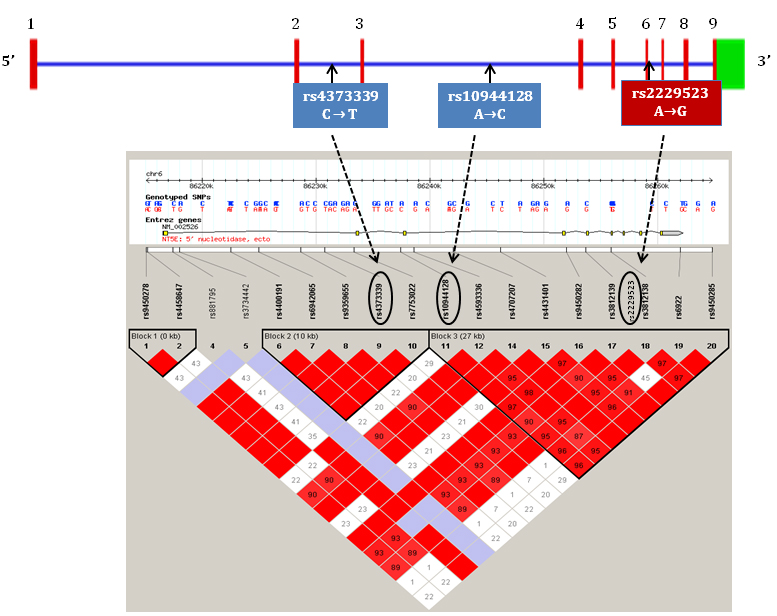
Figure 1. Schematic representation of NT5E gene with exons, introns, LD blocks and genotyped tagSNPs.

Material and Methods

Patients

Pre-dialysis CKD patients (stage 2–5) enrolled in The London Arterial Calcification, Kidney and Bone Outcomes (LACKABO) study, a single-centre prospective study aimed to assess the natural history of vascular calcification were studied [23]. Men were included if their serum creatinine was greater than or equal to 150 μmol/l and women were included if their serum creatinine was greater than or equal to130 μmol/l. All participants were 18 years or older. Patients were excluded if on renal replacement therapy. 302 patients were originally recruited into this study at baseline. However, arterial calcification scores and genetic data were available for only 229 and 279 participants, respectively, unless otherwise stated in the tables. Therefore, the primary phenotype-genotype analysis was performed on these participants, hence the number of subjects differed for each analysis.

After a mean of 49 months, participants were invited again to have follow-up scans and just over 50% of patients attended. The study complied with the Declaration of Helsinki, ethical approval was obtained from the Local Research Ethics Commitees and written informed consent provided by all study participants.

Demographic and clinical characteristics

Demographic data including age, gender, height and weight were recorded and BMI calculated at study entry (baseline). Past and present medical history, prescribed medications and cardiovascular risk factors were also noted. Majority of the patients were Caucasians (72.5%) and others included were Asians (12.3%), Black (9.5%), Chinese (1.7%) and of mixed ethnicity (4%).

Arterial calcification phenotype measurements

Coronary artery calcification (CAC) and aortic calcification (AC)

Coronary artery and aortic calcification was measured using Electron Beam Computed Tomography (EBCT). Briefly, the scanning was performed at the Royal Brompton Hospital, London using a C-150 scanner (GE-Imatron) with a 100 msec scanning time and a single slice of 3mm for the section between the carina to the level of the diaphragm. 36 to 40 slices were obtained during a single-breathhold. Patients were exposed to an overall radiation dose (0.9 msv), which is equivalent to approximately one third of the annual exposure from background radiation. CAC and AC scores were determined from the computed pixels of calcification. A pixel was defined as having a minimal density of 130 Hounsefield units (HU) and a surface area of >0.51mm². Calcification was defined as a plaque of at least 3 contiguous pixels of calcification. Calcification scores were recorded in both the aorta and in individual coronary arteries including the left circumflex, left main stem, left anterior descending, and right coronary artery. The total coronary calcification score was determined by averaging the four individual arterial scores and this value was used for subsequent analysis.

There are no agreed cut-off values for EBCT calcification score categories. We therefore, used the 5 numerical categories used by Shaw et al [24]. and adapted it by applying a descriptive term to each category (ranging from low to very high), based on category interpretations from a recent systematic review [25]: 0–10 (low); 10.1–100 (moderate); 101–400 (moderately high); 400–1000 (high); >1000 (very high).

Bone mineral density (BMD)

BMD was assessed in 238 patients from individual EBCT scans described above, which were performed to assess aortic calcification. The average of 3 lumbar vertebrae on each EBCT scan was used to calculate BMD and used in the subsequent analysis.

Blood pressure (BP) and aortic pulse wave velocity (aPWV)

All measurements were obtained in a quiet temperature-controlled room. Peripheral blood pressure and heart rate were recorded from the brachial artery of the non-dominant arm using validated oscillometric technique (HEM-705CP; Omron Corporation). aPWV, defined as the speed of pulse waves travelling along the length of an artery, was determined from sequential readings of ECG-gated carotid and femoral artery waveforms using SphygmoCor system [26]. All measurements were made in duplicate and average values were used for analysis.

Biochemical markers

Blood samples were obtained to measure vascular calcification-related biomarkers including blood lipids, glucose, serum creatinine, urea, calcium, phosphate. Estimated glomerular filtration rate (eGFR) was calculated from serum creatinine using the Modification of Diet in Renal Disease method [27].

Genetic analysis

Genomic DNA (gDNA) was isolated using standard method and stored at -80^oC for genetic analysis. Allelic discrimination was performed using AB17500 Taqman system and Taqman SNP genotyping assays (Applied Biosystems). Briefly, each assay contains two fluorescent-labelled probes corresponding to the alleles harboured by the SNP of interest. The probes carry reporter fluorescent dyes that are cleaved and released into solution during PCR by Taq polymerase when the corresponding DNA is being replicated. The colour of the released dye identifies the genotype; this is detected when the assay is analysed using the accompanying Taqman software (version 2.0.4).

For genotyping, 1ng of gDNA was mixed with 2x Taqman Universal Master Mix, No AmpErase UNG, labelled probe (FAM and VIC dye-labelled) and MQ H₂O to a total volume of 15 µL for each sample. This mixture was dispensed into a standard MicroAMP^TM Optical 96-Well Reaction Plate, and amplified using Taqman real-time PCR system. Postive and negative standards were also included on each plate. The PCR conditions consisted of a pre-PCR read at 60^oC (1min), a holding stage at 95^oC (10min), followed by 46 PCR cycles (15 secs at 95 ^oC, 1min at 60 ^oC for each cycle) and a final post-PCR read at 60^oC (1min). Allelic discrimination was carried out by detecting allele specific fluorescence and data was analysed off-line with the sequence detectionsoftware. If the genotype clusters were unambiguous, manual calling was performed or the sample was re-genotyped for that SNP. As small amounts of DNA was available in some patients, the company recommended reaction mixture concentrations were adjusted for all assays and all samples. These concentrations have been standardised and used in our previous genetic studies (>95% success rate).

Statistical analysis

Data were analysed using SPSS (version 25.0) and GraphPad Prism (version 5.0) software. All variables were checked for normal distribution and skewed variables were transformed before further analysis. Normally distributed data are presented as means ± standard deviation (SD), skewed data as median and inter-quartile range (IQR) and as geometric means, and categorical data as percentages. Oneway analysis of variance (ANOVA) was used to investigate the genotype differences in phenotype(s), and Welch’s t-tests compared average BMD and aPWV differences between the two homozygous allele carriers. And since rs2229523 SNP showed a dose dependent pattern of inheritance on BMD, SNP association was tested assuming a standard additive model using a regression analysis that adjusted for known factors that influence the calcification process (age, gender, MAP, eGFR). Paired t-tests were performed to see changes in BMD and aPWV after 49 months. A p-value of <0.05 was considered significant, in all statistical tests.

Results

Demographic, clinical and calcification-related characteristics at baseline

Demographic and baseline clinical characteristics of the LACKABO study participants are given in Table 1. The mean age was 57.8 years (age range: 19–91) and the eGFR average was 40.4 ml/min, consistent with pre-dialysis stage 3 CKD. As expected, 80% of these patients were hypertensive, 20% had diabetes and 8% had a past incident of myocardial infarction. About half of these CKD patients were also on cardiovascular drugs; hence the lipid profile and blood pressures were in the normal range (Tables 1–2).

Table 1. Clinical and demographic characteristics in 302 subjects.

BMI = body mass index; eGFR = estimated glomerular filtration rate;
CVD = cardiovascular disease; BP = blood pressure; HDL = high density lipoprotein;
LDL = low density lipoprotein.
† = median with interquartile range.

Table 2. Vascular calcification and other related measures.

BP = blood pressure; aPWV = aortic pulse wave velocity.
† = median with interquartile range.

The results for arterial calcification and other related markers are presented in Table 2. Approximately 12% of patients were in the highest score category of >1000, and median score for the population was 46.6 (IQR: 0.0–344.3). Exclusion of those with a calcification score of 0 (n = 74), resulted in a median calcification score of 169.5 (IQR: 42.9–681.8).

Genotype and allele frequencies

Two hundred and seventy nine patients had DNA available, and all samples were successfully genotyped for rs2229523 and rs4373339 SNPs, but for rs10944128 only 236 samples were genotyped due to DNA depletion. Hardy-Weinberg equilibrium was satisfied for rs2229523 and rs4373339 SNPs, but not for rs10944128 SNP. This could be due to the difficulty in calling the genotypes accurately or the assay failure for this SNP. The minor allele frequencies were similar when compared to CEU HapMap data (0.28 versus 0.30 for rs2229523, 0.17 versus 0.13 for rs4373339, and 0.45 versus 0.39 for rs10944128 respectively).

Association of NT5E SNPs with BMD and aPWV, but not with arterial calcification indices

One way ANOVA demonstrated whether patient genotypes differed for BMD and aPWV (Table 3), whilst Welch’s t-test examined differences in the phenotype between the two homozygous allele carriers (Figure 2). Only rs2229523 SNP, showed a significant association and an allele dose trend with BMD. Patients with AA genotype demonstrated significantly lower BMD values than patients with GG genotypes (93.9 versus 125.7 mg/cm³, p = 0.0182) at baseline screening (Figure 2). A similar trend was also noted in patients screened after 49 months (80.4 versus 109.4 mg/cm³, p = 0.0126). In regression models adjusted for age, gender, mean arterial pressure and eGFR, rs2229523 AA genotype was also associated with a lower BMD. As seen in Table 4, the AA genotype remained significantly and independently associated with BMD in patients screened at baseline and during follow-up. These findings held true when data were analysed excluding non-Europeans and patients on CVD drugs.

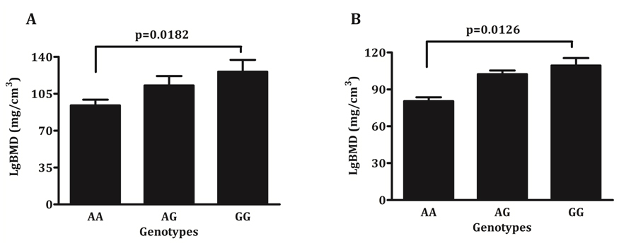
Figure 2. Average bone mineral density according to rs2229523 genotypes, A) Baseline and B) Follow-up.

Table 3. Genotype differences in BMD and aPWV at baseline and follow-up.

* Geometric means and SD
** Welch’s t-test comparing two homozygous allele carriers.

Table 4. Stepwise regression results showing an independent association of rs2229523 SNP with log transformed BMD.

Excluded variables in baseline model were: mean arterial pressure, eGFR.
Excluded variables in follow-up model were: gender, mean arterial pressure, eGFR.

Genotype differences were found with aPWV for rs2229523 SNP (Table 3); aPWV is reduced in patients carrying the rs2229523 AA genotype compared with the GG genotype. This non-significant trend was observed at both visits (baseline: 7.84 versus 8.63 m/s, p=0.350; follow-up: 7.19 versus 7.28 m/s, p=0.901).

No association was found between the SNPs and the arterial calcification indices (CAC, AC) in this CKD group.

Changes in BMD and aPWV at 49 months

Follow up data was available for just over 50% of the participants who returned for a scan. After a mean of 49 months, the vascular bone axis marker (BMD) reduced significantly (113.9 versus 103 mg/cm³;
p = 0.0002; Figure 3), whilst the aPWV reduced to a much lesser extent (8.55 versus 7.89 m/s; p = 0.057, data not shown).

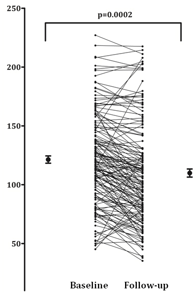
Figure 3. Average bone mineral density values at baseline and follow up.

Associations between age and calcification phenotypes

As expected, age associated significantly with BMD, PWV, CAC and AC (r = –0.46, r = 0.49, 0.60, 0.51; p = 0.001 respectively, data not shown), and when this relationship was explored further by examining just CAC in men and women according to decades of age, the average CAC score increased with each decade in both men and women (Table 5); the lowest mean values were observed in the younger patients and highest values in older patients.

Table 5. Coronary artery calcification score in CKD patients by age and gender.

SEM = standard error of mean.

BMD also associated inversely with AC (r = –0.30, p = 0.001, data not shown) and aPWV (r = –0.16, p = 0.032, data not shown), which suggests that low BMD and increasing arterial calcification have common features [28]. The positive correlation between calcification scores and stiffness (aortic: 0.40, p = 0.001; coronary artery: 0.22, p = 0.015, data not shown), demonstrates the associated changes in the vessel wall of CKD patients [29].

Discussion

This study sought to determine the influence of common SNPs in the NT5E gene on calcification phenotypes (BMD, aPWV) in pre-dialysis CKD patients. For the first time, we identified a significant independent association between a single NT5E gene polymorphism (rs2229523 SNP) and BMD, a marker of the vascular-bone axis. Independent of risk factors like age, gender, mean arterial pressure and eGFR, we found that rs2229523 AA genotype associated with lower BMD. This relationship was found in patients screened both at baseline and after 49 months of follow up. The rs2229523 AA genotype also showed reduced aortic stiffness (aPWV). However, no independent SNP associations were observed with aPWV or with coronary artery or aortic calcification (CAC, AC).

Significant association between rs2229523 SNP and BMD

The finding that an NT5E rs2229523 SNP is associated with BMD suggests a role for CD73 in bone formation. This is supported by the finding of osteopenia, reduced osteoblastic markers and impaired osteroblastic differentiation in CD73 knockout mice [30]. In the same study, induced overexpression of CD73 was associated with increased osteoblastic differentiation, and increased expression of osteocalcin and bone sialoprotein, the effects of which were reversed by an A_2B receptor antagonist [30]. These findings suggest that the effects of CD73 on bone metabolism are mediated by CD73-derived adenosine signalling. The role of CD73 in bone metabolism is further supported by another study where CD73 expression is regulated by the Wnt-b-catenin signalling pathway, a known critical pathway in both bone metabolism and osteogenic vascular calcification [31]. In addition, the inducible HIF-1 alpha transcription factor, which regulates many factors involved in bone regeneration and development, also regulates CD73 expression [32].

The regression analysis findings suggest that rs2229523 AA genotype predicts a lower BMD after adjustments of confounding factors like age, gender, mean arterial pressure and eGFR. The exact mechanisms behind the the lower BMD and reduced aPWV observed in patients with AA genotype are currently unclear and outside the scope of this study, but merits further investigation. The SNP in question is a non-synonymous coding SNP which results in a change in amino-acid from threonine to alanine at position 376. It is believed that this results in an alternative shorter isoform of the protein. The clinical implication of this isoform change is not known, but this is the first study linking this SNP to BMD. As rs2229523 is a tagSNP, the observed relationship may relate to this amino-acid change or may, alternatively, relate to another SNP within the same LD block.

None of the SNPs in this study, associated with BMD or bone mineral content in published genome wide association studies (GWAS) [33,34], and this could be explained by the populations or phenotypes studied or the genechips used. But the present finding of an association between BMD and rs2229523 SNP, and its role in the regulation of vascular calcification is not surprising given the known reciprocal and parallel relationship between arterial and skeletal mineralisation. A significant inverse assocation between vascular calcification and BMD has been demonstrated in non-CKD populations [35] as well as in dialysis [2] and pre-dialysis CKD populations [29], a finding replicated in our study. This relationship appears to be particularly strong in CKD, which provides an ideal milieu for both arterial calcification and osteopenia due to synergism between hyperphosphataemia, hyperparathyroidism, and the treatments associated with CKD [29,36]. Pre-clinical studies showed that inflammatory markers such as lipids and cytokines appear to accelerate vascular calcification while they promote bone loss [38]. Similarly, osteogenic agents, like PTH and BMP-7, promote skeletal mineralisation but suppress this process in arteries [36]. The mechanism linking arterial calcification to bone loss is unknown and the temporal nature of events has not been established. One theory is that both share a common aetiology and use common factors [38]. CD73 provides a link between the two conditions; its osteogenic role in bone in parallel with its anti-inflammatory role in the vasculature would result in bone loss and calcification in the event of deficiency, consistent with the reciprocal relationship observed between the two conditions.

Significant associations found between arterial calcification phenotypes, but not between calcification phenotypes and NT5E SNPs

We replicated previous positive associatons between age, arterial calcification (aortic and coronary artery) and arterial stiffness (aPWV) [29, 37, 38]. However, we did not find these phenotypes to associate with any of the NT5E SNPs. There are several possible explanations for the lack of associations between the SNPs and arterial calcification. First, the inability to measure medial calcification independent of intimal calcification may have prevented detection of an association. Histopathological evidence from specimens derived from arterial calcification due to deficiency of CD73 (ACDC) patients suggest, that the calcification process resulting from CD73 deficiency is confined to the arterial media [20]; therefore, medial calcification is the relevant phenotype. As current instruments do not have the capability of distinguishing between medial and intimal calcification [39], the measured phenotype in this study was actually an aggregate of both intimal and medial calcification, diluting the relevant phenotype.

Second, the lack of an assocation might be due to measurement of central artery rather than peripheral artery calcification. It is important to note that the ACDC phentotype is characterised by heavy calcification specifically in the large lower limb peripheral arteries, with relative sparing of the coronary and aortic arteries [20,13]. Therefore, a CD73-related protein family member, such as CD39, or its related isoforms, may compensate for CD73 deficiency in other vascular beds [40]. Given this, it is not surprising that NT5E SNPs were not associated with coronary or aortic calcfication in this study.

Third, it is possible that the relationship between NT5E mutations and calcification observed in ACDC [12] is non-causal. The proposed mechanism linking CD73 deficiency to arterial calcification is based upon in vitro experiments in skin fibroblasts [12], which may differ signficantly from vascular endothelial cells. Furthermore, the vascular calcification phenotype has not been recapitulated in in vivo mice studies, where CD73 deletion has been found to be associated with multi-organ fulminant vascular leakage rather than calcification [41].

Fourth, it may be that NT5E genetic variation does cause calcification but it does not do so by affecting the essential pyrophosphate pathway, instead it affects non-essential pathways. For example, the calcification phenotype produced by NT5E mutations is more likely to be explained by the anti-inflammatory role of CD73 rather than its indirect effects on pyrophosphate hydrolysis [42]. A polymorphism in an anti-inflammatory pathway is less likely to be of clinical significance due to the upregulation of alternative anti-inflammatory pathways in CKD.

Lastly, 27% of patients had an arterial calcification score of 0, which resulted in reduced power, and the SNPs investigated do not represent the whole gene, so it is possible that relevant variations reside in the other unexplored regions. Therefore, the relationship between NT5E genetic variation and arterial calcificaiton merits further investigation and replication in other independent CKD population.

Conclusion

For the first time, we have shown that rs2229523, a non-synonymous coding SNP resulting in an amino-acid change (threonine to alanine), and AA genotype is associated with lower BMD in patients with CKD seen before and after 49 months . Further work is necessary to evaluate the identified associations in other CKD cohorts. Functional studies are also required to elucidate the biological mechanisms underlying the observed relationship between NT5E rs2229523 SNP and BMD. The role of adenosine, adenosine regulators and adenosine receptor agonists as potential therapeutic agents in relation to vascular calcification and osteopenia also warrants extensive further exploration. Overall, this study offers new insights into the bone-vascular axis in chronic kidney disease, identifying a novel role for CD73 of potential clinical importance.

Acknowledgements We thank all the individuals who participated in the LACKABO study. The LACKABO study participants were recruited by a grant from the Kidney Research (Grant No. VC1/2002), and the genotyping costs were supported by the Addenbrooke’s Charitable Trust (Ref No. 23/08(B) (F). We also thank Dr Michael Rubens for performing scans, Dr Sharon Barrett and Dr Melanie Chan with pulse wave analysis measurements.

Conflict of interest The authors declare no conflict of interest.

References

1. Blacher J, Guerin AP, Pannier B, Marchais SJ, London GM. (2001) Arterial Calcifications, Arterial Stiffness, and Cardiovascular Risk in End-Stage Renal Disease. Hypertension. 38(4): 938–42.
2. Aoki A, Kojima F, Uchida K, Tanaka Y, Nitta K. (2009) Associations between vascular calcification, arterial stiffness and bone mineral density in chronic hemodialysis patients. Geriatrics & Gerontology International. 9(3): 246–52.
3. Blacher J, Guerin AP, Pannier B, Marchais SJ, Safar ME, London GM. (1999) Impact of aortic stiffness on survival in end-stage renal disease. Circulation. 99(18): 2434–9.
4. Shoji T, Emoto M, Shinohara K, Kakiya R, Tsujimoto Y, Kishimoto H, et al. (2001) Diabetes mellitus, aortic stiffness, and cardiovascular mortality in end-stage renal disease. Journal of American Society of Nephrology. 12(10): 2117–24.
5. Goodman WG, London G, Amann K, Block Ga, Giachelli C, Hruska Ka, et al. (2004) Vascular calcification in chronic kidney disease. American Journal of Kidney Diseases. 43(3): 572–9.
6. Román-García P, Rodríguez-García M, Cabezas-Rodríguez I, López-Ongil S, Díaz-López B, Cannata-Andía JB. (2011) Vascular calcification in patients with chronic kidney disease: types, clinical impact and pathogenesis. Medical Principles and Practice. 20(3): 203–12.
7. Schinke T, Karsenty G. (2000) Vascular calcification–a passive process in need of inhibitors. Nephrology Dialysis Transplantation. 15(9): 1272–4.
8. Schinke T, McKee MD, Kiviranta R, Karsenty G. (1998) Molecular determinants of arterial calcification. Annals of Medicine. 30(6): 538–41.
9. Schoppet M, Shanahan CM. (2008) Role for alkaline phosphatase as an inducer of vascular calcification in renal failure? Kidney International. 73(9): 989–91.
10. Meyer JL. (1984) Can biological calcification occur in the presence of pyrophosphate? Archives of Biochemistry and Biophysics. 231(1): 1–8.
11. Rutsch F, Vaingankar S, Johnson K, Goldfine I, Maddux B, Schauerte P, et al. (2001) PC-1 nucleoside triphosphate pyrophosphohydrolase deficiency in idiopathic infantile arterial calcification. American Journal of Pathology. 158(2): 543–54.
12. Eller P, Hochegger K, Feuchtner GM, Zitt E, Tancevski I, Ritsch A, et al. (2008) Impact of ENPP1 genotype on arterial calcification in patients with end-stage renal failure. Nephrology Dialysis Transplantation. 23(1): 321–7.
13. St Hilaire C, Ziegler SG, Markello TC, Brusco A, Groden C, Gill F, et al. (2011) NT5E mutations and arterial calcifications. The New England Journal of Medicine. 364(5): 432–42.
14. Sharp J. (1954) Heredo-familial vascular and articular calcification. Annals of the Rheumatic Diseases. 13(1): 15–27.
15. Mori H, Yamaguchi K, Fukushima H, Oribe Y, Kato N, Wakamatsu T, et al. (1992) Extensive arterial calcification of unknown etiology in a 29-year-old male. Heart Vessels. 7(4): 211–4.
16. Zhang Z, He JW, Fu WZ, Zhang CQ, Zhang ZL. (2015) Calcification of joints and arteries: second report with novel NT5E mutations and expansion of the phenotype. Journal of Human Genetics. 60(10): 561–4.
17. Yoshioka K, Kuroda S, Takahashi K, Sasano T, Furukawa T, Matsumura A. (2017) Calcification of joints and arteries with novel NT5E mutations with involvement of upper extremity arteries. Vascular Medicine. 22(6): 541–3.
18. O’Neill WC, Sigrist MK, McIntyre CW. (2010) Plasma pyrophosphate and vascular calcification in chronic kidney disease. Nephrology Dialysis Transplantation. 25(1): 187–91.
19. Colgan SP, Eltzschig HK, Eckle T, Thompson LF. (2006) Physiological roles for ecto-5’-nucleotidase (CD73). Purinergic Signal. 2(2): 351–60.
20. Markello TC, Pak LK, St C, Dorward H, Ziegler SG, Chen MY, et al. (2011) Vascular pathology of medial arterial calcifications in NT5E deficiency: implications for the role of adenosine in pseudoxanthoma elasticum. Molecular Genetics & Metabolism. 103(1): 44–50.
21. Hasegawa T, Bouis D, Liao H, Visovatti SH, Pinsky DJ. (2008) Ecto-5’ nucleotidase (CD73)-mediated adenosine generation and signaling in murine cardiac allograft vasculopathy. Circulation Research. 103(12): 1410–21.
22. Rutsch F, Nitschke Y, Terkeltaub R. (2011) Genetics in arterial calcification: pieces of a puzzle and cogs in a wheel. Circulation Research. 109(5): 578–92.
23. Caplin B, Nitsch D, Gill H, Hoefield R, Blackwell S, MacKenzie D, et al. (2010) Circulating methylarginine levels and the decline in renal function in patients with chronic kidney disease are modulated by DDAH1 polymorphisms. Kidney International. 77(5): 459–67.
24. Shaw LJ, Raggi P, Schisterman E, Berman DS, Callister TQ. (2003) Prognostic value of cardiac risk factors and coronary artery calcium screening for all-cause mortality. Radiology. 228(3): 826–33.
25. Dendukuri N, Chiu K, Brophy JM. (2007) Validity of electron beam computed tomography for coronary artery disease: asystematic review and meta-analysis. BMC Medicine. 5: 35.
26. Wilkinson IB, Fuchs SA, Jansen IM, Spratt JC, Murray GD, Cockcroft JR, et al. (1998) Reproducibility of pulse wave velocity and augmentation index measured by pulse wave analysis. Journal of Hypertension. 16(12 Pt 2): 2079–84.
27. Hallan S, Asberg A, Lindberg M, Johnsen H. (2004) Validation of the Modification of Diet in Renal Disease formula for estimating GFR with special emphasis on calibration of the serum creatinine assay. American Journal of Kidney Disease. 44(1): 84–93.
28. Kooman JP, Kotanko P, Schols AM, Shiels PG, Stenvinkel P. (2014) Chronic kidney disease and premature ageing. Nature Reviews Nephrology. 10(12): 732–42.
29. Toussaint ND, Lau KK, Strauss BJ, Polkinghorne KR, Kerr PG. (2008) Associations between vascular calcification, arterial stiffness and bone mineral density in chronic kidney disease. Nephrology Dialysis Transplantation. 23(2): 586–93.
30. Takedachi M, Oohara H, Smith BJ, Iyama M, Kobashi M, Maeda K, et al. (2012) CD73-generated adenosine promotes osteoblast differentiation. Journal of Cellular Physiology. 227(6): 2622–31.
31. Spychala J, Kitajewski J. (2004) Wnt and beta-catenin signaling target the expression of ecto-5’-nucleotidase and increase extracellular adenosine generation. Experimental Cell Research. 296(2): 99–108.
32. Synnestvedt K, Furuta GT, Comerford KM, Louis N, Karhausen J, Eltzschig HK, et al. (2002) Ecto-5’-nucleotidase (CD73) regulation by hypoxia-inducible factor-1 mediates permeability changes in intestinal epithelia. Journal of Clinical Investigation. 110(7): 993–1002.
33. Rivadeneira F, Styrkársdottir U, Estrada K, Halldórsson BV, Hsu YH, Richards JB, et al. (2009) Twenty bone-mineral-density loci identified by large-scale meta-analysis of genome-wide association studies. Nature Genetics. 41(11): 1199–206.
34. Styrkarsdottir U, Halldorsson BV, Gretarsdottir S, Gudbjartsson DF, Walters GB, Ingvarsson T, et al. (2009) New sequence variants associated with bone mineral density. Nature Genetics. 41(1): 15–7.
35. Lin T, Liu JC, Chang LY, Shen CW. (2011) Association between coronary artery calcification using low-dose MDCT coronary angiography and bone mineral density in middle-aged men and women. Osteoporosis International. 22(2): 627–34.
36. Demer LL, Tintut Y. (2008) Vascular calcification: pathobiology of a multifaceted disease. Circulation. 117(22): 2938–48.
37. Raggi P, Bellasi A, Ferramosca E, Islam T, Muntner P, Block GA. (2007) Association of pulse wave velocity with vascular and valvular calcification in hemodialysis patients. Kidney International. 71(8): 802–7.
38. Temmar M, Liabeuf S, Renard C, Czernichow S, Esper NE, Shahapuni I, et al. (2010) Pulse wave velocity and vascular calcification at different stages of chronic kidney disease. Journal of Hypertension. 28(1): 163–9.
39. Goodman WG, London G. (2004) Vascular Calcification in Chronic Kidney Disease. American Journal of Kidney Diseases. 43(3): 572–9.
40. Rutsch F, Nitschke Y, Terkeltaub R. (2011) Genetics in arterial calcification: Pieces of a puzzle and cogs in a wheel. Circulation Research. 109(5): 578–92.
41. Thompson LF, Eltzschig HK, Ibla JC, Van De Wiele CJ, Resta R, Morote-Garcia JC, et al. (2004) Crucial role for ecto-5’-nucleotidase (CD73) in vascular leakage during hypoxia. The Journal of Experimental Medicine. 200(11): 1395–405.
42. Schrader J. (2011) NT5E mutations and arterial calcifications. The New England Journal of Medicine. 364(16): 1578–9.

DOI: 10.31038/JCRM.2018124

Abstract

Our case focuses on a patient with a rare mutation, 9pter-9p22.2 interstitial deletion, associated with unique presentation and specific cardiac abnormalities which have not previously been associated with this condition. The subject was a term male infant born with an omphalocele which had been diagnosed prenatally. Upon delivery he was noted to have craniofacial and limb abnormalities, and found to be persistently hypoglycemic, requiring a significantly elevated glucose infusion rate. On echocardiogram an aortic coarctation was identified. He underwent cardiac repair, but ultimately developed severe pulmonary hypertension complicated by multiple episodes of cardiopulmonary arrest. To our knowledge there are only 26 previously identified patients with similar copy number variants on this region reprinted in the literature or identified in the Decipher database. This case report is not only able to help build knowledge which can be used to predict phenotypes, but it can also shed light on some of the more devastating characteristics possible with this condition. While this subject did have two of the most common symptoms involved, craniofacial and musculoskeletal, he also had cardiovascular abnormalities, which had only been identified in one other patient with 9pter-9p22.2 interstitial deletion. It was also a goal of this report to identify similarities and differences between 9pter-9p22.2 interstitial deletion with the much more well-known disease, 9p minus syndrome. Of patients with 9p minus, craniofacial and musculoskeletal abnormalities are very common. Patients also frequently have visceral defects, intellectual disabilities, hypoglycemia, genital defects, and a small incidence of cardiovascular defects. More subjects are needed for further evaluation, but it appears that 9pter-9p22.2 interstitial deletion may be much more similar to the larger 9p minus syndrome than previously appreciated.

Introduction/Background

Current advancements in pediatric critical care as well as the evolution of human genomic investigations have revealed a wide range of clinical pathologies warranting further classification and, in-turn, clinical correlations by providers. The DECIPHER database has focused on cataloguing specific mutations with correlated phenotypes to better characterize genetic abnormalities [1].

9p deletion syndrome is a pathologic genetic copy number variant initially identified in 1973 by Alfi and colleagues [2]. Since this time, more than 100 cases of 9p minus have been reported worldwide. The syndrome represents a heterogeneous condition, characterized upon initial presentation with craniofacial abnormalities (including trigonocephaly, midface hypoplasia, upslanting palpebral fissures, anteverted nostrils, depressed nasal bridge, long philtrum, and hypertelorism), short neck, increased inter-nipple distance, positional limb defects, nonketotic hypoglycemia, external genitalia anomalies, and cardiac abnormalities [3]. Follow up and longitudinal assessments demonstrate neurocognitive difficulties including low IQ (mean of 49), global developmental delays, hypotonia, and behavioral problems [4]. Visceral abnormalities including inguinal or umbilical hernias and omphaloceles have also been reported [5,6]. Swinkels et al. previously observed approximately 15% of patients with 9p- syndrome had an omphalocele [7].

More specifically, 9pter-9p22.2 interstitial deletion, is a micro-deletion syndrome which has demonstrated an emerging clinical significance and has currently been diagnosed in 26 patients across the globe. As shown in Table 1, these patients share many phenotypic similarities to 9pminus, but 9pter-9p22.2 interstitial deletion is subtyped with an even stronger association with craniofacial deformities and developmental delays [8].

With the apparent rise in the frequency of 9pminus diagnosis and concomitant presentations of the 9pter-9p22.2 interstitial deletion subtype, our report serves to catalogue and summarize the available data to provide initial diagnosing providers and follow up clinicians with a more robust clinical picture to best manage these complex patients.

Table 1. Phenotypic abnormalities in known patients with 9pter-9p22.2 interstitial deletion [8].

Clinical Report

The subject of concern was a term male singleton born to a 25 year old G3P1 mother with insignificant past medical history. The pregnancy management involved a multi-disciplinary approach including maternal fetal medicine, neonatology, pediatric cardiology, and genetics due to concern for omphalocele with hepatic effect appreciated on prenatal anatomy ultrasound.

The child was delivered via scheduled cesarean section and received routine newborn resuscitation from the intensive care team with the use of a bowel bag. The initial transition period was complicated by hypoglycemia requiring a glucose intravenous infusion bolus in addition to an escalation of the glucose infusion rate to a maximum 9.9 mg/kg/min at 24 hours of life.

The patient’s remarkable findings on physical exam consisted of: frontal bossing with prominent metopic ridge, up-slanting palpebral fissures, posteriorly rotated ears; heart sounds auscultated with continuous machine-like murmur; 3 cm omphalocele; wide-spaced nipples; sandal gap deformity, talipes equinovares of the left foot.

Given the patient’s constellation of clinical signs and symptoms, the neonatal team proceeded down the diagnostic pathway for Beckwith Wiedemann syndrome by obtaining an echocardiogram. The study revealed biventricular hypertrophy with normal function, a hypoplastic transverse arch with coarctation, and a PFO with left to right shunting. Following intubation in preparation for transfer, the patient was started on Prostaglandin 0.05mcg/kg/min. Prior to transfer, and due to the presumptive clinical diagnosis of Beckwith Wiedemann, blood was obtained for genetic analysis. This investigation later revealed the etiology of the child’s defects was 9pter-9p22.2 interstitial deletion.

After transfer to a higher level of care, the child underwent aortic arch repair. Preoperative echocardiogram demonstrated moderate to severe hypoplasia of the transverse and distal arch, multiple ventricular septal defects (perimembranous and muscular) with occasional bi-directional shunting, a stable atrial septal defect, as well as a bicuspid aortic valve. He ultimately required multiple surgeries including the previously stated aortic arch repair, hemidiaphragm plication, tracheostomy, gastrostomy-tube with Nissen fundoplication, and omphalocele repair. He spent several weeks in intensive care units during which multiple desaturation and code events occurred. Ultimately, at 5 months of life, palliative measures were put in place and shortly after the child died.

Discussion

The purpose of this report was to present the current knowledge known on 9pter-9p22.2 interstitial deletion, expand the available literature concerning the more well recognized 9p minus syndrome, and compare 9p minus syndrome to 9pter-9p22.2 interstitial deletion. This will ideally enable providers to better identify this subtype, as well as formulate appropriate treatment, surveillance, and prognostic plans.

The available cases of 9pter-9p22.2 interstitial deletion revealed craniofacial abnormalities (38.5%), developmental delays (38.5%) and musculoskeletal abnormalities (23%) as the most common features typically identified. While our subject exhibited craniofacial and musculoskeletal abnormalities, he also demonstrated a less well recognized condition: congenital cardiac abnormalities. Prior to this report only one patient had been identified with cardiac dysfunction. While it is unclear specifically what cardiac abnormalities the previous patient had, our patient had significant cardiovascular compromise, including aortic coarctation, aortic hypoplasia, an atrial septal defect, ventricular septal defects and a bicuspid aortic valve. Due to such a small sample size, each additional patient with a specific feature, such as cardiac abnormalities has the potential to change the current associated risk related to that feature. Ultimately, subjects with the more common craniofacial and musculoskeletal abnormalities may warrant baseline echocardiograms and chest radiographs to evaluate for congenital cardiac defects. This may facilitate early recognition of deadly, congenital defects and hasten transfer, management and therapy at the appropriate facility.

Conclusion

Ideally, this report will aid clinicians in identifying and managing patients with 9pter-9p22.2 interstitial deletion. It is a significant copy number variant which, while sometimes fairly benign, has the potential to be devastating, and potentially fatal. Patients with confirmed or suspected 9pter-9p22.2 interstitial deletion would likely benefit from cardiovascular screening as well as potential transfer to a pediatric heart center.

Conflicts of Interest and Source of Funding:  Salary support was provided for Drs. Koslow, Reeves, Anchan, and Rohena by the United States Department of Defense. The authors have no conflicts of interest.

Disclaimer: This work was prepared as part of the official duties of Drs. Koslow, Reeves, Anchan, and Rohena who are employed by the United States Army and Air Force. The views expressed in this article are those of the authors and do not reflect the official policy or position of the United States Army, Air Force, Department of Defense, or the United States Government. Title 17 U.S.C. 105 provides that “Copyright protection under this title is not available for any work of the United States Government.” Title 17 U.S.C. 101 defines a United States Government work as a work prepared by a military service member or employee of the United States Government as part of that person’s official duties.

This study makes use of data generated by the DECIPHER community. A full list of centres who contributed to the generation of the data is available from hhttp: //decipher.sanger.ac.uk and via email from decipher@sanger.ac.uk. Funding for the project was provided by Wellcome.

Authors contributions:

Elizabeth Koslow conceptualized the study, interpreted the data analysis, drafted the manuscript, and approved the final manuscript.

Patrick Reeves conceptualized the study, interpreted the data analysis, drafted the manuscript, and approved the final manuscript.

Joshua Anchan contributed to study design, developed the data analysis plan, interpreted the data, and revised the manuscript.

Luis Rohena contributed to study design, interpreted the data, and revised the manuscript.

All authors approved the final version of the manuscript.

References

1. Antonarakis, S. E. (2013). Human Gene Mutation in Inherited Disease: Molecular Mechanisms and Clinical Consequences. In D. Rimoin (Ed.), Emery and Rimoin’s Essential Medical Genetics. Elsevier/AP.
2. Alfi OS. (1973) Delation of the short arm of chromosome# 9 (46, 9P-): A new deletion syndrome. Ann Genet. 16: 17–22.
3. Boby, J., Karande, S., Lahiri, K., Jain, M., & Kanade, S. (1994). 9p-Syndrome. Journal of Postgraduate Medicine. 40(1), 40–1.
4. Jones, K., Jones, M., & Del Campo, M. (2013). Deletion 9P Syndrome (9P Monosome, 9P- Syndrome). In Smith’s Recognizable Patterns of Human Malformation. Elsevier Health Sciences .
5. Spazzapan, P., Arnaud, E., Baujat, G., Nizon, M., Malan, V., Brunelle, F., & Di Rocco , F. (2016). Clinical and neuroradiological features of the 9p deletion syndrome. Child’s Nervous System, 32(2), 327–335. [Crossref]
6. Hou, Q.-F., Wu, D., Chu, Y., & Liao, S.-X. (2016). Clinical findings and molecular cytogenetic study of de novo pure chromosome 9p deletion: Pre- and postnatal diagnosis. Taiwanese Journal of Obstetrics and Gynecology, 55(6), 867–870. [Crossref]
7. Swinkels, M., Simons, A., Smeets, D., Vissers, L., Veltman, J., Pfundt, R., . . . van Ravenswaaii-Arts, C. (2008). Clinical and cytogenetic characterization of 13 Dutch patients with deletion 9p syndrome: Delineation of the critical region for a consensus phenotype. America Journal of Medical Genetics A, 146A(11), 1430–8. [Crossref]
8. Firth, H., Richards, S., Bevan , A., Clayton, S., Corphas, M., Rajan, D., . . . Carter, N. (2009). DECIPHER: database of chromosomal imbalance and phenotype in humans using ensemble resources. The American Journal of Human Genetics , 84(4), 524–33. [Crossref]

DOI: 10.31038/JCRM.2018123

Abstract

Aim: To review the clinical features and identify mortality risk factors of patients admitted to hospital for acute mushroom poisoning (AMP) .

Methods: We retrospectively analyzed a database of 315 patients who underwent acute mushroom poisoning between September 2003 and December 2017 at our hospital. The patients were divided into the survival group (n = 272) and death group (n = 43) based on the prognosis. Multivariate logistic regression was used to evaluate the risk factors associated with death.

Results: Overall, 315 cases were enrolled into the statistical analysis. The average age of them was 40.66 ± 20.86 years and there were 193 (61.27%) male. Patients with latency of 6–24 hours had a higher rate of composition (54.60%) and mortality (11.75%) . Liver was the most commonly involved organ (152/523, 29.06%) and patients with liver damage had the highest mortality (40/315,12.70%) . There was significant relationship between the number of organs involvement and mortality rate. Three or more organs damage could obviously increase mortality rate (P﹤0.05) . Compared with survival group, patients in death group had higher levels of alanine aminotransferase (ALT) , total bilirubin direct (TBIL) , direct bilirubin (DBIL) , prothrombin time (PT) , activated partial thrombin time (APTT) , creatine kinase MB (CK-MB) , myoglobin (Mb) , lactate dehydrogenase (LDH) and lower levels of albumin (ALB) and sodium (Na⁺) (P < 0.05) . ALT ≥ 200U/L, PT ≥ 20s and ALB≤30g/L were identified as independent risk factors of the death in AMP (P < 0.05) .

Conclusion: We found that the number of organs involvement, ALT ≥ 200U/L, PT ≥ 20s and ALB≤30g/L were significantly associated with mortality. Clinicians should be aware the dynamic changes in the above factors so that they can be detected early and treated as soon as possible.

Key words

acute mushroom poisoning; survival group; death group; clinical features; risk factors; multiple organ dysfunction syndrome; retrospective analysis

Introduction

Poisonous mushroom has many types, colors, sizes and morphologies. It is difficult to visually distinguish it from edible mushrooms. Therefore, AMP is a common phenomenon. Some poisonous mushrooms are rich in toxins, which are heat stable and not inactivated by cooking .The chemical structure of toxins is similar to the herbicides diquat and paraquat, they can lead to nausea, vomiting, abdominal pain, diarrhea and it can even make the disease progress rapidly and cause multiple organ dysfunction syndrome (MODS) to death ^[1,^2]. Amanita poisoning has long been a worldwide problem, because it accounts for about 90% of fatality^[3]. The lethal dose of α-amanitin is very low, only 0.1mg / kg, and some mushroom can contain up to 15 mg. That’s one of the reasons why the mortality of α-amanitin is high and it’s known as the most poisonous toxins ^[4,^5]. It had been reported that there were 50 to 100 deaths in Western European countries each year, and it was relatively rare in the United States, but there were also approximately 100 deaths in five years ^[6,7]. In China, the mortality of AMP is still high even as high as 21.2% and there are no special antidotes ^[8,9]. Although the disease has a high mortality rate, at present, most articles on AMP are case reports or series, and limited data exist on the clinical characteristics and possible mortality risk factors of patients admitted to hospital for AMP. To better identify the disease clinical features that are related to the fatal outcome of AMP patients admitted to hospital , we collected clinical data of 315 AMP patients admitted to our hospital from September 2003 to December 2017 and analyzed the clinical features and risk factors of the death, based on data from the initial admission.

Materials and Methods

Participant enrollment and inclusion/exclusion criteria

The patients who were diagnosed as AMP in our hospital between September 2003 and December 2017 were enrolled in the retrospective study. All these patients were included in the study according to the following inclusion: (1) . They had a clear history of eating wild poisonous mushrooms and duration did not exceed three days. (2). Co-fed persons had different symptoms of poisoning, while others had not. (3) . They all had relevant laboratory abnormalities. (4) .Clinical datas were complete and successfully received follow-up for at least six months. The patients with history of related diseases including drugs of abuse, viral hepatitis, glomerulonephritis or other which could lead to liver, kidney and other organs damage were excluded from this study. This study strictly followed the ethical principles of human medical research in the Declaration of Helsinki and was approved by the hospital ethics committee and obtained the informed consent of all patients or their relatives.

Diagnostic criterias for organs involvement

The diagnostic criterias for organs involvement were as follows: (1). Elevated alanine aminotransferase ( ≥ 200 U/L) six-fold greater than the upper limit of normal concentration (5~35 U/L) , and/or the presence of total bilirubindirect ( ≥ 35umol/L) (normal range:0~27 umol/L), both of them were defined as liver damage. (2) Increased prothrombin time ( ≥ 20s) (normal range:0~14 s) and/or activated partial thrombin time ( ≥ 40s) (normal range:20~40 s) was considered to be coagulation abnormalities. (3). Elevated creatine kinase MB ( ≥ 5ug/ml) (normal range: 0.01–4.94 ng/ml) was defined as heart involvement. (4) . Increased creatinine ( ≥ 160umol/L) double than the normal concentration (normal range:45–84 umol/L) was considered to be kidney involvement. (5). The presence of relevant symptoms and/or signs (delirium, coma, twitch and irritability) was defined as damage to nervous system. (6). The appearance of abdominal signs and increased serum amelase ( ≥ 300 U/L) three-fold greater than the upper limit of normal concentration (28–100 U/L) , and/or videography showed pancreatitis, both of them were defined as pancreas damage.

Collection of clinical information

The data we collected including gender, age, duration of hospitalization, latency period, laboratory indicators (including blood routine indexes, liver function indexes, renal function indexes, coagulation function indexes, myocardial injury markers, electrolytes indexes) and prognosis.

Statistical analysis

All statistical analyses were performed using SPSS version 22.0 for Windows (SPSS Corp, Chicago, IL, USA) . Kolmogorov-Smirnov test was used to test the normality of measurement data. Normal distribution data were expressed as the mean ± standard deviation (SD) . Inter-group comparisons of continuous variables were performed by a 2-sample t-test or t’ test when the variance was uneven. While non-normal distribution of measurement data were described using median and interquartile range (IQR) values and rank sum test was used to compare the difference between the two groups. Frequencies and percentage were used to indicate categorical variables, and inter-group comparisons were performed by Chi-square test. To identify independent factors associated with death, explanatory items were selected using univariate analysis, followed by multivariate logistic regression. We considered p values less than 0.05 as statistically significant.

Result

1. Baseline clinical features of all patients with acute mushroom poisoning

During the study period, a total number of 315 patients were enrolled, including 272 (86.35%) survival cases and 43 (13.65%) death cases. Among all the patients, 193 (61.27%) were male. The mean age was 40.66 ± 20.86 (range, 1- 92) years. Table I shows the clinical baseline datas of all patients. The mean value of first recorded laboratory indexes were as follows: ALT 111.50 (26.1, 1087.40) U/L, TBIL 19.70 (11.70, 38.70) umol/L, ALB 44.90 ± 7.39 g/L, PT 14.20 (12.70,19.40) seconds, APTT 35.00 (30.20,45.00) seconds, CK-MB 1.54 (0.52,3.71) ng/m, LDH 340.20 (211.40,875.80) U/L and Na⁺ 136.31 ± 5.93 mmol/L.

Poisonous mushroom’ colors are varied. For the specific shapes of them, such as wearing “hat”, waist “skirt”, wearing “shoes”, patients could not describe clearly. The intake amount was not equal, ranging from 20–500g. Regional distribution was significantly different, mostly in Sichuan, Yunnan and Guizhou province. Most patients were collective disease, while a small number of them was single.

2. Multiple organ involvement of all the patients

Liver (152 / 523, 29.06%) was the most affected organs, followed by heart (134 / 523, 25.62%) and coagulation system (107 / 523, 20.46%) (Figure. 1A) . The patients with liver damage had the highest mortality (40 / 315, 12.70%) , then followed by coagulation disorders (35 / 315, 11.11% ) and heart damage (34/315, 10.79%) , respectively (Figure. 1B) . In addition, the more affected organs or systems, the higher mortality rate (0.00%, 5.36%, 7.69%, 21.95%,47.37%, 53.85%). The mortality of patients with four organs damage was higher than those who had three organs damage (47.37% vs. 21.95%; P < 0.05), and the latter is higher than that of patients with two organs damage (21.95% vs. 7.69%; P < 0.05) (Figure.1C) .

3. Comparisons of clinical factors and outcomes in acute mushroom poisoning

Late onset (latent period was 6–24 hours) (86.05% vs. 49.63% ) was more common in death group and a total of 37 (11.75%) patients became dead. According to data analysis, patients in death group had higher levels of ALT (P < 0.001) , TBIL (P = 0.002) , DBIL (P < 0.001), PT (P < 0.001) , APTT (P < 0.001) , CK-MB (P < 0.001) , Mb (P < 0.001) , LDH (P < 0.001) and lower levels of ALB (P = 0.001) and Na⁺ (P < 0.001) . Table I summarizes the patients’clinical data and outcomes of AMP.

4. Risk assessment of clinical features associated with the death of acute mushroom poisoning patients

Univariate logistic regression indicated that whether or not to adjust related confounding factors (age, gender and latency) ,WBC ≥ 12×10⁹/L,ALT ≥ 200 U/L, TBIL ≥ 35umol/l, DBIL ≥ 20umol/l, ALB≤30g/L, PT ≥ 20s, APTT ≥ 40 s , CK-MB ≥ 5 μg/L, MB ≥ 140 μg/L, LDH ≥ 500 U/L and Na+≤135 mmol/L were signifcantly associated with death in AMP (Table II) . The above indicators were all included in the multivariate regression analysis, results showed that only ALT ≥ 200 U/L (OR = 4.50, 95%CI:1.01–20.10, P = 0.049) , PT ≥ 20s (OR = 6.14, 95%CI:1.61–23.41, P = 0.008) and ALB≤30g/L (OR = 5.78, 95%CI:1.05–31.98, P = 0.044) were identified as independent risk factors for death. Among them PT ≥ 20s had the highest lethal risk and increased the risk of death by 5.14 times.

Figure 1. (A) Composition ratio of organ damage in patients with acute mushroom poisoning. They were 29.06%, 25.62%, 20.46%, 15.68%, 7.07%, 2.49%, respectively.

(B) The comparison of organ damage in patients with different prognosis.

(C) Relationship between organ damage and mortality rate. The number of organs damage from one to four, mortality rates were 0.00%, 5.36%, 7.69%, 21.95%, 47.37%. *P < 0.05 was considered statistically significant.

Table I. The clinical baseline datas of 315 patients with acute mushroom poisoning

Table II. The risk factors of death in acute mushroom poisoning analyzed by univariate logistic regression

Abbreviatoins: OR, odds ratio; CI, confidence interval;

^a Univariate analyses (Continuity correction χ2 test) were performed to evaluate the risk factors associated with death. Unadjustment of age, gender and latent period, P < 0.05 is considered statistically significant.

^b Adjustment of age, gender and latent period, P < 0.05 is considered statistically significant.

Table III. The independent risk factors of death in acute mushroom poisoning analyzed by multivariate logistic regression

Discussion

Mushrooms are widely distributed in the world, their species are more than 5000, of which 50 to 100 species had been identified as toxic species, including more than 30 species could cause human death ^[10]. Mushroom poisoning mortality is up to 21.2% and this study described a mortality of 13.7%, indicating that it has become one of the most important causes of death ^[11]. The prognosis of patients with AMP was very different, and may be influenced by many factors, such as the types of poisonous mushrooms, toxin dose, clinical phenotype, laboratory indexes, medical treatment and hemodialysis and so on ^[12,13]. Yilmaz et al.^[14] also suggested that white poison umbrella intake dose was closely related to the severity of the disease. Basing on the clinical characteristics of patients admitted to hospital for AMP, we mainly analyze the risk factors of death, to lay the foundation for guiding clinical treatment.

Different structures of poisonous mushrooms contain different concentrations of toxins, they can accumulate in different organs, making it difficult to detect in blood or urine [14,^15], so, we can’t accurately analyze poisonous mushrooms’ species and toxins in our study. According to previous study, Cevik ea tl.^[16] reported that age was closely related to the mortality of mushroom poisoning and they thought organ function of the elderly gradually depletes, so that it was difficult to tolerate toxins to death. Schmutz et al. ^[17] found that children who were younger than 6 years old were more prone to poisoning, but they did not specifically analyze the relationship between age and mortality. In our study, there were no significant differences in age between the two groups. The reason may be that we only compared the differences between children and adults and did not divide them more specifically. In terms of gender, Yardan et al. suggested that there were more women in the poisoning case than men, but some author described that males were more susceptible to toxins ^[7,18,19]. We also revealed that the ratio of male to female was 1.34: 1, however, gender differences have no effect on prognosis in AMP.

The clinical classification of mushroom poisoning varies greatly at home and abroad, and clinical types may overlap, there is still much controversy over the existence of hybrids. So far, there is no definitive guideline or consensus to define their classification accurately. Diza ea tl.^[20] divided it into three types: early onset ( < 6 hours) , late onset (6 ~ 24 hours) and delayed onset (> 24 hours) . As already reported, latent period was crucial for the prognosis, but it was not a specific predictor ^[21,^22]. In general, early-onset has the highest survival rate , but late-onset has the highest mortality rate, it can easily lead to liver and kidney failure ^[22,^23]. At the present study, we inferred that late onset had the highest incidence and mortality, based on it, we conducted univariate logistic regression analysis, showing that the incubation period which was greater than or equal to 6 hours was indeed one of the risk factors for toadstool poisoning to death. Clinicians should pay attention to such patients early and adequately.

Liver is the most important organ in patients with AMP, accounting for 29.06% in all organ or system involvement, this finding is consistent with previous literature ^[24]. The mortality of liver failure is relatively high, it was 12.70% in this study, however, past literature reported that it was as high as 50% to 90% ^[25]. The reason may be that difference in evaluation criteria of liver damage can leads to difference in mortality, and widespread use of blood purification may effectively reduce mortality, but, so far, the most effective method to rescue liver failure is still liver transplantation ^[26]. Heart damage is also common, death group had high level of CK-MB, but it was within the normal range and logistic regression analysis showed that it had no effect on prognosis. The possible reason is that the effect of poisonous mushrooms on the cardiovascular system was mainly reflected in the abnormal electrocardiogram and blood pressure, as Ali ^[27] said. So the markers of myocardial injury are often normal and not a risk factor for death.

In our study, most patients have more than two organs or systems damage. Therefore, we hypothesized that there was a link between the number of organs damage and mortality rate. Finally, the results confirmed that the number of organs damage from one to four, the mortality were 5.36%, 7.69%, 21.95%, 47.37%. A small number of patients have five or six organs damage, so the mortality has not been counted. Three or more organs damage could obviously increase mortality rate, thus, early assessment of organ damage by clinicians has a positive effect on guiding clinical outcomes.

For the analysis of risk factors of experimental indicators, first of all, we compared the level of each index of two groups and select the index of difference statistically, excluding some of the error caused by unpredictable factors and selecting an appropriate range for logistic regression analysis, respectively. Because ALT mainly exists in the cytoplasm of hepatocytes and can be more sensitive to the damage of liver function and combined with changes in coagulation parameters, we found that when the ALT was less than 200 U / L, the changes of PT and APTT were not obvious. While it was more than 200 U / L, the changes of all of them were almost the same. Therefore, ALT ≥ 200 U / L for prognosis of AMP patients have a very important guiding significance. In our study, ALT in death group was significantly higher than survival group, 143 (45.40%) patients had the ALT of more than 200 U / L, including 103 (37.86%) cases in survival group and 40 (93.02%) cases in death group. The multivariate logistic regression analysis showed ALT ≥ 200 U / L was the independent risk factors of the death in AMP. However, Bita et al. ^[28] suggested that even though ALT increased to more than 10 times of normal limits, it played no role in prognosis. The hepatotoxicity mechanism may be that metabolite of toxins, not the toxins, can binds to hepatocyte DNA-dependent RNA polymerase II and terminates intracellular protein synthesis, ultimately leading to cell death and releasing ALT ^[29,30,31]. Therefore, in order to prevent the occurrence of the risk factors of death, we can start from the mechanism to study the treatment.

Liver is a major site for the synthesis of many clotting factors in the human body and hepatic damage can be associated with irreversible coagulation abnormalities ^[32]. In our study, 107 (33.97%) patients had coagulation disorders, with prolonged PT and APTT, which was consistent with the conclusion that Trabulus et al. and Bita et al. proposed ^[28,33]. But not the same, they thought that both of them were closely related to death, however, we only confirmed that PT ≥ 20s was independently associated with death in AMP. Also, liver plays an important role in the synthesis of albumin. Ahishali ea tl.^[34] found that toxins inhibit protein synthesis and cause hepatocyte necrosis, even lead to death. Our present study showed that albumin level in death group (40.82 ± 7.98g/L) was lower than control group (45.10 ± 22.56g/L) and it was an independent risk factor to death. As to the reason of low albumin, on the one hand, liver function may be severely damaged; On the other hand, gastrointestinal inflammation is more likely to cause intestinal congestion it and poor diet, resulting in malnutrition. For prevention, patients with AMP must not only be hepatopro tective but also need to strengthen nutritional support treatment.

Limitation

Some limitations of our study should be discussed. Firstly, as a retrospective study, we need to extract information from medical records and some necessary data are not noted precisely, prone to selection bias. Secondly, poisonous mushrooms samples are difficult to collect and preserve and there’s a lack of mushroom toxicology appraisal agencies. Therefore, we cannot analyze the influence of mushrooms type and prognosis. Thirdly, another challenging issue is difficulty in accurate determination of organs toxicity, so, in this study, self-defining analysis of the damage of various organs is conducted, which may also be one of the reasons leading to differences between the research conclusions and the past. Finally, our study is only a single center retrospective study , large-scale prospective studies can be carried out in the future to compare the prognosis of patients with high-risk and non-high-risk, so that the correlation between risk factors and clinical prognosis can be confirmed more accurately.

Conclusion

In summary, ALT ≥ 200U/L, PT ≥ 20s and ALB≤30g/L are independent risk factors for the death, this implies that clinicians should carefully monitor these indexes for the development of AMP. Three organs damage could significantly increase mortality rate, especially liver. With the increase of liver damage, it may lead to coagulation and protein synthesis disorders. Therefore, hepatotoxic mushroom poisoning should be regarded as a medical emergency. However, the avoidance of re-exposure are sufficient treatment recommendations for mushroom poisoning.

Conflict of interest: The authors declare that there is no potential conflicts of interest.

Acknowledgments: We would like to thank the personnel of medical records department and in particular the department of nephrology, emergency, hemotology and infections for their kind cooperation.

Refernces

1. Schumacher T, Hoiland K. Mushroom poisoning caused by species of the genus Cortinarius Fries. Arch Toxicol 1983; 53 (2): 87–106.
2. James H. Diaz, MD, DrPH. Amatoxin-Containing Mushroom Poisonings: Species,Toxidromes, Treatments, and Outcomes. Wilderness Environ Med. 2018; 29 (1): 111–118.
3. Yilmaz I , Kaya E , Sinirlioglu ZA, ea tl. Clinical importance of toxin concentration in Amanita verna mushroom. Toxicon. 2014; 87: 68–75.
4. Block SS, Stephens RL, Barreto A,ea tl. Chemical identification of the Amanita toxin in mushrooms. Science; 1955;121 (3145): 505–506
5. Broussard, CN, Aggarwal, A, Lacey, SR, ea tl. Mushroom poisoning-from diarrhea to liver transplantation. Am J Gastroenterol. 2001;96 (11): 3195–3198.
6. Yardan T, Baydin A, Eden AO, et al. Wild mushroom poisonings in the Middle Black Sea region in Turkey: Analyses of 6 years. Hum Exp Toxicol. 2010; 29 (9): 767–771.
7. Karvellas CJ, Tillman H, Leung AA, et al. Acute liver injury and acute liver failure from mushroom poisoning in North America. Liver Int. 2016;36 (7): 1043–1050.
8. Dinis-Oliveira RJ, Soares M, Rocha-Pereira C, ea tl. Human and experimental toxicology of orellanine. Hum Exp Toxicol. 2016;35 (9): 1016–1029.
9. Eren SH, Demirel Y, Ugurlu S, ea tl. Mushroom poisoning: retrospective analysis of 294 cases. Clinics (Sao Paulo) . 2010;65 (5): 491–496.
10. Cervellin G , Comelli I , Rastelli G, ea tl. Epidemiology and clinics of mushroom poisoning in Northern Italy: A 21-year retrospective analysis. Hum Exp Toxicol.2017 Jan 1:960327117730882.
11. Lima AD, Costa Fortes R, Carvalho Garbi Novaes MR, ea tl. Poisonous mushrooms: a review of the most common intoxications. Nutr Hosp; 2012;27 (2): 402–408.
12. Cevik AA, Unluoglu I. Factors Affecting Mortality and Complications in Mushroom Poisonings Over a 20 Year Period: Report from Central AnatoliaPeA Report from Central Anatolia. Turk J Emerg Med. 2016;14 (3): 104–110.
13. Yilmaz I, Kaya E, Sinirlioglu ZA, ea tl. Clinical importance of toxin concentration in Amanita verna mushroom. Toxicon. 2014;87:68–75.
14. Frank H, Zilker T, Kirchmair M, et al. Acute renal failure by ingestion of Cortinarius species confounded with psychoactive mushrooms: a case series and literature survey. Clin Nephrol; 2009; 71 (5): 557–562.
15. Cevik AA , Unluoglu I. Factors Affecting Mortality and Complications in Mushroom Poisonings Over a 20 Year Period: A Report from Central Anatolia.Turk J Emerg Med. 2016; 14 (3): 104–110.
16. Schmutz M , Carron PN , Yersin B. ea tl. Mushroom poisoning: a retrospective study concerning 11-years of admissions in a Swiss Emergency Department.Intern Emerg Med. 2018;13 (1): 59–67.
17. Danel VC, Saviuc PF, and Garon D. Main features of Cortinarius spp. poisoning: a literature review. Toxicon 2001; 39 (7): 1053–1060.
18. Short AI, Watling R, MacDonald MK, et al. Poisoning by Cortinarius speciosissimus. Lancet 1980; 2 (8201): 942–944.
19. Diaz JH.Syndromic diagnosis and management of confirmed mushroom poisoning[J].Crit Care Med,2005,33 (2): 427–436.
20. Erguven M, Yilmaz O, Deveci M, et al. Mushroom poisoning. Indian J Pediatr. 2007; 74 (9): 847–852.
21. Erden A, Esmeray K, Karagoz H, ea tl. Acute liver failure caused by mushroom poisoning: a case report and review of the literature. Int Med Case Rep J. 2013, 22; 6: 85–90.
22. Schmutz M, Carron PN, Yersin B. ea tl. Mushroom poisoning: a retrospective study concerning 11-years of admissions in a Swiss Emergency Department. Intern Emerg Med. 2018; 13 (1): 59–67.
23. Jan M, Alina O, Marzena PO. ea tl. Early morphological and functional alterations in canine hepatocytes due to -amanitin, a major toxin of Amanita phalloides. Arch Toxicol (2009) 83: 55–60.
24. Santi L, Maggioli C, Mastroroberto M, ea tl. Acute liver failure caused by Amanita phalloides poisoning. Int J Hepatol. 2012; 2012: 487480.
25. Diaz JH. Amatoxin-Containing Mushroom Poisonings: Species,Toxidromes, Treatments, and Outcomes. Wilderness Environ Med. 2018;29 (1): 111–118.
26. Erenler AK, Doğan T, Koçak C, ea tl. Investigation of Toxic Effects of Mushroom Poisoning on the Cardiovascular System. Basic Clin Pharmacol Toxicol. 2016 ;119 (3): 317–321.
27. Dadpour B, Tajoddini S, Rajabi M, ea tl. Mushroom Poisoning in the Northeast of Iran; a Retrospective 6-Year Epidemiologic Study. Emerg (Tehran) . 2017;5 (1): e23.
28. Wieland T. The toxic peptides from Amanita mushrooms. Int J Pept Protein Res. 1983;22 (3): 257–276.
29. Diaz JH. The syndromic diagnosis and management of confirmed mushroom poisonings. Crit Care Med. 2005;33 (2): 427–436.
30. Baumann K, Münter K, Faulstich H. Identification of structural features involved in binding of α-amanitin to monoclonal antibody. Biochemistry. 1993;32 (15): 4043–4050.
31. Enjalbert F, Rapior S, Nouguier-Soulé J, ea tl. Treatment of Amatoxin Poisoning:20-Year Retrospective Analysis. J Toxicol Clin Toxicol. 2002;40 (6): 715–757.
32. Trabulus S, Altiparmak MR.Clinical features and outcome of patients with amatoxin-containing mushroom poisoning.Clin Toxicol (Phila) 2011;49:303–310.
33. Ahishali E, Boynuegri B, Ozpolat E, et al. Approach to mushroom intoxication and treatment:can we decrease mortality? Clin Res Hepatol Gastroenterol. 2012;36 (2): 139–145.

DOI: 10.31038/JCRM.2018122

Abstract

In many healthcare system, General Practitioners play a crucial role for those requiring medical services. Using financial incentives to directly reward “performance” and “quality” is a new compensation method developed in more countries.

One of the biggest examples of payment for performance is the Quality and Outcome Framework (QOF) started in United Kingdom in 2004.

Despite the proliferation of these different programs across the world, the evidence to support their use is widely debated.

The main aim of this study was to provide an overview about different General Practitioners perceptions related to the design and implementation of pay-for-performance initiatives. To achieve this aim we reviewed recent studies published from 2004, with a particular focus on general practitioners’ views about pay for performance remuneration schemes.

The results suggest that despite pay for performance is successfully accepted, in few cases does appear to have had a negative impact on some aspects of medical professionalism, and reduced clinical autonomy.

Keywords

Pay for performance; General practitioners; primary care; financial incentives

Introduction

In several healthcare systems, General Practitioners (GPs) are the primary contact for those requiring health care and act as gatekeepers to hospital services. Therefore, they play a vital role to healthcare system performance.[1]

The use of different ways of paying primary care physicians in an attempt to increase quality of care, including the use of financial incentives to directly reward “performance” and “quality”, is increasing in many countries.[2]

The rationale of pay for performance schemes is based on the premise that income is a key motivating factor for GPs. [1]

One of the biggest examples of payment for performanc­e anywhere in the world is the Quality and Outcome Framework (QOF), a new contract for family practices in United Kingdom (UK).[3]

The scheme attached financial rewards for meeting 146 quality targets in relation to clinical, organizational, and patient experience indicators and in 2006 it was modified to 135 indicators.[4]

QOF payments represented up to 20% of GPs’ income in the first year of its introduction.[5]

Despite the proliferation of P4P programs, the evidence to support their use is still inconclusive. [6, 7] one of the reasons may be the differences between P4P programs. Incentives in current programs vary in terms of number and type of indicators, professional standards and quality domains (clinical care, patient experience, organization of care).[5, 8]

The size of the incentive and the unit of assessment in P4P programs can influence their effectiveness.[9]

The intended consequences of the new contractual arrangements were to reward quality of care rather than numbers of registered patients, to improve data capture and care processes, and to improve patient outcomes and doctors’ working conditions.[3, 10]

Financial incentives can change behavior and policy-makers have sought to improve quality by making more payments to health professionals dependent on performance against predetermined standards.[11]

The main aim of this study was to provide an overview about different General Practitioners perceptions related to the design and implementation of pay-for-performance initiatives. To achieve this aim we reviewed recent studies published from 2004, with a particular focus on general practitioners’ views about pay for performance remuneration schemes.

GPs views toward quality based compensation scheme

Despite perceptions of the negative consequences on workload and autonomy before the introduction of the scheme, some authors reported that GPs were more positive than they had anticipated on its impact on the quality of care. About that, Whalley et al., [12]evaluated physicians’ views in United kingdom of their working life and quality of care before and after the new contract and showed that overall job satisfaction increased, from 4.58 out of 7 in 2004 to 5.17 in 2005; the average worked hours reported decreased from 44.5 to 40.8 and average income rose from £ 73 400 in 2004 to £ 92 600 in 2005, contrary to what they had anticipated before the introduction of the QOF.

Also Beckman et al.,[13] demonstrated that despite primary care physicians were skeptical, after the introduction of the new remuneration scheme created by United States Excellus BlueCross BlueShield and its individual practice association (IPA) partner, the Rochester Individual Practice Association (RIPA), were positive influenced on making improvements in quality, satisfaction, and practice efficiency.

Attitudes towards the contract were largely positive, McDonald et al.,[14]explored the impact of financial incentives for quality of care on practice organization, clinical autonomy, and internal motivation of doctors and nurses working in primary care over a five month period after the introduction of the contract. They showed that there was an increase in the use of templates to collect data on quality of care, although discontent was higher in the practice with a more intensive surveillance regimen. Nurses expressed more concern than doctors about changes to their clinical practice but also appreciated being given responsibility for delivering on targets in particular disease areas.

Physicians and nurses interviewed by Campbell et al., [10] in 22 nationwide representative practices across England between February and August 2007 believed that the objectives of the scheme were achieved in terms of improvements in the specific processes for the patient’s care and their income, as well as better data acquisition. However, it also led to side effects, such as the emergence of a double QOF-patient program in consultations, a decline in personal / relational continuity of care between doctors and patients and resentment by group members who do not benefit of payments.

In addition, GPs and practice managers described a sense of decreased clinical autonomy and loss of professionalism.[15]

Participants to the study by Maisey et al., [16] reported substantial improvements in teamwork and in the organization, consistency and recording of care for conditions incentivized under QOF scheme, but not for non-incentivized activities and patients’ concerns may receive less clinical attention.

A Scottish study by Feng et al., [17] investigated whether and how a change in performance-related payment motivated GPs and evaluated the effect of increases in the performance thresholds required for maximum payment under the QOF. They found that the increase in the maximum performance thresholds increased GPs’ performance by 1.77% on average. Low-performing GPs improved significantly more (13.22%) than their high-performing counterparts (0.24%).

Kirschner and Grol, [18]conducted a qualitative study in 29 general practices in the Netherlands in order to explore general practices’ experiences with pay-for- performance in primary care about feasibility, feedback and the bonus and spending of the bonus. They found that the feasibility of the program was questioned due to the substantial time investment. The feedback on clinical care, practice management and patient experience was mostly discussed in the team, and used for improvement plans. The bonus was considered a stimulus to improve quality of care and was mainly spent on new equipment or team building.

A key factor in designing pay-for-performance programs is determining what entity the incentive should be awarded to individual clinicians or to groups of clinicians working in teams. The study of Greene et al., [19] examined primary care clinicians’ perceptions of a team-based quality incentive awarded at the clinic level. Clinicians reported the strengths of the clinic-based quality incentive were quality improvement for the team and less patient “dumping,” or shifting patients with poor outcomes to other clinicians.

Allen et al., [1] used data on 1920 GPs in order to verify correlation between changes in GPs’ job satisfaction before and after the introduction of the QOF and the proportion of their income. They found no significant effects of P4P exposure on overall job satisfaction .The level of exposure to P4P does not harm job satisfaction or other aspects of working lives such as: working hours; intentions to quit; life satisfaction.

Contrary, Krauth et al.,.,[20]showed that among 2493 general practitioners (GPs) in Lower Saxony the participation rate to P4P increased from 28% (at a bonus of 2.5%) to 50% (at a bonus of 20%).

Discussion

There has been a growing interest in the use of financial incentives in order to improve quality of healthcare.[21]

In this article, the authors reviewed different GPs perceptions relate to the design and implementation of pay-for-performance initiatives.

A crucial element for the successful implementation of P4P is to gain acceptance with health care providers.[20]

The impact of these new remuneration schemes is also likely to be influenced by a number of other factors such as levels of physician understanding of the purpose and involvement in the development of the scheme; the nature, appropriateness, and adequacy of measures used; the feasibility of implementation; and the magnitude of an incentive necessary to produce the behavioral change required to achieve targets. Other factors include the balance between team and individual incentives.[6, 22–24]

Most practices considered the bonus a stimulus to improve quality of care, in addition to compensation for their effort and time invested.[18]

Our study provides qualitative evidence that practices incentivized had made substantial changes in systems, and that the changes were focused on delivering improved care.

Nevertheless, the efficiency of this additional payment is debated, and the need to implement target payment schemes is questionable because the relationship between pay and performance has not been well understood.[1]

This study suggests that despite pay for performance is successfully accepted, in few cases does appear to have had a negative impact on some aspects of medical professionalism, with a perception that it was, in part, responsible for GPs prioritizing their own pay rather than patients’ interests and reduced clinical autonomy.

In order to convince GPs to participate in P4P, better evidence for the effectiveness of P4P is required and program implementation must be well communicated and thoroughly discussed with health care providers.[20]

References

1. Allen T, Whittaker W, Sutton M (2017) Does the proportion of pay linked to performance affect the job satisfaction of general practitioners?.Social Science & Medicine. 1;173: 9–17. [crossref]
2. Scott A, Sivey P, Ait Ouakrim D, Willenberg L et al. (2011) The effect of financial incentives on the quality of health care provided by primary care physicians. In Cochrane Database of Systematic Reviews. John Wiley&Sons,Ltd. Retrieved from http://onlinelibrary.wiley.com/doi/10.1002/14651858.CD008451.pub2/ abstract [crossref]
3. Martin Roland D. (2004) Linking physicians’ pay to the quality of care—a major experiment in the United Kingdom. New England Journal of Medicine. 351: 1448–54.27;355(4): 375–84. [crossref]
4. Campbell S, Reeves D, Kontopantelis E, Middleton E et al. (2007) Quality of primary care in England with the introduction of pay for performance. New England Journal of Medicine. 12;357(2): 181–90.
5. Doran T, Fullwood C, Gravelle H, Reeves D,et al.(2006) Pay-for-performance programs in family practices in the United Kingdom. New England Journal of Medicine.
6. Rosenthal MB, Frank RG, Li Z, Epstein AM. (2005) Early experience with pay-for-performance: from concept to practice. Jama. 294(14): 1788–93. [crossref]
7. Petersen LA, Woodard LD, Urech T, Daw C, et al. (2006) Does pay-for-performance improve the quality of health care?. Annals of internal medicine. 145(4): 265–72. [crossref]
8. Campbell SM, Reeves D, Kontopantelis E, Sibbald B, et al. (2009) Effects of pay for performance on the quality of primary care in England. New England Journal of Medicine. 361(4): 368–78.
9. Kirschner K, Braspenning J, Jacobs JA, Grol R. (2012) Design choices made by target users for a pay-for-performance program in primary care: an action research approach. BMC Family Practice. 13(1): 25.
10. Campbell SM, McDonald R, Lester H. (2008) The experience of pay for performance in English family practice: a qualitative study. The Annals of Family Medicine. 6(3): 228–34. [crossref]
11. Chaix-Couturier C, Durand-Zaleski I, Jolly D, Durieux P (2000) Effects of financial incentives on medical practice: results from a systematic review of the literature and methodological issues. International Journal for Quality in Health Care. 12(2): 133–42. [crossref]
12. Whalley D, Gravelle H, Sibbald B (2008) Effect of the new contract on GPs’ working lives and perceptions of quality of care: a longitudinal survey. Br J Gen Pract. 58(546): 8–14. [crossref]
13. Beckman H, Suchman AL, Curtin K, Greene RA (2006) Physician reactions to quantitative individual performance reports. American Journal of Medical Quality. 21(3): 192–9.
14. McDonald R, Harrison S, Checkland K, Campbell SM, et al. (2007) Impact of financial incentives on clinical autonomy and internal motivation in primary care: ethnographic study. Bmj. 334(7608): 1357.
15. Lester H, Matharu T, Mohammed MA, Lester D,et al.(2013) Implementation of pay for performance in primary care: a qualitative study 8 years after introduction. Br J Gen Pract. 63(611): e408–15. [crossref]
16. Maisey S, Steel N, Marsh R, Gillam S, et al. (2008) Effects of payment for performance in primary care: qualitative interview study. Journal of health services research & policy. 13(3): 133–9. [crossref]
17. Feng Y, Ma A, Farrar S, Sutton M. (2015) The Tougher the Better: an economic analysis of increased payment thresholds on the performance of General Practices. Health economics. 24(3): 353–71.
18. Kirschner K, Braspenning J, Jacobs JA, Grol R. (2013) Experiences of general practices with a participatory pay-for-performance program: a qualitative study in primary care. Australian journal of primary health. 19(2): 102–6.
19. Greene J, Hibbard JH, Overton V. (2015) Large performance incentives had the greatest impact on providers whose quality metrics were lowest at baseline. Health Affairs. 34(4): 673–80. [crossref]
20. Krauth C, Liersch S, Jensen S, Amelung VE. (2016) Would German physicians opt for pay-for-performance programs? A willingness-to-accept experiment in a large general practitioners’ sample. Health Policy. 120(2): 148–58. [crossref]
21. Christianson JB, Leatherman S, Sutherland K (2008) Lessons from evaluations of purchaser pay-for-performance programs. Medical Care Research and Review. 65(6_suppl): 5S-35S. [crossref]
22. Young GJ, White B, Burgess Jr JF, Berlowitz D, et al. (2005) Conceptual issues in the design and implementation of pay-for-quality programs. American Journal of Medical Quality. 20(3): 144–50. [crossref]
23. Town R, Kane R, Johnson P, Butler M (2005) Economic incentives and physicians’ delivery of preventive care: a systematic review. American journal of preventive medicine. 28(2): 234–40. [crossref]
24. Fisher ES. (2006) Paying for performance—risks and recommendations. New England Journal of Medicine. 355(18): 1845–7.

References

1. Massy C (2007a) Introduction. In: The Australian Merino: The Story of a Nation. Random House Australia P/L, Sydney: xvii.
2. Massy C (2007b) Wool growing and Merino Breeding after 1950. In: The Australian Merino: The Story of a Nation. Random House Australia P/L, Sydney: 1054.
3. Gunn RMC (1927) Veterinary education. Australian Veterinary Journal 2: 44–47.
4. Albiston HE (1951) Veterinary Education in Victoria. Australian Veterinary Journal 27: 253–257.
5. Anon (1925a) The Veterinary Schools of Australia. I. The Sydney University Veterinary School. Australian Veterinary Journal 1: 40–41.
6. Anon (1925b). The Veterinary Schools of Australia. II. The Melbourne University Veterinary School. Australian veterinary journal 1: 75–77.
7. Anon (1941) Nationalization of the Veterinary Profession. Australian Veterinary Journal 17: 2–3.
8. Clarke WT and Grandage J (2005). Early history of the Murdoch Veterinary School. Australian Veterinary History Record 43: 10–24.
9. Stewart JD (1913). Presidential Address. Australian Association for the Advancement of Science: 14th Meeting. Melbourne. XIV: 695–702.
10. Albiston HE (1947) Rural Veterinary Service. Australian Veterinary Journal 22: 78.
11. Bull LB (1938) Possible Developments in the Organisation of Veterinary Services: A National Veterinary Service in Australia. Australian Veterinary Journal 14: 222–226.
12. Bull LB (1951). The Study of Etiology and Control of Sheep Diseases in Australia during the first half Century, 1900–1950. Australian Veterinary Journal 36: 237–245.
13. Needham NA (1958) Establishment and Maintenance of Veterinary Services in Rural Areas. Australian Veterinary Journal 34: 51–53.
14. Webster W (1958) Veterinary Practice in Rural Areas. Australian Veterinary Journal 34: 48–50.
15. Cole AR (1958) Organisation of veterinary practice in sheep district. Australian Veterinary Journal 34: 423–427.
16. Osborne HG (1958) The development of a veterinary practice in a sheep district. Australian Veterinary Journal 34: 428–431.
17. Taylor PF (1958). The organization of veterinary practice in a sheep district. Australian Veterinary Journal 34: 432–435.
18. Gordon HMcL (1959) Veterinary education. Australian Veterinary Journal 35: 64.
19. Cole V (1971-2) The future of the sheep industry. Implications for the veterinary profession. Victorian Veterinary Proceedings 1971–72
20. Maxwell JAL (1978) A Preventive Medicine – Animal Production service in Western Australia. Proceedings 55th Annual Conference of the Australian Veterinary Association. Sydney 55: 72–73.
21. Maxwell JAL (2008) A short history of rural veterinary practice in Western Australia: 1964 to 2007. Australian Veterinary History Record 52: 13–24.
22. Maxwell JAL (2009) Rural veterinary practice in Western Australia: 1964 to 2007. Murdoch University Veterinary Faculty. PhD Thesis 1–233.
23. Hughes KL (1985) Editor. Proceedings of Internationals Conference on Veterinary Preventive Medicine and Animal Production. Melbourne, Australian Veterinary Journal.
24. Bell KJ (1988) The future direction for private veterinary service to the sheep industry. Proceedings 110: Sheep Health & Production, Sydney. Post Graduate Committee in Veterinary science, University of Sydney. 110: 135–145.
25. Abbott KA (1988) Financial Analysis on Farms. Proceedings 110: Sheep Health & Production, Sydney. Post Graduate Committee in Veterinary Science, University of Sydney.110: 249–278.
26. Frawley PT (2003) Review of Rural Veterinary Services. Department of Agriculture, Fisheries & Forestry. Commonwealth of Australia 1–109.
27. Heath T (2007) Where have all the planners gone? Aust Vet J 85: 435–436. [crossref]
28. Maxwell JAL (2018). Australia’s Veterinarians and the Frawley Review of 2002. Murdoch University Veterinary Faculty. DVetMedSc Thesis: 1–218.
29. Niederer SL (1958) The Establishment and Maintenance of a Rural Veterinary practice. Australian Veterinary Journal 34: 54–56.
30. Massy C (2011) Introduction. In: Breaking the Sheep’s Back. The shocking and true story of the decline and fall of the Australian wool industry. University of Queensland Press, St Lucia, p xxi.
31. Hall RA (1963) Government and private Practitioner Veterinary Service in New South Wales. Australian Veterinary Journal 39: 105–107
32. Johnstone IL (1966) An example of whole farm consultation in Australia. N Z Vet J 14: 155–160. [crossref]
33. Maxwell JAL, Costa ND, Layman LL and Robertson ID (2007) Rural veterinary services in Western Australia: Part B. Rural Practice. Australian Veterinary Journal 86: 74–80.
34. Meldrum GK (1963) Government and Private Practitioner Veterinary Services in Tasmania. Australian Veterinary Journal 39: 327–329.
35. Smith WS (1963) Government and Private Practice Veterinary service in South Australia. Australian Veterinary journal 39: 102–104.
Novel Case of 9p- Deletion in a Patient with Cardiac Pathology and a Review of the Literature
1. Rich GM, Mudge GH, Laffel GL, LeBoff MS. Cyclosporine A and prednisone-associated osteoporosis in heart transplant recipients. J Heart Lung Transplant. 1992 Sep-Oct; 11(5): 950–8.
2. Tałałaj M, Gradowska L, Marcinowska-Suchowierska E, Durlik M, Gaciong Z, Lao M. Efficiency of preventive treatment of glucocorticoid-induced osteoporosis with 25-hydroxyvitamin D3 and calcium in kidney transplant patients. Transplant Proc. 1996 Dec; 28(6): 3485–7.
3. Cremer J, Strüber M, Wagenbreth I, Nischelsky J, Demertzis S, Graeter T, Abraham C, Haverich A. Progression of steroid-associated osteoporosis after heart transplantation. Ann Thorac Surg. 1999 Jan; 67(1): 130–3.
4. Monegal A, Navasa M, Guañabens N, Peris P, Pons F, Martínez de Osaba MJ, Rimola A, Rodés J, Muñoz-Gómez J Bone mass and mineral metabolism in liver transplant patients treated with FK506 or cyclosporine A. Calcif Tissue Int. 2001 Feb; 68(2): 83–6.
5. Torregrosa JV, Moreno A, Gutierrez A, Vidal S, Oppenheimer F. Alendronate for treatment of renal transplant patients with osteoporosis. Transplant Proc. 2003 Jun; 35(4): 1393–5.
6. Adler RA1, Hochberg MC. Suggested guidelines for evaluation and treatment of glucocorticoid-induced osteoporosis for the Department of Veterans Affairs. Arch Intern Med. 2003 Nov 24; 163(21): 2619–24.
7. Pereira RM, Carvalho JF, Paula AP, Zerbini C, Domiciano DS, Gonçalves H, Danowski JS, Marques Neto JF, Mendonça LM, Bezerra MC, Terreri MT, Imamura M, Weingrill P, Plapler PG, Radominski S, Tourinho T, Szejnfeld VL, Andrada NC; Committee for Osteoporosis and Bone Metabolic Disorders of the Brazilian Society of Rheumatology; Brazilian Medical Association; Brazilian Association of Physical Medicine and Rehabilitation. Guidelines for the prevention and treatment of glucocorticoid-induced osteoporosis.Rev Bras Reumatol. 2012 Aug; 52(4): 580–93. English, Portuguese.
8. Thanou A, Ali T, Haq O, Kaitha S, Morton J, Stavrakis S, Humphrey MB. Utilization of Preventive Measures for Glucocorticoid-Induced Osteoporosis among Veterans with Inflammatory Bowel Disease. ISRN Gastroenterol. 2013 Apr 21; 2013: 862312. doi: 10.1155/2013/862312. Print 2013. Erratum in: Int Sch Res Notices. 2017 Sep 18; 2017: 2365840.
9. Mazzantini M1, Di Munno O Glucocorticoid-induced osteoporosis: 2013 update. Reumatismo. 2014 Jul 28; 66(2): 144–52. doi: 10.4081/reumatismo.2014.787.
10. Briot S K, Cortet B, Roux C, Fardet L, Abitbol V, Bacchetta J, Buchon D, Debiais F, Guggenbuhl P, Laroche M, Legrand E, Lespessailles E, Marcelli C, Weryha G, Thomas T; Bone Section of the French Society for Rheumatology (SFR) and Osteoporosis Research and Information Group (GRIO). 2014 update of recommendations on the prevention and treatment of glucocorticoid-induced osteoporosis. Joint Bone Spine. 2014 Dec; 81(6): 493–5
11. Buckley L, Guyatt G, Fink HA, Cannon M, Grossman J, Hansen KE, Humphrey MB, Lane NE, Magrey M, Miller M, Morrison L, Rao M, Robinson AB, Saha S, Wolver S, Bannuru RR, Vaysbrot E, Osani M, Turgunbaev M, Miller AS, McAlindon T. 2017 American College of Rheumatology Guideline for the Prevention and Treatment of Glucocorticoid-Induced Osteoporosis.Arthritis Rheumatol. 2017 Aug; 69(8): 1521–1537. doi: 10.1002/art.40137. Epub 2017 Jun 6. Review. Erratum in: Arthritis Rheumatol. 2017 Nov; 69(11): 2246.
12. Yood RA, Harrold LR, Fish L, Cernieux J, Emani S, Conboy E, Gurwitz J. Prevention of glucocorticoid-induced osteoporosis: experience in a managed care setting. Arch Intern Med. 2001 May 28; 161(10): 1322–7.
13. Curtis JR, Westfall AO, Allison JJ, Becker A, Casebeer L, Freeman A, Spettell CM, Weissman NW, Wilke S, Saag KG. Longitudinal patterns in the prevention of osteoporosis in glucocorticoid-treated patients.Arthritis Rheum. 2005 Aug; 52(8): 2485–94.
14. van Staa TP. The pathogenesis, epidemiology and management of glucocorticoid-induced osteoporosis. Calcif Tissue Int. 2006 Sep; 79(3): 129–37. Epub 2006 Sep 11.
15. Cruse LM, Valeriano J, Vasey FB, Carter JD. Prevalence of evaluation and treatment of glucocorticoid-induced osteoporosis in men. J Clin Rheumatol. 2006 Oct; 12(5): 221–5.
16. Civitelli R, Ziambaras K. Epidemiology of glucocorticoid-induced osteoporosis. J Endocrinol Invest. 2008 Jul; 31(7 Suppl): 2–6.
17. Weinstein RS. Clinical practice. Glucocorticoid-induced bone disease. N Engl J Med. 2011 Jul 7; 365(1): 62–70. doi: 10.1056/NEJMcp1012926.
18. McKeown E, Bykerk VP, De Leon F, Bonner A, Thorne C, Hitchon CA, Boire G, Haraoui B, Ferland DS, Keystone EC, Pope JE; CATCH Investigators. Quality assurance study of the use of preventative therapies in glucocorticoid-induced osteoporosis in early inflammatory arthritis: results from the CATCH cohort. Rheumatology (Oxford). 2012 Sep; 51(9): 1662–9. Epub 2012 Apr 25.
19. Massafra U, Migliaccio S, Bancheri C, Chiacchiararelli F, Fantini F, Leoni F, Martin LS, Migliore A, Muccifora B, Napolitano C, Pastore R, Ragno A, Ronzoni S,Rotondi M, Tibaldi M, Villa P, Vinicola V, D’Erasmo E, Falaschi P, Minisola G Approach in glucocorticoid-induced osteoporosis prevention: results from the Italian multicenter observational EGEO study. J Endocrinol Invest. 2013 Feb; 36(2): 92–6. doi: 10.3275/8288. Epub 2012 Mar 6.
20. Thanou A, Ali T, Haq O, Kaitha S, Morton J, Stavrakis S, Humphrey MB. Utilization of Preventive Measures for Glucocorticoid-Induced Osteoporosis among Veterans with Inflammatory Bowel Disease. ISRN Gastroenterol. 2013 Apr 21; 2013: 862312. doi: 10.1155/2013/862312. Print 2013.
21. Naranjo A, López R, García-Magallón B, Cáceres L, Francisco F, Jiménez-Palop M, Ojeda-Bruno S. Longitudinal practice patterns of prophylaxis of glucocorticoid-induced osteoporosis in patients with polymyalgia rheumatica. Rheumatol Int. 2014 Oct; 34(10): 1459–63. doi: 10.1007/s00296-014-3014-2. Epub 2014
22. Conti A, Sartorio A, Ferrero S, Ferrario S, Ambrosi B. Modifications of biochemical markers of bone and collagen turnover during corticosteroid therapy. J Endocrinol Invest. 1996 Feb; 19(2): 127–30.
23. Ardissone P, Rota E, Durelli L, Limone P, Isaia GC. Effects of high doses of corticosteroids on bone metabolism. J Endocrinol Invest. 2002 Feb; 25(2): 129–33
24. Ton FN, Gunawardene SC, Lee H, Neer RM. Effects of low-dose prednisone on bone metabolism. J Bone Miner Res. 2005 Mar; 20(3): 464–70. Epub 2004 Nov 29.
25. Mitra R. Adverse effects of corticosteroids on bone metabolism: a review. PM R. 2011 May; 3(5): 466–71; quiz 471. doi: 10.1016/j.pmrj.2011.02.017. Review.
26. Kauh E, Mixson L, Malice MP, Mesens S, Ramael S, Burke J, Reynders T, Van Dyck K, Beals C, Rosenberg E, Ruddy M. Prednisone affects inflammation, glucose tolerance, and bone turnover within hours of treatment in healthy individuals. Eur J Endocrinol. 2012 Mar; 166(3): 459–67. doi: 10.1530/EJE-11-0751. Epub 2011 Dec 17.
27. Martens HF, Sheets PK, Tenover JS, Dugowson CE, Bremner WJ, Starkebaum G. Decreased testosterone levels in men with rheumatoid arthritis: effect of low dose prednisone therapy. J Rheumatol. 1994 Aug; 21(8): 1427–3
28. Odell W. Testosterone treatment of men treated with glucocorticoids. Arch Intern Med. 1996 Jun 10; 156(11): 1133–4.
29. Kung AW, Chan TM, Lau CS, Wong RW, Yeung SS.Osteopenia in young hypogonadal women with systemic lupus erythematosus receiving chronic steroid therapy: a randomized controlled trial comparing calcitriol and hormonal replacement therapy. Rheumatology (Oxford). 1999 Dec; 38(12): 1239–44.
30. Crawford BA, Liu PY, Kean MT, Bleasel JF, Handelsman DJ. Randomized placebo-controlled trial of androgen effects on muscle and bone in men requiring long-term systemic glucocorticoid treatment. J Clin Endocrinol Metab. 2003 Jul; 88(7): 3167–76.
31. Kano K, Suda T. Serum 25 (OH) D and 24,25 (OH)2 levels in childhood nephrosis under different therapeutic regimens of steroid administration. Eur J Pediatr. 1982 Mar; 138(2): 162–5.
32. Rickers H, Deding A, Christiansen C, Rødbro P, Naestoft J. Corticosteroid-induced osteopenia and vitamin D metabolism. Effect of vitamin D2, calcium phosphate and sodium fluoride administration. Clin Endocrinol (Oxf). 1982 Apr; 16(4): 409–15.
33. Lems WF, Van Veen GJ, Gerrits MI, Jacobs JW, Houben HH, Van Rijn HJ, Bijlsma JW. Effect of low-dose prednisone (with calcium and calcitriol supplementation) on calcium and bone metabolism in healthy volunteers. Br J Rheumatol. 1998 Jan; 37(1): 27–33.
34. Guzman-Clark JR, Fang MA, Sehl ME, Traylor L, Hahn TJ. Barriers in the management of glucocorticoid-induced osteoporosis. Arthritis Rheum. 2007 Feb 15; 57(1): 140–6.
35. Mok CC, Ying KY, To CH, Ho LY, Yu KL, Lee HK, Ma KM. Raloxifene for prevention of glucocorticoid-induced bone loss: a 12-month randomised double-blinded placebo-controlled trial. Ann Rheum Dis. 2011 May; 70(5): 778–84. doi: 10.1136/ard.2010.143453. Epub 2010 Dec
36. Lakatos P, Nagy Z, Kiss L, Horvath C, Takacs I, Foldes J, Speer G, Bossanyi Prevention of corticosteroid-induced osteoporosis by alfacalcidol. Z Rheumatol. 2000; 59 Suppl 1: 48–52.
37. de Nijs RN, Jacobs JW, Lems WF, Laan RF, Algra A, Huisman AM, Buskens E, de Laet CE, Oostveen AC, Geusens PP, Bruyn GA, Dijkmans BA, Bijlsma JW; STOP Investigators. Alendronate or alfacalcidol in glucocorticoid-induced osteoporosis. N Engl J Med. 2006 Aug 17; 355(7): 675–84.
38. de Nijs RN, Jacobs JW, Lems WF, Laan RF, Algra A, Huisman AM, Buskens E, de Laet CE, Oostveen JC, Geusens PP, Bruyn GA, Dijkmans BA, Bijlsmat JW. [Alendronate more effective than alfacalcidol in the prevention of osteoporosis in patients with rheumatic disease who are starting glucocorticoid therapy]. Ned Tijdschr Geneeskd. 2007 May 26; 151(21): 1178–85. Dutch.
39. Hoes JN, Jacobs JW, Hulsmans HM, De Nijs RN, Lems WF, Bruyn GA, Geusens PP, Bijlsma JW.High incidence rate of vertebral fractures during chronic prednisone treatment in spite of bisphosphonate or alfacalcidol use. Extension of the alendronate or alfacalcidol in glucocorticoid-induced osteoporosis-trial. Clin Exp Rheumatol. 2010 May-Jun; 28(3): 354–9. Epub 2010 Jun 23.
40. Dechant KL, Goa KL Calcitriol. A review of its use in the treatment of postmenopausal osteoporosis and its potential in corticosteroid-induced osteoporosis. Drugs Aging. 1994 Oct; 5(4): 300–17
41. Lambrinoudak, Chan DT, Lau CS, Wong RW, Yeung SS, Kung AW Effect of calcitriol on bone mineral density in premenopausal Chinese women taking chronic steroid therapy. A randomized, double blind, placebo controlled study. J Rheumatol. 2000 Jul; 27(7): 1759–65.
42. Neuhaus R, Kubo A, Lohmann R, Rayes N, Hierholzer J, Neuhaus P Calcitriol in prevention and therapy of osteoporosis after liver transplantation. Transplant Proc. 1999 Feb-Mar; 31(1–2): 472–3.
43. Sivri A, Karaduman A, Gökçe-Kutsal Y, Atakan N. Calcitriol treatment of glucocorticoid-induced osteoporosis in subjects with pemphigus vulgaris. J Eur Acad Dermatol Venereol. 2002 Jan; 16(1): 89–91.
44. Chen Y, Wan JX, Jiang DW, Fu BB, Cui J, Li GF, Chen CM.Efficacy of calcitriol in treating glucocorticoidinduced osteoporosis in patients with nephrotic syndrome: an open-label, randomized controlled study. Clin Nephrol. 2015 Nov; 84(5): 262–9. doi: 10.5414/CN108473.
Dichloroacetate (DCA) as an Oncology Chemotherapeutic Agent – What’s all the Hype and is it Warranted?
DOI: 10.31038/CST.2018341
Abstract
Cancer remains as one of the most challenging diseases to treat. However, this era has commenced with the introduction of novel drug treatments that are safer, and less toxic. The efficacy of a novel metabolic therapy, dichloroacetate sodium (DCA) was investigated.
27 solid-tumors were studied; 3 of 27 exhibited high or intermediate sensitivity to DCA as a single agent; 7 of 27 exhibited high or intermediate sensitivity to DCA in combination with chemotherapeutic agent(s). 9 of 27 exhibited no sensitivity to DCA as a single agent or in combination.
Clinical outcomes further validated the in vitro data.
Our findings indicate a potential role for DCA in oncology therapeutics in a wide range of cancer types. However, the diversity of the tumor responses among organ-specific cancer types underscores the necessity to conduct clinical studies on an individual basis rather than with a “one-size-fits-all” approach. The relative clinical safety, well- characterized pharmacodynamic profile, low side effects, and low cost of DCA further makes it an ideal candidate for development as an effective anticancer agent. Ideally, randomized controlled clinical trials should be designed to further correlate and validate this preliminary pilot study in the oncology setting and to fully appreciate the impact of DCA on cancer recurrence, response rates and survival rates.
Key Words
DCA, mitochondria, solid-tumors, oncology, chemotherapy, Warburg Effect
1. Resnick MJ, Koyama T, Fan KH, Albertsen PC, Goodman M, et al. (2013) Long-term functional outcomes after treatment for localized prostate cancer. N Engl J Med 368: 436–445. [crossref]
2. WARBURG O (1956) On respiratory impairment in cancer cells. Science 124: 269–270. [crossref]
3. Krebs HA (1972) The Pasteur effect and the relations between respiration and fermentation. Essays Biochem 8: 1–34. [crossref]
4. Gatenby RA1, Gillies RJ (2004) Why do cancers have high aerobic glycolysis? Nat Rev Cancer 4: 891–899. [crossref]
5. ED Michelakis, L Webster, J R Mackey, Dichloroacetate (DCA) as a potential metabolic-targeting therapy for cancer. British Journal of Cancer 99: 989–994, 2008
6. Stacpoole PW, Kurtz TL, Han Z, Langaee T (2006) Role of dichloroacetate in the treatment of genetic mitochondrial diseases. Advanced drug delivery reviews 60: 1478–87.
7. Luft FC (2001) Lactic acidosis update for critical care clinicians. J Am Soc Nephrol 12 Suppl 17: S15–19. [crossref]
8. Pfeffer G, Majamaa K, Turnbull DM, Thorburn D, Chinnery PF (2012) “Treatment for mitochondrial disorders”. In Chinnery, Patrick F. The Cochrane database of systematic reviews 4: 2012.
9. Kato M, Li J, Chuang JL, Chuang DT (2006) Distinct Structural Mechanisms for Inhibition of Pyruvate Dehydrogenase Kinase Isoforms by AZD7545, Dichloroacetate, and Radicicol. Structure 15: 992–1004, 2006.
10. Hanauske AR (2000) In: Vitro and In Vivo Predictive Tests;, Chpt 43, Holland-Frei Cancer Medicine. 5th edition, Hamilton (ON): Editor: BC Decker.
11. Bonnet S, Archer SL, Michelakis ED, et al. (2007) A Mitochondria-K+ Channel Axis Is Suppressed in Cancer and Its Normalization Promotes Apoptosis and Inhibits Cancer Growth. Cancer Cell Volume 37–51, 2007
12. Semenza GL (2007) Hypoxia and cancer. Cancer Metastasis Rev 26: 223–224. [crossref]
13. Delgado T, Carroll, PA, Punjabi, AS, et al, (2010) Induction of the Warburg effect by Kaposi’s sarcoma herpesvirus is required for the maintenance of latently infected endothelial cells. Proc Natl Acad Sci U S A. 107: 10696–10701.
14. Christofk, HR, Vander Heiden, MG, et al, (2008) The M2 splice isoform of pyruvate kinase is important for cancer metabolism and tumor growth. Nature 452: 230–233.
15. PLoS One (2011) : e22445 [German] Epub 2011 Jul 26.
16. Haruko Obokata, Teruhiko Wakayama, et al (2014) Stimulus-triggered fate conversion of somatic cells into pluripotency. Nature 505: 2014.
17. Parra-Bonilla, G, Alvarez, DF, Cioffi, DL, Stevens, T (2008) Lung microvascular endothelial cells utilize aerobic glycolysis (e.g. Warburg effect) to sustain rapid proliferation. The FASEB Journal. 22: 1178–9.
18. Morris VA, Punjabi AS, Lagunoff M (2008) Activation of Akt through gp130 receptor signaling is required for Kaposi’s sarcoma-associated herpesvirus-induced lymphatic reprogramming of endothelial cells. J Virol. 82: 8771–8779.
19. Wang L, Damania B (2008) Kaposi’s sarcoma-associated herpes virus confers a survival advantage to endothelial cells. Cancer Res 68: 4640–4648.
20. Sadagopan S, et al. (2007) Kaposi’s sarcoma-associated herpesvirus induces sustained NF-kappaB activation during de novo infection of primary human dermal microvascular endothelial cells that is essential for viral gene expression. J Virol 81: 3949–3968.
21. Pfeffer G, Majamaa K, Turnbull DM, Thorburn D, Chinnery PF (2012) Treatment for mitochondrial disorders. Cochrane Database Syst Rev : CD004426. [crossref]
22. Fischer, K, Hoffmann, P, Voelkl, S, et al. (2007) Inhibitory effect of tumor cell–derived lactic acid on human T cells. The dichloroacetate ion stimulates the activity of the enzyme pyruvate dehydrogenase by inhibiting the enzyme pyruvate dehydrogenase kinase. Blood 3812–3819.
23. Plas DR, Thompson CB (2002) Cell metabolism in the regulation of programmed cell death. Trends Endocrinol Metab 13: 75–78. [crossref]
24. Kim JW, Dang CV (2005) Multifaceted roles of glycolytic enzymes. Trends Biochem Sci 30: 142–150. [crossref]
25. Elstrom RL, Bauer DE, Buzzai M, Karnauskas R, Harris MH, et al. (2004) Akt stimulates aerobic glycolysis in cancer cells. Cancer Res 64: 3892–3899. [crossref]
26. Pastorino L, Cusano R, Nasti S, et al. (2005) Molecular characterization of Italian nevoid basal cell carcinoma syndrome patients. Hum Mutat 25: 322–3, 2005.
27. Babu, E, Ramachandran, S, CoothanKandaswamy, V, et al. (2011) Role of SLC5A8 a plasma membrane transporter and a tumor suppressor, in the antitumor activity of dichloroacetate Oncogene, 30: 4026–403.
28. Georg T Wondrak (2009) Redox-Directed Cancer Therapeutics: Molecular Mechanisms and Opportunities. Antioxid Redox Signal 11: 3013–3069.
29. Bonnet S, Archer SL, Allalunis-Turner J, Haromy A, Michelakis ED, et al. (2007) A mitochondria-K+ channel axis is suppressed in cancer and its normalization promotes apoptosis and inhibits cancer growth. Cancer Cell 11: 37–51, 2007.
30. Wong JY, Huggins GS, Debidda M, Munshi NC, De Vivo I (2008) Dichloroacetate induces apoptosis in endometrial cancer cells. Gynecol Oncol 109: 394–402. [crossref]
31. Cao W, Yacoub S, Shiverick KT, Namiki K, Sakai Y, et al. (2008) Dichloroacetate (DCA) sensitizes both wild-type and over expressing Bcl-2 prostate cancer cells in vitro to radiation. Prostate 68: 1223–1231. [crossref]
32. Stockwin LH, Yu SX, Borgel S, Hancock C, Wolfe TL, Phillips LR, Hollingshead MG, Newton DL (2010) Sodium dichloroacetate selectively targets cells with defects in the mitochondrial ETC. Int J Cancer 127: 2510–9.
33. Bradford SA, Khan A (2013) Individualizing Chemotherapy using the Anti-Diabetic Drug, Metformin, as an “Adjuvant”: An Exploratory Study. J Cancer Sci Ther 5: 120–125. 2013.
34. Chen LB(1988) Mitochondrial membrane potential in living cells. Annu Rev Cell Biol 4: 155–181. [crossref]
35. Summerhayes IC, Lampidis TJ, Bernal SD, Nadakavukaren JJ, Nadakavukaren KK, et al. (1982) Unusual retention of rhodamine 123 by mitochondria in muscle and carcinoma cells. Proc Natl Acad Sci U S A 79: 5292–5296. [crossref]
36. Sun RC, Fadia M, Dahlstrom JE, Parish CR, Board PG, Blackburn AC (2010) Reversal of the glycolytic phenotype by dichloroacetate inhibits metastatic breast cancer cell growth in vitro and in vivo. Breast Cancer Res Treat 120: 253–60. 2010.
37. Yongzhuang Su (2014) Cancer Chemosensitivity Testing: Review. Journal of Cancer Therapy 5: 672–679.
38. Vermorken JB, Specenier P (2010) Optimal treatment for recurrent/metastatic head and neck cancer. Ann Oncol 21 Suppl 7: vii252–261. [crossref]
39. Venil N. Sumantran (2011) Cellular Chemosensitivity Assays: An Overview Methods in Molecular Biology Volume 731: 219–236.
40. Verma, M, Khoury, MJ, Ioannidis, JPA (2013) Opportunities and Challenges for Selected Emerging Technologies in Cancer Epidemiology: Mitochondrial, Epigenomic, Metabolomic, and Telomerase Profiling Cancer Epidermal Biomarkers Prev 22; 189.
Analysis of Clinical Features and Risk Factors of Death in Patients Admitted to Hospital with Acute Mushroom Poisoning: A Retrospective Analysis of 315 Cases
1. Baldassarri M, Zhang Y, Thompson VP, Rekow ED, Stappert CFJ (2011) Reliability and failure modes of implant-supported zirconium-oxide fixed dental prostheses related to veneering techniques. J Dent 39: 489–498.
2. Ozkurt Z, Kazazoglu E, Unal A (2010) In vitro evaluation of shear bond strength of veneering ceramics to zirconia. Dent Mater J 29: 138–146. [crossref]
3. Tan JP, Sederstrom D, Polansky JR, McLaren EA, White SN (2012) The use of slow heating and slow cooling regimens to strengthen porcelain fused to zirconia. J Prosthet Dent 107: 163–169. [crossref]
4. Taskonak B, Yan J, Mecholsky JJ Jr, Sertgöz A, Koçak A (2008) Fractographic analyses of zirconia-based fixed partial dentures. Dent Mater 24: 1077–1082. [crossref]
5. Pang Z, Chughtai A, Sailer I, Zhang Y (2015) A fractographic study of clinically retrieved zirconia-ceramic and metal-ceramic fixed dental prostheses. Dent Mater 31: 1198–1206.
6. Kim JW, Kim JH, Thompson VP, Zhang Y (2007) Sliding contact fatigue damage in layered ceramic structures. J Dent Res 86: 1046–1050. [crossref]
7. Aboushelib MN, Feilzer AJ, Kleverlaan CJ, (2009) Bridging the gap between clinical failure and laboratory fracture strength tests using a fractographic approach. Dent Mater 25: 383–391.
8. Etman MK (2009) Confocal examination of subsurface cracking in ceramic materials. J Prosthodont 18: 550–559. [crossref]
9. Lawn BR, Deng Y, Lloyd IK, Janal MN, Rekow ED, et al. (2002) Materials design of ceramic-based layer structures for crowns. J Dent Res 81: 433–438. [crossref]
10. Fischer J, Stawarczyk B, Hämmerle CH (2008) Flexural strength of veneering ceramics for zirconia. J Dent 36: 316–321. [crossref]
11. Fouquier R (2008) La zirconne comment je m’y accroche. Tech Dent 263: 7–17.
12. Alghazzawi TF, Janowski GM (2016) Effect of liner and porcelain application on zirconia surface structure and composition. Int J Oral Sci 8: 164–171. [crossref]
13. Ishibe M, Raigrodski AJ, Flinn BD, Chung KH, Spiekerman C, et al. (2011) Shear bond strengths of pressed and layered veneering ceramics to high-noble alloy and zirconia cores. J Prosthet Dent 106: 29–37. [crossref]
14. Wang G, Zhang S, Bian C, Kong H (2014) Interface toughness of a zirconia-veneer system and the effect of a liner application. J Prosthet Dent 112: 576–583. [crossref]
15. Rues S, Kröger E, Müller D, Schmitter M (2010) Effect of firing protocols on cohesive failure of all-ceramic crowns. J Dent 38: 987–994. [crossref]
16. Guazzato M, Walton TR, Franklin W, Davis G, Bohl C, et al. (2010) Influence of thickness and cooling rate on development of spontaneous cracks in porcelain/zirconia structures. Aust Dent J 55: 306–310. [crossref]
Pattern of Anti-Epileptic Drug use in Libyan Children and Their Effects on Liver Enzyme Activities
DOI: 10.31038/JPPR.2018113
Epilepsy is one of the most common chronic neurological disease that characterized by recurrent, spontaneous brain seizures. Anti-epileptic drug is used clinically to control the epilepsy or reduce the frequency of the attacks. Liver is the primary and main organ for drug metabolism and elimination of several drugs such as anti-epileptic drugs (AEDs). Thus, drug-induced toxicity may occur. Since liver enzymes can serve as biological markers of hepatocellular injury, this study was aimed to evaluate the effect of anti-epileptic drugs used in patients treated at the Department of Neurology in Benghazi Children Hospital, on activities of liver enzymes; aspartate aminotransferase (AST), alanine aminotransferase (ALT) and alkaline phosphatase (ALP). Out of 58 patients selected randomly in this study 38% of them were female with age ranged from four months to five years old. Male patients were more susceptible to the adverse effects than the female patients. Mode of therapy and age of the patient did not show any effect on the levels of enzyme changes. Sodium valproate was the frequent drug used and level of ALP of the majority of patient was elevated above the normal level. Routine screening of hepatic enzymes level during the chronic use of anti-epileptic drugs is recommended and the need for obtaining baseline liver function tests is also essential before starting anti-epileptic therapy in Libyan children.
Keywords
Anti-epileptic drug, Liver enzyme, Adverse effect, Child, Libya
1. Kumar H, Chandi M, Kandar C, Das S K, Lakshmkanta Ghosh L, et al. (2012) Epilepsy and its management: A review. J Pharma Sci Tech 1: 20–26.
2. Naithani M, Chopra S, Lsomani B, Ksingh R (2010) Studies on adverse metabolic effects of antiepileptics and their correlation with blood components. Curr Neurobiol 1: 117–120.
3. Tatum WO (2010) Antiepileptic drugs: adverse effects and drug interactions. Continuum (Minneap Minn) 16: 136–158. [crossref]
4. Stein MA, Kanner AM (2009) Management of newly diagnosed epilepsy: a practical guide to monotherapy. Drugs 69: 199–222. [crossref]
5. Farhat G, Yamout B, Mikati MA, Demirjian S, Sawaya R, et al. (2002) Effect of antiepileptic drugs on bone density in ambulatory patients. Neurology 58: 1348–1353. [crossref]
6. Arroyo S, de la Morena A (2001) Life-threatening adverse events of antiepileptic drugs. Epilepsy Res 47: 155–174. [crossref]
7. Ahmed SN, Siddiqi ZA (2006) Antiepileptic drugs and liver disease. Seizure 15: 156–164. [crossref]
8. Hussein RS, Soliman RH, Ali AM, Tawfeik MH, Abdelhaleem ME (2013) Effect of anti-epileptic drugs on liver enzymes. Beni-suef Univ J Basic App Sci 2: 14–19.
9. Sherif FM (2015) Pharmacological profile of the GABA-transaminase inhibitor vigabatrin. World Journal Pharmacy Pharmaceutical Sciences 4: 139–148.
10. Stephen LJ, Brodie MJ (2012) Antiepileptic drug monotherapy versus polytherapy: pursuing seizure freedom and tolerability in adults. Curr Opin Neurol 25: 164–172. [crossref]
General Practitioners’ Current and Emerging Views about Pay for Performance Schemes
1. Gudjonsson JE, Krueger G. A role for epigenetics in psoriasis: methylated cytosine-guanine sites differentiate lesional from non- lesional skin and from normal skin. J Invest Dermatol. 2012 Mar 132. DOI: 10.1038/jid.2011.364.
2. International Psoriasis Genetics Consortium. The International Psoriasis Genetics Study: Assessing linkage to 14 candidate susceptibility loci in a cohort of 942 affected sib pairs. Am J Hum Genet. 2003 Aug 73. DOI:10.1086/377159
3. Enlund F, Samuelsson L, Enerback C, Inerot A, et al. Analysis of three suggested psoriasis susceptibility loci in a large Swedish set of families: Confirmation of linkage to chromosome 6p (HLA region), and to 17q, but not to 4q. Hum Hered. 1999 Jan 49. DOI: 10.1159/000022832.
4. Capon F, Novelli G, Semprini S, Clementi M, et al. Searching for psoriasis susceptibility genes in Italy: Genome scan and evidence for a new locus on chromosome 1. J. Investig. Dermatol. 1999 Jan 112. DOI: 10.1046/j.1523-1747.1999.00471.x.
5. Zhang XJ, Huang W, Yang S, Sun LD et al. Psoriasis genome-wide association study identifies susceptibility variants within LCE gene cluster at 1q21. Nat Genet. 2009 Feb 41. DOI: 10.1038/ng.310.
6. Tsoi LC, Stuart PE, Tian C, Gudjonsson JE, et al. Large scale meta-analysis characterizes genetic architecture for common psoriasis associated variants. Nat. Commun. 2017 May 24,DOI: 10.1038/ncomms15382.
7. Francesca C. The Genetic Basis of Psoriasis Int J Mol Sci. 2017 Nov 25.DOI: 10.3390/ijms18122526.
8. Tsoi LC, Stuart PE, Tian C, Gudjonsson JE, et al. Large scale meta-analysis characterizes genetic architecture for common psoriasis associated variants. Nat Commun. 2017 May 24. DOI: 10.1038/ncomms15382.
9. Zhou F#1,2,3, Shen C#1,4, et al. (2016) Epigenome-wide association data implicates DNA methylation-mediated genetic risk in psoriasis. Clin Epigenetics 8: 131. [crossref]
10. Zhou F1, Wang W2, Shen C2, Li H2, Zuo X2, et al. (2016) Epigenome-Wide Association Analysis Identified Nine Skin DNA Methylation Loci for Psoriasis. J Invest Dermatol 136: 779–787. [crossref]
11. Dirks RA1, Stunnenberg HG1, Marks H1 (2016) Genome-wide epigenomic profiling for biomarker discovery. Clin Epigenetics 8: 122. [crossref]
12. Ernst J1, Kheradpour P, Mikkelsen TS, Shoresh N, Ward LD, et al. (2011) Mapping and analysis of chromatin state dynamics in nine human cell types. Nature 473: 43–49. [crossref]
13. Albert FW1, Kruglyak L2 (2015) The role of regulatory variation in complex traits and disease. Nat Rev Genet 16: 197–212. [crossref]
14. Gibson G, Powell JE2, Marigorta UM1. Expression quantitative trait locus analysis for translational medicine. Genome Med. 2015 Jun 24. DOI: 10.1186/s13073-015-0186-7.
15. Westra HJ, Peters MJ, Esko T, Yaghootkar H, et al., Systematic identification of trans eQTLs as putative drivers of known disease associations. Nat Genet. 2013 Oct 45. DOI: 10.1038/ng.2756.