Author Archives: rajani

fig 1

Audit on Incidences of Oxaliplatin Induced Hypersensitivity Reactions during Infusion in Day Care Oncology at a Tertiary Care Hospital, Karachi, Pakistan

DOI: 10.31038/CST.2022722

Abstract

Objective: Due to increased occurrence of hypersensitivity reactions with Oxaliplatin in the preceding months, it was decided to conduct an audit on incidences of hypersensitivity reactions induced by Oxaliplatin during infusion and measures that can be taken to prevent such reactions.

Method: We performed a prospective observational study of patients who admitted for oxaliplatin based chemotherapy between 16th October 2019 and 26th December 2019.

All patients coming to oncology day care for infusion of oxaliplatin based chemotherapy protocols were included in this audit.

Inclusion Criteria: (1) Patients aged more than 18 years age of both genders. (2) Patients coming for chemotherapy regimen with oxaliplatin.

Exclusion Criteria: (1) Patients with known hypersensitivity to other chemotherapeutic agents in an Oxaliplatin based regimen. (2) All patients receiving oxaliplatin anywhere except daycare oncology facility.

Result: OXALIPLTIN AUDIT RESULTS • Total number of patients: 109 • No Reaction: 86 • Reaction without prior intervention: 6 • No reaction after prior intervention: 9 • Reaction with prior intervention: 8.

Conclusion: The number of patients with hypersensitivity reactions is considerably high, therefore we decided to give injection solumedrol, antihistamine and prolong the duration of infusion in patients who experienced hypersensitivity reactions in previous cycles and these premedication measures significantly declined the incidents of hypersensitivity reactions due to Oxaliplatin.

Keywords

Drug reaction, Oxaliplatin, Prolong duration of infusion, Steroids, Antihistamine

Introduction

Oxaliplatin is a chemotherapeutic drug mostly used in gastrointestinal malignancies mostly in colorectal cancers with excellent results but it was noticed during last few months that oxaliplatin induced  hypersensitive reactions increasing with time therefore we decided to do audit in order to find out the number of incidents, reason and ways to manage these types of reactions  which usually presented during infusions, common side effects noticed were choking feeling, difficulty in swallowing, numbness of legs and difficulty in walking these symptoms settle within 60 minutes, roughly between 30 minutes to 60 minutes and these side effects were very distressing for patients.

Methods

This prospective observational study is designed to analyze and measure the incidences of hypersensitivity reactions to patients receiving Oxaliplatin infusions. Their initial assessment was performed which includes the height, weight, sex, diagnosis, and cycles per protocol identified. Data of patients was collected from 16th October 2019 till 26th December 2019. All patients above 18 years of age, from both genders, coming to oncology day care for infusion of Oxaliplatin based chemotherapy protocols were included in this audit. The Exclusion criteria excluded all the patients who were receiving Oxaliplatin based chemotherapy regimens anywhere except the daycare facility and all those who had a history of known hypersensitivity to other chemotherapeutic agents in an Oxaliplatin based regimen.

The Medical Record numbers were noted alongside of the patient’s name, type of reaction and the relevant treatment management collected. The Standard time of infusion of oxaliplatin as per international protocol was set at 2 hours. In the patients with a history of hypersensitivity reaction oxaliplatin infusion time was prolonged along with administration of intravenous Hydrocortisone and intravenous Pheniramine maleate. The incidence and findings of hypersensitivity reactions were then recorded on the same day as well as on the following cycles. Those with a known history of hypersensitivity reaction were given either intravenous Hydrocortisone/ Pheniramine maleate or prolonged Infusion time or a combination of these. The patients were afterwards observed for the signs and symptoms of hypersensitivity if any and the findings were then recorded. The study was performed to observe the incidence of hypersensitivity reactions in patients receiving oxaliplatin based regimens in a daycare setting. Those with a known history of hypersensitivity reaction were given either injection hydrocortisone or injection Pheniramine maleate or duration of infusion is Prolonged, but in few patients all three interventions were done.

Inclusion Criteria

(1) Patients age more than 18 years of both gender.

(2) Patients coming for chemotherapy regimen with oxaliplatin at day care oncology.

Exclusion Criteria

(1) Patients less than 18 years of age.

(2) Reactions with other chemotherapeutic drugs in regimen will not be considered.

Results

A total of a hundred and nine sessions of oxaliplatin infusion were recorded eighty-six of these were uneventful the remaining twenty-three sessions with oxaliplatin were recorded with hypersensitivity reactions out of these six sessions were without prior history of hypersensitivity reaction while the rest 17 comprised of the sessions of patients with a known history of hypersensitivity to Oxaliplatin. In 9 out of the 17 sessions the patients received intravenous hydrocortisone or intravenous Pheniramine maleate or a combination of both without prolonging the infusion time above the standard of 2 hours. In the remaining 8 patients the infusion time was also prolonged to a maximum of 4 hours along with receiving intravenous hydrocortisone and intravenous Pheniramine maleate while the rest had documented hypersensitivity reactions as shown in Figure 1.

fig 1

Figure 1: OXALIPLTIN AUDIT RESULTS • Total number of patients: 109 • No Reaction: 86• Reaction.23-Reaction without prior intervention: 6 • No reaction after prior intervention: 9• Reaction with prior intervention: 8.

A total of 109 Oxaliplatin based regimens infusion sessions were observed,86 of these sessions was uneventful without any reaction or history of previous cycles hypersensitivity reaction. The remaining 23 sessions included 6 sessions without any prior history of hypersensitivity to oxaliplatin while the other 17 comprised of the sessions of patients with a known history of hypersensitivity to Oxaliplatin in particular. In 9 out of the 17 sessions the patients received intravenous hydrocortisone or intravenous Pheniramine maleate or a combination of both without prolonging the infusion time above the standard of 2 hours. In the remaining 8 patients the infusion time was also prolonged to a maximum of 4 hours along with receiving intravenous hydrocortisone and intravenous Pheniramine maleate 9 out of 17 sessions in patients with known hypersensitivity had uneventful infusions after receiving interventions like injection Hydrocortisone, Pheniramine maleate (as pre-chemotherapy medications added to the standard pre-chemotherapy regimen) and duration of infusion is also prolonged. The rest 8 showed symptoms of mild to moderate hypersensitivity reactions to Oxaliplatin such as rash, itching, hoarseness of voice even after receiving the interventions with intravenous injections of hydrocortisone and pheniramine maleate time duration of infusion was 2 hours. No patient complained of difficulty in breathing and none of the patients in these 23 sessions developed anaphylaxis to Oxaliplatin. All the patients had their complaints resolved within a maximum of 60 minutes and therefore were discharged home in a stable condition.

Administration of injections Pheniramine maleate, hydrocortisone along with prolonged infusion time, in nine out of the seventeen sessions of chemotherapy had uneventful outcome. The rest eight patients’ infusions reported mild to moderate reactions which were managed smoothly with intravenous hydrocortisone, intravenous Pheniramine maleate at day care oncology.

Conclusion

While the incidence of hypersensitivity to oxaliplatin is common, adding intravenous injection hydrocortisone and intravenous injection Pheniramine maleate to the standard pre-chemotherapy regimens and prolonging infusion times in patients with known hypersensitivity, can considerably reduce the severity and progression of these symptoms in subsequent cycles. Furthermore, the chances of regimen change solely due to Oxaliplatin hypersensitivity are also reduced to negligible following these interventions.

Discussion

Oxaliplatin is a very commonly used chemotherapeutic drug in gastrointestinal malignancies Oxaliplatin is placed in third generation platinum compound and is the most effective first line chemotherapeutic agent for colorectal cancer in combination with 5FU and leucovorin. It is indicated for pancreatic, gastric, and testicular cancers combined with bevacizumab, capecitabine, irinotecan and other cytotoxic agents. However, moderate to severe hypersensitivity reactions during or after oxaliplatin infusion usually require cessation of chemotherapy or substitution of the key therapeutic drug oxaliplatin with some other less effective chemotherapeutic drug which largely interferes with improved patient prognosis [1]. In patients who even after receiving premedication with intravenous hydrocortisone and intravenous Pheniramine maleate need to start with desensitization protocol which in such cases are very effective [2,3].

Oxaliplatin is a very commonly used chemotherapeutic drug in gastrointestinal malignancies, it was noticed that during infusion patients’ complaint of numbness of hands and very occasionally complaint of numbness of legs with difficulty in walking which lasts for few minutes, rash all over the body and itching, difficulty in swallowing and choking feelings which last for few minutes. Hypersensitivity reactions facial flushing, tongue swelling, pruritic, tachycardia, dyspnea, headache, chills, fever, burning sensation and dizziness mostly seen with oxaliplatin in colorectal cancer. Fever alone is not the only symptom of oxaliplatin hypersensitivity reaction, but this may indicate that patient may develop serious reactions in following cycles as seen international study of papers published which show patients’ blood pressure was 95/43mm, pulse 120/min and oxygen saturation 88% to 90% patient was hospitalized for management and recovered in 8 hours [4-5].

In few cases serious hypersensitivity reactions were reported in 12% of patients treated with oxaliplatin, whereas 1% of these patients may face a life-threatening situation . Extended steroid premedication with slower oxaliplatin infusion rate can be employed for safety in patients after severe hypersensitivity reaction with oxaliplatin , intravenous dexamethasone or hydrocortisone in prechemotherapy was added with oxaliplatin and will be considered very effective in decreasing the hypersensitivity reactions [6].

Total number of entries of patients were hundred and nine. Patients without reaction 86, Patients with reaction 23. The remaining 23 sessions included 6 sessions without any prior history of hypersensitivity to oxaliplatin while the other 17 comprised of the sessions of patients with a known history of hypersensitivity to Oxaliplatin,9 out of the 17 sessions the patients received intravenous injection hydrocortisone and intravenous injection Pheniramine maleate as prechemotherapy and finish infusion in 4 hours and 8 numbers of patients received intravenous injection hydrocortisone and intravenous injection Pheniramine maleate without increase duration of infusion and finish in 2-hours, number of patients not given injection anti-histamines and injection intravenous hydrocortisone 0, in 17 number of patients  who had reaction for the first time 6, number of patients who had reaction in follow up cycles 17.

Treatment and prevention consist of increase duration of infusion plus intravenous antihistamine, and use of intravenous steroids [7,8].

Way Forward

Desensitization protocol could help patients who experience severe hypersensitivity reactions and patient can receive treatment with oxaliplatin which consider as active and effective treatment for colorectal cancer.

References

  1. Bano N, Najam R, Mateen A (2013a) Neurological adverse effects in patients of advanced colorectal carcinoma treated with different schedules of FOLFOX. Chemother Res Pact.
  2. Arotcarena R, Barthelemy P, Piot M, et al. (2001) Read ministration of oxaliplatin using a rapid desensitization method after severe anaphylactic reaction. Gastroenterol Clin Biol 25: 206-7.
  3. Alvarez-Cuesta E, Madrigal-Burgaleta R, Angel-Pereira D, et al. (2015) Delving into cornerstones of hypersensitivity to antineoplastic and biological agents: value of diagnostic tools prior to desensitization. Allergy 70: 784-794. [crossref]
  4. Anderson BJ, Peterson LL (2015) Systemic capillary leak syndrome in a patient receiving adjuvant oxaliplatin for locally advanced colon cancer. J Oncol Pharm Pract. [crossref]
  5. Alliot C, Messouak D, Beets C, et al. (2001) Severe anaphylactic reaction to oxaliplatin. Clin Oncol (R Coll Radiol) 13: 236.
  6. Benedik J (2015) Hypersensitivity: case report. Reactions.137. Bahl M, Dean T (2015) An intermediate step for the management of hypersensitivity to platinum and taxane chemotherapy. Curr Oncol 22: 220.
  7. Brockow K, Przybilla B, Aberer W, et al. (2015) Guideline for the diagnosis of drug hypersensitivity reactions. Allergo J Int 24: 94-105.[crossref]
  8. Bano N, Najam R, Qazi F, et al. (2014) Gastrointestinal Adverse Effects in Advanced Colorectal Carcinoma Patients Treated with Different Schedules of FOLFOX. Asian Pac J Cancer Prev 15: 8089-93. [crossref]

Characterization of Patients with Acute Appendicitis in the Elderly

DOI: 10.31038/SRR.2021414

Abstract

In recent years, acute appendicitis is presented more frequently in geriatric age due to increased life expectancy and is associated with a higher incidence of perforation and high mortality.

Objective: To characterize the behavior of acute appendicitis in the elderly at “Enrique Cabrera” Hospital over a period of ten years.

Methods: A retrospective descriptive study was carried out by reviewing 114 medical records of patients over 60 years of age treated at “Enrique Cabrera” Hospital, who underwent an urgent surgical intervention for acute appendicitis, during the period from January 2011 and December 2020. The most important variables analyzed were: age, sex, clinical picture, operative finding, complications and biopsy reports.

Results: The age group between 60 and 69 years, male sex, predominated. Typical abdominal pain prevailed over atypical. The most frequent operative finding was uncomplicated acute appendicitis. Surgical site infection was the most common complication. There was a satisfactory response in all the operated patients.

Conclusions: Patients older than 60 years operated by Acute appendicitis were predominant in males between 60 and 69 years of age, with typical abdominal pain and classic signs of appendicitis. illness. The suppuration phase of the appendix. A favorable evolution of the patients was observed operated.

Keywords

Acute appendicitis, Older adult, Life expectancy

Introduction

The first who drew attention to inflammation of the appendix cecal and gave it the name of acute appendicitis was Vidusenen 1561. In 1886 Kronlein performed the first appendectomy for apendicitis perforated, the patient died. Later in 1887 T.G. Morton of Philadelphia performed the first successful appendectomy. In Cuba, in 1893, Dr. Francisco Plá presented a presentation at the Society of Clinical Studies of Havana, about the first case of acute appendicitis, and it was in 1900 that Dr. Enrique Fortún performed the first appendectomy.Acute appendicitis occurs in the elderly with a frequency between 5 and 10%. In those under 65 years of age, mortality is 0.2%, while in those over 65 years of age it is 4.6%.2,3 Specifically in Cuba, the number of people aged 60 and over has varied from 11.3% in 1985 to 20.4% in 2018 and 21.3% in 2020. In 2025, Cuba will be the oldest country in America.1 Acute appendicitis in geriatric patients is a challenge for the surgeon, since this group of patients is always accompanied by comorbid conditions, so any delay in diagnosis and treatment significantly increases the already recognized high morbidity and mortality of abdominal sepsis in the elderly. In accordance with the above, the American Society of Anesthesiology (ASA), presented a classification to define surgical risk, according to the functional limitations caused by coexisting diseases. It is important to point out that when comparing the mortality curves according to the ASA classification, it is concluded that postoperative mortality is more related to coexisting diseases than to chronological age. In addition to this classification, it should be taken into account account that there is a progressive decline in the physiology of the elderly, in such a way that that the physiological reserve that is usually adequate for elective surgery may be insufficient when it comes to an emergency or a postoperative complication. The diagnosis of acute appendicitis is essentially clinical. The Examination of the abdomen is performed by areas where there is less pain. Digital rectal examination should be performed routinely. We must bear in mind that the symptoms are late and nonspecific and that the elderly have low sensitivity to pain and the febrile response is usually discreet. An atypical clinical picture is common in elderly patients.Sometimes it is difficult to establish a definitive diagnosis of acute appendicitis in the geriatric patient. With the purpose of reduce complications and mortality from this disease, it is that the following work is carried out with the objective of:characterize the behavior of acute appendicitis in adults in the “Enrique Cabrera” Hospital over a period of ten years.

Methods

An observational, descriptive longitudinal study was carried out retrospectively in the period between January 2011 and December 2020. The patients were studied from their admission until hospital discharge. Universe and sample. The universe was made up of all patients over 60 years of age who underwent surgery for acute appendicitis at the “Enrique Cabrera” General Teaching Hospital, with a total of 114 cases. It was not necessary to use a sampling method, nor to calculate the  sample size since we refer toe total number of patients over 60 years operated for acute appendicitis. Inclusion criteria. Patients older than 60 years intervened surgically for acute appendicitis.

Data processing and analysis. patient information operated for acute appendicitis was obtained from the medical records of the General Surgery Service of the “Enrique Cabrera” Hospital and then transferred to a data collection form that was subsequently processed and analyzed with the Microsoft Office Excel 2010 program. The results were expressed through descriptive statistics in absolute frequencies, percentages and arithmetic mean Ethical parameters. The principles referring to the code of ethics in accordance with the Declaration of Helsinki. It was guaranteed security and confidentiality of the information, clarifying that the data derived from the research would be used for scientific purposes. The study was approved by the Hospital Ethics Committee.

Results

As can be seen in Table 1, the age group was comprised of between 60 and 69 years with 64.9%. The male sex was the one with the highest incidence with 54.4%.

Table 1: Distribution of patients over 60 years operated

Age

 Male  Female  Total
 No.  %  No.  %  No.

 %

60-69

 36

 31,6  38  33,3  74

 64,9

70-79

 20

 17,5  10  8,8  30

 26,3

80-89

 6

 5,3  4  3,5  10

 8,8

90 or more

 –

 –  –  –  –

 –

Total

 62

 54,4  52  45,6  114

 100,0

Source: Information obtained from medical records

Abdominal pain was the symptom present in 100% of the patients. patients, typical abdominal pain prevailed in 62 of them (54.4%), only 18 had fever. There were 94 with positive Blomberg’s sign, 80 cases (70.2%) had a painful Mc Burney point, only six had tachycardia, all of which is shown in Table 2.

Table 2: Distribution according to clinical picture

 Clinical picture

 N= 114

 %

Symptoms
Typical abdominal pain

 62

 54,4

Atypical abdominal pain

 52

 45,6

Nausea

 36

 31,6

Vomiting

 40

 35,1

Fever

 18

 15,8

Chills

 2

 1,8

Diarrhea

 2

 1,8

Constipation

 2

 1,8

Anorexia

 8

 7,0

 Signs
Tachycardia

 6

 5,3

RHA decreased

 3

 2,6

Blomberg’s sign

 94

 82,4

Abdominal contracture

 20

 17,5

Holman’s sign

 44

 38,6

Painful Mc Burney point

 80

 70,2

Cope and Chapman sign

 8

 7,0

Rowsing’s sign

 6

 5,3

Lanz sore spot

 8

 7,0

Pathological digital rectal examination

 8

 7,0

Vaginal touch

 3

 2,6

Source: Information obtained from medical records

Table 3 shows us that in the 100 leukograms recovered from the medical records, leukocytosis was observed in 78% of 78%. No we were able to retrieve the results of fourteen leukograms in the medical records. In all cases where it was possible to perform computerized axial tomography, the diagnosis was positive.

Table 3: Distribution of complementary

Complementary

 No.

 %

Leukocytosis with shift to the left

 78/100

 78,0

Positive abdominal ultrasound

 4/38

 10,5

Computerized axial tomography

 4/4

 100,0

Pathological urine

 20/62

 32,2

Source: Information obtained from medical records

Most of the patients assessed preoperatively by the fitness classification of the American Society of Anesthesiology corresponded to ASAII 80 cases (70.2%), which is observed in Table 4.

Table 4: Distribution according to physical status classification by the American Society of Anesthesiology

 ASA

 No.

 %

 I

 8

 7,0

 II

 80

 70,2

 III

 26

 22,8

 IV

 –

 –

 Total

 114

 100,0

Source: Information obtained from medical records

Table 5 shows that the most common anatomical-pathological diagnosis frequent was suppurative appendicitis in 74 patients 65.0%. In six of them confirmed appendiceal gangrene 5.2%.

Table 5: Distribution according to anatomo-pathological stages of inflammation of the cecal appendix

 Biopsy

 No.

 %

Catarrhal

 8

 7,0

Phlegmonous or suppurative

 80

 70,2

Gangrenous

 26

 22,8

Normal

 —

 —

 Total

 114

 100,0

Source: Information obtained from medical records

Discussion

Acute appendicitis occurred more frequently in patients aged between 60 and 69 years, which coincides with that reported by other authors [1,2]. The lower frequency in ages older than 69 years is related to appendicular atrophy due to the involution of the lymphoid tissues of the appendix [3,4]. In the study, the incidence of the disease prevailed in the sex masculine with respect to the feminine. In the reviewed literature, supports that from the sixth decade of life the difference with regarding sex, it ceases to manifest itself [5-7]. The physiological changes that occur with aging modify the functioning of each organ, an example of this is the perception of pain, which is usually less marked with increasing age, the same happens with fever, due to depression senile immune system called immunosenescence. In our patients, the most important symptom was pain. abdominal, different from the younger ones, in which if thesequence of the appearance of pain, first visceral and then somatic. When diarrhea or constipation is present in the clinical picture, as occurred in two patients in the study, it is related to pelvic or retroileal appendicitis where appendicitis, due to its unusual position near the rectum, generates said symptom.. On physical examination it was found that the signs considered cardinal for the diagnosis of acute appendicitis as they are the sign of Blomberg, painful Mc Burney point and others were manifested, but in a lower frequency than that presented in young people, which coincides with other studies reviewed [8-11]. The above is explained because the perception of pain decreases, due to The diseases Concomitant cardiovascular events that limit the cardiovascular response, such as increased heart rate. Regarding the laboratory tests, the leukogram reported a acceptable sensitivity to corroborate the suspected diagnosis of inflammatory process of the appendix. The use of abdominal ultrasound is not a routine indication for the diagnosis of acute appendicitis, but it was performed in most patients, as an aid to the differential diagnosis. The anatomical-pathological study of the appendix showed advanced stages of acute appendicitis, suppurative in most of the 57 patients who underwent surgery. The rate of appendiceal perforation (including perforation and gangrene) was low in the study compared to other investigations reporting rates from 30% to 70%. 2,9 Perforation of the appendix is the single most important predictor of mortality and late diagnosis is the main cause of this. The most common postoperative complication was site infection. operative, which coincides with other studies such as that of González E. and others [12,13]. Study morbidity was low and mortality nil, other sources literature report it below 1%. In our study, showed a satisfactory postoperative evolution of the patients. Acute appendicitis is a disease that occurs in the elderly patient with attenuated symptoms due to involution of the lymphoid tissues of the appendix, in addition to the physiological changes that occur with aging, which they modify the functioning of each organ [14-16]. In 2025, Cuba will be the oldest country in America and the sagacity and experiences of our surgeons in the diagnosis of this disease, morbidity and mortality will be very low or zero.

Conclusions

Patients over 60 years of age who underwent surgery for acute appendicitis were predominantly male, between 60 and 69 years of age, with typical abdominal pain and classic signs of the disease. The suppuration phase of the appendix was mostly confirmed. A favorable evolution of the patients was observed

Conflicts of Interest

The authors declare no conflicts of interest.

Author Contributions

Pedro Rolando Lopez Rodríguez: he reviewed clinical histories and searched for bibliography. He chose the sampling method selecting the study population and analyzed and discussed the table content. Olga Caridad León González: Helped in the review of medical records and search literature, performed statistical processing, calculated arithmetic mean and standard deviation of quantitative variables. Jorge Agustin Satorre Rocha: Performed the statistical processing, calculated and interpreted the chi-square and associated variables according to Duncan’s docima. Eduardo Garcia Castillo: He reviewed the literature on the subject looking for data worldwide epidemiological data, designed the study methodology, classified the research, processed the information and limited the bibliographical references according to Vancouver standards. He wrote the document. Luis Marrero Quiala: He reviewed the literature on the subject looking for data worldwide epidemiological data, designed the study methodology, classified the research, processed the information and limited the bibliographical references according toVancouver standards. He helped draft the document.

References

  1. Bouza PG, Villoch BR, Placencia DO, Sosa TI (2021) Calidad de la atención al anciano en dos policlínicos del municipio de Santiago de Cuba. Rev MEDISAN 25: 51-65.
  2. Pol Herrera PG,López Rodríguez PR, León González OC, Cruz Alonso JR, Satorre Rocha JA (2014) Evaluación postoperatoria de pacientes de la tercera edad con el diagnóstico de la apendicitis aguda.Rev Cubana Cir 53: 1-8.
  3. Rodríuguez FZ (2019) Tratamiento de la Apendicitis Aguda. Rev Cubana Cir 58: 1-12.
  4. Lin KB, Chan CL, Yang NP, Lai RK, Liu YH et al.(2015) Epidemiology of appendicitis and appendicectomy for the low-income population in Taiwan.
  5. Durán MV, Pino DV, Tallón AL, Pareja CF (2018) Protocolo multidisciplinar sobre la atención del paciente con apendicitis aguda.
  6. Wray CJ, Kao LS, Millas SG.(2013) Acute appendicitis: Controversies in Diagnosis and Management. Curr Probl Surg 50: 54-86. [crossref]
  7. Roesch DF, Pérez-Morales AG, Romero-SG, Remes-Troche JM, Jiménez-García VA.(2012) Nuevos paradigmas en el manejo de la apendicitis. Cir gen 34: 143-9.
  8. Lin KB, Chan CL, Yang NP, Lai RK, Liu YH, et al.(2015) Epidemiology of appendicitis and appendicectomy for the low-income population in Taiwan. BMC Gastroenterology 15: 13 p [crossref]
  9. Souza-Gallardo LM, Martínez-Ordaz JL.(2017) Tratamiento de la apendicitis aguda. Rev Med Inst Mex Seguro Soc 55: 76-81.
  10. Ruffolo C, Fiorot A, Pagura G, Antoniutti M, Massani M,(2013). Acute appendicitis: what is the gold standard of treatment? World J Gastroenterol 19: 8799-8807.
  11. Rodríguez FZ. (2019) Consideraciones Urgentes en torno al diagnóstico de la Apendicitis aguda Rev Cubana Cir 57: 1-6.
  12. Melendez Flores JE, Cosio Dueñas H, Sarmiento Herrera WS (2019) Sensibilidad y especialidad de la Escala de Alvarado en el diagnóstico de pacientes atendidos por apendicitis aguda en hospitales de Cusco.Horiz Med 19: 8-12.
  13. González E, Huespe P, Oggero S, Dietrich A, Campana JP, et al. (2017) Apendicitis aguda en adultos: tratamiento en un Hospital Universitario. Acta Gastroenterol Latinoam 47: 53-7.
  14. Bulian DR, Kaehler G, Magdeburg R, Butters M, Burghardt J, Albrecht R, et al. (2017) Analysis of the First 217 Appendectomies of the German NOTES Registry. Ann Surg 265: 534-538.
  15. Similles C, Symeonides P, Shorthouse AJ, Tekkis PP. (2010) A meta-analysis comparing conservative treatment versus acute appendectomy for complicated appendicitis (abscess or phlegmon). Surgery 147: 818-829 [crossref]
  16. Gandy RC, Wang F. (2016) Should the non-operative management of appendicitis be the new standard of care? ANZ J Surg 86: 228-231.
fig 5

The Effect of Prosody and Its Suprasegmentals on Voice Production

DOI: 10.31038/JCRM.2022512

Abstract

Purpose: The purpose of this clinical research is to illustrate the impact of prosody on speech and voice production. Prosody impacts speech and comprehension of content, as it incorporates the suprasegmentals involved in the production of the speaking voice (e.g., intonation, vocal intensity, speech rate, word juncture, speech rhythm, and pausing appropriately). When providing therapy to clients from foreign countries (and clients with dysphonia), it is important to address the above prosodic features to enhance vocal quality, speech rhythm, as well as articulation, as these features have an impact on listener comprehension of the message.

Methods: The waveforms of both groups (control and participant) will be recorded on the Multidimensional Voice Program as they read the paragraph for the purpose of comparing and analyzing the waveforms of the two groups in terms of the components of prosody. Additionally, seven raters will listen to the recordings and evaluate them in terms of the following areas: speech rhythm, intonation, intensity, stress, pitch variation, and speech rate. The raters will be given a chart with names of the suprasegmentals and circle those they find deviant or incorrect for each recording; additionally, they will rate the degree of deviance on a scale of 1-5 (with 5 being the most deviant) in terms of the suprasegmental interference with voice and intelligibility.

Results and Conclusion: The results showed that incorrect use of voice/speech production in the context of prosody negatively affected vocal production and speech intelligibility, or clear comprehension of the message, as per the raters. The raters’ evaluations were consistent with each other and reflected the aspects of the waveforms in terms of the suprasegmentals (e.g., little to no pitch, low intensity, incorrect stress, pausing inappropriately).

Keywords

Suprasegmentals-vocal intensity, Intonation, Stress, Speech rate, Speech rhythm

Introduction

Prosody incorporates the melodic and rhythmic areas of speech (e.g., intonation, stress within sentences, words/multisyllabic words, length of sounds, intensity (variation between soft and loud voice), and the sharing of brain activations, particularly in the right hemisphere auditory areas [1]. According to Wagner and Watson, prosody can be defined as “a level of linguistic representation at which the acoustic-phonetic properties of an utterance vary independently of its lexical items” (e.g., phonological rhythm, semantic relationships, predictability of the linguistic material) [2]. Prosody is associated with emotion in speech. For example, intensity, vocal pitch, rhythm, and rate of an utterance are influenced by vocal emotion, which reveals the attitude and meaning of the speaker. The authors’ results show mixed support for hemispheric lateralization of speech prosody, particularly in the temporal lobe auditory areas in comparison to the frontal lobe evaluative area. Mannell (2007) states that prosody is the study of those aspects of speech that approach a level above the individual phoneme, often including the sequences of words and phrases. Prosody may also be thought of as the grammar of language [3].

Steedman (1991) stated that prosody reflects syntax because syntax and meaning are connected in terms of prosody [4]. Another aspect of prosody concerns head movements [5]. These authors found in their study that rhythmic head motion communicates linguistic information (e.g., the head movements correlated with pitch and intensity of the speaker’s voice). In this animation study, head movements were allowed to be manipulated without changing characteristics of the visual or acoustic speech; a greater number of syllables were identified by participants when natural head motion was present compared to when head motion was eliminated or distorted. The authors’ results suggested that non-verbal movements may be important in the perception of speech. According to Paige et al. (2014), appropriate prosody during oral reading contributes to comprehension processing, along with accuracy and automaticity [6]. Wagner and Watson (2010) state that there are debates on how to characterize the acoustic-phonetic properties of pitch accent and boundaries and how they are linked to discourse, as well as syntactic and semantic structure [2]. It is not clear how prosodic structure fits into models of language production. However, the study of Munhall et al. “demonstrated an interaction between visual prosody and the identification of individual words in a set of statement sentences” [5]. There were correlations between head movements and vocal acoustics, indicating that head gestures may be a contributing factor to word processing.

Cutler et al. (1986) contend that prosodic research in the comprehension of spoken language falls into three main areas: the recognition of spoken words, the computation of syntactic structure, and the processing of structure in terms of the contribution of accentuation and de-accentuation [7]. Hahn (2004) reports evidence that accent and comprehensibility are distinct constructs but overlaps [8]. The author notes that primary stress, placed correctly, showed that listeners recalled significantly more content in comparison to when the primary stress was missing or incorrectly placed. This finding suggests the importance of suprasegmentals regarding voice production, the latter in terms of variation in pitch, intensity, and stress.

Mannell (2007) points out that prosody overlaps with emotion in speech because the acoustic features used to express prosody (e.g., pitch, rhythm, vocal intensity, and rate of utterance) are affected by emotion in the voice [3]. Additionally, further research can open a greater understanding regarding the difficulties processing emotional speech (which incorporates voice production) in populations with pathologies.

Foote and Trofimolovich noted that for non-native listeners, “segmental accuracy and fluency appeared to underlie listener” perceptions of second language speech in a reading task [9]. For native listeners, word stress, accuracy, and second language reading/listening proficiency influenced perception [9].

Wagner and Watson (2010) point out that duration has been shown to correlate with prominence in English to signal word stress as well as phrase prominence [2]. Duration also signals phrasing and indicates lexical contrasts between words. The durational lengthening at the end of prosodic constituents tends to occur when the gestures slow down [2]. Fundamental frequency can also indicate primary prominence by a higher pitch in the word, which points to the importance of voice use.

According to an article from Wikipedia, intonation has been described in different ways: the division of speech into units, highlighting certain words or syllables, and the choice of pitch (rise or fall) [10]. Stress functions as a way of making a syllable prominent and may also be related to individual words as well as sentence stress (prosodic stress). Stress is associated with pitch prominence, increased duration, increased loudness, and the acoustic quality of vowels – all a part of voice production.

Ben-David et al. determined in their research that “emotional prosody and semantics are separate but not separable channels, and it is difficult to perceive one without the other” [11]. Behrman (2014) points out that although a non-native accent is not a communication disorder, it may have a negative effect on communication [12]. This author investigated prosodic training outcomes of non-native speakers of American English with a single participant by using segmental and prosody training for accent management. The results showed improved prosody patterns as well as increased accuracy of pronunciation. Listeners could more easily understand the content secondary to the contribution of segmental and prosody training. Klopfenstein (2009) confers with Behrman (2014) regarding the importance of prosody for speech intelligibility, which incorporates voice production [12,13]. Klopfenstein (2009) notes that prosody is often marginalized and misunderstood in the field of Speech-Language Pathology [13], indicating the importance of prosody or speech intelligibility (e.g., difficulty with prosody in the speech of people who are deaf or who have neurological disorders, as these individuals may not always be able to interpret vocal and speech messages). It appears that the suprasegmentals are very relevant to address in therapy. According to Grigos & Patel (2007) [14], stress functions as a way of making a syllable prominent and may be related to individual words as well as sentence stress (prosodic stress). Stress is associated with voice (e.g., pitch prominence, increased duration, and increased loudness, which refers to the acoustic quality of vowels).

The aim of the research by Groen et al. (2018) [15], was to determine the input of decoding skills from prosody skills. Their participants were fifth grade children with age-appropriate decoding but weak comprehension skills. The children with poor comprehension scored significantly below the chronological-age controls on all prosody tasks and below younger comprehension controls on a speech rhythm task. It appeared that children with poor comprehension demonstrate a delay in the perception and production of speech prosody. Therefore, it is seen that the relationship between text reading prosody and reading comprehension is not exclusively a question of decoding, illustrating the importance of suprasegmentals.

Felps et al. (2008) tested a method that transforms foreign-accented speech to resemble its native-accented counterpart [16]. Accent is contained in prosody while formant structure and speaker identity are attributed to vocal tract length and glottal shape. The study used natural speech and concluded that both areas can be complementary.

Ben-David et al. found that “prosody and semantics are integral, and it is difficult to perceive one without the other” [11]. The influence of prosody, however, has a much greater impact on the emotional rating of speech than semantics. The authors state that knowing this information can improve communication techniques and allow a better understanding of difficulties that clients with pathologies have in processing emotional speech. Furthermore, the findings of Bruce et al. (2012) revealed that non-native accented speech has a negative impact on comprehension, even in terms of simple tasks [17]. Their conclusion is that accents, varying in both segmental and prosodic features, can interfere with successful interactions between non-native accented speakers and native listeners, particularly native listeners with aphasia.

Research by Anderson-Hsieh et al. (1992) compared the relative contributions to intelligibility in terms of prosody, segmentals, and syllable structure [18]. In researching eleven different language groups, they determined that the various components of prosody (lexical stress, intonation, relative duration of weak and strong syllables) most likely contribute to intelligibility in different ways.

According to Amano-Kusumoto and Hosom (2011) [19], intelligibility at one level cannot be compared to intelligibility at another level; for example, speech intelligibility at the phoneme level cannot be used to predict intelligibility at the sentence level. That is, word, syllable, and sentence intelligibility levels are dependent on each other, while phoneme intelligibility impacts word intelligibility. An unclear sound phoneme may be recovered from a larger context, whereas phoneme intelligibility impacts word intelligibility. In terms of sentence intelligibility, these authors found that gender does not play a role in the relationship between fundamental frequency and sentence intelligibility. These researchers discovered that the listener’s age and hearing status (impaired vs. non-impaired) affects intelligibility between conversational and clear speech. Formant transitions, temporal envelope, F1 and F2 ranges, formant bandwidth, and Voice Onset Time (VOT) are factors that can be part of prosody as they are a part of increased intelligibility. The authors also contend that in elderly people, who have temporal processing deficits and prosodic features, may have difficulty with perceiving certain aspects of speech.

Non-native English speakers must learn to understand pronunciation, stress, intonation, and vowel/consonant sounds from people in different parts of the world [20]. In a word identification task, high frequency words showed higher intelligibility than lower frequency words [21]. Anderson-Hsieh et al. (1992) and Derwing et al. (1998) concluded that suprasegmentals play a more important role than segmentals (phonemes) in the intelligibility of speech pronunciation and comprehensibility in communicative contexts, and that prosodic deviance had a greater effect on non-native language learners [18,22].

Field (2005) produced an initial first language study that showed misplacing stress in words can seriously impair speech intelligibility, implying that how the voice is used for stress affects intelligibility [23]. The author found that in two syllable words, there was no effect on intelligibility when primary stress was on the first syllable. When there was a rightward shift of stress, for example, in the word “turbine,” there was an effect on intelligibility. Overall, the statistics showed that intelligibility was decreased significantly rightward than leftward. According to Lepage and Busa (2014) [24], incorrectly stressing a word had little effect on intelligibility if stressed vowels retained their quality and unstressed vowels were reduced. The authors also found that misplaced leftward stress impairs intelligibility significantly more than misplaced rightward stress.

Bond and Small (1983) stated that native English speakers rely more on stressed syllables of words than the unstressed syllables [25]. The authors found that the participant groups responded similarly to misallocation of stress. Grosjean and Gee (1987) suggest that stressed syllables may provide a code that links to a representation of the word in the native language listener’s mind. Research by Cutler and Clifton (1984) showed that stress misplacement seems to seriously impair intelligibility for native listeners, more when it is shifted to the right [26,27]. Vowel reduction and stress misallocation, when put together, have a detrimental effect on intelligibility. In the study of Yenkimaleki and Heuvan (2018), Derwing et al. (1998) showed that training second language learners, with emphasis on word stress, incorporating voice, led to better intelligibility [22,28].

According to Field (2005) previous research has shown that suprasegmentals have a higher correlation than segmentals (speech sounds) in terms of intelligibility, which indicates the importance of using the voice properly [23]. Previous psycholinguistic studies have highlighted the importance of stressed syllables over unstressed syllables in cases of “slips of the ear.” In fact, native speakers tend to identify misplaced stress more than mispronunciation of a phoneme, which indicates that misplaced stress is more important to the intelligibility of a word than the pronunciation of a phoneme [23]. In his study, Field found that there was a larger decrease in intelligibility when there was a stress shift to an unstressed syllable that did not have a change in vowel quality [23]. Hearing a weak quality vowel in a stressed syllable may reduce intelligibility in a native listener. Stressed syllables help identify words that are already stored in the mental lexicon of a native listener and perhaps an experienced non-native listener. Decreased intelligibility may also be related to a change in vowel quality; a full quality syllable has a closer relationship to the orthographic representation of a word with which a listener is familiar. In this case, it would thus be easier for the listeners to distinguish which word was being said, even if there was a stress shift. Field found, in his study, that there was a higher decrease in intelligibility with a lexical stress shift to the right of a word than to the left. It appears that stress, which incorporates how one uses his/her voice, has a significant effect on speech intelligibility.

Lepage and Busa (2014) indicated that incorrect vowel reduction is more damaging than misplacement of word stress, and that word stress and vowel reduction should be an area of concern for those clinicians who provide voice therapy, as well as teachers of pronunciation [24]. Furthermore, according to Sapir et al. (2001) intensive voice treatment can improve voice quality, loudness, articulation, prosody, and intelligibility [29].

Intelligibility and Pausing

Studies by Tolhurst (1957), Picheny et al. (1986), Li and Loizou (2008), Smiljanic and Bradlow (2008), and Hazan and Baker (2011) show that speakers have some control over the intelligibility of their speech by adopting various speaking styles that increase listeners’ understanding [30-34]. The authors, Tolhurst (1957), Picheny et al. (1986), Li and Loizou (2008), Smiljanic and Bradlow (2008), and Hazan and Baker (2011), found that improving the suprasegmental aspects (e.g., appropriate speech rate, appropriate pausing, and alteration of intonation patterns) all increased perceiving intelligibility of conversational speech at different levels.

According to Dreher and O’Neill (1957) and Summers et al. (1988) [35,36], the Lombard speech effect (the involuntary tendency of speakers to increase their vocal effort when speaking in loud/noisy environments) has been shown to be more intelligible than speech in a quiet environment. Nevertheless, it is important to be aware of not abusing one’s voice when increasing intensity.

Prosody and Neurological Problems

Reduced prosody can be seen in neurological diseases such as Parkinson’s disease where voice and speech abnormalities occur, along with reduced prosody. Additionally, it appears that voice production is a component of speech intelligibility and working on voice production can enhance speech intelligibility. These factors impact speech intelligibility which relates to issues of social, economic, and psychological well-being [37]. Yenkimaleki and Heuvan (2018) found that prosodic feature awareness training is beneficial to both speech production and speech recognition [28].

Patel et al. (2012) found that exaggerated and redundant prosodic cue use has been seen among adults with dysarthria secondary to Cerebral Palsy (CP) [38]. It is possible that these speakers heighten their prosodic contrasts to increase intelligibility. Although intensity range and fundamental frequency were similar across groups, the children with dysarthria spoke more slowly, and their fundamental frequency (F0) was more variable than the group without dysarthria. Furthermore, there was a decrease in intelligibility when these children increased F0 and duration further than a normal range (or the range usually used). The authors suggested that there could be interventions working on prosody (which is a component of voice production) to improve intelligibility of children with dysarthria. The authors noted that it was difficult to state the effectiveness of therapy because of the diversity of prosodic problems. Overall, however, there were improvements in acoustic and/or perceptual ratings of prosody, even though the participants were not within normal limits. Some important information was gleaned from this study such as the importance of addressing the slow rate of speech which increases severity. The authors also suggest that enhancing word-level prosodic features may increase intelligibility, and that children with CP may benefit from targeted intervention regarding prosody early in the treatment phase. Fundamental frequency can also indicate primary prominence by a higher pitch in the word. Kochanski et al. (2005) [39], however, state that loudness is the best acoustic correlate.

Need for the Study

Greater research is needed to determine the role and contribution of the suprasegmemtals (e.g., intonation, vocal intensity, stress, speech rate and rhythm) in voice production, prosody, and speech intelligibility, not only for clients with foreign accents. Although correct voice production is addressed in voice therapy, the suprasegmentals can enhance the production of vocal output and have a positive effect on voice. Work on the suprasegmentals related to prosody for individuals with foreign accents and individuals who would benefit from this therapy can increase speech intelligibility and voice production.

Questions Asked

  1. In the present study, which suprasegmentals (e.g., intonation, pausing appropriately, vocal intensity) can most negatively affect speech/voice on a scale of 1-5, with 5 being the highest)?
  2. Which aspect/s of prosody were least affected in terms of accent?
  3. Is there a difference in ratings among the three groups of raters, that is, the professors, the graduate students, and the undergraduate students, all of whom are in the department of Speech Communication Arts and Sciences?

Method

The following is a small-end clinical study on Prosody: The suprasegmentals of speech were evaluated by both instrumental and raters’ assessments. Instrumental evaluation of the participants’ waveforms of males and females from different countries (e.g., China, Italy, and Hungary) read a paragraph aloud, and their speech and voices were evaluated on the Multidimensional Voice Program instrument, reflected in the waveforms. Ten individuals (males and females in the control group) read the same paragraph aloud for comparison with the accent group. No hearing problems were reported or observed in either the participant or control group. People with hearing loss tend to raise the fundamental frequency of their voices to enhance their perception to increase identification of their own voice Akil et al. (2017) [40]; this action did not occur with either the participants or the control group. Participant raters also listened to the recorded tapes of both groups (participant and control) and evaluated the prosody of each person in each group. The prosody of each tape was evaluated along seven suprasegmental dimensions for both the participant group and the control group: (1) pausing appropriately at linguistic junctures; (2) intonation (pitch variation); (3) speech rate (too fast or too slow); (4) intensity (too loud or too soft); (5) connected speech (smooth or choppy); (6) word-sentence stress; (7) within normal limits. Therefore, each individual rater contributed 84 ratings in total. For the accent group, the raters circled the suprasegmental in each person’s tape recording in which they found a problem (e.g., lack of intonation, choppy speech, and monotone voice) as noted above. The raters assessed the degree of negative impact that the suprasegmental had on voice and speech on a scale of 1-5, with 5 being the most negative. Any suprasegmental not circled indicated that this aspect of prosody was appropriate (e.g., vocal intensity).

Instrumental Results on the Multidimensional Voice Program

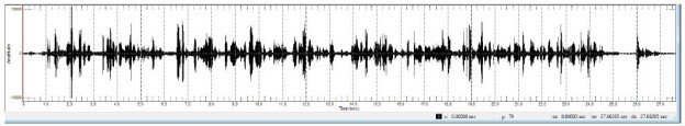
The waveforms in this study indicated a difference in prosody between the control group and foreign participants, which needs to be addressed when working with foreign accents. As noted, the 21 participant raters listened to the audiotapes of the paragraph readings by the individuals from different countries as well as those from the control group. The results of the data from the Multidimensional Voice Program show the difference in waveforms between the accent group and control group in terms of prosody. See Figures 1-3 for examples of prosody related to foreign accent: pitch variation, intensity, and pausing. The results of the data from the Multidimensional Voice Program were in accord with the raters’ prosody evaluation (pitch variation, intensity, and pausing appropriately).

In comparison to the control group, the above examples of the foreign accent group show reduced vocal intensity, limited pitch variation, and inappropriate pausing (choppy speech) in comparison to the control group whose waveforms indicate suitable pitch variation, pausing appropriately, sufficient intensity (Figures 4-6) which follow.

As noted above, the examples of the foreign accent group (Figures 1-3) show reduced vocal intensity, limited pitch variation, and inappropriate pausing, in comparison to the control group (Figures 4-6), where these areas of prosody indicate sufficient intensity, and both appropriate pausing and pitch variation. In sum, the figures relating to the two groups show prosody and voice differences between the control group and the accent group as observed in the waveforms.

fig 1

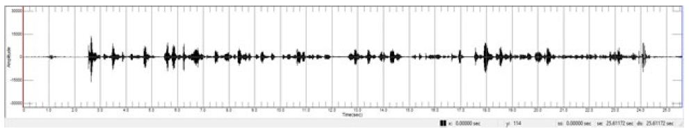
Figure 1: Foreign (African) Accent

fig 2

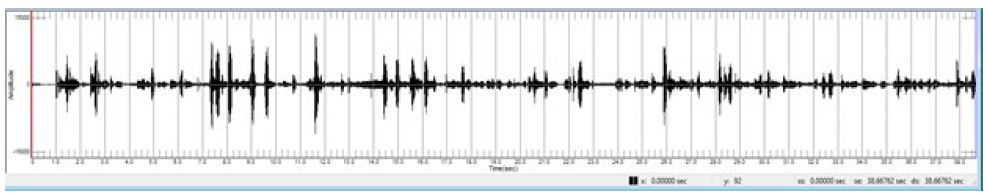
Figure 2: Foreign (Japanese) Accent

fig 3

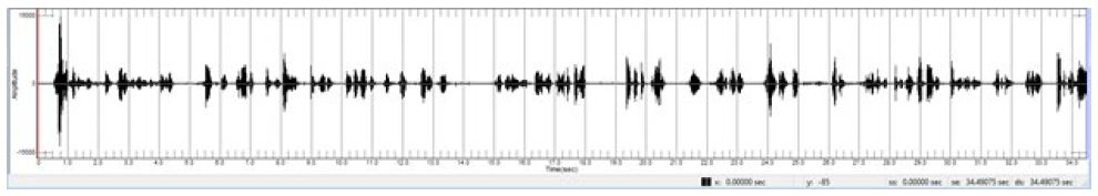
Figure 3: Foreign (Urdu) Accent

fig 4

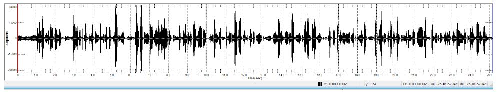
Figure 4: Control Group

fig 5

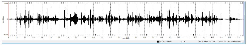
Figure 5: Control Group

fig 6

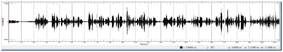
Figure 6: Control Group

Participant Raters’ Results

Seven raters from each of the following groups–professors, graduate, and undergraduate speech pathology students compared and listened to the recordings of both the participants and the control group. The raters evaluated the prosody of the two groups on a scale of 1 to 5, with 1 being within normal limits. They found the following characteristics in the accent group: excessive pausing, inappropriate pausing, monotone voice or limited pitch variation, choppy speech, prolonged speech, slow rate, too loud or too soft. These results appeared to confirm the data seen on the waveforms. According to the raters, the suprasegmentals which most negatively affected speech/voice production were the following from the highest to lowest degree of frequency.

Choppy Speech: Frequency: 198 (67.3%)

Pitch Variation (monotone): Frequency: 184 (62.6%)

Excessive Pausing Frequency: 146 (49.7%)-related to choppy speech

Speech Rate (too slow): Frequency: 135 (45.9%)

The characteristics found in the control group were all within regular limits, compared to the accent group. The waveforms on the instrument appeared aligned with the raters’ evaluations of the participants.

Questions Answered:

  1. In the present study, which suprasegmentals had the most negative effect on prosody on a scale of 1-5, with 5 being the most difficult?
  2. The participants had the most difficulty pausing appropriately and using pitch variation, resulting in choppy speech, a monotone voice, and speaking too slowly.

  3. Is there a difference in ratings among the three groups of raters, that is, the professors, the graduate students, and the undergraduate students, all of whom are in the department of Speech Communication Arts and Sciences?
  4. The three rater groups evaluated all the participants (both control and accent groups) and were consistent in their ratings regarding the above characteristics for the accent group: choppy speech production, monotone voice, speaking too slowly, and inappropriate pausing. The control group, however, demonstrated appropriate pausing, pitch variation, speech rate (prosody was consistently rated within normal limits).

  5. Which aspects of prosody were the least affected by accent, according to the raters?

The least affected aspects were loudness (intensity) and word stress, that is, for this group of participants.

Discussion

This study was undertaken to bring attention to problems with prosody and how the suprasegmentals of speech and voice (e.g., intonation, vocal intensity, rate and rhythm, stress) not used appropriately can have a negative effect on prosody and thus listener comprehension. Viewing the waveforms of the participants in comparison to the control group’s waveforms, it is obvious that the participants exhibit almost a flat waveform with very little pitch variation, which is how their speech was perceived by the raters who listened to their recordings. These suprasegmentals are important for listener comprehension of the content and to impart the value of prosody to the clients in terms of listener comprehension. The above findings highlight the importance of addressing suprasegmentals during voice and speech therapy for clients who have difficulty with prosody to increase the intelligibility of their speech.

It is possible that the suprasegmentals may not always be addressed in therapy, even though a negative effect on voice and speech may occur if not used correctly. Not addressing prosody, when necessary, can reduce progress in terms of obtaining the most positive outcome. Individuals with voice problems must learn how to use their voices without phonotrauma and work on the suprasegmentals as well (if needed) which can enhance voice, listener comprehension of the message, and meaning. Working on the suprasegmentals can also have a positive effect on speech production. That is, correcting one prosodic feature can have a positive effect on another feature. For example, reducing choppiness may increase pitch variation and improve the client’s use of voice, as well as listener comprehension. Excessively slow rate, lack of pitch variation, low vocal intensity, incorrect stress, can reduce the meaning of the information heard and deprive the vocal folds from being appropriately engaged (e.g., to change the pitch for meaning). Field (2005) [23], for example, wrote an initial first language study that showed misplacing stress (which involves how one uses the voice) in words can seriously impair speech intelligibility. As noted, Ben-David et al. (2016) found that prosody and semantics are integral as one has an influence on the other [11]. The authors note, however, that prosody has a greater impact on the emotional rating of speech in comparison to semantics, and voice often incorporates emotion.

As noted, studies by Tolhurst (1957), Picheny et al. (1986), Li and Loizou (2008), Smiljanic and Bradlow (2008), and Hazan and Baker (2011) showed that speakers demonstrate some control over the intelligibility of their speech by implementing various speaking styles to increase listeners’ understanding. The authors determined that improving the suprasegmental features (e.g., appropriate speech rate, more appropriate pausing, pitch variation, appropriate vocal intensity, and alteration of intonation patterns, without any vocal abuse) improved conversational speech perception. It is the present principal investigator’s experience that intelligibility and voice improve when incorporating appropriate prosody (suprasegmentals) during therapy.

Articulation, of course, is important in terms of both voice production and articulation, which can support voice. Inappropriate prosody, however, may reduce intelligibility even more than just producing a speech sound incorrectly. For example, if a person has a few speech sound substitutions (e.g., l/r, d/th, i/I (seat for sit)), the content may be understood. From the present research, however, when a person does not, for instance, connect words in sentences, speaks with a monotone voice, has significantly reduced vocal intensity, listeners may have greater difficulty understanding that person than one with a few related articulation errors. Additionally, when working with one suprasegmental, another suprasegmental can become incorporated in the therapy. For example, improving pitch variation and connected speech can lead to improvements in intensity, appropriate speech rate, and appropriate pausing; additionally, precise articulation can take effort off the larynx. Improvements in these aspects can be a part of voice therapy and very motivating to the client as voice is enhanced. Prosody also gives the individual an avenue to express him or herself more meaningfully. Grigos and Patel note that “there is evidence to suggest that children master the suprasegmental aspects of speech before segmental features” indicating that prosodic control appears concurrently with language development and has an influence on the production of early infant vocalizations and words [14].

Most of the speakers featured in the clips/tapes of the present study were chosen because each had detectable accents and prosodic difficulties. There were, however, two clips of people from other countries who were judged to have regular prosody and vocal production. These latter clips/tapes indicate that one can have an accent and maintain appropriate prosody and suprasegmentals to which all the raters in this study agreed. These clips are not shown in the article, but they are similar to the waveforms of the control group, indicating appropriate prosody.

All of the participants in the clips/tapes of the present study were chosen because each had detectable accents with prosodic difficulties. Two clips of participants from foreign countries, however, not shown in this article, were judged by the raters to have regular prosody and vocal production in line with those of the control group. These two clips indicate that one can have an accent and maintain or learn to speak with appropriate prosody and suprasegmentals.

The following authors summarize the importance of prosody and its suprasegmentals on the impact on voice: McCabe and Altman (2017) stress that prosody in speech/voice production is essential as it provides contextual meaning in speech in terms of the variation of frequency, rate, and tone [41]. Prosody gives layers of meaning beyond the word. It communicates emotional and social elements that may not always be expressed through words. Voice therapy can offer individuals with prosodic difficulty methods to improve their prosody and thus their communication. Furthermore, according to Schirmer (2010) [42], a speaker’s prosody contributes to “shaping a word’s affective representation in memory” and may produce attitude changes in listeners that can have a lasting effect on listener behavior.

Nakatani and Schaffer (1978) found that stress and rhythm in terms of prosody affect speech naturalness as well as intelligibility, or the ease with which speech can be understood [43]. The findings of Patel et al. (2011) suggest that fundamental frequency and intensity are integrated to sustain the contrast between stressed and unstressed words [44,45].

Limitations

This study was limited because the raters evaluated the accented speech of individuals (the participants from different countries) who all read the same paragraph aloud, the latter to obtain consistency, in terms of the content, for comparison. Additionally, the study incorporated a small number of individuals with accents (participants).

Conclusion

The findings of this research revealed that voice production, which involves prosody related to the physiological components of voice and speech (e.g., intonation, pausing appropriately, breath support, articulation), should be part of voice therapy since prosody has a significant effect on voice production and listener comprehension. A recording device needs to be incorporated in the sessions, so that the clients can hear their improvements.

Acknowledgments

I am grateful to Dr. Howard Spivak, statistician, for his very helpful input into this article; I also thank the Brooklyn College professors and students who participated in this study by rating the accent tape recordings. I appreciate Dr. Alla Chavarga’s assistance in summarizing and discussing the results. I am especially appreciative of the contributions and assistance of Deema Farraj, Brooklyn College student, for her excellent assistance on the computer, editing the manuscript, and insightful input into this study.

References

  1. Belyk M, Brown S (2014) Perception of affective and linguistic prosody: An ALE meta-analysis of neuroimaging studies. Soc Cogn Affect Neurosci 9: 1395-1403. [crossref]
  2. Wagner M, Watson DG (2010) Experimental and theoretical advances in prosody: A review. Lang Cogn Process 25: 905-945. [crossref]
  3. Mannel R (2007) Introduction to Prosody theories and models. Macquarie University.
  4. Steedman M (1991) Structure and intonation. Lang 67: 260-296.
  5. Munhall KG, Jones JA, Callan DE, Kuratate T, Vatikiotis-Bateson E (2004) Visual prosody and speech intelligibility: Head movement improves auditory speech perception. Psychol Sci 15: 133-137. [crossref]
  6. Paige DD, Rasinski T, Magpuri-Lavell T, et al. (2014) Interpreting the relationships among prosody, automaticity, accuracy, and silent reading comprehension in secondary students. J Lit Res 46: 123-156.
  7. Cutler A (1986) Forbear is a homophone: Lexical prosody does not constrain lexical access. Lang Speech 29: 201-220.
  8. Hahn LD (2004) Primary stress and intelligibility: Research to motivate the teaching of suprasegmentals. TESOL Quart 38: 201-223.
  9. Trofimovich PA (2016) Multidimensional scaling study of native and non-native listeners’ perception of second language speech. Percept Mot Skills 122: 470-489. [crossref]
  10. Wikimedia Foundation. (2021, December 15). Prosody (linguistics). Wikipedia. Retrieved December 15, 2021, from https://en.wikipedia.org/wiki/Prosody_(linguistics)
  11. Ben-David, BM, van Lieshou P (2016) Prosody and semantics are separate but not separable channels in the perception of emotional speech. Test for rating of emotions in speech. J Speech Lang Hear Res 59: 72-89. [crossref]
  12. Behrman A (2014) Segmental and prosodic approaches to accent management. Amer J Speech Lang Pathol 23: 546-561. [crossref]
  13. Klopfenstein M (2009) Interaction between prosody and intelligibility. Intl J Speech Lang Pathol 11: 325-331. [crossref]
  14. Grigos MI, Patel R (2007) Articular movement associated with the development of prosodic control in children. J Speech Lang Hear Res 50: 119-130. [crossref]
  15. Groen MA, Veenendaal NJ, Verhoeven L (2018) The role of prosody in reading comprehension: evidence from poor comprehenders. J Res in Read 42: 37-57.
  16. Felps D, Bortfeld H, Gutierrez-Osuna R (2008) Prosodic and segmental factors in foreign-accent conversion [PDF file]. Department of Computer Science, Texas A&M University, Technical Report tamu-cs-tr-2008-7-1.
  17. Bruce C, To CT, Newton C (2012) Accent on communication: The impact of regional and foreign accent on comprehension in adults with aphasia. Disabil Rehabil 34: 1024-1029. [crossref]
  18. Anderson-Hsieh J, Johnson R, Koehler K (1992) The relationship between native speaker judgements of non-native pronunciation and deviance in segmentals, prosody and syllable structure. Lang Learn 42: 529-555.
  19. Amano-Kusumoto A, Hosom JP (2011) A review of research on speech intelligibility and correlations with acoustic features [PDF file]. Center for Spoken Language Understanding (CSLU) Tech Rept 001: 1-16.
  20. Jung MY (2010) The intelligibility and comprehensibility of world English’s to non-native speakers. Pan-Pacific Assoc Appl Linguis 14: 141-163.
  21. Levi SV, Winters SV, Pisoni DB (2007) Speaker-independent factors affecting the perception of foreign accent in a second language. J Acoust Soc Amer 121: 2327-2338. [crossref]
  22. Derwing T, Munro MJ, Wiebe G (1998) Evidence in favor of abroad framework for pronunciation instruction. Lang Learn 48: 393-410.
  23. Field J (2005) Intelligibility and the listener: The role of lexical stress. TESOL Quart 39: 399-423.
  24. Lepage A, Busà MG (2014) Intelligibility of English L 2: The effects of incorrect word stress placement and incorrect vowel reduction in the speech of French and Italian learners of English [PDF file]. Proceedings of the International Symposium on the Acquisition of Second Language Speech Concordia Working Papers in Applied Linguistics 5: 387-400.
  25. Bond ZS, Small LH (1983) Voicing, vowel, and stress mispronunciations in continuous speech. Percept Psychophys 34: 470-474.
  26. Grosjean F, Gee JP (1987) Prosodic structure and spoken word recognition. Cogn 25: 135-155. [crossref]
  27. Cutler A, Clifton C Jr (1984) The use of prosodic information in word recognition. In H. Bouma & D. G. Bouwhuis (Eds.), Attention and performance X: Control of language processes. Hillsdale, NJ: Erlbaum 183-196.
  28. Yenkimaleki M, Heuven VJ (2018) The effect of teaching prosody awareness on interpreting performance: An experimental study of consecutive interpreting from English into Farsi. Perspect 26: 84-99.
  29. Sapir S, Pawlas AA, Ramig LO, Hinds SL, Countryman S, et al. (2001) Effects of Intensive Phonatory-Respiratory Treatment (LSVT) on voice in two individuals with multiple sclerosis. J Med Speech Lang Pathol 9: 141-151. [crossref]
  30. Tolhurst G-C (1957) Effects of duration and articulation changes on intelligibility, word reception and listener preference. J Speech Hear Disord 22: 328-334. [crossref]
  31. Picheny MA, Durlach NI, Braida LD (1986) speaking clearly for the hard of hearing II: Acoustic characteristics of clear and conversational speech. J Speech Hear Res 29: 434-446. [crossref]
  32. Li N, Loizou P (2008) Factors influencing intelligibility of ideal binary-masked speech: Implications for noise reduction. J Acoust Soc Amer 123: 2287-2294. [crossref]
  33. Smiljanic´ R, Bradlow A (2008) Speaking and hearing clearly: Talker and listener factors in speaking style changes. Lang Linguist Compass 3: 236-264. [crossref]
  34. Hazan V, Baker R (2011) Acoustic-phonetic characteristics of speech produced with communicative intent to counter adverse listening conditions. J Acoust Soc Amer 130: 2139-2152. [crossref]
  35. Dreher JJ, O’Neill JJ (1957) Effects of ambient noise on speaker intelligibility for words and phrases. J Acoust Soc Amer 29: 1320-1323. [crossref]
  36. Summers WV, Pisoni DB, Bernacki RH, et al. (1988) Effects of noise on speech production: Acoustical and perceptual analyses. J Acoust Soc Amer 84: 917-928. [crossref]
  37. Ramig LO, Sapir S, Fox C, Countryman S (2001) Changes in vocal loudness following intensive voice treatment (LSVT) in individuals with Parkinson’s disease: a comparison with untreated patients and normal age-matched controls. Mov Disord 16: 79-83. [crossref]
  38. Patel R, Hustad, KC, Connaghan KP, et al. (2012) Relationship between prosody and intelligibility in children with dysarthria. J Med Speech Lang Pathol 20: 17. [crossref]
  39. Koschanski G, Grabe E, Colman J, et al. (2005) Loudness predicts prominence: fundamental frequency lends little. J Acoust Soc Amer 118: 1038-1054. [crossref]
  40. Akil F, Yollu, Umur U, Ozturk O., Yener, M. 10: 2017.
  41. McCabe DJ, Altman KW (2017) Prosody: An overview and applications to voice therapy. Glob J Oto 7: 555719.
  42. Schirmer A (2010) Mark my words: Tone of voice changes affective word representations in memory. PLoS One 5: e9080. [crossref]
  43. Nakatani LH, Schaffer JA (1978) Hearing “words” without words: prosodic cues for word perception. J Acoust Soc Am 63: 234-245. [crossref]
  44. Patel R, Niziolek C, Reilly K, Guenther FH (2011) Prosodic adaptations to pitch perturbation in running speech. J Speech Lang Hear Res 54: 1051-159. [crossref]
  45. Cooper N, Cutler A, Wales R (2002) Constraints of lexical stress on lexical access in English: Evidence from native and non-native listeners. Lang Speech 45: 207-228. [crossref]
fig 1

Corporate Reputation of the Schools and Faculties of Social Work around Training by Competences of Intellectual Capital

DOI: 10.31038/ASMHS.2022615

Abstract

Corporate governance as a knowledge management system has been approached from the organizational reputation as a result of alliances with institutions. In the health sector, the demand for quality service has led to a system of professional internships and deregulated social service in which the image of the universities and health centers involved is in question. The objective of the present work was to contrast a model for the study of the phenomenon with the intention of specifying the relationships between variables. A non-experimental, exploratory and cross-sectional study was carried out with a non-probabilistic and intentional sample of 1018 administrators, professionals and students from the health sector. It was found that the case monitoring factor reflected the image of universities as trainers of intellectual capital by competencies. In relation to the consulted literature, lines of research are proposed to specify the model.

Keywords

Corporation, Training, Reputation, Competencies, Responsibility

Introduction

Within the framework of human development, health is a fundamental item for observing the corporate reputation of the School and Faculties of Social Work, understanding that it is about expectations of users, administrators, professionals and students regarding the quality of service public and depending on spending on prevention and care [1].

Mexico occupies the third last place in terms of health, public, social works, prepayments, out-of-pocket expenses, among other items related to prevention and care, which add up to 6% of the Gross Domestic Product (GDP) [2].

The corporate reputation of Public Health Institutions (ISP) and Higher Education Institutions (HEI) can be established if spending is associated with user expectations [3]. The 2015 economic census and the survey on the quality of public services note a medium and low performance of public centers and hospitals [4].

The average expenditure on medications and medical consultation is in second place once food and personal hydration have been paid for [5].

If it is considered that spending on hydration accounts for 20% of income for the popular, marginalized and excluded sectors, the prevention of diseases transmitted by hydration, when associated with spending on professional medical care, as well as on medicines, accounts for 40% for areas peri-urban areas from where they move to central cities to work, study or seek employment and education opportunities [6].

Regarding the formation of intellectual capital, Mexico occupies the penultimate place in the OECD in terms of adolescents and young people who do not have access to study or work, which is added to 14% of expectations of low quality of public education [6].

It is possible to infer that the reputation of corporate governance, health and medical assistance institutions, as well as the formation of intellectual capital, are on the decline, and a diagnosis of the HEIs that train health professionals is urgent, among which are the Schools and Faculties of Social Work [7].

Corporate Reputation Theory

Figure 1 shows the theoretical and conceptual frameworks that explain corporate reputation understood as the expectations of employees, directors and clients alluding to effective responses to environmental contingencies, context requirements or social demands [8].

fig 1

Figure 1: Corporate Reputation Theory.
TPI = Stakeholder Theory, TLT = Transformative Leadership Theory, TDP = Prospective Decision Theory: NM = Norms, VS = Values, CR = Beliefs, AC = Attitudes, PC = Perceptions, IN = Intentions, CM = Behaviors
Source: Self made.

The Stakeholders Theory warns that employees, shareholders, leaders and clients not only have a direct and significant participation in the company but also confront peripheral actors such as protesters, the media or institutions that seek to counteract the prestige of the company. institution in order to increase its credibility and position itself in the market [9].

Around the conflict between the interested parties and external factors to public health institutions, corporate governance is created as a shield of empathy, trust, commitment and satisfaction that guarantees the union of shareholders, leaders, employees and clients against the environmental threats, but it is in terms of reputation and prestige that differences and similarities between internal and external actors are resolved [10].

However, it is known that adhocratic organizational cultures, as well as traditional leadership, promote internal asymmetries in the face of external threats to the detriment of corporate reputation and prestige [11].

It will be the transforming cultures and leaderships who will manage knowledge to establish competitive advantages in the formation of intangible assets such as training and training of intellectual capital, future artificial and emotional intelligence cadres that will be decisive in entrepreneurship and innovation [12].

In such a context and scenario of cultures and transformative leaderships, decision makers are oriented towards vision and prospective missions as a second competitive advantage coupled with the formation of intangible assets [13].

This is the case of strategic alliances and knowledge management between HEIs and community, public or collective health institutions where systems of professional practices and social service are established in order to train future health professionals, among whom are social workers [14].

The Theory of Prospective Decisions posits that organizations prefer intentions and decisions aimed at maximizing risks and profits over strategies to reduce risks and reduce benefits [15].

In the case of the formation of human capital, a prospective decision suggests risks in the formation with high benefits in the prestige and reputation of the HEI or the health center. These are early professional internship strategies for students who have not covered the minimum credits, or social services who have not accredited seminars or basic subjects [16].

Another aspect to consider refers to the lack of resources for the hiring of professionals and the employment of interns and social workers to remedy the deficit of attention to public health services, or their use in health promotion, campaigns of prevention or allocation of medications to vulnerable groups [17].

In sum, stakeholder theory, transformational leadership theory, and prospective decision theory suggest the need for a comprehensive, specific, and up-to-date diagnosis of corporate governance, reputation, and institutional prestige, as well as expectations. of shareholders, directors, talents and users of HEIs in strategic alliances with collective health centers [18].

Given that corporate governance in general and training reputation and prestige in particular are little studied objects in the HEIs where the Schools and Faculties of Social Work are located, it is necessary to carry out a comprehensive diagnosis of the skills of future professionals with the purpose of inferring the intangible value of public universities in strategic alliances with health centers, as well as their differences and similarities in terms of professional skills [19].

Formulation

Will there be significant differences between HEIs in central, western and northern Mexico in terms of training skills for health services?

Hypothesis

Null Hypothesis

There will be significant differences between the HEIs studied with respect to the professional training of skills for public health services

Alternate Hypothesis

There will be no significant differences between the study HEIs regarding the professional training of skills for public health services

Method

An exploratory study was carried out with a sample of students, directors and professionals of the Social Work of Health in HEIs in the center, west and northeast of Mexico, considering their affiliation to a public university with an internship system in health centers, accreditation of the minimum percentage for social service and professional practices (Table 1).

Table 1: Descriptions of the study sample


Students

professionals Administrative Sex Age

Entry

UAEH

93

37 14 Female(45%) Male(55%) M=25.3 SD=3.89

M=$346.1 SD=$9.3

UAEM

91

3. 4 12 Female(57%) Male(43%) M=29.8 SD=4.78

M=342.1 DE=$8.3

UAEMEX

90

33 eleven Female(67%) Male(33%) M=27.3 SD=3.80

M=$432.1 SD=$7.1

UAM

89

30 10 Female(49%) Male(51%) M=28.6 SD=2.79

M=367.2 DE=$8.2

UAQ

87

29 9 Female(44%) Male(56%) M=36.1 SD=1.32

M=$342.1 SD=9.3

UAT

85

27 8 Female(52%) Male(48%) M=33.1 SD=1.67

M=$396.1 SD=$10.4

UNAM

84

25 7 Female(43%) Male(57%) M=37.1 SD=4.35

M=$354.1 SD=71.1

USON

83

24 6 Female(60%) Male(40%) M=39.8 SD=2.34

M=$359.8 SD=$5.4

Source: Prepared with study data

The Corporate Reputation Scale (ERC-28) was built based on items selected from the consulted literature, which measured expectations of the parties involved regarding objectives, tasks and goals related to entrepreneurial and innovative knowledge skills such as collaborative work. professional (Table 2).

Table 2: Construction of the ERC-28

Competence

Definition Indicator Coding

Interpretation

Accompaniment It refers to an emotional ability to establish a bond of social, family or personal support with the user of the health service (Vaquero, 2012) Data relating to cases of self-medication or self-harm 0=“not at all likely” to 5=“quite likely” High scores refer to a corporate governance focused on the reputation and professional training prestige of the accompaniment
Accession It refers to the ability to motivate the user to use the health service in terms of consultation requests, medications and advice. (Kolade, Olakkeke, & Omotayo, 2014) (Data referring to the cases of rehabilitation and desertion to treatments 0=“not at all likely” to 5=“quite likely” High scores refer to a corporate governance focused on the reputation and professional training prestige of adherence to treatment
Advisory It refers to an ability to establish effective and accessible processing routes for health service users (Rondeaeu, 2017) Data alluding to the time of delay in each of the phases of the health service from the request for care to the rehabilitation 0=“not at all likely” to 5=“quite likely” High scores refer to a corporate governance focused on the reputation and professional training prestige of the management consultancy
Interview It refers to an ability to establish empathy with the user of health services, their needs, shortcomings and opportunities for a risk-free life (Olajide, 2014) Data alluding to the user’s detachment and trust towards health professionals, bureaucracy and administrative managers 0=“not at all likely” to 5=“quite likely” High scores refer to a corporate governance focused on the reputation and professional training prestige of the diagnostic interview
Mediation It refers to an ability to reduce differences and conflicts, as well as to establish points of agreement between the parties (Kelinde, 2012). Data related to conflicts and conciliations 0=“not at all likely” to 5=“quite likely” High scores refer to a corporate governance focused on the reputation and professional training prestige of conflict mediation
Promotion It refers to an ability to disseminate data and prevention strategies for illnesses and accidents for a risk-free life (Jinfeng, Runtian, & Quian, 2014). Data alluding to illnesses and accidents that affect occupational, emotional or biophysical health 0=“not at all likely” to 5=“quite likely” High scores refer to a corporate governance focused on the professional training reputation and prestige of health promotion
Follow-up It refers to an ability to establish parameters of quality of care in terms of satisfaction of the user of the health service (Melero and López, 2017) Data alluding to the quality of care and customer satisfaction 0=“not at all likely” to 5=“quite likely” High scores refer to a corporate governance focused on the reputation and professional training prestige of case monitoring

Source: Self made

The surveys were carried out in the facilities of the HEIs and health centers with a prior written guarantee of confidentiality, anonymity and non-affectation of the results. The information was processed in the Statistical Package for Social Sciences (SPSS version 25.0).

Reliability and validity analyzes of the instrument, hypothesis tests for differences between groups, as well as correlations, general linear models and structural equation models were carried out to establish the trajectories of dependency relationships between the variables and indicators of the ERC-15.

The following parameters were estimated: 1) mean, 2) standard deviation, 3) bias, 4) kurtosis, 5) asymmetry, 6) Crombach ‘s alpha , 7) Student’s t – test, 8) analysis of variance F-test, 9) KMO test, 10) Bartlett test, 11) Pearson correlations, 12) beta regressions, 13) goodness of fit, and 14) residuals.

Results

Table 3 shows the statistical properties of the ERC-28 in which reliability alpha values higher than the indispensable minimum of .700 are observed for the general instrument (alpha of .780) and the subscales (respective alphas of .776; .781); .756; .790; .719; .750; .732).

Table 3: Descriptives of the CKD-28

R

M D yes C TO F1 F2 F3 F4 F5 F6 F7
R1 1.32 ,821 1.59 1.54 ,782

,360

R2

1.25 .943 1.65 1.65 ,793 .469
R3 1.43 .972 1.67 1.29 ,784

,540

R4

1.39 ,784 1.83 1.03 ,763 .457
R5 4.37 1.30 1.75 1.17 ,751 ,564

R6

4.21 1.21 1.60 1.81 ,759 .439
R7 4.21 1.43 1.73 1.43 ,783 ,406

R8

4.43 1.46 1.83 1.12 .752 .326
R9 3.45 ,864 1.95 1.14 ,714 .435

R10

3.50 .975 1.61 1.03 ,750 .329
R11 3.56 ,931 1.68 1.05 ,762 .438

R12

3.52 ,831 1.92 1.24 ,741 ,384
R13 1.39 4.36 1.61 1.16 ,739 .438

R14

1.45 4.18 1.74 1.46 .752 .548
R15 1.46 4.39 1.82 1.67 ,751 ,324

R16

1.21 4.39 1.93 1.02 ,754 .455
R17 4.56 1.52 1.62 1.13 ,749 .421

R18

4.35 1.48 1.79 1.15 ,731 ,486
R19 4.25 1.32 1.73 1.15 ,743 ,340

R20

4.67 1.14 1.82 1.45 ,724 ,389
R21 2.46 2.35 1.70 1.24 ,743 ,398

R22

2.57 2.14 1.82 1.13 ,763 .412
R23 2.54 2.43 1.71 1.15 ,716

,378

R24

2.14 2.87 1.94 1.17 ,730 ,420
R25 4.50 ,871 1.84 1.06 ,753

.423

R26

4.67 .943 1.74 1.09 ,726 ,379
R27 4.18 ,921 1.92 1.17 ,743

.421

R28

4.39 .953 1.75 1.18 ,750 .347

R=Reactive, M=Mean, D=Standard Deviation, S=Skew, C=Kurtosis, A=Alpha removing the value of the item. Adequacy (KMO=.732), Sphericity ⌠X2=23.6 (5df) p=.000⌡Extraction method: principal axes, rotation: promax. F1=Accompaniment (18% of the total variance explained), F2=Adherence (17% of the total variance explained), F3=Advice (15% of the total variance explained), F4=Interview (13% of the total variance explained), F5=Mediation (11% of the total variance explained), F6=Promotion (8% of the total variance explained), F7=Follow-up (5% of the total variance explained). All items are answered with one of five options: 0=“not at all likely” to 5=“quite likely”.
Source: Self made.

The correlation matrix shows discriminant validity by including values close to zero, but the covariance matrix warns of the possibility of excluding other factors due to values close to unity (Table 4).

Table 4: Correlation and covariance matrices


F1

F2 F3 F4 F5 F6 F7 F1 F2 F3 F4 F5 F6

F7

F1

1,000

1.59
F2

2. 3. 4*

1,000 ,743

1.83

F3

,313

.246 1,000 ,831 .674

1.79

F4

.435*

,318 .239 1,000 .932 ,756 ,794 1.68
F5

,294

.268** .217*** .246 1,000 ,748 .865 ,874 ,608 1.50
F6

.105

.106 .443 .128 .319* 1,000 ,693 ,608 ,792 ,704 ,893

1.68

F7

,392

.146 .329 .236* .246 .246 1,000 ,761 .642 .775 .872 ,768 ,798

1.72

F1=Accompaniment, F2=Adhesion, F3=Counseling, F4=Interview, F5=Mediation, F6=Promotion, F7=Follow-up: * p <.01; ** p <.001; *** p <.0001.
Source: Prepared with study data.

The sum of the percentages of explained variance (87%) revealed the preponderance of seven factors that can converge in a common factor of the second order (Figure 2).

figure 2

Figure 2: Structural model of trajectories of dependency and reflective relationships.
C = Corporate Reputation: F1 = Accompaniment, F2 = Adhesion, F3 = Advice, F4 = Interview, F5 = Mediation, F6 = Promotion, F7 = Follow-up; r = Reactive, d = Disturbance, e = Measurement error
Source: Prepared with study data.

The second-order factor related to corporate reputation included the eight first-order factors established from the review of the literature. The structural model included as a reflective factor the competence of case follow-up (.67). In other words, the corporate reputation of the social work public service is centered on the academic and administrative training of monitoring skills rather than on the skills of support, adherence, advice, interview, mediation and health promotion.

The fit and residual parameters ⌠X2=345.23 (56df) p=.008; GFI=.997; CFI=.990; NFI=.995; RMSEA=.009; RMR=.007⌡ suggest the non-rejection of the null hypothesis regarding the differences between the competencies reviewed in the literature with respect to the structural model.

Discussion

The present work has established the contrast of a model for the study of seven exploratory factorial dimensions of corporate reputation in HEIs in central, western and northern Mexico, although the type of non-experimental study, the type of intentional selection and the type of exploratory factor analysis limit the results to the study sample, suggesting lines of research and intervention related to the follow-up of cases as a factor reflecting the organizational phenomenon.

[1,3,19-28] contrasted models to observe corporate reputation in its reflective dimensions: 1) aversive or entrepreneurship and real innovation of the organization; 3) responsive or ecological footprint of the organizational production; 3) prospective or expected future of the organization, concluding that organizations seem to go through a process that goes from aversion to risks indicated by cultures, leaderships and adhocratic climates towards a propensity for the future indicated by cultures, leaderships and conciliatory climates of the organization image of collaborative knowledge networks.

In the present work, an exploratory model of seven factors has been contrasted in which the institutional follow-up of user cases is the hallmark of HEIs that, in alliance with health centers, train future operational-administrative cadres. The factor reflecting the follow-up of cases is part of the dimension of responsiveness cited in the literature.

Therefore, it is necessary to: a) build an instrument to explore the indicators of the responsive dimension as a preponderant factor of corporate reputation; b) contrast an exploratory model in order to establish the convergent and divergent validity of the scale; c) associate the responsive dimension with the aversive and prospective dimensions in order to build an integral model.

Conclusion

The present work has contrasted a model of seven dimensions reflecting the reputation of HEIs specialized in Social Work in Health, which is centered on the competence of case follow-up. In relation to the findings reported in the literature, the model can be specified in the responsive dimension, this being the one that would explain the distance or closeness that the respondents refer to as the competitive advantage of their academic and professional training.

References

  1. Bustos JM, Ganga F, Llamas B, Juárez M (2018) Contrast of a prospective decision model in implications for a university governance of sustainability. Margin 89: 1-16.
  2. Garcia C (2018a) Reliability and validity of an instrument that measures knowledge management in a public university in central Mexico. Tlatemoani 27: 285-304.
  3. Sánchez R, Villegas E, Sánchez A, Espinosa F, García C (2018) Model for the study of organizational clarity and corporate social responsibility. Synchrony 22: 467-483.
  4. García C, Espinosa F, Carreón J (2018) Model of intangible assets and capitals in organizations. International Journal of Research in Humanities and Social Studies 5: 1-12.
  5. Garcia C (2018b) Interpretations of knowledge management discourses for the understanding of narratives of innovative entrepreneurship. Inclusions 5: 96-111.
  6. Garcia C, Martinez E, Rivera PE (2018) Labor flexibility in higher education. Inclusions 5: 51-69.
  7. Villegas E, Garcia C, Hernandez TJ (2018) Establishment of a science and technology policy for the incubation of innovative knowledge micro-enterprises. Inclusions 5: 19-26.
  8. Rubio A, Jiménez IC, Mercado C (2017) Online corporate reputation in the hotel industry: The case of tripadvisor. Market Economic & Business Journal 48: 579-593.
  9. Perrini F, Vurro C (2013) Stakeholders orientation and corporate reputation: A quantitative study on US companies. Emerging Issues in Management 1: 53-65.
  10. Babie V, Arslanagic M, Mehic E (2013) Importance of internal marketing for service companies’ corporate reputation and customer satisfaction. Journal of Business Administration research 12: 49-57.
  11. Barnnett M, Jermier JM, Lafferty BA (2006) Corporate reputation: The definitional landscape. Corporate Population Review 9: 26-38.
  12. Blajer A (2014) Corporate reputation and economic performance the evidence from Poland. Economic & Sociology 7: 194-207.
  13. Cariton R, Moura RC (2012) The impact of R&D intensity on corporate reputation: interaction effect of motivation with high social benefit. Intangible Capital 8: 216-238.
  14. Beheshtifar M, Korouki A (2013) Reputation: An important component of corporation value. International Journal of Academic Research in Business & Social Science 3: 15-20.
  15. Casimiro MC, Matos A (2017) The impact of corporate reputation in a dairy company. Business & Economics Journal 8: 1-11.
  16. Marquina P, Arellano R, Velázquez I (2014) A new approach for measuring corporate reputation. Administration 54: 53-66.
  17. Martinez P, Rodriguez I (2013) Intellectual capital and relational capital: The role of sustainability in developing corporate reputation. Intangible Capital 9: 262-280.
  18. Fiala R, Prokov M (2013) The relationships among reputation, inter-organizational trust and alliance performance. University Act 99: 899-908.
  19. Hernández TJ, Sánchez A, Espinosa F, Sánchez R, García C (2018) Model of lucidity, entrepreneurship and innovation in coffee microenterprises in central Mexico. Eureka 15: 96-107.
  20. Garcia C, Rivera PE, Martinez E (2018) Institutionalist academic culture in Cuernavaca, Modelos (Mexico). Inclusions, 5: 84-96.
  21. Garcia C, Rivera PE, Martinez E (2018) Institutionalist academic culture in Cuernavaca, Modelos (Mexico). Inclusions, 5: 84-96.
  22. Jinfeng L, Runtian J, Quian C (2014) Antecedents of corporate reputation and customer citizenship behavior. International Business & Management 9: 128-132.
  23. Kelinde O (2012) Organizational culture and its corporate image: A model juxtaposition. Business & Management Research 1: 121-132.
  24. Kolade OJ, Olakkeke O, Omotayo O (2014) Organizational cityzenship behavior, hospital corporate image and performance. Journal of Competitiveness 6: 36-49.
  25. Melero I, Lopez ML (2017) Identifying link between corporate social responsibility and reputation: Some considerations family firms. Journal Evolutionary Studies in Business 2: 191-230.
  26. Olajide FS (2014) Corporate social responsibility practices and stakeholders’ expectations. Research in Business & Management 1: 13-31.
  27. Rondeau KV (2017) The impact of world ranking systems on graduate schools of business: promoting the manipulation of image over the management of substance. World Journal of Education 7: 62-73.
  28. Cowboy A (2012) Online reputation in the framework of corporate communication. An insight into research trends and career prospects. Communication 3: 49-63.
fig 2

Spatial Variability of Elemental Concentrations in Three Marine Fishes along the Coastal Waters of Andhra Pradesh

DOI: 10.31038/JPPR.2022512

Abstract

In the presented study, three different marine fish species were collected from four locations along the coastal waters of Andhra Pradesh. The samples were analysed using Hand-held XRF. Concentrations of ten elements (As, Cd, Cu, Fe, Mn, Se, Zn, Ca, K and Mg) were quantified in muscle, liver and gill tissues of Rastrelliger kanagurta, Euthynnnus affinis and Saurida tumbil collected from Visakhapatnam harbour, Kakinada harbour, Pudimadaka and Bheemili. There was a clear spatial variation in the concentration of elements collected from different locations. However, significant differences in elemental concentrations among the three studied species and tissues were observed and these may be related to different accumulation patterns of the species. The results showed that concentrations of As and Cd were above the threshold limits. However, the exposure for the population depends on their dietary habits and continued exposure to the heavy metals may cause adverse effects.

Keywords

Marine fish, HHXRF, Heavy metal

Introduction

During the last few years, aquatic ecosystems have been affected by various types of contaminations due to garbage and effluents delivering by different sectors like domestic, agricultural, commercial, and pharmaceutical and other industrial activities of human beings living around the coastal lines. In recent years [1], much attention has been paid to study about health benefits of essential elements (Fe, Zn, Cu, Mn) derived from fishes of the marine environment due to consumption of sea fishes and change in their concentration due to pollution impact causing associated health hazards besides the accumulation of non-essential elements or heavy metals (Hg, Cd, Pb) in the fishes. Nutritionists consider fish products to be a major source of quality protein, vitamins, minerals and long-chain polyunsaturated fatty acids (omega-3), docosahexaenoic acid (DHA) and also contain organic and inorganic micronutrients like vitamin D, selenium etc. [2]. Fishes are recommended mainly to the elderly, infant’s brain and nerves function, cardiac patients i.e., abnormal heart strokes and those with digestive problems due to their reduced energy levels and higher mineral content [3]. Consuming fish may decrease the risk of depression, Alzheimer’s disease, arthritis and diabetes etc. On the other hand, Toxicologists tend to regard aquatic pollution as a major vector for non-essential elements like Hg, Cd, Pb accumulation [4]. These elements are mainly present in marine environments due to industrial wastewater loads, soil erosion, municipal sewage discharges from rural and urban areas, agricultural land runoff [5]. Natural phenomena such as earthquakes, landslides, tornadoes, cyclones, and weathering of rocks also contribute towards heavy elements contribution for pollution. The contaminated water is the major source of elements bioaccumulation in the various vital organs (Liver, Kidney, gills) of the fish. Discharge of agricultural wastes like agrochemicals, Organic matter and industrial wastewater without pre-treatment into lakes, rivers and oceans resulting in an increase of non-essential elemental concentration in such water environments exhibiting damage on aquatic life [6]. Elemental pollutants as particles, elemental ions; inorganic and organic compounds in rivers and oceans also damage aquatic life [7,8]. Heavy elements, which especially collected in the organs of fishes, such as spleen and kidneys may be transmitted and accumulated in human organs through their consumption [9] and can cause a risk of kidney, brain and nervous system damage to human beings. Therefore, the introduction of non-essential elements into the food chain threatens human health and also to aquatic life. Essential elements may also become toxic to the human body if their intake is higher than the standard values of WHO [10].

The consumption of fish is significant for human beings living in coastal areas like Visakhapatnam and constitutes an important component in the intake of food items. Hence, continuous monitoring and analysing elemental concentration levels in fish belong to coastal areas became vital to understand the pollution impact on human beings those who consume frequently or regularly. Research on the detection of elements in fishes of these coastal areas is important because elemental concentration could cause growth disorders, reproductive disorders, immune suppression and histopathological alteration in the gills, kidney, liver and skin, as well as abnormalities in fish bones [11]. The health hazards associated with the consumption of contaminated fishes are up to 20-40 times greater than those associated with contaminated drinking water [12]. This is because fish have the ability to contain elemental concentration up to ten times higher than the observed environmental value [13]. Thus, fish may be considered biological indicators of elemental pollution and as a potential risk factor if contaminated fish are consumed by human beings. Absorption of elemental ions takes place through the skin, gills and digestive tract of fishes, which are transmitted to other parts of the body through the blood [14]. Muscles have been widely analysed for elemental concentration as they constitute the most edible portion of fish that poses a risk to human health who consumes them [15]. However, the liver, gills and kidneys collect the elements more effectively than the muscles since they are active metabolic tissues and primary organs for accumulating the majority of elements in fish [16]. The concentration level of elements in the gills indicate their concentration presented in the water in which the fish are found, and the liver’s concentration represents the retention of the elements, whereas the muscle is not regarded to be active tissue in the accumulation of elements [17]. Many organizations like the United States Food and Drug Administration (USFDA), the Food and Agriculture Organization (FAO) and the World Health Organization (WHO) have established limitations for human consumption of trace elements. The FAO/WHO Committee on Food Additives has set the provisional values of tolerable weekly intake (PTWI) and the dietary intakes of food additives and certain food contaminants. These specific values are significant for the safety levels of these elements in humans [18].

Materials and Methods

Samples Collection and Preparation

In the present study, three marine fishes commonly consuming by the people of Andhra Pradesh namely (Rastrelliger kanagurta (22-24 cm, TL), Euthynnus affinis (28-32 cm, TL) and Saurida tumbil (30-34 cm, TL) were collected freshly from four locations of coastal waters namely Visakhapatnam harbour (Geographical coordinates (17.6958° N, 83.3025° E), Kakinada harbour (16°58′30″N, 82°16′44″E), Pudimadaka fish landing centre (17.4927° N, 83.0028° E) and Bheemili fish landing centre (17.890382°N 83.455465°E). The sample collection areas along the coastal waters of Andhra Pradesh are shown in Figure 1. Photographs of the collected marine fishes belong to the Visakhapatnam harbour is presented in Figure 2. These fishes were individually packaged into polythene bags, stored in an ice box and brought to the laboratory. The selected species were collected three times during the winter season. The collected fishes were washed with distilled water and carefully dissected to obtain the muscle, gills and liver of the fish; subjected for determination of elemental concentrations accumulated in the respective parts. These samples were then kept at around -20°C in a deep freezer overnight in the laboratory. The frozen samples were lyophilized in a microprocessor-controlled freezing method. The lyophilization works at around -50°C which absorbs water molecules from the samples, drains off the samples making them completely dry. Then the dried specimens were ground using agate mortar and pestle to obtain fine powder with minimal contamination. The samples were kept separately with unique identification number in airtight packets.

fig 1

Figure 1: Sample collection areas along the coastal waters of Andhra Pradesh

fig 2

Figure 2: Fish Samples collected at Vishakapatnam fishing harbour

Experimental Method

The experimental work was carried out in BARC (Division of Nuclear Physics), Mumbai with Hand-held XRF (HHXRF) technique. In the XRF spectrometer, samples were excited by the X-rays emanating from an X-ray tube (Rh X-ray tube) having enough energy for ejecting electrons from various inner shells belonging to the atoms in the specimen. The vacancies in the inner shells of atoms are then occupied by electrons coming from the outer shells of the atoms causing the emission of characteristic X-rays; conventionally it can be referred to as X-ray fluorescence (XRF). In HHXRF, a silicon drift detector (SDD) was employed for the measurement of X-ray energies. The Silicon Drift Detector (SDD) contains graphene window that enables the detection of low Z elements (Al, S and P). These low Z elements usually cannot be detected by the conventional XRF system which uses a beryllium window. The powdered samples were placed in a cubic box and irradiated by Rhodium X-ray tube. Spectrum has been obtained for each sample in twenty seconds. The energy of the beams used for beam 1 is between 12 and 36 keV, whereas for beam 2, it varies between 0 to 12 KeV [19]. The HHXRF experimental set-up is as shown in Figure 3. The validity of the HHXRF set up was performed by analyzing Certified reference material (CRM) obtained from European Commision – Joint Research Centre, Institute for Reference Materials and Measurements – (ERMBB422 – Fish muscle) – was used for quantification of the elements and verifying the reliability of the data obtained by the present system.

fig 3

Figure 3: HHXRF set up

Results and Discussion

Concentrations of accumulated elements namely As, Cd, Cu, Fe, Mn, Se, Zn, Ca, K and Mg in different tissues belong to the fishes collected from four different locations are determined by using the obtained spectra. The observed results relating to the fishes collected from Visakhapatnam fishing harbour are compared with those collected from Kakinada fishing harbour, Pudimadaka, Bheemili as displayed in the Table 1. There is a clear spatial variation in the concentration of elements collected from different locations, however significant differences in elemental concentrations among the three studied species are observed; which may be related to different accumulation patterns of the species. The obtained XRF spectrum of the certified reference material (ERMBB422) is shown in Figure 4. The correlation coefficients among the evaluated average concentration values of various elements observed due to the three species are computed and shown in Tables 2-4.

Table 1: Concentrations of elements present in three different fish species collected at four locations

Element

Species Tissue Visakhapatnam Kakinada Pudimadaka

Bheemili

As

Rastrelliger kanagurta Muscle BDL BDL BDL BDL
Liver 6.0 ± 4.4 8.3 ± 5.8 5.3 ± 4.0 BDL
Gills 9.3 ± 6.7 BDL BDL BDL
Euthynnus affinis Muscle 11.0 ± 2.8 5.3 ± 0.6 7.3 ± 4.9 BDL
Liver 45.5 ± 2.1 15.7 ± 2.1 28.0 ± 16.5 37.7 ± 26.3
Gills 6.7 ± 4.6 2.7 ± 2.1 7.5 ± 0.7 BDL
Saurida tumbil Muscle 4.0 ± 2.6 BDL 2.7 ± 2.1 4.3 ± 3.2
Liver 17.0 ± 2.8 14.3 ± 10.1 18.0 ± 14.1 11.0 ± 4.4
Gills 7.3 ± 4.9 16.0 ± 11.3 BDL 12.7 ± 3.8

Cd

Rastrelliger kanagurta Muscle 29.5 ± 4.9 25.7 ± 3.1 23.0 ± 5.0 30.0 ± 1.4
Liver 31.5 ± 10.6 29.0 ± 5.3 22.7 ± 3.8 29.0 ± 9.9
Gills 11.7 ± 8.1 15.0 ± 10.4 13.7 ± 9.8 15.3 ± 11.0
Euthynnus affinis Muscle 28.0 ± 2.6 26.3 ± 3.5 25.3 ± 5.7 15.3 ± 11.0
Liver 42.3 ± 11.2 38.7 ± 16.2 35.3 ± 4.2 14.3 ± 10.1
Gills BDL BDL BDL 15.0 ± 10.4
Saurida tumbil Muscle 25.5 ± 3.5 21.7 ± 3.2 27.5 ± 6.4 25.3 ± 2.5
Liver 31.0 ± 7.0 23.0 ± 2.8 27.0 ± 5.7 12.3 ± 8.4
Gills BDL 15.7 ± 11.5 15.0 ± 10.4 15.0 ± 10.4

Cu

Rastrelliger kanagurta Muscle BDL BDL BDL BDL
Liver 52.5 ± 16.3 69.3 ± 24.5 66.0 ± 33.4 47.5 ± 16.3
Gills 35.3 ± 24.8 BDL BDL BDL
Euthynnus affinis Muscle 11.0 ± 7.8 14.5 ± 6.4 6.0 ± 4.4 BDL
Liver 58.0 ± 45.6 81.3 ± 31.5 38.7 ± 18.8 44.3 ± 30.9
Gills 8.3 ± 5.8 BDL BDL BDL
Saurida tumbil Muscle BDL BDL BDL BDL
Liver 39.7 ± 21.6 42.7 ± 30.6 48.0 ± 7.1 21.0 ± 4.0
Gills BDL BDL BDL BDL

Fe

Rastrelliger kanagurta Muscle 113.7 ± 47.3 94.7 ± 24.0 106.7 ± 14.5 97.5 ± 3.5
Liver 1574.0 ± 596.8 1538.7 ± 567.0 1910.7 ± 593.7 1311.5 ± 509.8
Gills 1304.0 ± 1304.2 950.3 ± 325.4 595.7 ± 98.0 550.0 ± 69.3
Euthynnus affinis Muscle 193.0 ± 174.0 287.0 ± 87.9 177.3 ± 98.9 45.3 ± 31.8
Liver 1628.7 ± 1638.4 3430.0 ± 1841.3 2097.0 ± 2065.0 2090.0 ± 1524.2
Gills 519.0 ± 70.7 589.7 ± 128.2 4047.7 ± 5345.8 302.0 ± 209.6
Saurida tumbil Muscle BDL 13.3 ± 9.2 BDL BDL
Liver 940.0 ± 546.5 1383.3 ± 858.2 1382.0 ± 745.3 748.3 ± 212.1
Gills 487.0 ± 208.1 450.3 ± 111.1 518.5 ± 157.7 418.7 ± 269.1

Mn

Rastrelliger kanagurta Muscle 23.7 ± 16.7 BDL BDL 17.0 ± 12.1
Liver 19.3 ± 13.6 BDL 37.0 ± 9.9 35.5 ± 9.2
Gills 41.0 ± 7.1 53.5 ± 3.5 57.0 ± 5.7 70.5 ± 14.8
Euthynnus affinis Muscle BDL BDL BDL 18.3 ± 12.7
Liver 17.0 ± 12.1 20.3 ± 14.4 40.5 ± 0.7 BDL
Gills 72.5 ± 38.9 52.3 ± 9.1 104.5 ± 53.0 20.7 ± 14.2
Saurida tumbil Muscle 17.0 ± 12.1 18.7 ± 13.3 15.0 ± 10.4 26.3 ± 1.2
Liver 24.0 ± 16.5 15.3 ± 11.0 BDL BDL
Gills 88.0 ± 10.5 68.3 ± 1.2 93.0 ± 41.0 75.7 ± 23.0

Se

Rastrelliger kanagurta Muscle BDL BDL 1.5 ± 0.7 BDL
Liver 15.0 ± 11.3 17.7 ± 10.8 21.7 ± 10.7 20.0 ± 15.6
Gills 15.3 ± 13.8 7.7 ± 2.5 5.7 ± 1.2 8.0 ± 2.8
Euthynnus affinis Muscle 3.7 ± 2.1 6.0 ± 3.0 5.3 ± 4.9 BDL
Liver 26.7 ± 20.4 16.7 ± 11.7 26.3 ± 13.8 2.7 ± 2.1
Gills 10.5 ± 3.5 8.3 ± 3.1 6.3 ± 2.9 1.7 ± 1.2
Saurida tumbil Muscle BDL BDL 1.5 ± 0.7 BDL
Liver 2.7 ± 1.2 2.7 ± 1.2 2.0 ± 1.4 1.7 ± 0.6
Gills BDL 1.7 ± 1.2 BDL 1.7 ± 1.2

Zn

Rastrelliger kanagurta Muscle 113.7 ± 82.6 87.3 ± 31.8 76.3 ± 1.2 59.0 ± 1.4
Liver 326.0 ± 36.8 334.7 ± 101.6 312.7 ± 116.2 263.5 ± 72.8
Gills 618.7 ± 681.0 262.3 ± 14.6 269.7 ± 40.4 305.0 ± 8.5
Euthynnus affinis Muscle 56.7 ± 9.1 61.7 ± 16.5 47.3 ± 4.7 20.3 ± 14.4
Liver 577.7 ± 270.8 568.3 ± 290.8 835.3 ± 512.6 295.7 ± 205.5
Gills 286.3 ± 117.0 359.3 ± 71.0 290.7 ± 54.8 88.3 ± 61.2
Saurida tumbil Muscle 43.3 ± 8.4 35.3 ± 0.6 34.5 ± 4.9 36.0 ± 1.0
Liver 198.7 ± 64.3 176.7 ± 38.1 145.5 ± 37.5 130.7 ± 14.0
Gills 172.0 ± 7.5 167.0 ± 4.6 147.0 ± 4.2 159.7 ± 18.5

Ca

Rastrelliger kanagurta Muscle 0.78 ± 1.14 0.08 ± 0.01 0.07 ± 0.02 0.06 ± 0.05
Liver 0.10 ± 0.10 0.09 ± 0.03 0.06 ± 0.01 0.05 ± 0.04
Gills 4.02 ± 3.47 7.11 ± 0.55 7.16 ± 1.41 5.00 ± 4.33
Euthynnus affinis Muscle 0.05 ± 0.02 0.10 ± 0.08 0.07 ± 0.02 0.02 ± 0.01
Liver 0.16 ± 0.05 0.18 ± 0.13 0.79 ± 0.71 0.02 ± 0.02
Gills 8.87 ± 0.98 7.79 ± 0.52 6.79 ± 1.01 2.96 ± 2.05
Saurida tumbil Muscle 0.69 ± 0.91 0.15 ± 0.07 0.06 ± 0.07 0.22 ± 0.10
Liver 0.08 ± 0.06 0.05 ± 0.03 0.04 ± 0.04 0.03 ± 0.01
Gills 6.46 ± 0.83 5.49 ± 0.33 3.93 ± 3.48 5.04 ± 0.59

K

Rastrelliger kanagurta Muscle 1.33 ± 0.41 2.13 ± 1.17 2.54 ± 0.88 1.80 ± 1.56
Liver 1.15 ± 1.00 1.63 ± 0.38 1.85 ± 0.48 1.05 ± 0.91
Gills 1.30 ± 0.75 0.82 ± 0.03 0.79 ± 0.08 0.54 ± 0.47
Euthynnus affinis Muscle 2.26 ± 0.10 2.08 ± 0.42 2.62 ± 0.10 1.42 ± 0.99
Liver 1.81 ± 0.18 1.90 ± 0.39 1.79 ± 0.23 1.22 ± 0.84
Gills 0.55 ± 0.20 0.67 ± 0.17 0.65 ± 0.13 0.50 ± 0.34
Saurida tumbil Muscle 2.85 ± 0.29 2.35 ± 0.41 1.71 ± 1.50 2.81 ± 0.14
Liver 5.84 ± 7.66 1.19 ± 0.24 0.65 ± 0.60 1.30 ± 0.19
Gills 0.99 ± 0.08 1.02 ± 0.08 0.60 ± 0.52 1.16 ± 0.22

Mg

Rastrelliger kanagurta Muscle 0.62 ± 0.43 BDL BDL BDL
Liver BDL BDL 0.72 ± 0.50 0.76 ± 0.53
Gills 0.83 ± 0.58 1.77 ± 0.06 2.50 ± 0.26 1.63 ± 1.46
Euthynnus affinis Muscle 0.66 ± 0.46 0.53 ± 0.37 BDL BDL
Liver BDL BDL 0.72 ± 0.50 BDL
Gills 0.89 ± 0.62 1.03 ± 0.91 1.61 ± 1.12 0.67 ± 0.46
Saurida tumbil Muscle BDL BDL BDL BDL
Liver 0.67 ± 0.46 0.74 ± 0.66 0.64 ± 0.45 0.72 ± 0.50
Gills 0.78 ± 0.54 1.10 ± 1.05 0.83 ± 0.72 0.67 ± 0.46

BDL: below detection limit.
Concentration of As, Cd, Cu, Fe, Mn, Se and Zn are in ppm.
Concentration of Ca, K and Mg are in %.

fig 4

Figure 4: Spectra of muscle tissue of Rastrelliger kanagurta collected from Visakhapatnam (a), Kakinada (b), Pudimadaka (c) and Bheemili (d)

Table 2: Correlation between elements present in tissues of Rastrelliger kanagurta


As

Cd Cu Fe Mn Se Zn Ca K

Mg

As

1

Cd

-0.537

1

Cu

-0.499

0.555

1

Fe

-0.882

-0.011 0.746

1

Mn

0.508

-0.833 -0.259

-0.023

1

Se

-0.535

0.473 0.505 0.936 -0.716

1

Zn

0.770

-0.506 -0.653 0.721 0.330 0.485

1

Ca

0.736

-0.861 -0.755 -0.055 0.820 -0.525 0.361

1

K

-0.290

0.408 0.721 -0.238 -0.748 0.002 -0.453 -0.700

1

Mg

1

-0.643 -0.963 -0.351 0.785 -0.923 -0.094 0.886 -0.718

1

Table 3: Correlation between elements present in tissues of Euthynnus affinis


As

Cd Cu Fe Mn Se Zn Ca K

Mg

As

1

Cd

0.192

1

Cu

0.610

0.519

1

Fe

0.284

0.532 0.944

1

Mn

-0.660

0.196 -0.929 0.398

1

Se

0.564

0.864 0.571 0.338 -0.405

1

Zn

0.558

0.705 0.708 0.609 -0.060 0.888

1

Ca

-0.496

-0.295 -0.345 0.087 0.796 -0.169 0.037

1

K

0.134

0.522 -0.066 -0.148 -0.582 0.215 -0.027 -0.789

1

Mg

-0.253

0.205 -0.101 0.815 0.910 -0.060 0.162 0.677 -0.569

1

Table 4: Correlation between elements present in tissues of Saurida tumbil

As

Cd Cu Fe Mn Se Zn Ca K

Mg

As

1

Cd

-0.140

1

Cu

0.889

0.832

1

Fe

0.531

0.503 0.873

1

Mn

0.254

-0.853 -1.000 -0.367

1

Se

0.555

0.510 0.547 0.660 -0.498

1

Zn

0.839

-0.241 0.463 0.546 0.533 0.678

1

Ca

0.080

-0.643 0.382 -0.487 0.934 -0.407 0.450

1

K

-0.010

0.628 0.015 0.023 -0.557 0.562 -0.090 -0.431

1

Mg

0.008

-0.429 -0.501 -0.483 0.311 -0.327 0.031 0.548 -0.271

1

From the evaluated results that displayed in the Table 1, comprehensively one can draw the following statements:

  1. As expected, accumulation levels of heavy metals namely arsenic and cadmium belonging to Visakhapatnam fishing harbour are higher relative to other places indicating higher pollution levels as commercial activities and anthropogenic garbage discharge are more than other places leading to more exposure to pollution
  2. In the case of nutritional elements such as copper (Cu) and iron (Fe) concentration levels are found to be more in the fish species collected from Kakinada fishing harbour followed by Pudimadaka (Saurida tumbil and Rastrelliger kanagurta for Cu and Fe respectively).
  3. Se, Zn and Ca contents were found in higher concentrations among the fish species belonging to Visakhapatnam fishing harbour followed by Pudimadaka
  4. Detection of Mn, K and Mg seems to be higher in the species related to Pudimadaka when compared with the other places.
  5. Fish species belonging to Bheemili are reflecting no nutritional elements higher relative to other places.
  6. Though the commercial activities due to domestic transport and international export of goods besides thrown of garbage by local habitants are higher, some of the nutritional elements and antioxidants at Kakinada fishing harbour and Visakhapatnam fishing harbour found to be higher, indicating the need to develop effective pollution management systems at these places.

Detection of Heavy Metals

Arsenic

Arsenic (As) is widely distributed in the environment as a result of anthropogenic and naturally occurring processes. This is a trace element that is potentially toxic to all living beings; however, its toxicity varies based on its different chemical forms [20]. The United States Food and Drug Administration [21] reported that seafood products including fish constitute 90% of overall exposure to arsenic. Accumulated arsenic concentration among various tissues of the selected species of fish taken from the above-mentioned locations are analysed for monitoring the level of pollution and the obtained concentrations found to vary between 2.7 ± 2.1 ppm to 45.5 ± 2.1 ppm. The highest concentration is detected in the liver tissue of Euthynnus affinis species collected from Visakhapatnam. However, the arsenic level is below the limit of detection relating to the muscle tissue of Rastrelliger kanagurta belong to all the locations. It is also clear that the concentration of all the tissues pertaining to Rastrelliger kanagurta related to Bheemili is below the detection limit. The Australia New Zealand Food Standards Code [22] states that the maximum allowable concentration of As is 2.0 mg/kg ww. The species Euthynnus affinis was collected in Visakhapatnam (assuming that the muscle is the only edible part) exceeded the ANZFA recommended value (9.6 mg/kg) dw (assumed to be 79% moisture). The EPA has established 1.3 mg/kg of arsenic in fresh water fish tissue as the basis for protecting human health [23]. The maximum concentration of As in fish according to Brazilian legislation is 1.0 mg/kg [24]. Sharif et al. [25] investigated the concentration of arsenic in tropic marine fish species from Bangladesh with reported values varied between 2.84 and 3.92 mg/kg dw.

Cadmium

Cadmium also considered as one of the toxic elements that could present in fish organs at higher concentrations [26]. It leads to chronic toxicity although it occurs at a concentration level of 1 mg/kg [27]. Christensen et. al [28] considered cadmium to be potentially more hazardous than other metals. The National Health and Medical Research Council (ANHMRC) standard for Cd concentration in seafood products in Australia is 2.0 mg/kg [29], while the authorities of Western Australia suggested 5.5 mg/kg concentration for Cd [30]. Under Spanish legislation Cd concentrations are limited to 1 mg/kg [31]. The maximum concentration of Cd for fish laid down by Brazilian legislation amounts to 1.0 mg/kg [32]. The concentration of Cd in fish samples in this study varies from 11.7 ± 8.1 ppm to 42.3 ± 11.2 ppm. The liver of Euthynnus affinis that collected from Visakhapatnam is found to show the highest level of cadmium. Based on the results obtained in the present experimental study; it can be understood that the observed Cd in fishes collected from all the four locations exceeds the aforementioned standard values and longer period of Cd accumulation in fishes may be hazardous to health.

Detection of NUTRITIONAL Elements

Copper

Copper is vital and necessary for synthesizing of haemoglobin [33]. Its deficiency may cause disorders in blood and nervous system in adults [34]. However, high consumption of Cu would result in adverse health effects [35]. The observed concentration of Cu in the present study ranges from 6.0 ± 4.4 ppm to 81.3 ± 31.5 ppm, however, it was found to be less than the limit of detection in muscle tissues of Rastrelliger kanagurta and Saurida tumbil related to all the three locations of the present study. The liver tissue of Euthynnus affinis that belong to Kakinada is found to have the highest level of Cu. The maximum permitted Cu limit proposed by FAO and ANHMRC is 30 mg/kg fresh weight [36,37]. The UK Food Standards Committee report states that the Cu content of food must be less than 20 mg/kg wet weight [38]. Legislation has also been passed in some countries about the maximum permissible Cu concentration in meals. For instance, Turkish law has set the Cu concentration as 5 mg/kg, while Spanish law suggested the concentration of 20 mg/kg ww [39]. The Australian Food Standard Code has set a maximum level of Cu to 10 mg/kg ww [40]. Taking into account the water content of 79% of fish muscles, no species studied exceeded prescribed limits of different agencies (assuming the muscle as the only edible part).

Iron

Iron deficiency frequently results with anaemia causing reduced levels of working capacity besides impaired mental development. The recommended daily allowance for children and adults (males and females) is 11 mg/day and 18 mg/day, respectively [41]. The concentration levels of iron in the present study ranges in between 13.3 ± 9.2 ppm to 4047.7 ± 534.5 ppm. The highest concentration of Fe is found in gills of Euthynnus affinis that procured from Pudimadaka. Earlier Karadede et al. [42] and Chale [43] observed values of iron concentration are 200.86 µg/g and 125 µg/g respectively. Reported these data are exhibiting fair agreement with the values of Iron observed in the present studies. The values for iron reported by Tariq et al. [44] and Asharaf et al. [45] are 0.782 to 4.217 and 1.550 to 6.715 µg/g respectively. These values are lower than the present values of iron. Iron is a mineral and essential for life. An adequate dietary intake of iron is extremely important in reducing anaemia. The deficiency of iron occurs when there is a high demand for it, e.g., while growing, in pregnancy periods and during menstrual loss, the intake usually is not adequate or contains minerals that prevent iron from being absorbed [46]. The low bioavailability of iron is regarded as a major factor leading to its deficiency in many countries.

Manganese

Manganese is used in iron alloys, electric coils, dry battery cells and glass ceramics etc. which may be regarded as the mains sources of pollution of the manganese. While manganese is a low-toxicity element, it has significant biological interest. There are no established manganese limits in the fish samples. The obtained Mn concentration in the present work ranges in the range 15.0 ± 10.4 ppm to 104.5 ± 53.0 ppm. The highest level of Mn is found in gills of Euthynnus affinis that collected from Pudimadaka while the lowest concentration found be in muscle tissue of Saurida tumbil procured from Pudimadaka. However, it is not detected in muscle tissue of Euthynnus affinis that collected from Visakhapatnam, Kakinada and Pudimadaka. Manganese can be present in any body tissue that has contributed to the functioning of many organic systems. Manganese is required to support normal immune function, to regulate blood glucose levels and cellular energy, digestion, reproduction, bone growth and even as a cellular antioxidant [47]. Although elevated levels of Mn can cause toxicity in humans, no RDA was established. The US National Academy of Sciences [48] determined adequate intakes (AI) of Mn as 2.3 and 1.8 mg/day for adult males and females respectively. The observed Mn concentration is consistent with the values for the fish collected from the Gumti River in Bangladesh [49].

Selenium

Selenium is an essential trace element for living organisms as a nutrition. It is known as an antioxidant and protection agent against toxic elements, heart disease and cancer. Selenium deficiency may cause multiple pathologic conditions. However, depending upon the concentration, it may also become toxic to humans, certain plants and animals [50]. In the present study, the observed concentration of Se the analysed samples ranged from 1.5 ± 0.7 ppm to 26.7 ± 20.4 ppm. However, the concentration of Se is below the detection limit in the muscle tissue of Rastrelliger kanagurta and Saurida tumbil that collected from Visakhapatnam, Kakinada and Bheemili. The RDA for adult men and women is 55 mg per day [51]. In Brazil, no maximum level of Se in fish is established.

Zinc

Being heavy metal, Zn has the tendency to bioaccumulate in fatty tissue of marine fish and known to impact their reproductive physiology [52]. Chronic exposure to Zn and Cu has been reported as related to Parkinson’s disease [53] and they may act on their own or together for a period of time to cause the illness [54]. The concentration of Zn in the muscle tissue of Rastrelliger kanagurta is much higher than the other two species collected from all the four locations of the present study. The liver of Euthynnus affinis that belongs to Pudimadaka is found to have highest level of Zn while the lowest concentration observed in muscle tissue of Euthynnus affinis procured from Bheemili. The quantity of Zn found in all fish samples is well below 1000 mg/kg standard established by ANHMRC [55,56] and WHO [56]. Zinc is a significant trace element of human nutrition and in a wide range of biochemical functions of human metabolism. The deficiency of Zn in humans leads to many disorders, but excessive consumption can cause adverse effects [57]. The RDA for Zn intake is 11 mg/day and 8 mg/day for men and women up to age 19, respectively, and Tolerable Upper Level of Intake (UL) is 40 mg/d for that age group [58].

Calcium

Ca is extremely essential to human body and is required to build teeth and healthy bones. It affects the coagulation of the body, stimulates muscles and nervous systems; works as a cofactor of vitamin D and also for the functioning of the parathyroid gland. Muscles cannot contract without calcium. Calcium is vital to regulate heart rate, maintains normal blood pressure and allows the control of electrical impulses in the brain [59]. The concentration of Ca in the present study ranges in between 0.02 ± 0.01 %. to 8.87 ± 0.98 %. The highest concentration of Ca is found in the gills of Euthynnus affinis that collected from Visakhapatnam while the lowest concentration observed in the muscle and liver tissues of Euthynnus affinis procured from Bheemili. The recommended levels of individual intake of Ca for adults (19 y to 50 y) is 1000 mg/d and tolerable upper intake level is 2.5 g/d. [60].

Potassium

Potassium (K) is very important for the cells, and without it one would not be able to survive. It is mainly found in intracellular fluids. Potassium stimulates neural impulses; muscular contractions and is significant for maintaining osmotic pressure. Potassium regulates the acid-alkaline balance of the body, stimulates the functioning of the kidneys and adrenals, and also helps in the conversion of glucose into glycogen. It is necessary for biosynthesis of proteins. Potassium is the third most abundant mineral in the human body [59]. The recommended mean intake of K is 2300 mg/day in adult females and 3100 mg/day in adult males. The concentration of K in the present study lies in the range 0.50 ± 0.34 % to 5.84 ± 7.66 %. The concentration of K is found highest in the liver tissue of Saurida tumbil collected from Visakhapatnam and lowest concentration found in the gills of Euthynnus affinis that brought from Bheemili.

Magnesium

Magnesium is required for over 300 bio-chemical reactions in human body. It helps in the maintenance of normal nerve and muscle functions, supports the healthy immune system, maintains a stable heart rate, and is useful for bones to stay strong. It is also required to adjust blood sugar levels. It helps to produce energy and protein. In the present study, the Mg concentration ranges from 0.53 ± 0.37 % to 2.50 ± 0.26 %. The highest concentration is found in the gills of Rastrelliger kanagurta that belong to Pudimadaka while the lowest concentration is obtained in the muscle tissue of Euthynnus affinis that collected from Kakinada. The recommended levels of individual intake of Mg for males (19-30 y) is 400 mg/d; above 31 y allowed to take 420 mg/d; in case of females (19-30 y) it is 310 mg/d while beyond 31 y 320 mg/d may be taken up. The tolerable upper intake level is 350 mg/d for all the adults beyond 19 y.

Statistical Analysis

The Pearson correlation coefficients among the heavy metals observed related to Rastrelliger kanagurta, Euthynnus affinis and Saurida tumbil were calculated and shown in Tables 2, 3 and 4 respectively. A strong correlation between any two elements suggests a common absorption mechanism, or a common source and may also be a lack of metabolism regulation. For Rastrelliger kanagurta, arsenic (As) found to show significant positive correlation with Mg (1), Ca (0.736) Zn (0.77) and strong negative correlation with Fe (-0.882). Similarly, Cd also showing strong negative correlation with Ca (-0.861) and Mn (-0.833). Copper is exhibiting positive correlation with Fe (0.746) and K (0.721) while indicating strong negative correlation with Mg (-0.963) and Ca (-0.755). Fe showed strong positive correlation with Se (0.936) and Zn (0.721). Mn indicating strong positive correlation with Ca (0.820) and Mg (0.785) and moderate negative correlation with K (-0.748) and Se (-0.716). Se showed strong negative correlation with Mg (-0.923). Ca found to show strong positive correlation with Mg (0.886) and moderate negative correlation with K (-0.7). K exhibits moderate negative correlation with Mg (-0.718). For Euthynnus affinis, cadmium (Cd) indicating strong positive correlation with Se (0.864) and Zn (0.705). Cu showed strong positive correlation with Fe (0.944) and Zn (0.708) and strong negative correlation with Mn (-0.929). Fe exhibited strong positive correlation with Mg (0.815). Mn indic      ating strong positive correlation with Mg (0.910) and Ca (0.796). Se showed strong positive correlation with Zn (0.888) while Ca exhibited moderate negative correlation with K (-0.789).

In the case of Saurida tumbil, strong positive correlation has been obtained between As-Cu (0.889), As-Zn (0.839), Cd-Cu (0.832), Cu-Fe (0.873), Mn-Ca (0.934) and a strong negative correlation also been observed between Cd-Mn (-0.853) and Cu-Mn (-1).

The results obtained through the statistical analysis are shown in Tables 2-4 for the fishes Rastrelliger kanagurta, Euthynnus affinis, Saurida tumbil respectively. Based on the linkages/association of heavy metals with the nutritional elements that observed in this correlation studies, the following statements can be made for the interpretation of observed data.

  1. The observed arsenic (As) concentration of Rastrelliger kanagurta, Euthynnus affinis and Saurida tumbil is beyond the threshold value and strongly assosiated with nutritional elements Mg, Cu and Zn. Cadmium (Cd) is also associated with Mn, Ca, Se and Cu. So, these heavy metals toxicological impact not only show directly but also affect indirectly through the nutritional elements on consumers.
  2. Among the three fishes studied in the present investigations, As is associated significantly showing positive correlation with the nutritional elements namely Zn and Cu in the Saurida tumbil fish species and Mg in the case of Rastrelliger kanagurta. Some nutritional elements such as Fe, Se, Mn etc. found to show positive correlation with arsenic in one fish species while those elements exhibiting negative correlation or assosication exhibiting antagonish behaviour in the other fish species. This type of behaviour may be understood on the lines of physiology and metabolic system of respective fish species. Hence this type of results show indirect effect on consumers by the nutritional elements due to the As and Cd contents.
  3. Copper (Cu) is showing positive correlation with iron (Fe) and negative association with Mn in all the three fishes studied in the present studies. Similarly Mn is exhibiting positive correlation with calcium (Ca) and Mg in all the fishes, further Ca also found to show positive association with Mg for all the fish species.
  4. Interestingly important nutritional elements found to reflect useful behaviour with the presence of them relating with one another in all the fishes.

Conclusion

Concentrations of ten elements (As, Cd, Cu, Fe, Mn, Se, Zn, Ca, K and Mg) are quantified in the muscle, liver and gill tissues of Rastrelliger kanagurta, Euthynnus affinis and Saurida tumbil collected from Visakhapatnam harbour, Kakinada harbour, Pudimadaka and Bheemili. There is a clear spatial variation in the concentration of observed elements related to the fish species/samples collected from different locations. In the present study, significant differences in elemental concentrations have been observed in three fish species and these may be related to different accumulation patterns of the species besides anthropogenic garbage, industrial effluents, variation in local climatic conditions that show impact on the various elements/metals’ accumulation in water, which in turn might enter into fish organs. The evaluated results are showing the higher levels or concentrations of As and Cd accumulation beyond the threshold limits of them. However, exposure is a function of dietary habits of consumers and continued exposure to these heavy elements can lead to adverse effects.

Acknowledgment

The authors would like to thank DST-SERB, New Delhi for the financial support in the form of a project.

Conflicts of Interest

The authors do not have any relevant financial or non-financial competing interest.

References

  1. Amal H, Azza K (2014) Determination of metals in tuna species and bivalves from Alexandria, Egypt. The Egyptian Journal of Aquatic Research 40: 9-17.
  2. Afonso C, Lourenco HM, Cardoso C, Bandarra NM, Carvalho ML, et al. (2013) From fish chemical characterization to the benefit- risk assessment-part A. Food Chem 137: 99-107. [crossref]
  3. Cahu C, Salen P, Lorgeril M de (2004) Farmed and wild fish in the prevention of cardiovascular diseases: assessing possible differences in lipid nutritional values. Nutrition, Metabolism and Cardiovascular Diseases 14: 34-41. [crossref]
  4. Guérin T, Sirot V, Volatier JL, Leblanc JC (2007). Organotin levels in seafood and its implications for health risk in high-seafood consumers. Science of the Total Environment 388: 66-77. [crossref]
  5. Altundag H, Dundar MS (2009) Determination of thallium after preconcentration on amberlite IR-120 by ICP-MS. Fresenius Environmental Bulletin 18: 98-101.
  6. Aydemir F, Altundag H, Imamoglu M (2012) Removal of Cr (VI) from aqueous solution by hazelnut husk carbon. Fresenius Environmental Bulletin 21: 3589-3594.
  7. Ozparlak H, Arslan G, Arslan E, (2012) Determination of some metal levels in muscle tissue of nine fish species from Beys,ehir Lake, Turkey. Turkish Journal of Fisheries and Aquatic Sciences 4: 761-770.
  8. Dundar MS, Altundag H (2002) Heavy metal determinations of house dusts in Adapazari City, Turkey after Earthquake. Trace Elements and Electrolytes 19: 55-58.
  9. Altundag H, Dundar MS, Dogancı S, Celik M, Tuzen M (2013) The use of a sequential extraction procedure for heavy metal analysis of house dusts by atomic absorption spectrometry. Journal of AOAC International 96: 166-170.
  10. Celik U, Oehlenschlager J (2007) High contents of cadmium, lead, zinc and copper in popular fishery products sold in Turkish supermarkets. Food Control 18: 258-261.
  11. Vitek T, Spurny P, Mares J, Zokova A (2007) Acta Vet. Brno 76.
  12. Foran JA (1990) Toxic substances in surface waters. Environ Sci Technol 24:604-608.
  13. Yilmaz F, Ozdemir N, Demirak A, Tuna AL (2006) Heavy metal levels in two fish species Leuciscus cephalus and Lepomis gibbosus. Food Chem 100: 830-835.
  14. Khan B, Hizbullah K, Said M, Tariq K (2012). Heavy metals concentration trends in three fish species from Shah Alam River (Khyber Pakhtunkhwa Provine, Pakistan). Journal of Natural and Environmental Sciences 3: 1-8.
  15. Rajeshkumar S, Liu Y, Zhang X, Ravikumar B, Bai G, et al. (2008) Studies on seasonal pollution of heavy metals in water, sediment, fish and oyster from the Meiliang Bay of Taihu Lake in China. Chemosphere 191: 626-638.
  16. Chovanec A, Hofer R, Schiemer F (2003) Chapter 18 fish as bioindicators, in: trace metals and other contaminants in the environment. Elsevier, pg: 639-676.
  17. Alhashemi AH, Sekhavatjou MS, Kiabi BH, Karbassi AR (2012). Bioaccumulation of trace elements in water, sediment, and six fish species from a freshwater wetland, Iran. Microchemical journal 104: 1-6.
  18. Cot-Committee on Toxicology (2004), Advise on fish consumption: Benefits and risks. Food standards Agency and the Department of Health. Norwich, UK.
  19. Paul S, Joseph D, Majumdar M (2021) Health risk assessment of Macro, Trace-elements and heavy metal in various Indian Antidiabetic Polyherbal formulations. Sci. Pollut. Res. 28: 40929-40937. [crossref]
  20. Devesa V, Vélez D, Montoro R (2008). Effect of thermal treatments on arsenic species contents in food. Food and Chemical Toxicology 46: 1-8. [crossref]
  21. USFDA (1993) Guidance document for arsenic in shellfish (pg: 25-27). Washington, DC: US Food and Drug Administration.
  22. ANZFA (2011) Australian and New Zealand Food Standards Code, Standard 1.4.1- Contaminants and Natural Toxicants (F2011C00542).
  23. Burger J, Gochfeld M (2005) Heavy metals in commercial fish in New Jersey. Environmental Research, 99: 403-412. [crossref]
  24. ANVISA (1998) Agência Nacional de Vigilância Sanitária. Portaria Ns.
  25. Sharif AKM, Alamgir M, Krishnamoorthy KR, Mustafe AI (1993b) Determination of Arsenic, Mercury, Selenium and Zinc in Tropical Marine Fish by Neutron Activation. Journal of Radioanalytical and Nuclear Chemistry 170: 299-307.
  26. Türkmen M, Türkmen A, Tepe Y, Töre Y, & Ates A (2009). Determination of metals in fish species from Aegean and Mediterranean Seas. Food Chemistry 113s.
  27. Friberg L, Piscator M, Nordberg Gs (1971). Cadmium in the Environment. Cleveland, Ohio: The Chemical Rubber Co, Press.
  28. Christensen FC, Olson EC (1957) Cadmium poisoning; report of a fatal case, with discussion of pathology and clinical aspects. Archives of Industrial Health 16: 8-13. [crossref]
  29. Plaskett D, Potter IC (1979). Heavy metal concentrations in the muscle tissue of 12 species of teleost from Cockburn Sound, Western Australia. Australian Journal of Marine and Freshwater Research 30: 607-616.
  30. Demirak A, Yilmaz F, Tuna AL, Ozdemir N (2006) Heavy metals in water, sediment and tissues of Leciscuscephalus from a stream in southwestern Turkey. Chemosphere 63: 1451-1458. [crossref]
  31. ANVISA (1998) Agência Nacional de VigilânciaSanitária. Portaria N.
  32. Sivaperumal P, Sankar TV, Nair PGV (2007). Heavy metal concentrations in fish, shellfish and fish products from internal markets of India vis-a-vis international standards. Food Chemistry 102: 612-620.
  33. Dabbaghmanesh H, Salehi NM, Siadatan J, Omrani GR (2011). Copper concentration in a healthy urban adult population of Southern Iran Mohammad. Biological Trace Element Research 144: 217-224. [crossref]
  34. Gorell JM, Johnson CC, Rybicki BA, Peterson EL, Kortsha GX, et al. (1997) Occupational exposures to metals as risk factors for Parkinson’s disease. Neurology 48: 650-658. [crossref]
  35. Bebbington GN, Mackay NJ, Chvojka R, Williams RJ, Dunn A, et al. (1977). Heavy metals, selenium and arsenic in nine species of Australian commercial fish. Australian Journal of Marine and Freshwater Research 28: 277-286.
  36. Dural M, Goksu MZL, Ozak AA (2007) Investigation of heavy metal levels in economically important fish species captured from the Tuzla lagoon. Food Chemistry 102: 415-421.
  37. Cronin M, Davies IM, Newton A, Pirie JM, Topping G, et al. (1998). Trace metal concentrations in deep sea fish from the North Atlantic. Marine Environmental Research 45: 225-238.
  38. Demirak A, Yilmaz F, Tuna AL, Ozdemir N (2006) Heavy metals in water, sediment and tissues of Leciscuscephalus from a stream in southwestern Turkey. Chemosphere 63: 1451-1458. [crossref]
  39. Alam MGM, Tanaka A, Allinson G, Laurenson LJB, Stagnitti F, et al. (2002) A comparison of trace element concentrations in cultured and wild carp (Cyprinus carpio) of Lake Kasumigaura, Japan. Ecotoxicology and Environmental Safety 53: 348-354. [crossref]
  40. Schümann K, Ettle T, Szegner B, Elsenhans B, Solomons NW (2007). On risks and benefits of iron supplementation recommendations for iron intake revisited. Journal of Trace Elements in Medicine and Biology 21. [crossref]
  41. Karadede H, Oymak, SA, Ünlü E (2004) Heavy metals in mullet, Liza abu, and catfish, Silurustriostegus, from the Atatürk Dam Lake (Euphrates), Turkey. Environ. Int. 2004, 183–188.
  42. Chale FMM (2002) Trace metal concentrations in water, sediments and fish tissue from Lake Tanganyika. Total Environ 299: 115-121. [crossref]
  43. Tariq J, Jaffar M, Ashraf M (1994) Trace metal concentration, distribution and correlation in water, sediment and fish from the Ravi River, Pakistan. Res. 19: 131-139.
  44. Ashraf M, Tariq J, Jaffar M (1991) Contents of trace metals in fish, sediment and water from three freshwater reservoirs on the Indus River, Pakistan. Res. 12: 355-364.
  45. Lynch SR, Baynes RD (1996) Deliberations and evaluations of the approaches, endpoints and paradigms for iron dietary recommendations. American Institute of Nutrition 2404S, 2409S.
  46. Aschner J, Aschner M (2005). Nutritional aspects of manganese homeostasis. Molecular Aspects of Medicine 26: 353-362. [crossref]
  47. National Academy of Sciences (2001) Dietary Reference Intakes for vitamin A, vitamin K, arsenic, boron, chromium, copper, iodine, iron, manganese, molybdenum, nickel, silicon, vanadium, and zinc. A report of the panel on micronutrients, subcommittees on upper reference levels of nutrients and of interpretation and use of dietary reference intakes, and the standing committee on the scientific evaluation of dietary reference intakes. Washington DC: National Academy Press.
  48. Amin MN, Begum A, Mondal MGK (2011) Trace element concentrations present in five species of freshwater fish of Bangladesh. Bangladesh journal of scientific and industrial research 46: 27-32.
  49. Al-Saleh I (2000). Selenium status in Saudi Arabia. Journal of Trace Elements in Medicine and Biology 14.
  50. Institute of Medicine (2001) Dietary reference intakes for vitamin C, vitamin E, selenium, and carotenoids. Food and Nutrition Board. Washington, DC: The National Academies Press.
  51. Ghosh BB, Mukhopandhyay MK, Bagchi MM (1985). Proc. National Seminar on Pollution Control and Environmental Management (pg: 194-199).
  52. Gorell JM, Johnson C C, Rybicki BA, Peterson EL, Kortsha GX, et al. (1997). Occupational exposures to metals as risk factors for Parkinson’s disease. Neurology 48: 650-658. [crossref]
  53. Prasad AS (1983) The role of Zinc in gastrointestinal and liver disease. Clinics in Gastroenterology 12: 713-741. [crossref]
  54. Bebbington GN, Mackay NJ, Chvojka R, Williams RJ, Dunn A, et al. (1977). Heavy metals, selenium and arsenic in nine species of Australian commercial fish. Australian Journal of Marine and Freshwater Research 28: 277-286.
  55. Cliton HI, Ujagwung GU, Michael H (2008) Trace metals in the tissues and shells of TympanotonusFuscatus var. Radula from the Mangrove Swamps of the Bukuma Oil Field, Niger Delta. European journal of Scientific Research 24: 468-476.
  56. Scherz H, Kirchhoff E (2006). Trace elements in foods: zinc contents of raw foods – a comparison of data originating from different geographical regions of the world. Journal of Food Composition and Analysis 19.
  57. Institute of Medicine (2001) Dietary reference intakes for vitamin C, vitamin E, selenium, and carotenoids. Food and Nutrition Board. Washington, DC: The National Academies Press.
  58. Garbunov AV, Lyapunov SM, Okina OI, Frontasyeva MV, Pavlov SS, Nuclear and related analytical techniques in ecology: Impact of geological factors on the balance of trace elements in the human organism.
  59. Allison A, Yates PhD, Rdsandra A, Schlicker PhD, Carol W, et al. (1998) Dietary Reference Intakes: The New Basis for Recommendations for Calcium and Related Nutrients, B Vitamins, and Choline. Journal of the American Dietetic Association. 98: 699-706. [crossref]

Barley Stripe Mosaic Virus

DOI: 10.31038/MGJ.2022513

Abstract

The aim of this study was to express TaSTP13 in wheat leaf by (pst). Some abnormal behaviors of TaSTP13 are concentrated in the plasma membrane and act as a homoligomer. Seizure of TaSTP13 reduces wheat susceptibility to Pst by gene silencing (VIGS) by barley bar mosaic virus. Molecular mechanisms and regulatory genes are needed to improve tolerance to environmental stress in products. The new 4-component version (with very high expression) and the 3-component version (with low expression) contain a barley mosaic virus (BSMV) virus-based system, which is used for the functional characterization of finger protein on the C2H2 type in wheat. The four-component version, which contains a system based on the barley bar mosaic virus, has a high load capacity for the rapid and stable expression of recombinant proteins in various plant species. Excessive expression of TaSTP13 increases the susceptibility of Arabidopsis to powdery mildew and leads to increased glucose accumulation in the leaves.

Keywords

Homo ligomer, Gene silencing, Zinc finger protein and Arabidopsis

Introduction

The aim of this study was to express TaSTP13 in wheat leaf by Puccinia striiformis f.sp.tritici (pst). For example, is TaSTP13 involved in wheat susceptibility to rust and mildew? Is the decrease in glucose uptake related to wheat resistance due to Lr67? In this study, the expression of TaSTP13 homologues was specifically induced in wheat leaves challenged by the Pst pathotype, CYR31, and abiotic treatments. Intracellular localization analysis shows that TaSTP13 is located in the plasma membrane. Some of the abiotic behaviors of TaSTP13 are concentrated in the plasma membrane and act as hemoligomers [1-4].

To increase crop yield, genetic and molecular mechanisms that have mechanisms to withstand various environmental stresses should be increased in products. Most genomic research has focused on plant models or products with diploid genomes (such as Arabidopsis and Oryza sativa) [1].

To improve crop performance, special attention should be paid to the underlying genetic and molecular mechanisms of responses and mechanisms for tolerating various abiotic stresses in products [1].

Gene function is further manifested by transgenic gene expression or gene silencing in transgenic products. This process (gene function) in cereals is a time-consuming method. Plant viral expression systems can be used to rapidly express proteins [2].

BSMV virus is a triple-positive (alfa, beta, gama) stranded RNA virus with RNAs coated at the end of ‘5 (3). A barley mosaic virus (BSMV) virus-based gRNA delivery system targets mutant, wheat, and corn mutants for short, regular, clustered cross-repetitive palindromic replication (CRISPR)/cas9 [5].

The gRNA maintains the Cas9 interaction structure and the ability to identify target genes. In plants, gRNAs direct the Cas9 protein to cut double-stranded target DNA in cells to create double-stranded fractures that can be amplified by a non-identical end-binding pathway and/or a matched repair pathway for repair or mutation. Gives target genes [5].

Material and Method

The three- or four-component barley mosaic virus system is used to produce wheat. Functional properties of finger transcription factor on C2H2 type in response to wheat environmental stress using the new 4-component BSMV system (with very high expression) and the three-component BSMV system is focused on gene regulation. To enhance the expression profile of TaSTP13, qRT-PCR measurement system is used.

Conclusion

The TaSTP13 gene is a protein encoder that carries sugar for wheat. Some of the abiotic behaviors of TaSTP13 are concentrated in the plasma membrane and act as hemoligomers.

References

  1. Cheuk A, Ouellet F, Houde M (2020) The barley stripe mosaic virus expression system reveals the wheat C2H2 zinc finger protein TaZFP1B as a key regulator of drought tolerance. BMC Plant Biology 20: 144.
  2. Cheuk A, Houde M (2018) A New Barley Stripe Mosaic Virus Allows Large Protein Overexpression for Rapid Function Analysis. Plant Physiol 176: 1919-1931. [crossref]
  3. Cheuk A, Houde M (2017) A rapid and efficient method for uniform gene expression using the barley stripe mosaic virus. Plant method 13: 24. [crossref]
  4. Huai B, Yang Q, Wei X, Pan Q, Kang Z, et al. (2020) TaSTP13 contributes to wheat susceptibility to stripe rust possibly by increasing cytoplasmic hexose concentration. BMC Plant Biology 20: 49. [crossref]
  5. Hu J, Li s, Li H, Li Z, Song W, et al. (2019) A barley stripe mosaic virus‐based guide RNA delivery system for targeted mutagenesis in wheat and maize. Mol Plant Pathol 20: 1463-1474. [crossref]
fig 5

The Complete Mitogenome of the Comma Butterfly Polygonia c-aureum Provides Insights into the Phylogenetic Relationships and Divergence Time Estimation within the Nymphalidae

DOI: 10.31038/MGJ.2022512

Abstract

The complete mitochondrial genome (mitogenome) of the comma butterfly, Polygonia c-aureum (Lepidoptera: Nymphalidae) is determined in this study. It is a circular molecule of 15,208 bp, containing 13 protein-coding genes, 2 ribosomal RNA (rRNA) genes, 22 transfer RNA (tRNA) genes, and an A+T-rich region, which is a common feature of lepidopteran mitogenomes. Based on nucleotide sequences of 13 protein-coding genes, we reconstructed the phylogenetic relationships among 87 species of the family Nymphalidae using Bayesian Inference (BI) and Maximum Likelihood (ML) methods, and calculated the divergence times using multiple fossil calibrations. The phylogenetic analyses supported the sister-group relationship between the subfamilies Nymphalinae and Cyrestinae. Moreover, monophyly of the Nymphalidae was strongly supported. The results were highly consistent with the traditional relationships within the Nymphalidae from morphological data. For the first time, our results suggest that the genus Polygonia diverged from the common ancestor of the rest of Nymphalinae at 45.64 Ma. In addition, the first divergence time in the Nymphalidae is in the Early Cretaceous, about 89.72 Ma.

Keywords

Mitochondrial genome, Molecular phylogeny, Divergence time, Nymphalidae, Polygonia c-aureum

Introduction

The Nymphalidae is the largest family of butterflies, including 7,200 species belonging to 600 genera and 12 subfamilies [1-6]. Consequently, it has been the subject of intense studies [7-9]. Nymphalidae is the first taxa that helped us to begin to understand the complex relationships between insects and their host plants [10], the effects of habitat fragmentation on the population dynamics of endangered species [11], and the genetic mechanisms behind the developmental pathways of morphological features [12], and the coevolutionary interactions between organisms in mimicry rings and aposematic coloration [13,14]. Especially the butterflies of the subfamily Nymphalinae [5] have extensively contributed to our knowledge on ecological and evolutionary processes [15-18]. However, the phylogenetic relationships among the different subfamilies and tribes have been chaotic because of the variable shapes and life cycles, it made them become the argue focus for taxonmists [6,19-21]. There are still several competing classification schemes based on different data sets and researchers [5,21,22]. With the development of sequencing technologies and increasing number of molecular data set, more and more researches investigated the phylogenetic relationships of butterflies. For example, [23] using the wingless gene, and [5] using COI, EF-1α and wingless genes, both including good taxonomic coverage of the Nymphalidae, showed that many of the traditional subgroups are monophyletic. [7] inferred a robust phylogenetic hypothesis based on 10 genes and 235 morphological characters.

Meanwhile, there are many difficulities in the research of orgin and evolution in most of the families, in view of the lack of fossils data. [7] used a surprisingly good fossil record for the Nymphalinae to estimate the ages of diversification major lineages using Bayesian relaxed clock methods, suggesting that the age of Nymphalidae is older than 70 million years. [24] explored the divergence time in butterflies using the sequences of ultraviolet-sensitive (UVRh), blue-sensitive (BRh), long-wavelength sensitive (LWRh) opsins, EF-1α and COI obtained from 27 taxa representing the five major butterfly families.

The comma butterfly, Polygonia c-aureum, is a major defoliator leaf pest on the scandent hostlant Humulus scandens (Lour.) Merr., which is used for medicine in China [25]. Here, we sequenced the complete mitochondrial genome (mitogenome), which could can be used to develop molecular markers for phylogenetics and, identification, and also to examine the evolution of Nymphalidae. In addition, we hope our study would be useful for the prevention and control of insect pests.

In this study, based on the complete mitogenome sequences of P. c-aureumy and additional homologous sequences of 86 species downloaded from GenBank, we estimated the divergence times of Nymphalidae, to enhance our understanding of the origin and evolution of this family, and to provide a relative accurate results for estimating divergence times of butterflies.

Materials and Methods

Sample Collection and DNA Extraction

The adult specimens of P. c-aureum were collected from Nanjing, Jiangsu Province in China. After an examination of external morphology for identification, the fresh adult specimens were directly frozen and maintained at -80°C until DNA extraction. Total genomic DNA was extracted from adult butterfly tissues, typically thorax or abdomen, using the Wizard Genomic DNA Purification Kit (Promega, Beijing, China) according to the manufacturer’s instruction. The extracted DNA was stored at -20°C and used for PCR amplification of the complete mitogenome.

Primers Design, PCR Amplification and DNA Sequencing

In order to amplify the complete mitogenome of P. c-aureum, nineteen pairs primers were designed and synthesized. Among them, four pairs are lepidoptera universal primers [26,27], twelve pairs specific primers for this study were designed using Primer Premier 5.0 software [28] and the remainder of three pairs primers were the combination of universal primers and specific primers. Detailed information about primers used in this study are shown in Table 1.

Table 1: Primers used for amplification of the Polygonia c-aureum mitogenome

Fragment Region Primer (J/N)

Primer sequence (J/N) 5’→3’

P1 ND2 N2-J1c/N2-N1c ATAAGCTAAATAAGCTTTTGGGTTCATA/ATTATTAATGCAGATAATATTCATCCTAAATT
P2 ND2—COI J-556c/N-2904c AATAGGATCAGCACCAT/CAAGAAATGTTGAGGGA
P3 COI—COII C1-J-2167a/N-3649a TTGATTTTTCGGACATCCTGAAGT/CCGCAAATTTCTGAACATTGACCA
P4 COII—ATP8 J-3241c/N-3849c TTGATTTTTCGGACATCCTGAAGT/CCGCAAATTTCTGAACATTGACCA
P5 COII—ATP6 J-3455c/N4734c TATTGCACTCCCATCCC/GTTCTTCTAAGGAGGGT
P6 ATP6 C2-Jc/C3-Nc ATTTGTGGAGCTAATCATAG/GGTCAGGGACTATAATCTAC
P7 ATP6—COIII J-4556c/N-5346c TTACCCTCCTTAGAAGAACA/AAATGTCGGATAAAGCAAGT
P8 COIII—ND3 C2-J-3696a/N3-N-5731a GAAATTTGTGGAGCAAATCATAG/TTTGGATCAAACCCACATTC
P9 ND3ND5 C3-N5-5407c/N5-N-7793b GCTGCAGCTTGATATTGACA/TTGGGTTGGGATGGTTTAGG
 P10 ND5ND4 N5-J-7572a/N4-N-9153a AAAAGGAATTTGAGCTCTTTTAGT/TGAGGTTATCAACCAGAGCG
 P11 ND4Cytb N4-J-8502a/CB-N-11328a GTAGGAGGAGCTGCTATATTAG/GGCAAATAGGAAATATCATTC
 P12 ND4Cytb N4-J2c/CB-N2c CCCTAATAATAAAGGCAATG/TTATCAACAGCAAATCCACC
 P13 Cytb CB-J-10933a/N-11526c GTTTTACCATGAGGTCAAATATC/TTCTACAGGTCGGGCTCCGATTCA
 P14 CytbND1 J-11338c/N-12051c CATATTAAACCCGAATGATATTT/GTATTTGCTGAAGGTGAATCAGA
 P15 ND116S N1-16S-J11876b/N-13000c CGAGGTAAAGTACCACGAACTCA/TTACCTTAGGGATAACAGCGTAA
 P16 16S J-12609c/N-13554c ACCATTACATTTATCTGCCA/ATTTTAGGGGATAAGCTTTA
 P17 16S J-13310c/N-14094c ATCAGGGGGCAGATTAAACTTTAA/CTAGAAAGATCAAATTAGAGCT
 P18 16S12S J-13653c/N-14360c CGATTAACATTTCATTTC/ATTGATAATCCACGAAT
 P19 12SND2 12S-N2-Jc/N2-Nc CTCTACTTTGTTACGACTTATT/TCTAGGCCAATTCAACAACC

a: Primers modified from Simon et al. (1994) up to this mtgenome
b: Primers from Simon et al. (2006)
c: Primers newly designed for this genome

Some PCR reactions (the target fragments <2 kb) were performed in a 25 μL volume with 0.2 μL rTaq (TaKaRa Co., Dalian, China), 1 μL of DNA, 2.0 μL dNTPs, 2.0 μL 25 mM MgCl2, 2.5 μL 10× rTaq buffer (Mg2+ free), 0.5 μL each primer and 16.3 μL sterile distilled H2O. The PCR amplification was performed using the following cycling protocol: an initial denaturation for 5 min at 94°C, followed by 35 cycles of denaturation at 94°C for 30 seconds, annealing at 50°C~59°C (depending on primer pairs) for 30 seconds, extension at 72°C for 1~2 min, with a subsequent 10 min final extension at 72°C. Besides, the other PCR reactions (the target fragments ≥ 2 kb) were carried out with 25 μL reaction volume containing 0.2 μL of LATaq (TaKaRa Co., Dalian, China), 1 μL of DNA, 4.0 μL dNTPs, 2.5 μL 10×Taq buffer (Mg2+ plus), 16.3 μL sterile distilled H2O and 0.5 μL each primer. The fragments were amplified under the following cycling protocol: 5 min of initial denaturation at 94°C, followed by 35 cycles of denaturation for 30 seconds at 94°C, annealing at 50°C~59°C (depending on primer pairs) for 30 seconds, extension at 72°C for 1~2 min, with additional 5 seconds for each cycle, and a final extension for 10 min at 72°C.

Products were examined by electrophoresis on 1% agarose gel. All the PCR fragments were directly sequenced from both strands by Jin Si Rui Company, Nanjing, China and Sheng Gong Company, Shanghai, China with the PCR primers.

Sequence Assembling and Annotation

The raw sequences files were proofread and assembled manually using the SeqMan module of the Lasergene 8.0 software (DNASTAR, Madison, WI, USA) [29]. The probable locations of the sequences were confirmed by BLAST search function on the NCBI website and comparison with the other lepidopteran sequences which can be obtained in GenBank. By using MEGA7.0, we determined the translation of 13 PCGs open reading frames [30]. The base composition of nucleotide sequences was described by skewness and measured according to the formulas (AT skew = [A−T]/[A+T], GC skew = [G−C]/[G+C]) [31]. 22 tRNA were confirmed using the program tRNAscan-SE. The proposed cloverleaf secondary structures within these tRNA genes and anticodon sequences were calculated using the tRNAscan-SE Search Server available online (http://lowelab.ucsc.edu/tRNAscan-SE/) [32]. We drew the secondary structure of tRNA by using the RNA structure program DNASIS MAX v.3.0 [33]. The secondary structure of the tRNASer (AGN) was developed as proposed by [34]. Annotation was checked by comparison with tRNA determined for other lepidopteran species. Ribosomal RNA genes (rRNAs) were identified by NCBI Internet BLAST search.

Phylogenetic Analyses

To further probe into the phylogenetic relationship of Nymphalidae, a total of 84 complete mitogenomes and three uncomplete mitogenomes were chosen for the phylogenetic analyses based on the concatenated set of amino acid from 13 protein coding genes. The GenBank accession numbers used in this study were listed in Table 2. Among the 87 species, Coreana raphaelis (DQ102703.1), Japonica lutea (KM655768.1), Eurema hecabe (KC257480.1), Colias erate (KP715146.1), Curetis bulis (JX262888.1), Papilio bianor (KF859738.1), P. machaon (HM243594.1) and Leptidea morsei (JX274648.1) were selected as outgroups (Table 2). The PCG sequences of 87 species were aligned by using MEGA7.0 [30]. Sites with more than 90% gaps were excluded from the analysis. We chose two analysis approaches, Bayesian Inference (BI) and Maximum Likelihood (ML) to reconstruct phylogenetic relationships. We used the MrModeltest 2.3 [35] to select the best model for the ML and BI analyses. Thirteen datasets were established to calculate the best model for each PCG. According to the Akaike information criterion, the GTR + G model was selected as the most model appropriate for ND4L, and the GTR+I+G model was selected for other genes. The BI analysis was performed using MrBayes vers. 3.1.2 [36] under both of the models. The analysis were run twice simultaneously for 10,000,000 generations with every 1000 trees sampled. We discarded the first 1000,000 generations (1000 samples) as burn-in (based on visual inspection of the convergence and stability of the log likelihood values of the two independent runs). The ML analysis were performed using the program MEGA7.0 [30] with the same model. The bootstrap analysis were performed with 1000 replicates. Resulting tree files were inspected in FigTree v1.4.2 (http://tree.bio.ed.ac.uk/software/figtree/).

Table 2: Taxonomy, GenBank accession numbers, and mitogenome sizes of 87 the mitochondrial genomes used for the phylogenetic analysis, sourced from GenBank databases.

Subfamily

Species Genome

size (bp)

GenBank

accession no.

Nymphalinae Polygonia c-aureum 15208 KX096653
Inachis io 15250 KM592970.1
Junonia orithya 15214 KF199862.1
Yoma sabina 15330 KF590535.1
Hypolimnas bolina 15260 KF990127.1
Melitaea cinxia 15170 GQ398377.1
Kallima inachus 15150 HM243591.1
Cyrestinae Cyrestis thyodamas 15254 KF990125.1
Dichorragia nesimachus 14367 KF990126.1
Biblidinae Ariadne ariadne 15179 KF990123.1
Hamadryas epinome 15207 KM378244.1
Apaturinae Sasakia charonda 15244 AP011824.1
Sasakia charonda kuriyamaensis 15222 AP011825.1
Sasakia funebris 15233 JX131328.1
Euripus nyctelius 15417 KR020515.1
Apatura ilia 15242 JF437925.1
Apatura metis 15236 JF801742.1
Timelaea maculata 15178 KC572131.1
Chitoria ulupi 15279 KP284544.1
Limenitidinae Athyma kasa 15230 KF590524.1
Athyma cama 15269 KF590526.1
Athyma perius 15277 KF590528.1
Athyma opalina 15240 KF590551.1
Athyma selenophora 15208 KF590529.1
Pandita sinope 15257 KF590530.1
Athyma sulpitia 15268 JQ347260.1
Parasarpa dudu 15236 KF590537.1
Athyma asura 15181 KF590542.1
Abrota ganga 15356 KF590536.1
Lexias dirtea 15250 KF590531.1
Tanaecia julii 15316 KF590548.1
Dophla evelina 15320 KF590532.1
Euthalia irrubescens 15365 KF590527.1
Neptis philyra 15164 KF590552.1
Neptis clinia 15189 KM244664.1
Neptis soma 15130 KF590533.1
Pantoporia hordonia 15603 KF590534.1
Bhagadatta austenia 15615 KF590545.1
Parthenos sylvia 15249 KF590550.1
Heliconiinae Fabriciana nerippe 15140 JF504707.1
Argynnis paphia 15208 KM592975.1
Argynnis hyperbius 15156 JF439070.1
Argynnis childreni 15131 KF590547.1
Issoria lathonia 15172 HM243590.1
Cethosia biblis 15286 KR066948.1
Acraea issoria 15245 GQ376195.1
Heliconius pachinus 15369 KM014809.1
Heliconius cydno 15367 KM208636.1
Heliconius melpomene rosina 15327 KP100653.1
Heliconius melpomene 15328 HE579083.1
Heliconius ismenius 15346 KP294327.1
Heliconius hecale 15338 KM068091.1
Heliconius clysonymus 15302 KP784455.1
Heliconius sara 15372 KP281778.1
Satyrinae Stichophthalma louisa 15721 KP247523.1
Elymnias hypermnestra 15167 KF906484.1
Triphysa phryne 15143 KF906487.1
Lethe dura 15259 KF906485.1
Mycalesis mineus 15267 KM244676.1
Neope pulaha 15209 KF590543.1
Ninguta schrenckii 15261 KF881052.1
Pararge aegeria aegeria 15240 KJ547676.1
Callerebia suroia 15208 KF906483.1
Hipparchia autonoe 15489 GQ868707.1
Melanargia asiatica 15142 KF906486.1
Ypthima akragas 15227 KF590553.1
Melanitis phedima 15142 KF590538.1
Melanitis leda 15122 JF905446.1
Charaxinae Polyura arja 15363 KF590540.1
Polyura nepenthes 15333 KF990128.1
Calinaginae Calinaga davidis 15267 HQ658143.1
Danainae Danaus plexippus 15314 KC836923.1
Danaus chrysippus 15236 KF690637.1
Tirumala limniace 15285 KJ784473.1
Parantica sita 15211 KF590544.1
Ideopsis similis 15200 KJ476729.1
Euploea midamus 15187 KJ866207.1
Euploea mulciber 15166 HQ378507.1
Libytheinae Libythea celtis 15164 HQ378508.1
Out groups


Theclinae


Coreana raphaelis


15314


DQ102703.1

Japonica lutea 15225 KM655768.1
Curetinae Curetis bulis 15162 JX262888.1
Papilioninae Papilio bianor 15357 KF859738.1
Papilio machaon 15185 HM243594.1
Dismorphiinae Leptidea morsei 15122 JX274648.1
Coliadinae Eurema hecabe 15160 KC257480.1
Colias erate 15184 KP715146.1

Divergence Time Estimation

The analyses were performed based on sequences of 13 PCGs from 87 species, including eight outgroups. The program BEAST 2 [37] was used to estimate divergence times, with calibrations using five fossils nodes. Three fossils of Vanessa amerindica, Prodryas persephone and Lithopsyche styx were found in the Florissant formation in Colorado, which were formed in the early Oligocene and were thought to be related to the extant genus Hypanartia about 34 Ma in age. The fourth fossil is a hind wing that has been assigned to the extant genus Aglais, which was found in the Karagan deposits from the Miocene and has been dated at 14 Ma [38]. The last fossil is Dynamine alexaen deposits from the Miocene [39]. In addition, we used the results from Wahlberg et al. as secondary calibration point to calibrate the age of the first split in Nymphalidae at 90 Ma [7] and Papilionoidea at 104 Ma [40]. According to the result of our study, the Bayesian relaxed clock analyses were carried out with the program BEAST 2 [37]. The XML file for the beast analysis was created using BEAUti (in the BEAST package) with the following non-default settings and priors: the site model was set to the GTR +Γ distribution with default parameters, the clock model was set to a relaxed clock with uncorrelated rates, the tree model was set to a Yule process of speciation. The Markov chain Monte Carlo (MCMC) analyses were run for 100 million generations, sampling every 2000 generations and the first 25% discarded as burn-in. We used Tracer v1.5 to assess whether the likelihood traces of the four runs had converged to a stable equilibrium and that ESS values were above 200 for all parameters.

Results and Discussion

Genome Organization, Gene Arrangement, and Base Composition

The mitogenome of P. c-aureum (GenBank accession no. KX096653) is a closed circular molecule of 15,208 bp in size and similar to a typical insect mitogenome. The organization of the skipper mitogenome was shown in Figure 1. It contains the complete set of 37 genes, including 13 protein-coding genes (ND1-6, ND4L, COI-III, Cytb, ATP6, ATP8), 2 rRNA genes (12S and 16S), 22 putative tRNA genes, and an A+T-rich region (Figure 1). Similar to many insect mitogenomes, the majority (J) strand encodes more genes (9 PCGs and 14 tRNAs), whereas the minority (N) strand encodes lesser genes (4 PCGs, 8 tRNAs and 2 rRNAs) (Table 3). The order of genes and the orientation of the mitogenome of P. c-aureum are consistent with those sequenced lepidopteran mitogenomes. The nucleotide composition of the mitogenome of P. c-aureum is: A = 40.08%, T = 40.56%, G = 7.44% and C = 11.92% (Table 4). A + T content is 80.64%. Like other lepidopterans, the nucleotide composition of the P. c-aureum mitogenome is also biased toward A or T. This value is well in the range of the lepidopteran mitogenome, from 77.84 to 82.66%, which show a remarkable variability. Nucleotide skew statistics for the complete majority strand of P. c-aureum is AT-skew = −0.06 and GC-skew = −0.23 (Table 4), indicating slight A or T skews. A similar trend has been observed in many previously sequenced lepidopteran mitogenomes that the value of AT-skew varies from −0.031 (Eriogyna pyretorum) to 0.059 (Bombyx mori) and the GC-skew is always negative ranging from −0.318 (Ochrogaster lunifer) to −0.178 (Adoxophyes honmai) [41].

fig 1(1)

fig 1(2)

Figure 1: Map of the circular mitochondrial genome of Polygonia c-aureum. Different colors represent different regions. The abbreviations for the genes are as follows: COI-III stands for cytochrome oxidase subunits, Cytb for cytochrome b, and ND1-6 for NADH dehydrogenase Components. tRNAs are indicated by one-letter symbol according to the IUPAC-IUB single letter amino acid codes

Table 3: Annotation and gene organization of the Polygonia c-aureum mitogenome. Strands of the genes are presented as J for majority and N for minority strand. IN, negative numbers indicate that adjacent genes overlap, positive numbers indicate that intergenic sequences

Gene

Strand Nucleotide no. Size(bp) IN Anticodon Start codon

Stop codon

tRNAMet

J

1-68 68 0 CAT

tRNAIle

J 69-133 65 1 GAT

tRNAGln

N

135-203 69 46 TTG

ND2

J

250-1263 1014 -2 ATT

TAA

TrnaTrp

J

1262-1330 69 -8 TCA

tRNACys

N

1323-1384 62 -1 GCA

tRNATyr

N

1384-1448 65 4 GTA

COI

J

1453-2983 1531 0 CGA

T–

tRNALeu(UUR)

J

2984-3050 67 0 TAA

COII

J

3051-3726 676 0 ATG

T–

tRNALys

J

3727-3797 71 -1 CTT

tRNAAsp

J

3797-3862 66 0 GTC

ATP8

J

  3863-4036 174 -7 ATT

TAA

ATP6

J

4030-4707 678 -1 ATG

TAA

COIII

J

4707-5495 789 2 ATG

TAA

tRNAGly

J

5498-5566 69 -3 TCC

ND3

J

5564-5920 357 0 ATA

TAA

tRNAAla

J

5921-5991 71 -1 TGC

tRNAArg

J

5991-6055 65 0 TCG

tRNAAsn

J

6056-6121 66 2 GTT

tRNASer(AGN)

J

6120-6179 60 9 GCT

tRNAGlu

J

6189-6254 65 10 TTC

tRNAPhe

N

  6265-6329 65 -2 GAA

ND5

N

6328-8061 1734 0 ATT

TAT

tRNAHis

N

8062-8127 66 -1 GTG

ND4

N

8127-9466 1340 3 ATG

TA-

ND4L

N

9470-9757 288 2 ATG

TAA

tRNAThr

J

9760-9824 65 0 TGT

tRNAPro

N

9825-9889 65 2 TGG

ND6

J

9992-10419 528 16 ATT

TAA

Cytb

J

10436-11587 1152 0 ATG

TAA

tRNASer(UCN)

J

11588-11655 68 20 TGA

ND1

N

11676-12614 939 1 ATG

TAT

tRNALeu(CUN)

N

12616-12684 69 -1 TAG

16S

N

12684-14019 1336 -1

tRNAVal

N

14019-14082 64 0 TAC

12S

N

14083-14857 775 0

A+T-rich

14858-15208 388

Table 4: Composition and skewness of Polygonia c-aureum mitogenome regions. # = position

Nt

Whole mtDNA PCG rRNAs tRNAs
1st# 2nd#

3rd#

A %

40.08

30.93 33.89 35.60 39.74

40.73

T %

40.55

47.43 46.53 43.42 45.00

40.25

C %

11.92

10.71 9.43 10.21 10.18

10.88

G %

7.44

10.93 10.15    10.77 5.07

8.15

A+T %

80.64

78.36 80.42 79.02 84.75

80.97

C+G %

19.36

21.64 19.58 20.98 15.25

19.03

AT-Skew

-0.0058

  -0.2105 -0.1572 -0.0990 -0.062

0.006

GC-Skew

-0.2314

0.0099 0.0369 0.0268 -0.335

-0.144

Protein-coding Genes

The PCGs of the P. c-aureum mitogenome include 7 NADH dehydrogenase subunits, 3 cytochrome c oxidase subunits, 2 ATPase subunits, and one cytochrome b gene. The PCGs of the mitogenome consists of 3,715 codons in total, except the termination codons. The start and stop codons of the 13 PCGs in the P. c-aureum mitogenome are shown in Table 3. Seven PCGs share the start codon ATG (COII, ATP6, COIII, ND4, ND4L, Cytb and ND1), four genes start with ATT (ND2, ATP8, ND5 and ND6), ND3 gene starts with ATA, and COI starts with CGA (Table 3). Among 13 PCGs, nine genes (ND2, COI, COII, ATP8, ATP6, COIII, ND3, ND6, Cytb) are coded on the majority strand, while the rest (ND5, ND4, ND4L, ND1) are coded on the minority strand. Three PCGs (COI, COII and ND4) have incomplete stop codons consisting of a T- or TA- nucleotide, two PCGs (ND5, ND1) stop with standard terminal codon (TAT) and the other PCGs stop with standard terminal codon (TAA) (Table 4). A recent study has used expressed sequence tag to explain that COI may start with CGA [42]. COI and COII usually have an incomplete stop codon in lepidopteran species, such as in A. honmai [43], M. sexta [44], Artogeia melete [45], Phthonandria atrilineata [46], O. lunifer [47], Hyphantria cunea [48] and A. emma [49]. Between ATP8 gene and ATP6 gene of the P. c-aureum mitogenome, we found seven overlapping nucleotides which is a common feature for all lepidopteran mitogenomes known to date (Table 3).

The A+T contents of three codon positions of the PCGs were calculated and were showed in Table 5. The second position has a relatively high A +T content (80.42%), while the first and the third positions have 78.36 % and 79.02 % respectively. In addition, both the positions have negative AT-skew and postive GC-skew. Relative Synonymous Codon Usage (RSCU) for the P. c-aureum mitogenome is showed in Table 5. The results show that RSCU has a distinct bias towards T/A for 13 PCGs. Among the 64 available codons, the four most used codons are Phenylalanine (F, UUU, 11.20%), Leucine (L, UUA, 8.17%), Isoleucine (I, AUU, 8.14%), and Methionine (M, AUA, 4.77%).

Table 5: Codon usage of the protein-coding genes in Polygonia c-aureum

Codonaa

n % RSCU Codon(aa) n %

RSCU

UUU(F)

418

11.20 1.7 UAU(Y) 253 6.78

1.72

UUC(F)

74

1.98 0.3 UAC(Y) 41 1.10

0.28

UUA(L)

305

8.17 3.26 UAA(*) 248 6.64

1.55

UUG(L)

67

1.79 0.72 UAG(*) 72 1.93

0.45

CUU(L)

82

2.20 0.88 CAU(H) 50 1.34

1.72

CUC(L)

25

0.67 0.27 CAC(H) 8 0.21

0.28

CUA(L)

62

1.66 0.66 CAA(Q) 40 1.07

1.33

CUG(L)

21

0.56 0.22 CAG(Q) 20 0.54

0.67

AUU(I)

304

8.14 1.71 AAU(N) 200 5.36

1.71

AUC(I)

51

1.37 0.29 AAC(N) 34 0.91

0.29

AUA(M)

178

4.77 1.58 AAA(K) 99 2.65

1.52

AUG(M)

47

1.26 0.42 AAG(K) 31 0.83

0.48

GUU(V)

55

1.47 2.14 GAU(D) 66 1.77

1.53

GUC(V)

7

0.19 0.27 GAC(D) 20 0.54

0.47

GUA(V)

31

0.83 1.2 GAA(E) 65 1.74

1.57

GUG(V)

10

0.27 0.39 GAG(E) 18 0.48

0.43

UCU(S)

45

1.21 1.29 UGU(C) 26 0.70

1.21

UCC(S)

31

0.83 0.89 UGC(C) 17 0.46

0.79

UCA(S)

61

1.63 1.74 UGA(W) 66 1.77

1.42

UCG(S)

19

0.51 0.54 UGG(W) 27 0.72

0.58

CCU(P)

24

0.64 1.35 CGU(R) 3 0.08

0.57

CCC(P)

22

0.59 1.24 CGC(R) 2 0.05

0.38

CCA(P)

23

0.62 1.3 CGA(R) 13 0.35

2.48

CCG(P)

2

0.05 0.11 CGG(R) 3 0.08

0.57

ACU(T)

25

0.67 1.15 AGU(S) 31 0.83

0.89

ACC(T)

25

0.67 1.15 AGC(S) 19 0.51

0.54

ACA(T)

31

0.83 1.43 AGA(S) 37 0.99

1.06

ACG(T)

6

0.16 0.28 AGG(S) 37 0.99

1.06

GCU(A)

19

0.51 2 GGU(G) 20 0.54

0.82

GCC(A)

1

0.03 0.11 GGC(G) 4 0.11

0.16

GCA(A)

17

0.46 1.79 GGA(G) 53 1.42

2.16

GCG(A)

1

0.03 0.11 GGG(G) 21 0.56

0.86

A total of 3,733codons were analyzed.
RSCU, relative synonymous codon usage.
*= termination codon.

Transfer RNA and Ribosomal RNA Genes

The P. c-aureum mitogenome contains the set of 22 tRNA genes as shown in Figure 1, in which 14 tRNAs are coded on the J-strand and eight on the N-strand (Table 3). All the tRNAs have the typical clover-leaf structure, except for the tRNASer (AGN) that lacking the Dihydrouridine (DHU) arm of which forms a simple loop (Figure 3). In addition, all their anticodons are similar to those found in lepidopteran insects. We can not find a complete typical clover-leaf structure of tRNASer (AGN) by using tRNAscan-SE, as in some animal mitogenomes [50], especially in insects. The P. c-aureum mitogenome is as most of lepidopteran mitogenomes though the feature is not very conserved in the animal mitogenomes. However, there are two exceptions, showing typical clover leaf secondary structures, appeared in the tRNAs of lepidopteran insects, i.e. Diaphania pyloalis [41] and A. honmai [43]. The 22 tRNA molecules varied between 62 bp (tRNACys) and 71 bp (tRNALys) in length (Table 3), showing a highly A+T content of 80.97% and exhibiting positive AT-skew (0.006) (Table 4).

fig 3

Figure 3: Predicted secondary clover-leaf structure for the 22 tRNA genes of Polygonia c-aureum. The tRNAs are labeled with the names of their corresponding amino acids. The minus sign (-) indicates Watson-Crick base pairing and the plus sign (+) indicates unmatched base pairing.

The A+T-rich Region

The A+T-rich region of P. c-aureum is 351 bp long (Table 3) with 94.02% A+T content and locates between the 16S and tRNAMet (Figure 1). This shorter region is similar to 458 bp A+T-rich region of Papilio protenor [51]. Some conserved structures found in other Nymphalidae mitogenomes were also observed in the A+T-rich region of P. c-aureum mitogenome, shown in Figure 2. It contains the motif ATAGA followed by a 19 bp poly-T stretch and contains a relatively conservative microsatellite (AT)n element (n=25). However, we did not find a poly-A (in majority strand) which is often located upstream of tRNAMet  in some lepidopteran insects.

fig 2

Figure 2: a) Alignment of the initiation codons of COI genes of 29 species in the study. The arrow shows the initial direction of COI genes. B) Alignment of overlapping region between ATP8 and ATP6 across Nymphalidae. C) The features present in the A+T-rich region of Polygonia c-aureum.

Phylogenetic Relationships

Different optimality criteria and dataset compilation techniques have been applied to find the best method of analyzing complex mitogenomic data [52-54]. A total of 87 available mitogenomes, including the newly sequenced mitogenome, were applied to the phylogenetic analysis (Table 1). The results of the BI and ML analyses revealed the relationships of 11 Nymphalidae subfamily lineages (Biblidinae, Apaturinae, Nymphalinae, Cyrestidinae, Limenitidinae, Heliconiinae, Satyrinae, Charaxinae, Calinaginae, Danainae and Libytheinae) with very high nodal supports, shown in Figures 4 and 5.

fig 4

Figure 4: Phylogenetic relationship of Nymphalidae. Phylogenetic tree inferrd from nucleotide sequences of 13 PCGs using Bayesian Inference (BI) method. Number at each node show bootstrap values. The branches are coloured and their content indicated at the subfamily level.

fig 5

Figure 5: Inferred phylogenetic relationship among 87 species based on mitogenome sequences of 13 PCGs using Maximum Likehood (ML) method. Number at each node show bootstrap values. The branches are coloured and their content indicated at the subfamily level.

The phylogenetic analyses by BI method showed the relationships of the subfamilies of Nymphalidae, i.e. (((((Biblidinae + Apaturinae) + (Nymphalinae+ Cyrestidinae)) + (Limenitidinae + Heliconiinae)) + (((Satyrinae + Charaxinae)+ Calinaginae)+ Danainae)) + Libytheinae), with well high nodal supports. The result was consistent with the [7] whose phylogenetic analyses were based on ten nuclear genes.

Within the Nymphalidae, almost all nodes were supported by more than 0.80 supports in the BI tree. Our results showed clearly the relationships that Limenitidinae and Heliconiinae are sisters, with quite well supported by both BI (posterior probabilities =1) and ML (bootstrap =100) analyses. The results were identical to [23] and [7]. Moreover, the relationships (Calinaginae + (Charaxinae + Satyrinae)) were strongly supported by borh BI and ML trees. In addition, we found the subfamily Libytheinae located at the base of the phylogenetic tree of the Nymphalidae, which is the same as most previous hypotheses based on adult morphological studies [55-57] and molecular phylogenetic studies [7,58,59].

Though the supports were high in this study, the future studies need more samples and data to build a more powerful phylogenetic framework for Nymphalidae.

Divergence Time Estimation

The estimated divergence times among the Nymphalidae were shown in Figure 6. Our result suggested the first divergence in Nymphalidae occureded during the Cretaceous, at 89.72 Ma, and most clades appeared to have been diverged during the Cretaceous, at 86.9 Ma. The conclusion consisted with the previous result based on fossils and historical biogeography events by [38]. Besides, the Nymphalinae seems to be diverged from the group ((Biblidinae + Apaturinae) + Cyrestidinae) during the Cretaceous, at 75 Ma. These results were similar with the report of [24], and more accurated than the result of [38].

fig 6

Figure 6: Estimated times of divergence for the family of Nymphalidae. The bootstrap values are shown at branching point. The time scale shows ages in million years (My) before present.

In this study, we found that the Heliconiinae clade and the Limenitidinae clade appeared to be approximately the same age about 70 Myrs. This result is consistent with the recent studies [24,40]. Our results situate the split between Limenitidinae and Heliconiinae about 69-76 Ma, which is consistent with the results of [24] who estimated this split to have occurred at 55.0-93.1 Ma. Moreover, the split between Satyrinae and Charaxinae at 66.03–72.98 Ma. We estimated that the Danainae diverged from the group (Calinaginae+ (Charaxinae + Satyrinae)) to be situated between 85–75 Ma, consistent with [24]. The Libytheinae arised as basal to the Nymphalidae diverged from the other subfamilies of Nymphalidae at 87.92 Ma. This is also consistent with [24]. In addition,for the first time, our analyses suggest that the genus Polygonia began to diversify, with the other lineage off from the common ancestor of the rest of Nymphalinae, at about 45.64 Ma.

Conclusions

In summary, we have shown that a complete mitogenome of the Asian comma butterfly, P c-aureum. The formerly identified conserved elements of Lepidoptera mitogenomes, i.e. the motif ‘ATAGA’ and poly-T stretch in the A+T-rich region, the long intergenic spacer upstream of ND2 and the 7 bp overlapping between ATP8 and ATP6, are present in P. c-aureum, only with some subtle differences in both of the size of genes and of the intergenic regions. The phylogenetic relationships based on nucleotide sequences of 13 PCGs by using BI and ML methods clarified the taxonomic status of Nymphalidae with a robust support. Furthermore, our results indicated that the complete mitogenome can be as an effective molecular marker to resolve the relationships of subfamilies within a family of butterflies. Our research is consistent with previous studies on the phylogenetic relationships of Nymphalidae. For the first time, we found that the genus Polygonia began to diversify at about 45.64 Ma. In addition, as in previous molecular studies, the subfamilies within Nymphalidae maybe diverged from each other in the Early Cretaceous, at about 90 Ma. We hope our results would be useful for the further phylogenetic analyses of insects and for the prevention and control of insect pests as well. Consequently, excellent phylogenetic resolution will come from larger integrated datasets. Predicatively, greater integration of nuclear and mitogenome studies is necessary to further our understanding for insect evolution.

Acknowledgments

This work was supported by grants from the Natural Science Foundation of China (No. 31572246) to Guo-Fang Jiang.

References

  1. Chou I (1994) Monograph of Chinese Butterflies (in Chinese). Henan Scientific and Technological Publishing House.
  2. Chou I (1998) Classification and Identification of Chinese Butterflies (in Chinese). Henan Scientific and Technological Publishing House.
  3. Freitas AVL, Oliveira PS (1992) Biology and behavior of the neotropical butterfly Eunica bechina (Nymphalidae) with special reference to larval defence against ant predation. Journal of Research on the Lepidoptera 31: 1-11.
  4. Braby MF (1994) Phenotypic variation in adult Mycalesis Hübner (Lepidoptera: Nymphalidae: Satyrinae) from the Australian wet-dry tropics. Australian Journal of Entomology 33: 327-336.
  5. Wahlberg N, Weingartner E, Nylin S (2003) Towards a better of the understanding higher systematics of Nymphalidae (Lepidoptera: Papilionoidea). Molecular Phylogenetics & Evolution 28: 473-484. [crossref]
  6. Freitas AVL, Brown KS (2004) Phylogeny of the Nymphalidae (Lepidoptera). Systematic Biology 53: 363-383. [crossref]
  7. Wahlberg N, Leneveu J, Kodandaramaiah U, Peña C, Nylin S, et al. (2009) Nymphalid butterflies diversify following near demise at the Cretaceous/Tertiary boundary. Proceedings Biological Sciences 276: 4295-4302.
  8. Brower AVZ, Wahlberg N, Ogawa JR, Boppré M, Vane-Wright RI (2010) Phylogenetic relationships among genera of danaine butterflies (Lepidoptera: Nymphalidae) as implied by morphology and DNA sequences. Systematics and Biodiversity 8: 75-89.
  9. Penz CM, Mohammadi N, Wahlberg N (2011) Neotropical Blepolenis butterflies: wing pattern elements, phylogeny, and Pleistocene diversification (Lepidoptera, Nymphalidae). Zootaxa 17: 5326.
  10. Ehrlich PR, Raven PH (1964) Butterflies and plants: a study in coevolution. Evolution 18: 586-608.
  11. Hanski I (1999) Metapopulation ecology. Oxford University Press.
  12. Beldade P, Koops K, Brakefield PM (2002) Developmental constraints versus flexibility in morphological evolution. Nature 416: 844-847.
  13. Brower AVZ (1996) A new mimetic species of Heliconius (Lepidoptera: Nymphalidae), from southeastern Colombia, revealed by cladistic analysis of mitochondrial DNA sequences. Zoological Journal of the Linnean Society 116: 317-332.
  14. Mallet J, McMillan WO, Jiggins CD (1998) Mimicry and warning color at the boundary between races and species. In: Endless forms: species and speciation. New York: Oxford 390-403.
  15. Forbes WTM (1928) Variation in Junonia lavinia (Lepidoptera: Nymphalidae). Journal of the New York Entomological Society 36: 305-320.
  16. Silberglied RE (1984) Visual communication and sexual selection among butterflies. Symposia of the Royal Entomological Society of London.
  17. Dasmahaptra KK, Blum MJ, Aiello A, Hackwell S, Davies N, et al. (2002) Inferences from a rapidly moving hybrid zone. Evolution 56: 741-753. [crossref]
  18. Austin GT, Murphy DD, Baughman JF, Launer AE, Fleishman E (2003) Hybridization of checkerspot butterflies in the Great Basin. Journal of the Lepidopterists Society 57: 176-192.
  19. Li CL, Zhu BY (1992) The profile of butterflies in China (in Chinese). Shanghai Yuandong Press.
  20. Wahlberg N, Brower AVZ, Nylin S (2005) Phylogenetic relationships and historical biogeography of tribes & genera in the subfamily Nymphalinae (Lepidoptera: Nymphalidae). Biological Journal of the Linnean Society 86: 227-251.
  21. Ackery, P.R. (1988) Hostplants and classification: a review of nymphalid butterflies. Biological Journal of the Linnean Society 33: 95-203.
  22. Kuznetzov VI, Stekolnikov AA (2001) New approaches to the system of Lepidoptera of world fauna. Proceedings of the Zoological Institute of St. Petersburg 282: 1-462.
  23. Brower AVZ (2000) Phylogenetic relationships among the Nymphalidae (Lepidoptera) inferred from partial sequences of the wingless gene. Proceedings Biological Sciences 267: 1201-1211. [crossref]
  24. Pohl N, Sison-Mangus MP, Yee EN, Liswi SW, Briscoe AD (2009) Impact of duplicate gene copies on phylogenetic analysis and divergence time estimates in butterflies. BMC Evolutionary Biology 9: 99-115. [crossref]
  25. Shen RW, Wang JG, Zhan GX (1991) Studies on the biology of Polygoniac-aureum Acta Agriculturae Universitatis Jiangxiensis 1: 3.
  26. Simon C, Frati F, Bekenbach A, Crespi B, Liu H, et al. (1994) Evolution, weighting, and phylogenetic utility of mitochondrial gene sequences and a compilation of conserved polymerase chainreaction primers. Annals of the Entomological Society of America 87: 651-701.
  27. Simon C, Buckley TR, Frati F, Stewart JB, Beckenbach AT (2006) Incorporating molecular evolution into phylogenetic analysis, and a new compilation of conserved polymerase chain reaction primers for animal mitochondrial DNA. Annual Review of Ecology, Evolution & Systematics 37: 545-579.
  28. Singh, V.K., Mangalam, A.K., Dwivedi, S. & Naik, S. (1998) Primer premier: program for design of degenerate primers from a protein sequence. Biotechniques, 24, 318-319. [crossref]
  29. Burland TG (1999) DNASTAR’s lasergene sequence analysis software. Bioinformatics Methods and Protocols 132: 71-91.
  30. Kumar S, Stecher G, Tamura K (2016) MEGA7: Molecular evolutionary genetics analysis version7.0 for bigger datasets. Molecular Biology and Evolution 33: 1870-1874. [crossref]
  31. Junqueira AC, Lessinger AC, Torres TT, Silva FR, Vettore AL, et al. (2004) The mitochondrial genome of the blowfly ChrysoMa chloropyga (Diptera: Calliphoridae). Gene 339: 7-15. [crossref]
  32. Lowe TM, Chan PP (2016) tRNAscan-SE On-line: integrating search & context for analysis of transfer RNA genes.Nucleic Acids Research 44: W54-57. [crossref]
  33. Wickware P (1997) DNasis for Windows—Sequence Analysis Software User’s Manual. Hitachi Software Genetic Systems 25-211.
  34. Steinberg S, Cedergren R (1994) Structural compensation in atypical mitochondrial tRNAs. Nature Structural Biology 1: 507-510. [crossref]
  35. Nylander JAA (2004) MrModeltest v2. Program distributed by the author. Evolutionary Biology Centre.
  36. Ronquist F, Huelsenbeck JP (2003) MrBayes 3: Bayesian phylogenetic inference under mixed models. Bioinformatics 19: 1572-1574. [crossref]
  37. Bouckaert R, Heled J, Kühnert D, Vaughan T, Wu CH, et al. (2014) BEAST 2: a software platform for Bayesian evolutionary analysis. PLoS Computational Biology 10: e1003537. [crossref]
  38. Wahlberg N (2006) That awkward age for butterflies: insights from the age of the butterfly subfamily Nymphalinae (Lepidoptera: Nymphalidae). Systematic Biology 55: 703-714. [crossref]
  39. Peñalver, E. & Grimaldi, D.A. (2006) New data on Miocene butterflies in Dominican amber (Lepidoptera: Riodinidae and Nymphalidae) with the description of a new nymphalid. American Museum Novitates 3519: 1-17.
  40. Wahlberg N, Wheat CW, Peña C (2013) Timing and patterns in the taxonomic diversification of Lepidoptera (butterflies and moths). PLoS ONE 8: e80875.
  41. Zhu BJ, Liu QN, Dai LS, Wang L, Sun Y, et al. (2013) Characterization of the complete mitochondrial genome of Diaphania pyloalis (Lepidoptera: Pyralididae). Gene 527: 283-291. [crossref]
  42. Margam VM, Coates BS, Hellmich RL, Agunbiade T, Seufferheld MJ (2011) Mitochondrial genome sequence and expression profiling for the legume pod borer Maruca vitrata (Lepidoptera: Crambidae). PLoS ONE 6: e16444. [crossref]
  43. Lee ES, Shin KS, Kim MS, Park H, Cho S, et al. (2006) The mitochondrial genome of the smaller tea tortrix Adoxophyes honmai (Lepidoptera: Tortricidae). Gene 373: 52-57. [crossref]
  44. Cameron SL, Whiting MF (2008) The complete mitochondrial genome of the tobacco hornworm, Manduca sexta (Insecta: Lepidoptera: Sphingidae), and an examination of mitochondrial gene variability within butterflies and moths. Gene 408: 112-123. [crossref]
  45. Hong G, Jiang S, Yu M, Yang Y, Li F, et al. (2009) The complete nucleotide sequence of the mitochondrial genome of the cabbage butterfly, Artogeia melete (Lepidoptera: Pieridae). Acta Biochimical et Biophysical Sinica 41: 446-455.
  46. Yang L, Wei ZJ, Hong GY, Jiang ST, Wen LP (2009) The complete nucleotide sequence of the mitochondrial genome of Phthonandria atrilineata (Lepidoptera: Geometridae). Molecular Biology Reports 36: 1441-1449. [crossref]
  47. Salvato P, Simonato M, Battisti A, Negrisolo E (2008) The complete mitochondrial genome of the bag-shelter moth Ochrogaster lunifer (Lepidoptera, Notodontidae). BMC Genomics 9: 331. [crossref]
  48. Liao F, Wang L (2010) The complete mitochondrial genome of the fall webworm, Hyphantria cunea (Lepidoptera: Arctiidae). International Journal of Biological Sciences 6: 172.
  49. Lu HF, Su TJ, Luo AR, Zhu CD, Wu CS (2013) Characterization of the complete mitochondrion genome of diurnal moth Amata emma (Butler) (Lepidoptera: Erebidae) and its phylogenetic implications. PLoS ONE 8: e72410. [crossref]
  50. Wolstenholme DR (1992) Animal mitochondrial DNA: structure and evolution. International Review of Cytology 141: 173-216. [crossref]
  51. Liu NY, Wu YH, Yang XJ, Wu J, Zheng SZ, et al. (2017) Complete mitochondrial genome of Papilio protenor (Lepidoptera, Papilionidae) & implications for Papilionidae taxonomy. Journal of Insect Science 17: 1-8.
  52. Castro LR, Dowton M (2005) The position of the Hymenoptera within the Holometabola as inferred from the mitochondrial genome of Perga condei (Hymenoptera: Symphyta: Pergidae). Molecular Phylogenetics and Evolution 34: 469-479. [crossref]
  53. Kim I, Lee EM, Seol KY, Yun EY, Lee YB, et al. (2006) The mitochondrial genome of the Korean hairstreak, Coreana raphaelis (Lepidoptera: Lycaenidae). Insect Molecular Biology 15: 217-225. [crossref]
  54. Stewart JB, Beckenbach AT (2005) Insect mitochondrial genomics: the complete mitochondrial genome sequence of the meadow spittlebug Philaenus spumarius (Hemiptera: Auchenorrhyncha: Cercopoidae). Genome 48: 46-54. [crossref]
  55. Ehrlich PR (1958) The morphology, phylogeny, and higher classification of butterflies (Lepidoptera: Papilionoidea). University of Kansas Science Bulletin 39: 305-370.
  56. Scott, J.A. (1984) The phylogeny of butterflies (Papilionoidea and Hesperoidea). Journal of Research on the Lepidoptera 23: 241-281.
  57. De Jong R, Vane-Wright RI, Ackery PR (1996) The higher classification of butterflies (Lepidoptera): problems and prospects. Insect Systematics Evolution 27: 65-101.
  58. Weller SJ, Pashley DP, Martin JA (1996) Reassessment of butterfly family relationships using independent genes and morphology. Annals of the Entomological Society of America 89: 184-192.
  59. Wahlberg N, Klemetti T, Selonen V, Hanski I (2002) Metapopulation structure and movements in five species of checkerspot butterflies. Oecologia 130: 130-343.
fig 2

Biosynthesis of Silver Nanoparticles by Green Chemistry from Ectoine-compatible Solute

DOI: 10.31038/MGJ.2022511

Abstract

The unique ultrafast easy and consistent bio synthesis process was established for the synthesis of nanoparticles using haloalkaliphilic bacteria. The strain used was Halomonas organivorans, which was characterized by 16S rRNA sequencing having the NCBI Accession No. JQ906721. This strain accumulates the compatible solutes – ectoine in response to high salinity. In the present study ectoine based silver nanoparticles was obtained within seconds which showed rapid synthesis of nanoparticles using sunlight. Synthesis of the silver (Ag) nanoparticles is aimed at the innovative probable artistic applications in the field of Bio-nanotechnology. Sunlight was converged using convex lens into the sample containing AgNO3, compatible solute – ectoine. Rapid change in colour was observed in 3-5 seconds which designated the formation of silver nanoparticles and was further characterized by UV-visible spectroscopy, FTIR and AFM.

Keywords

Ectoine, Halomonas organivoarans, UV-Vis. and AFM

Introduction

Development of consistent technology to produce nanoparticles is an important aspect of nanotechnology. Biological synthesis provides a wide range of environmentally suitable procedure, low-cost production with minutest time required. Biosynthesis of silver-based nanoparticles fascinated the attention of the Scientists for the ultrafast green synthesis. Due to the unique physicochemical properties and their potential applications in biotechnology, medical biotechnology, material science, chemistry and physics have led to the revolution of synthesizing novel generation miniscule particles with noble properties. The thirst among the researchers for the new approaches for the synthesis of silver nanoparticles was observed for the antimicrobial activity. Several biological methods employed for the synthesis are eco-friendly in nature and are nontoxic to environment, whereas chemical methods are dangerous to environment [1]. There are substantial reports suggesting the use of biological material for the synthesis of nanoparticles by bacteria, fungi, plant extract and yeast. Recently Scientists have used microorganisms and their intracellular and extracellular preparations for the synthesis of silver nanoparticles and whole cells were also known to reduce Ag+ ions to produce silver nanoparticles.

In our present investigation, marine isolate Halomonas organivornas accumulates higher quantity of compatible solutes in response to counter balance the extracellular NaCl concentration. Compatible solute based ultrafast green synthesis of silver nanoparticles was carried out by convergence of the irradiated sunlight into the solution resulting in the formation of silver nanoparticles within (3-5) seconds.

Materials and Methods

Bacterial Culture

The strain Halomonas organivorans was isolated in our laboratory and deposited in (NCBI Accession No. JQ906721) cultivated in Halophilic media containing 10 g Peptone, 10 g Yeast extract, 20 g MgSO4, 2 g KCl, 3 g tri-sodium citrate, incubated at 37°C for 24 h. H. organivorans was then inoculated into 100 ml Halophilic broth and incubated at 37°C in a shaking incubator. The bacterial biomass obtained was centrifuged at 10,000 rpm for 10 min at 4°C and was used for the extraction of the osmolytes.

Purification of the Compatible Solute-ectoine

50 ml of the bacterial culture was centrifuged at 10,000 rpm for 10 min at 4°C cell pellet obtained was suspended in the double distilled sterile water for 20 min. The extract was separated by repeating the centrifugation step and the supernatant was collected. The extract obtained was filtered through 0.2 µ filter and finally a colourless extract was obtained and scanned by UV-VIS for the detection of synthesis of nanoparticles (UV region 210-230 nm) and stored at 4°C until further use.

Biosynthesis of Silver Nanoparticles

In a typical biosynthesis of silver nanoparticles, 1 ml of compatible solute-ectoine was mixed with 20 ml aqueous solution of 1 mM silver nitrate (AgNO3). The sunlight was converged using the convex lens into the sample mixture then within 3-5 seconds change in colour of the solution to brown was observed, thus, this indicated the formation of silver nanoparticles.

Optimization of Reaction Time

Silver nanoparticle synthesis was assessed at different reaction time of 2, 3, 4, 5 and 60 Sec using UV–Vis spectroscopy which showed the colour changes of silver nanoparticles in different reaction. Sunlight irradiation time was accurately monitored, increase in the time of exposure led to the formation of particle agglutination and thus rapid change in colour was measured indicating the formation of silver nanoparticles.

Characterization of Nanoparticles UV-VIS Visible Analysis

The reduction of silver ions was monitored by visual observation, actual reduction and formation of nanoparticles were examined by the UV-VIS spectroscopy scan from 200 nm to 800 nm.

Fourier Transform Infrared Spectroscopy (FTIR) Analysis

FTIR is highly diverse molecular spectroscopy technique employed for the analysis of biological and chemical properties. AgNPs are reduced with different biomolecules in the reaction mixture, hence understanding the precise functional group of biomolecules produced and FTIR spectra shed more information on nature of the AgNPs synthesized and were well documented in various studies. FTIR System used in this study was Shimadzu FTIR-8201 PC instrument and it was run in the diffuse reflectance mode at a resolution of 4 cm-1 in KBR pellets.

Atomic Force Microscope (AFM) Studies

The samples were diluted to 10 times with distilled water and then dropped onto the glass slides, followed by vacuum drying at 30°C for 24 h. The measurements of the height of nanoparticles were observed by AFM image analysis software. The surface properties of the biosynthesized nanoparticles were visualized by an atomic force microscope, under the normal atmospheric conditions. Explorer atomic force microscope was in tapping mode, using high-resonant-frequency for the analysis, the study was carried out at central instrumentation center, Karnataka University, Dharwad. AFM imaging in UHV and in ambient air, the dynamic mode (DM-AFM), sometimes also termed the ‘‘tapping mode’’ is the method of choice for imaging surfaces.

Scanning Electron Microscope (SEM) Studies

The bacterial cells of Halomonas organivorans were obtained by centrifuging at 5,000 rev/min and the cells were washed twice with potassium phosphate buffer (50 mM, pH 7.0). Bacterial cells were then fixed with immersion in 2.5% glutaraldehyde in potassium phosphate buffer (50 mM, pH 7) overnight at 4°C. The specimens were washed twice with buffer and dehydrated with an ethanol series (v/v) ranging from 30, 40, 50, 60, 70, 80, 90 and 100% and stored in 100% ethanol. For SEM, the specimens were dried to critical point, coated with gold and examined with an S-200C scanning electron microscope.

Transmission Electron Microscopy (TEM) Studies

Transmission electron micrographs reveals the morphology of the nanoparticles under examination, substantial morphology of the silver nanoparticles synthesized were spherical in shape, appeared in bulk and this was carried out at SAIF, Cochin. TEM studies were performed using an electron microscope operating at an accelerating voltage of 90 kV. The dimensions of the silver nanoparticles were carried out by TEM by adding a drop of the solution containing the particles and was placed on a copper grid covered with amorphous carbon. Allow the film to stand for 2 min and the extra solution was removed by means of blotting paper and the grid was allowed to drying before using in the microscope. The nanoparticle films were also formed on carbon coated copper grids (40 μm × 40 μm mesh size) and transmission electron microscopy (TEM) images of the films were scanned on a JEOL 1200 EX instrument operated at an accelerated voltage of 120 kV.

Results and Discussion

In the present study synthesis of AgNPs from compatible solute – Ectoine was produced by Halomonas organivorans (No. JQ906721) and the phylogenetic tree as shown in Figure 1. this study is reported for the first-time using convergence of the irradiated sunlight as per our knowledge as shown in Figure 2. We are contributing a simple ultrafast green biosynthesis of AgNPs using converged photon irradiation. AgNPs have appeared as a promising candidate in the field of medical because of their physically illustrious size and shape, nanoparticles exhibit different properties when compared with the bulk material.

fig 1

Figure 1: Phylogenetic tree of Halomonas organivorans (No. JQ906721)

fig 2

Figure 2: Synthesis of silver nanoparticles with photon irradiation

Synthesis of the nanoparticles was carried out by chemical, biological and radiation methods, but there is always a scope for the development of easy, swift, safe and green synthesis of Nanoparticles. Hence, our existing study proves to be a noteworthy ultrafast, easy economic step in the of biological synthesis of nanoparticles.

UV-VIS Visible Analysis

This technique is based on the Surface Plasmon Resonance phenomenon (SPR), the change in colour of the nanoparticles has its derivation in collective electron excitation when related to external excitation which arises when external electromagnetic wave focuses on the particle. This creates an oscillation and each wavelength produces different oscillations in the electron cloud, which may be resonant or non-resonant. The specific wavelength of the electromagnetic radiation converted into thermal energy is the SPR peak obtained.

In the current work extracellular biosynthesis of AgNPs using the compatible solute ectoine extract and 20 ml of 1 mM AgNO3 were used. Colour changed from white to dark-brown within 3-5 sec after exposure to the condensed sunlight using convex lens. The UV–Vis spectrophotometer analysis showed the absorbance peak at round 400 nm as shown in Figure 3 which was specific for the synthesis of AgNPs. These findings are similar to the report of [2], in which the Capsicum annuum L. extract reacted with aqueous silver ions, the reaction mixture containing AgNPs showed the absorption peak at about 410 nm due to the excitation of longitudinal plasmon resonance vibration.

fig 3

Figure 3: UV Spectral Characterization of nanoparticles

The maximum absorbance band at 412 nm [3] showed the surface plasmon resonance band for silver colloid thus the peak confirms the formation of spherical structures of the silver nanoparticles [4]. The intensity of the absorbed peak for silver nanoparticle exhibits the peculiar surface plasmon resonance peak between 400 to 430 nm was well known phenomenon for AgNP characterization in various studies. Most of the studies use UV Visible to identify the presence and production of Nanoparticles as well identify the size and shape of the NP [5,6].

Fourier Transform Infrared Spectroscopy (FTIR)

The biomolecule responsible for the reduction and formation of silver nanoparticles was identified by evaluating and interpreting the FTIR data analysis. The IR bands observed at 3,427 cm-1 indicated the O-H stretch of carboxylic acid, or phenols, band at 2924 cm-1 corresponding to C-H stretch and the bands at 1,626 cm-1 corresponding to primary and secondary amides [7,8]. And 1384 cm-1 indicated the presence of methyl group, the bands in the fingerprint region at 1102, 1023 cm-1 is as shown in Figure 4 which represented the involvement of C-N aliphatic amine assessment from the bands indicated the presence of peptide bound AgNPs. Hence the conceivable reduction with the ectoine molecules in the compatible solute occurred.

fig 4

Figure 4: FTIR analysis of silver nanoparticles

Atomic Force Microscopy (AFM) Studies

Atomic force microscopy (AFM) documents the imaging of the surface of samples on a nanometer scale in ultrahigh vacuum (UHV), ambient air, and liquids. The measurement of very small structures by AFM in air implies a relatively constant environment in terms of temperature and humidity. The slightest air drift or temperature shift during the measurement can cause a drift in the image. Therefore, an isolating box was built around the microscope which maintains a constant humidity inside and keep the temperature fluctuations to minimum. In addition, the box containing the microscope was put on top of an active damping table to prevent vibration. Humidity was reduced by placing silica gel inside the box; humidity and temperature were monitored by a Lab-view programme. Imaging was done in the non-contact dynamic mode at ambient conditions with humidity of 30−40% and all the images have been processed for better quality.

Atomic force microscopy has been used to study the silver nanoparticles morphology and surface topology as shown in Figure 5. AgNP’s are spherical in shape and exhibit smooth surface which was observed by atomic force microscope under tapping mode. The silver nanoparticles prepared from the compatible solute solution showed smooth topology as recorded by [9]. AFM Surface morphology of the formulated nanoparticles studied under AFM are displaying spherical shape of nanoparticles with smooth surface, without any pinholes or cracks.

fig 5

Figure 5: The topology of the Ectoine silver nanoparticles by AFM

Scanning Electron Microscopy (SEM) studies

The interpretation of scanning electron microscopy shows the size of the particles and they were nanosized as spherical in shape ranging from 1.63 to 1.85 µm as shown in Figure 6. Predominantly most of the structures are spherical and the silver nanoparticles synthesized from the reaction of silver ions and compatible solutes were stable even after 1-2 months of storage. [10] the size of the nanoparticle synthesised were closely relevant with extracellular silver nanoparticles from Azadirachta indica (Plant) 50–100 nm. Extracellular nanoparticles from Colletotrichum sp. with 20–40 nm was reported by [11] and extracellular silver nanoparticles of Nitrate reductases from Fusarium oxysporum, was 10–35 nm.

fig 6

Figure 6: Scanning Electron Microscopy of silver nanoparticles

Transmission Electron Microscopy

Transmission Electron micrographs reveals the morphology of the nanoparticles which showed the shape and size of Nanoparticles of 30-55 nm with spherical shape and appeared in bulk as shown in Figure 7. This was similar to the result observed by Bacillus lichiniformis mediated silver nanoparticles reported by [12]. The Synthesis of nanoparticles outside the cell extracellularly has many applications and the microbial synthesis of the metal nanoparticles depends upon the localization of the reductive components of the cell. When the cell wall reductive enzymes or soluble secreted enzymes are involved in the reductive process of metal ions then it is obvious to find the metal nanoparticles. It is one of the simple and eco-friendly method when compared to the chemical and physical method as it is cost effective and there are no side effects.

fig 7

Figure 7: TEM of AgNPs biosynthesis from compatible solute

Conclusion

  • The present investigation demonstrates the rapid biosynthesis of silver nanoparticles from the compatible solutes ectoine using converged photon irradiation, an eco-friendly, green and ultrafast protocol for the biosynthesis of AgNP’s.
  • Halomonas organivorans (No. JQ906721) stores ectoine intracellularly to encounter the high concentration of NaCl extracellularly. The reduction of silver nitrate to AgNPs is facilitated by the presence of the ectoine, a pyrimidine carboxylic acid present in the compatible
  • The Ectoine molecule present in the reaction mixture, in presence of high photon energy was reduced to ectoine–bonded Silver Nanoparticles and was detected at the UV absorbance peak at 400 nm. The intensity of the absorbed peak for silver nanoparticle exhibits the peculiar surface plasmon resonance peak between 400 to 430
  • This is the first report for the biosynthesis of AgNPs using converged photon irradiation using the biological method in just few seconds (3-5). There are no reports about the use of converged light for the synthesis of AgNPs, from the available literature, comparing to the current method of the synthesis, this method is very precise, swift and
  • The O-H stretch of carboxylic acid, or phenols bands in the fingerprint region at 1102, 1023 cm-1 represented the involvement of C-N aliphatic amine assessment, from the bands indicated the presence of peptide bound AgNPs which were confirmed by (FTIR).
  • AgNP’s are spherical in shape and exhibit smooth surface which was observed by atomic force microscope under tapping mode. AFM Surface morphology of the formulated nanoparticles studied under AFM are displaying spherical shape of nanoparticles with smooth surface, without any pinholes or
  • The interpretation of scanning electron microscopy (SEM) shows the size of the particles and they were nanosized as spherical in shape ranging from 1.63 to 1.85 µm. Predominantly most of the structures are spherical and the silver nanoparticles synthesized from the reaction of silver ions and compatible solutes were stable even after 1-2 months of storage.

Transmission Electron micrographs reveals the morphology of the nanoparticles which showed the shape and size of Nanoparticles of 30-55 nm with spherical shape and appeared in bulk. The increase in polydispersity and broad size distribution with increase in metal ion concentration was evident from TEM image. It consisted of almost uniformly sized spherical nanoparticles of average size of 15 nm with diameter ranging from 7 to 25 nm.

References

  1. Dubey SP, Lahtinen M, Sillanpaa E (2010b). Tansy fruit mediated greener synthesis of silver and gold Process Biochem 45: 1065-1071.
  2. Shikuo Li, Yuhua Shen, Anjian Xie, Xuerong Yu, Lingguang Qiu, et al. (2007) Green synthesis of silver nanoparticles using Capsicum annuum extract. Green Chemistry 9: 852-858.
  3. Dipanwita Maity Md, Masud Rahaman Mollick, Biplab Bhowmick, Dibyendu Mondal, Mrinal Kanti Bain, et al. (2012) Green Synthesis of Silver Nanoparticles Using Paederia foetida Leaf Extract and Assessment of their Antimicrobial Activities. International Journal of Green Nanotechnology 4: 230-239.
  4. Gautam A, Mukherjee Shaibal, Ram S (2010) Controlled Novel Route to Synthesis and Characterization of Silver Nanorods. Journal of Nanoscience and Nanotechnology 10: 4329-4334. [crossref]
  5. Sileikaite A, Prosycevas I, Puiso J, Juraitis A, Guobiene A (2006) Analysis of silver nanoparticles produced by chemical reduction of silver salt solution. Sci 12: 287-291.
  6. Asta Sileikaite, Igoris Prosycevas, Judita Puiso, Asta Guobiene (2009) Analysis of Silver Nanoparticles Produced by Chemical Reduction of Silver Salt Solution. Materials Science 12.
  7. Dubey SP, Lahtinen M, Sarkka H, Sillanpaa M (2010) Bioprospective of Sorbus aucuparia leaf extract in development of silver and gold nanocolloids. Colloid B 80: 26-33. [crossref]
  8. Benjamin N. Philip, Andor J. Kiss and Richard E. Lee, Jr. (2011). The protective role of aquaporins in the freeze-tolerant insect Eurosta solidaginis: functional characterization and tissue abundance of EsAQP1. Journal of experimental biology 214: 848-857. [crossref]
  9. Ravishankar Bhat, Sharanabasava Vishwanath Ganachari, Raghunandan Deshpande, Venkataraman Abbaraju (2013) Rapid Biosynthesis of Silver Nanoparticles Using Areca Nut (Areca catechu) Extract Under Microwave-Assistance. Journal of Cluster Science 24: 107-114.
  10. Li G, He D, Qian Y, Guan B, Gao S, et al. (2012) Fungus-mediated green synthesis of silver nanoparticles using Aspergillus Int. J. Mol. Sci 13: 466-476. [crossref]
  11. Shankar S, Rai A, Ahmad A, Sastry M (2004) Rapid synthesis of Au, Ag, and bimetallic Au core–Ag shell nanoparticles using Neem (Azadirachta indica) leaf Journal of Colloid and Interface Science 275: 496-502. [crossref]
  12. Kalpana D, Han JH, Park WS, Lee SM, Wahab R, et al. (2019) Green biosynthesis of silver nanoparticles using Torreya nucifera and their antimicrobial activity. Arab J Chem 12: 1722-1732.

Obesity & Women Health

DOI: 10.31038/AWHC.2022512

Introduction

The WHO website clearly states that the prevalence of obesity has tripled from 1975 and most of the world’s populations live in countries where overweight and obesity kills more people than underweight [1]. The 2030 Agenda for Sustainable Development recognizes non-communicable diseases as a major challenge for sustainable development, with obesity being the most important one, affecting families, communities and causing immense cost burden on economies globally.

Even though both men and women across all ages are equally affected, it is more prevalent among women than men in the United States [2]. It becomes an becomes an issue of grave concern when women of reproductive age group are affected as there is intergenerational transmission of obesity and other metabolic disorders to children [3]. It is thus a matter of concern as the future generations are. This article aims to detail the extent, implications and causes of this preventable problem and how prevention strategies can be strengthened by improving awareness.

There are 3 ways commonly used to categories obesity. These are Body Mass Index (BMI), waist to hip ratio and percentage body fat. BMI, defined as a person’s weight in kilograms divided by the square of his height in meters (kg/m2), is considered the standard to define over-weight and obesity as it is the same in both men and women. A BMI of 18.5 to 24.9 is normal weight. Overweight is defined as a BMI of 25 to 29.9, and BMI of 30 or greater is considered obese.

What Predisposes to Obesity

Genetic Predisposition

There is a strong genetic component to the likelihood of having obesity. A landmark study by Stunkard et al. followed 540 adult Danish adoptees and found that while there was no relationship between the adoptees’ BMI and the BMI of their adoptee parents, there was a strong correlation to the BMI of their biological parents [4].

Obese women who are pregnant with high maternal circulating lipids transfer a larger amount of lipids across their placentas to the fetuses, creating an increased risk for metabolic disease in childhood. Brian et al also state that maternal macronutrient intake in the prenatal period correlates well with offspring macronutrient intake at 10 years of age, and maternal fat intake is a strong predictor of offspring fat mass [5].

Recent evidence also indicates that father’s BMI is also predictive of obesity. Fathers with obesity have children who are at higher risk of developing metabolic disease later in life, independent of the body weight of the mother [6].

Diet

Energy imbalance due to over nutrition and lack of physical activity contributes to this growing problem.

Sleep

Rahe et al., established through their study that poor quality sleep (Pittsburg scale used) can be a predictor for general obesity and increased body fat mass [7]. Harry et al found that both sleep quality and duration (<7 hours) are related to higher body weight, and that could possibly be related to what Doo et al quoted in their study that the short sleepers consumed significantly more dietary carbohydrates (CHO) than those with normal sleep durations [8].

What is alarming is that among those who were obese, sleep durations shorter than and longer than 7-8 hours were also associated with higher all-cause mortality [9], Koo et al through a multivariate logistic regression analyses showed that high outdoor ALAN (Artificial Light at Night) was significantly associated with obesity after adjusting for age and sex. Examples of ALAN are lights from electronic devices, lights, or TV and also lights coming into room from outside (example in crowded cities) [10].

The importance sleep cannot be overemphasized .Both good duration of sleep (7-8hours) and quality is essential to remain healthy and avoid becoming obese.

Consequences

Effects

Childhood obesity is an important contributor of adolescent obesity and premature death. Adolescent obesity is associated with significant comorbidities like risk of fractures, hypertension, cardiovascular diseases and insulin resistance as also, Sleep-Related Breathing Disorders (SRBD), such as habitual snoring, Obstructive Sleep Apnea (OSA), upper airway resistance syndrome and hypoventilation, which affect their growth development and daytime functioning. Future skills of such adolescents can be compromised too [11].

Obese adults can get sick with cardiovascular diseases (mainly heart disease and stroke), diabetes, musculoskeletal disorders (especially osteoarthritis); some cancers (including endometrial, breast, ovarian, prostate, liver, gallbladder, kidney, and colon).

Obese women can have alterations in the reproductive cycle with an increased risk of Polycystic Ovarian Syndrome (PCOS), infrequent or no ovulation and a resulting reduction in fertility. A tendency towards insulin resistance starts then making them prone to developing diabetes, particularly in later life. The treatment of infertility becomes more complicated and less successful in such women [12] with a very challenging reproductive period and pregnancy being high risk, with increased chances of cesarean section, depression after childbirth, breast feeding problems, etc.

Being obese is for women complicates their lives and affects the family as a whole much more.

Is There a Role of Prevention?

Obesity is a multifactorial complex problem with many health theories and ideas in the minds of people living in different socio-structural circumstances, making it worse to find one solution.

Weight management through lifestyle modifications is the need of the hour, especially in the most vulnerable sections of the population-women and children. Dinsdale et al concluded that often women were not averse to weight management intervention during and after pregnancy, provided they are well communicated and offer constructive, individualised advice and support [13]. The role of societal institutions, such as the food industry and the media, cannot be highlighted more. Citizen engagement by the media to create awareness about good lifestyle and eating habits is one intervention that supports government initiatives .Weight management support services should be welcoming so that more women are inspired to join. Developing healthy food options and their affordability with access to fresh fruits and vegetables enables people to consider them in dietary preferences.

Social initiatives are very important to enforce individual determination in maintaining optimal BMI. Campaigns like “The Healthy People 2010 goal” from the US and “Fitness Challenge” from UAE are only two examples to emphasise that promoting physical activity should bedone in a way that masses join in. Educational banners and session specifying atleast 150minutes of active exercise per week help people find ways to remain active in their respective homes or areas. Sports facilities should be accessible and affordable.

Conclusion

It is imperative for governments across the globe to encourage the population to increased levels of physical activity, better their eating habits and ensure regularity in their daily lives. Though we are dealing with an outbreak of infectious diseases after many years, it is time to act in time to prevent non-communicable diseases like Obesity, ready to cause one. Women are more vulnerable due to various phases in their lives like pregnancy, etc buthave more responsibility of ensuring optimal BMI to as it can affect the next generation. The growing importance of god sleeps in avoiding Obesity and ways to avid ALAN are interesting and worth further research.

References

  1. WHO WEBSITE.
  2. Lebrun LA, Chowdhury J, Sripipatana A, Nair S, Tomoyasu N, et al. (2013) Overweight/obesity and weight-related treatment among patients in U.S. federally supported health centers. Obes Res Clin Pract 7: e377-390. [crossref]
  3. Tauqeer Z, Gomez G, Stanford FC (2018) Obesity in Women: Insights for the Clinician. J Womens Health (Larchmt) 27: 444-457. [crossref]
  4. Stunkard AJ, Sørensen TI, Hanis C, Teasdale TW, Chakraborty R, et al. (1986) An adoption study of human obesity. N Engl J Med 314: 193-198. [crossref]
  5. Brion MJ, Ness AR, Rogers I, Emmett P, Cribb V, et al. (2010) Maternal macronutrient and energy intakes in pregnancy and offspring intake at 10 y: exploring parental comparisons and prenatal effects. Am J Clin Nutr 91: 748-756. [crossref]
  6. Donkin I, Versteyhe S, Ingerslev LR, Qian K, Mechta M, et al. (2016) Obesity and Bariatric Surgery Drive Epigenetic Variation of Spermatozoa in Humans. Cell Metab 23: 369-378. [crossref]
  7. Rahe C, Czira ME, Teismann H, Berger K (2015) Associations between poor sleep quality and different measures of obesity. Sleep Med 16: 1225-1228. [crossref]
  8. Doo M, Kim Y (2016) Sleep duration and dietary macronutrient consumption can modify the cardiovascular disease for Korean women but not for men. Lipids Health Dis 15: 17. [crossref]
  9. Xiao Q, Keadle SK, Hollenbeck AR, Matthews CE (2014) Sleep duration and total and cause-specific mortality in a large US cohort: interrelationships with physical activity, sedentary behavior, and body mass index. Am J Epidemiol 80: 997-1006. [crossref]
  10. Koo YS, Song JY, Joo EY, Lee HJ, Lee E, et al. (2016) Outdoor artificial light at night, obesity, and sleep health: Cross-sectional analysis in the KoGES study. Chronobiol Int 33: 301-314. [crossref]
  11. Ma Y, Peng L, Kou C, Hua S, Yuan H (2017) Associations of Overweight, Obesity and Related Factors with Sleep-Related Breathing Disorders and Snoring in Adolescents: A Cross-Sectional Survey. J. Environ. Res. Public Health 14: 194. [crossref]
  12. Sam S (2007) Obesity and Polycystic Ovary Syndrome. Obes Manag 3: 69-73. [crossref]
  13. Dinsdale S, Branch K, Cook L, Shucksmith J (2016) “As soon as you’ve had the baby that’s it…” a qualitative study of 24 postnatal women on their experience of maternal obesity care pathways. BMC Public Health 16: 625. [crossref]

Prevalence of Depression among Patients with Diabetes Mellitus Type 2 Attending a Tertiary Care Teaching Hospital in Oman

DOI: 10.31038/ASMHS.2022614

Abstract

Background: Presently, there is an abundance of research indicating that depressive symptoms are a common occurrence in people with Diabetes Mellitus (T2DM). However, the mechanism by which this occurs is yet to be established. And although many studies of this sort have emerged the world over, this topic has still been under-researched in the Arabian Gulf, a region with a high preponderance of T2DM.

Aims: To establish the psychometric properties of an instrument for soliciting depressive symptoms among patients with T2DM, to calculate the prevalence of depressive symptoms and to tease out the factors that contribute to variations in depressive symptoms.

Method: A receiver operating characteristic (ROC) analysis was conducted to establish the cut-off for case-ness or otherwise. Variations in depressive symptoms were solicited using the Beck Depression Inventory (BDI-21) and clinical variables and risk factors were sought from medical records.

Results: One hundred and four individuals fulfilled the study criteria (response rate = 69%). The ROC-suggested cut-off ≥13 on the BDI-21 matched with 94% sensitivity and 71% specificity. Using this cut-off, 7.7% of the sample endorsed depressive symptoms. Age, marital status, and income were found to strongly moderate the depressive symptoms.

Conclusion: The low prevalence rate observed in the present study places the results of this study on the lower ranges when compared to the international trend. Nevertheless, mechanisms are needed to mitigate the presence of depressive symptoms among people seeking consultation in diabetic clinics in Oman.

Keywords

Depressive symptoms, Diabetes mellitus-type2, Prevalence, Beck depression inventory, Oman

Introduction

Globally, Diabetes Mellitus (T2DM) is increasingly being recognized as a life-limiting disease, fulfilling all the characteristics of a multimorbidity condition [1,2]. T2DM has become a fairly common non-communicable disease in many emerging economies and Oman is no exception [3]. According to the Diabetes Atlas, a nationally representative survey has indicated 10.7% of Omanis to have T2DM [4]. This figure, however, is likely to be an underestimation of the magnitude since the available numbers have been based on oral glucose tolerance tests. The current predictions are bleak as the region that includes Oman is expected to have a 110% increase in the number of people with T2DM by 2045 [4].

Despite their amorphous nature, depressive symptoms have now been recognized as being common among people with T2DM [5]. Depressive symptoms also tend to heighten the risk of diabetes complications and, in that regard, act as the harbingers of poor quality of life along with the morbidity and mortality [6]. Available literature has unequivocally suggested that depressive symptoms are twice as common among people with T2DM compared to the general population [7]. A particularly disheartening circumstance is that the presence of the two conditions of T2DM and depression can have the mutual negative effect of one heightening the other, together with leading to poor quality of life and mortality [8]. Most studies examining the presence of depression in T2DM generally emanate from Western Europe and the North American and Asian Pacific regions [9]. Recent systematic reviews and meta-analyses [2] have all indicated the lack of studies from developing economies. Most significantly, a majority of studies have quantified the presence of depression without considering the application of the measures tapping into depressive symptoms [2]. To fill this gap in the literature, this study aimed to (i) establish the psychometric properties of BDI-21 among attendees with T2DM, (ii) to solicit the prevalence of depressive symptoms, and (iii) to tease out the factors contributing to variations in depressive symptoms.

Methods

Study Setting, Time, and Participants

This cross-sectional study was conducted between March and May 2017. All participants were among attendees seeking consultation from a diabetes clinic at a teaching hospital located in the nation’s capital, Muscat. The algorithm for the universal free healthcare system for all citizens in Oman is divided into three tiers. The first tier constitutes primary healthcare centers that are distributed across all regions of the country. The second tier constitutes secondary care where they cater to referrals from primary healthcare centers. The final tier is the tertiary care sector with a catchment area of referrals from all over the country. The patients here are usually those with more intransigent and debilitating types of illnesses that often require specialized services. Individuals are also referred here for diagnostic or scanning purposes.

Participants who fulfilled the inclusion criteria and agreed to participate in this study were asked to sign an informed consent form. They were then handed out the study proforma. A research assistant oversaw the process in a private room where the consenting participant completed the questionnaire by themselves.

Inclusion/Exclusion Criteria

All patients attending the clinic during the study period diagnosed with T2DM and were over 18 years of age were included in this study. Exclusion criteria entailed pregnancy or a previous diagnosis of a severe mental illness.

Sample Size and Sampling Method

The required sample size was calculated using Open Epi software. Following this, the prevalence of depression among patients with T2DM was considered to be around 10% with a precision of 5% and a confidence interval level of 95%. It was calculated that the minimum sample size required for this study was 139. A total of 104 participants were able to fill the questionnaire from the distribution of 150.

Outcome Measure

The Arabic-version of the Beck Depression Inventory scale (BDI-21) was employed to solicit the presence of depressive symptoms. The BDI has been extensively used among Arabic- speaking populations using various dialects [10,11]. However, existing literature has not identified the optimal cut-off point of BDI-21 for Omanis. In order to fill this gap in existing literature, this study has embarked to establish the psychometric property of BDI-21 among people with T2DM. As the background for this study, a 2-phase survey using receiver operating characteristic (ROC) analysis was conducted to shed light on the sensitivity and specificity of Arabic-version of BDI-21 [12]. Patients with T2DM (n=75) were examined for the presence of depressive symptoms using the protocol exemplified by our previous studies [13,14]. The Composite International Diagnostic Interview (CIDI) was operationalized as the gold-standard for depressive symptoms for this study [15,16]. The researcher performed CIDI ‘blinded’ from the score of BDI-21. Among the pooled scores from CIDI and BDI-21, the ROC curve was calculated to discriminate between the sensitivity and specificity for BDI-21 for every possible threshold score. This protracted exercise suggested that a cut-off of ≥ 13 on the BDI- 21 yielded 94% sensitivity and 71% specificity. Thus, ≥ 13 appears to adequately vet case-ness and non-case-ness.

In addition to the BDI, the study proforma, designed to obtain information regarding participants’ demographic and clinical variables, contained the following: Gender ( ‘Male’, ‘Female’), Marital status (‘married’, ‘single’, ‘divorced’, ‘widowed’), duration of diagnosis in years, current treatment intake (‘tablets’, ‘injections’, and ‘both’), having other diseases (‘heart disease’, ‘hyperlipidemia’, ‘others’), having Complications of DMT2 (‘yes’, ‘no’), having a positive family history of the depressive symptom (‘yes’, ‘no’). Due to the lack of a standardized calculation for socioeconomic status, the patient’s monthly income was solicited and calculated in Oman Rials (OMR): ‘<500 OMR’, 501-1000 OMR, >1000 OMR). In comparison to US currency, the present level of income corresponds to approximately 1298 USD, 1298-2596 USD, and 2596 USD, respectively. In general, those with ≤500 OMR were considered to be low-income

Data Collection

Ethics and Ethical Considerations

This work has been granted ethical approval by the Ethics Committee of the College of Medicine & Health Sciences, Sultan Qaboos University (SQU-EC/045/17). Following best practice, any participant who scored above ≥13 on the BDI-21 was referred to the treatment team for further assessment and appropriate management.

Statistical Analysis

A descriptive analysis of the categorized variables was presented as numbers and percentages and continuous variables were reported as mean and standard deviation. The prevalence was presented as a percentage with a 95% confidence interval (95% CI). The association between depression and demographic factors was compared using the Chi-squared test and the Mann-Whitney test. A p-value <0.05 was considered to be statistically significant.

Result

Table 1 presents the demographic characteristics of the participants. A total of 104 participants were able to complete the questionnaire, resulting in a response rate of about 69% (104/150). The mean age was 43 and about two-thirds of them were married. In terms of socio-economic status, which for the present purpose was calculated in terms of income, half the participants were categorized as having the low income (<500 OMR). About 8% (95% C.I. 3.4-14.6) of the participants were diagnosed with a complication of DM, 3% were diagnosed with depression and 1% had a severe type of depression.

Table 1: Distribution of demographic and clinical variables among attendees at a diabetic clinic in a tertiary care center in Oman

Variables

n

%

Age (Mean (sd))

43.08 (10.34)

Gender

Male

Female


56

48


53.8

46.2

Marital status

Married

Single

Divorced

Widowed


82

15

2

5


78.8

14.4

1.9

4.8

Income (OMR)

<500

501-1000

>1000


51

31

21


49.5

30.1

20.4

When did you diagnose with DM in years (median, IQR)

6 (3,10)

Treatment of DM

Tablets

Injections

Both


52

25

26


50.5

24.3

25.2

Other diseases

HTN

Heart disease

Hyperlipidemia

Others


18

3

7

74


17.6

2.9

6.9

72.5

Complications of DM

Yes

No


8

95


7.8

92.8

Have you ever diagnosed with depression?

Yes

No


3

99


2.9

97.1

Has anyone in the family has ever been diagnosed with depression?

Yes

No


4

99


3.9

96.1

BDI-21

<13 (Non-caseness)

≥13 (Caseness)


96

8


92.3

7.7

Table 2 demonstrates the association between depression and demographic factors of the participants. On one hand, a statistically significant association was observed between their age, marital status, and income. There was also a statistically significant difference observed between depressed and non-depressed groups in their mean age, 44 years, and 32 years, respectively. Participants with “Single” marital status showed higher levels of depression as compared to those that were married. On the other hand, no association was found between having a BDI-21 score (≥13) and the treatment of diabetes or its complications.

Table 2: Association between demographic factors and depressive symptoms among attendees at a diabetic clinic in a tertiary care center in Oman

Variables

Depression status

p-value
No depression

Depressed

n

% n

%

Age (Mean, sd)

44.0 (9.49)

31.9 (14.1)

0.018*

Gender

Male

Female


53

43


94.6

89.6


3

5


5.4

10.4


0.466

Marital Status

Single

Married


11

85


73.3

95.5


4

4


26.7

4.5


0.014

Income (OMR)

<500

501-1000

>1000


47

31

17


92.2

100.0

81.0


4

4


7.8

19.0


0.021

Treatment of DM

Tablets

Injections

Both


50

21

25


96.2

84.0

96.2


2

4

1


3.8

16.0

3.8


0.154

Complications of DM

Yes

No


6

90


75.0

94.7


2

5


25.0

5.3


0.091

Have you ever diagnosed with depression?

Yes

No


2

93


66.7

93.9


1

6


33.3

6.1


0.194

Has anyone in the family has ever been diagnosed with depression?

Yes

No


4

92


100.0

92.9


7


7.1


1.000

*Mann-Whitney Test.

Discussion

The primary goals of this study included (i) establishing the psychometric properties of the Beck Depression Inventory scale (BDI-21), (ii) soliciting the prevalence of depressive symptoms, and (iii) teasing out the factors contributing to variations in depressive symptoms.

To lay the groundwork for the present study, it was essential to establish the psychometric property of the BDI-2I. From the protracted exercise via receiver operating characteristic (ROC) analysis, a cut-off of ≥ 13 on the BDI- 21 appeared to optimally balance sensitivity and specificity. The establishment of an optimal cut-off point for BDI-21 has been marred with inconsistent results [10,11]. This implies a lack of agreement on the differentiation between a case and non-case. In their systematic review of studies examining the prevalence of depressive symptoms in non-western countries, Mendenhall et al. [9] identified ‘fifteen depression inventories’ used to solicit depressive symptoms in T2DM.

A previous study in Oman has suggested that the prevalence of T2DM in Oman has been recorded to range from 10.4% to 21.1% [17]. The data on the prevalence of depressive symptoms among people with T2DM has not been forthcoming in Oman. Among medical clinic attendees, the prevalence of depressive symptoms was reported to be 8.1% [18]. This study suggests that 7.7% of the participants with T2DM endorsed themselves of having depressive symptoms using the presently defined cut-off ≥13. Since the magnitude of depressive symptoms differ by measures employed to solicit the presence of depression [2], the present pursuit of comparison with the international trend will focus on the BDI-21. Previously the focus on the depressive symptoms among people with T2DM has been limited to the Western European, Northern American and Asian-Pacific regions where studies have predominantly utilized the Center for Epidemiologic Studies – Depression (CESD) scale [2]. Some studies from developing economies that utilized BDI-21 have emerged. In the UAE, 17% of the attendees of diabetic clinics in one of the principalities of UAE endorsed depressive symptoms [19] while Iran, Lebanon and Saudi Arabia have reported 46.3% [20], 28.8% [21] and 37.9% [22] respectively. In the Indian State of West Bengal, a percentage of 38.8% [23] was reported. These studies from the aforementioned emerging economies have suggested higher percentages than the present study. According to a recent systematic review and meta-analysis [2], in general, most of the studies examining depressive symptoms in T2DM are fraught with spurious results.

The final interrelated aim of this study was to tease the socio-demographic factors that contributed to endorsing the presence of depressive symptoms. Socio-demographic variables tend to have a direct bearing on functionality and quality of life [24]. This study suggested that age strongly contributed to the presence of depressive symptoms. In Oman, there is emerging evidence to suggest that T2DM is increasingly affecting younger populations [25]. This identification of age as part of the trajectory of T2DM and depressive symptoms has been previously noted in other studies [26,27]. It is the younger generations that are typically expected to contribute to the future of an emerging economy. According to Erik Erikson [28], such an age group is also expected to undergo important milestones, namely, the consolidation of relationships with others. Hence, the presence of diabetes and the complications it entails at a young age is likely to dent the quality of this important milestone and cause the development of afflictive emotion. The second socio-demographic factor that was associated with depressive symptoms was marital status. The present data suggest that those identifying as being “single” showed higher rates of depression as compared to those that were married. Previous studies have suggested that the score of depressive symptoms are often moderated by marital status [29]. Another socio-demographic variable commonly associated with depressive symptoms is income. In today’s capitalist, modern cash economy, income is known to define one’s identity and it is therefore not surprising that variations in income affect the trajectory of depressive symptoms and T2DM. The present findings appear consistent with findings from other studies. For example, Dismuke & Egede [30] reported that T2DM and depressive symptoms are associated with lower personal income in a US population.

Limitations

Much like any such scientific venture of this sort, this study too had its limitations. Firstly, the present cohort comprised of those seeking consultation from a specialized clinic, thus potentially restricting the generalizability of this study. Being in tertiary care might imply that the patient’s condition was more debilitating and intransigent, hence requiring specialized care. One way to circumvent the present limitation is for future studies to recruit people with diabetes in the community. Such an undertaking is certainly warranted. Secondly, the response rate (69%) in this study appears to fall short of the required threshold of ≥ 75. Therefore, the generality of this study should once again be considered with caution. Third, this study has explored the cut-off point for the BDI-21, but the instrument could be hampered by certain subtle conceptual misunderstandings as well as perceptions associated with mental illness. Many studies from the current regions have suggested depressive symptoms that are often equated with weakness of character and thus stigma is rife. Relevant to this, previous studies have suggested that psychological symptoms, an integral part of BDI-21, are not endorsed. Existing socio-cultural beliefs have led to the use of somatic language to explain the manifestation of psychological distress. This might explain why the cut-off of BDI-21 was generally low compared to other studies. The BDI-21 has a two-factored structure, namely, psychological and somatic symptoms of depression [31]. Studies that explore whether non-somatic symptoms of BDI-17 are less endorsed in those societies where distress is often expressed in somatic terms are certainly required.

Conclusion

This study embarked on establishing the optimal cut-off point for BDI. The prevalence of depressive symptoms (7.7%) appears to be in the lower range as compared to international data. Age, marital status, and income appear to influence the variations in depressive symptoms. While the literature suggests more studies are needed to quantify the presence of depressive symptoms in non-western societies, the fact remains that depressive symptoms do exist. Hence, efforts are needed to reduce the burden of this psychologically debilitating condition.

References

  1. Teljeur C, Smith SM, Paul G, Kelly A, Dowd TO (2013) Multimorbidity in a cohort of patients with type 2 diabetes. Eur J Gen Pract 19: 17-22. [crossref]
  2. Graham EA, Deschênes SS, Khalil MN, Danna S, Filion KB, et al. (2020) Measures of depression and risk of type 2 diabetes: A systematic review and meta-analysis. J Affect Disord 265: 224-232. [crossref]
  3. Kalan Farmanfarma KH, Ansari-Moghaddam A, Zareban I, Adineh HA (2020) Prevalence of type 2 diabetes in Middle-East: Systematic review& meta-analysis. Prim Care Diabetes 14: 297-304.
  4. International Diabetes Federation. IDF Diabetes Atlas. 9th ed. Brussels, Belgium: International Diabetes Federation; 2019
  5. Saydah SH, Brancati FL, Golden SH, Fradkin J, Harris MI (2003) Depressive symptoms and the risk of type 2 diabetes mellitus in a US sample. Diabetes Metab Res Rev 19: 202-208. [crossref]
  6. Wu CS, Hsu LY, Wang SH (2020) Association of depression and diabetes complications and mortality: a population-based cohort study. Epidemiol Psychiatr Sci 29: 96. [crossref]
  7. Ali S, Stone MA, Peters JL, Davies MJ, Khunti K (2006) The prevalence of co-morbid depression in adults with Type 2 diabetes: a systematic review and meta-analysis. Diabet Med 23: 1165-1173. [crossref]
  8. Egede LE, Ellis C (2010) Diabetes and depression: global perspectives. Diabetes Res Clin Pract 87: 302-312. [crossref]
  9. Mendenhall E, Norris SA, Shidhaye R, Prabhakaran D (2014) Depression and type 2 diabetes in low- and middle-income countries: a systematic review. Diabetes Res Clin Pract 103: 276-285. [crossref]
  10. Naja S, Al-Kubaisi N, Chehab M, Al-Dahshan A, Abuhashem N, et al. (2019) Psychometric properties of the Arabic version of EPDS and BDI-II as a screening tool for antenatal depression: evidence from Qatar. BMJ Open 9: 030365.
  11. Donnelly TT, Al Suwaidi JM, Al-Qahtani A, Asaad N, Fung T, et al. (2016) Mood disturbance and depression in Arab women following hospitalisation from acute cardiac conditions: a cross-sectional study from Qatar. BMJ Open 6: 011873. [crossref]
  12. Al-Sharbati M, Al-Adawi S, Petrini K, Amer ASB, Suleimani AA, et al. (2012) Two-phase survey to determine social anxiety and gender differences in Omani adolescents. Asia Pac Psychiatry 4: 131-139.
  13. Al-Adawi S, Dorvlo AS, Burke DT, Moosa S, Al-Bahlani S (2002) A survey of anorexia nervosa using the Arabic version of the EAT-26 and “gold standard” interviews among Omani adolescents. Eat Weight Disord 7: 304-311. [crossref]
  14. Al-Ghafri G, Al-Sinawi H, Al-Muniri A, Dorvlo ASS, Farsi YMA, et al. (2014) Prevalence of depressive symptoms as elicited by Patient Health Questionnaire (PHQ-9) among medical trainees in Oman. Asian J Psychiatr 8: 59-62. [crossref]
  15. Jaju S, Al-Adawi S, Al-Kharusi H, Morsi M, Al-Riyami A (2009) Prevalence and age-of-onset distributions of DSM IV mental disorders and their severity among school going Omani adolescents and youths: WMH-CIDI findings. Child Adolesc Psychiatry Ment Health 3: 29. [crossref]
  16. World Health Organization (1993) Composite International Diagnostic Interview. Geneva: WHO.
  17. Al-Lawati JA, Panduranga P, Al-Shaikh HA, Morsi M, Mohsin N, et al. (2015) Epidemiology of Diabetes Mellitus in Oman: Results from two decades of research. Sultan Qaboos Univ Med J 15: 226-233. [crossref]
  18. Al-Salmani A, Juma T, Al-Noobi A, Farsi YA, Jaafar N, et al. (2015) Characterization of depression among patients at urban primary healthcare centers in Oman. Int J Psychiatry Med 49: 1-18. [crossref]
  19. Alajmani DSA, Alkaabi AM, Alhosani MW, Folad AA, Abdouli FA, et al. (2019) Prevalence of Undiagnosed Depression in Patients With Type 2 Diabetes. Front Endocrinol (Lausanne) 10: 259. [crossref]
  20. Mansori K, Shiravand N, Shadmani FK, Moradi Y, Allahmoradi M, et al. (2019) Association between depression with glycemic control and its complications in type 2 diabetes. Diabetes Metab Syndr 13: 1555-1560. [crossref]
  21. Ahmadieh H, Itani H, Itani S, Sidani K, Kassem M, et al. (2018) Diabetes and depression in Lebanon and association with glycemic control: a cross-sectional study. Diabetes Metab Syndr Obes 11: 717-728. [crossref]
  22. Gemeay EM, Moawed SA, Mansour EA, Ebrahiem NE, Moussa IM, et al. (2015) The association between diabetes and depression. Saudi Med J 36: 1210-1215.
  23. Roy M, Sengupta N, Sahana PK, Das C, Talukdar P, et al. (2018) Type 2 diabetes and influence of diabetes-specific distress on depression. Diabetes Res Clin Pract 143: 194-198. [crossref]
  24. Koukouli S, Vlachonikolis IG, Philalithis A (2002) Socio-demographic factors and self-reported functional status: the significance of social support. BMC Health Serv Res 2: 20. [crossref]
  25. Al-Sinawi H, Al-Alawi M, Al-Lawati R, Al-Harrasi A, Al-Shafaee M, et al. (2012) Emerging Burden of Frail Young and Elderly Persons in Oman: For whom the bell tolls? Sultan Qaboos Univ Med J 12: 169-176. [crossref]
  26. Demakakos P, Pierce MB, Hardy R (2010) Depressive symptoms and risk of type 2 diabetes in a national sample of middle-aged and older adults: the English longitudinal study of aging. Diabetes Care 33: 792-797. [crossref]
  27. Rotella F, Mannucci E (2013) Depression as a risk factor for diabetes: a meta-analysis of longitudinal studies. J Clin Psychiatry 74: 31-37. [crossref]
  28. Batra S (2013) The psychosocial development of children: Implications for education and society—Erik Erikson in context. Contemporary Education Dialogue 10: 249-78.
  29. Kaholokula JK, Haynes SN, Grandinetti A, Chang HK (2003) Biological, psychosocial, and sociodemographic variables associated with depressive symptoms in persons with type 2 diabetes. J Behav Med 26: 435-458. [crossref]
  30. Dismuke CE, Egede LE (2010) Association between major depression, depressive symptoms and personal income in US adults with diabetes. Gen Hosp Psychiatry 32: 484-491. [crossref]
  31. Storch EA, Roberti JW, Roth DA (2004) Factor structure, concurrent validity, and internal consistency of the Beck Depression Inventory-Second Edition in a sample of college students. Depress Anxiety 19: 187-189. [crossref]