DOI: 10.31038/AFS.2022416

Abstract

The taxonomy, morphology, some physiological aspects, distribution, behavioral and economic importance of Silurus glanis in Iran are described. It has been reported from Eastern Europe to Central Asia. Up to now, Wels catfish recorded from the Urmia Lake and the Caspian Sea basins. This species is thought to be the largest fish in inland water of Iran. In the most part of Iran being scale less, it could not be eaten for religious reasons.

Keywords

Siluridae, Biology, Morphology, Distribution, Iran

Introduction

Wels catfish, scientifically known as Silurus glanis, belongs to the family Siluridae and is distributed in Eastern Europe, Asia Minor and Central Asia. In Iran, this fish is found in the Basins of the Urmia Lake and the Caspian Sea, Aras to Atrak Rivers [1,2]. It is found mainly in large lakes and rivers and sometimes in the brackish waters of the Black and Baltic Seas. It has been found that this fish feeds on ducks, mice, tall freshwater crabs and small fish at night and spawns in the waters of the Aral Sea as well as in freshwater. This fish is one of the most important commercial fishing items in Anzali wetland, so that it is ranked fifth among 25 species of economic fish in Anzali wetland. Catched fish is mainly eaten fresh, frozen and canned. In addition to the economic exploitation of natural waters from natural waters, it is also considered as a species of farming and recreational fishing.

Classification:

← Class: Actinopterygii

← Infraclass: Teleostei

← Order: Siluriformes

← Family: Siluridae

Physical, Behavioral and Physiological Characteristics of Wels Catfish

Body Shape

It has an elongated body and a sinus that is compressed at the end. S. glanis is said to be a poisonous fish. The dorsal fin is very small and has 3 to 5 soft radii. The anus is very long and reaches up to two thirds of the total length of the fish. The number of soft radii in it is 77 to 92 and its color is the same color as the dorsal surface. The caudal fin is oval in shape and has a slight curvature. The pectoral fin has a thorn and 14 to 17 soft radii. There are probably toxic glands under the base of the breast fin. The ventral fin is darker and smaller than the pectoral fin and has a soft radius of 11 to 13. It has a pair of long whiskers in the upper jaw and two pairs of smaller whiskers below the mandible. There is a row of abrasive teeth on each jaw. Each row of teeth has hundreds of tiny teeth. It also has teeth on the roof of the mouth. It has a large, expandable stomach to swallow large prey and a very large, wide mouth. It has two pairs of relatively large nostrils on the back of the head and near the base of the whiskers. The fin is small breasts under the gill cover. The paws of the pair are round and paddle-like. The caudal fin has more or less two branches and 19 radii [3].

Size

The largest “permanent” fish is freshwater. In the world, the largest reported size is 500 cm (5 m) and the maximum reported weight is 306 kg. A study of skeletal bones shows that it can grow up to 450 kg, but such skeletons have never been trapped [4].

In Iran, the largest size recorded with a hook (with a certificate) weighed 104 kg. In Guilan, S. glanis up to 90 kg are still caught. In the Aras River, with nets, 2.5 meters long and weighing 245 kg have been caught.

Life Span

The maximum age of the Wels cast fish is 80 years. S. glanis bones have been found that are estimated to have lived 100 years before the fish died. Different populations of S. glanis follow different age patterns [5,6].

Food

In different parts of the world: from bony fish such as Abramis, Alburnus, Alosa, Barbus, Capoetobrama, Carassius, Cyprinus, Esox, Neogobius, Perca, Pungitius, Rutilus, Scardinius, Tinca, Vimba, small aquatic mammals, birds, waste and excrement [7-9]. It also feeds on invertebrates, eggs and larvae of other fish, groups of insects, a variety of bipeds and crustaceans during the larval and juvenile stages. Because Wels catfish feeds various range of foods e.g., fishes, amphipods, invertebrates, birds, etc., the chances of plastic particles being transferred from the prey to itself are very high [10-16].

In Iran, its diet consists mostly of bony fish, species such as Cyprinus, Abramis, Carassius, Perca, Liza, Rutilus, Esox, Alosa, frogs, birds and small aquatic mammals, etc. [17-23].

Behavioral Characteristics

Predation

The Wels catfish is semi-voluntarily constantly chasing stimuli until the brain detects one of them and commands it to react. The Wels catfish has very small eyes, a feature that reflects the fact that the Wels catfish is a nocturnal hunter and that its eyes are depleted due to the lack of use of eyes for hunting. Mustache also plays a role in hunting: High mustache is used to hunt and avoid obstacles, and it also has the ability to receive specific vibrations of the body of weak fish. The lower whiskers mostly transfer the condition of the litter to the fish. There are also taste buds on the whiskers.

Wels catfish can track prey directly through audio receivers. It also has the ability to detect the sounds of ordinary fish and weak or trapped fish (for example, on hooks). Wels catfish are often fish eaters, but they welcome any other type of food! Remains of the human body have been found in the viscera, although it may have been dead before being eaten. But there have been numerous reports of equine attacks on dogs that have been drinking water. It has a strong olfactory system, some odors are alarming for Wels catfish: for example, the smell of perch can be a warning to stay away from the spines of this fish.

The units of the taste system in the Wels catfish are the taste buds. Unlike humans, where taste buds are found only on the tongue, in Wels catfish these buds are also on the whiskers and around the mouth. The sense of taste works in harmony with other senses, especially the sense of smell, that is, first the olfactory system detects the presence of food and then the taste system determines its quality. The presence of external taste receptors gives the Wels catfish the ability to taste food without the need to ingest it. This is especially important for Wels catfish, which live in the dark.

Wels catfish live alone, but are seen in pairs or groups during the breeding season.

Reported Wels Catfish Habitats

In the World

Wels catfish are naturally distributed throughout Eastern Europe and Western Asia. This fish is distributed in all rivers from the upper Rhine to the east, i.e. the northern, Baltic, Black, Azov, Aral and Caspian lakes, but its density is in the catchments of the Volga and Danube rivers.

In Iran

In addition to the Caspian Sea, Wels catfish are found in all rivers in northern Iran from the Atrak River in the northeast to Aras in the northwest [22]. In addition, the rivers leading to Lake Urmia are also home to this fish. The northern parts of Karun, parts of Kurdistan and the Ghezel Ozan tributaries in Zanjan are other areas of distribution of this fish in Iran (Figures 1 and 2).

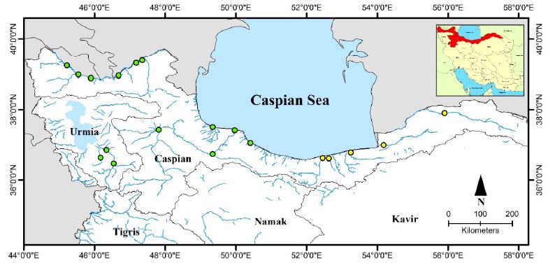
Figure 1: Distribution map of S. glanis in Iran; green circle: current distribution, yellow circle: previous distribution

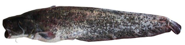
Figure 2: S. glanis, Recorded from Aras dam (Photo by: Jouladeh-Roudbar).

One of the most important habitats of Wels catfish in Iran is Aras Dam Lake in West Azerbaijan. In studies conducted on this river, Wels catfish have been caught from 6 selected stations in 3 stations along this river. There are also many hills above the dam lake, especially in the area called Cheshmeh Soraya, which is a border region between Iran, Turkey and Nakhchivan, where Wels catfish are concentrated. The river’s potential for the Wels catfish to live behind the Aras Dam has also been proven by scientists in the Republic of Azerbaijan. According to these studies, when the Nakhchivan water reservoir was built on the river in 1973, the predominant fish in the region were the Capoeta capoeta and Barbus cyri, but in 1976 the Wels catfish had the highest weight after the carp. The great depth of the reservoir along with its great length and width has been the cause of this growth.

Another Wels catfish habitat is the Manjil Dam Lake. The trout branches in Zanjan are also one of the places where there are many Wels catfish. The Atrak River in Golestan Province, the Tajan River in Sari, and the Bahnmir River on the outskirts of Babolsar are other Wels catfish habitats in Iran. Valiabad Tonekabon River, Amirkalayeh Wetland and most importantly Anzali Wetland are other places of life of this fish. The Fereydunkenar River was once the most important river in the life of the Wels catfish. In Azerbaijan, the Zarrinehrood, Siminehrood and Talkhehrud rivers (before the drought) were the habitats of the Wels catfish.

Reproduction

Fish usually reach sexual maturity in the second to fourth year of life, at which age the Wels catfish is about 60 to 70 cm long and weighs 900 to 2,000 grams. Wels catfish sometimes migrate up to 25 km for spawning. Wels catfish the male has a drooping skin at the end of the abdomen. In material, this part is smaller but thicker. Males are larger and have the task of caring for the egg and the baby. Wels catfish reproduces once a year. Reproduction takes place at a temperature of 18 to 20 degrees, which if this temperature is not provided, and reproduction will be delayed. Pairs play reproductive games before reproduction, including chasing and jumping out of water.

Wels catfish eggs are yellow and sticky, 3 mm in diameter, and attach to plants. Wels catfish nest. The relative uniformity is high and can reach up to 330,000 per kilogram, indicating that many eggs and larvae are killed. The absolute uniformity of small and medium-sized Wels catfish is from 480 to 11,000. The eggs are concentrated in clusters in the nest and the male fish, which has few sperm, fertilizes them and takes care of them until the larvae hatch (hatch). The incubation period of the eggs is 3 to 5 days (often 50 hours) at a temperature of 24 degrees Celsius. The larvae are about eight and a half millimeters long after hatching. The larvae do not leave the nest until they have absorbed the yolk sac. The eggs, and especially the Wels catfish larvae, like all larvae that live in the nest, have found special respiratory adaptations to withstand the lack of oxygen in the nest. Wels catfish grow very fast in the first year of life.

References

1. Jouladeh-Roudbar A, Eagderi S, Vatandoust S (2015) First record of Paraschistura alta (Nalbant and Bianco, 1998) from Eastern Iran and providing its COI barcode region sequences (Teleostei: Nemacheilidae). Iranian Journal of Ichthyology 2: 235-243.
2. Jouladeh-Roudbar A, Vatandoust S, Eagderi S, Jafari-Kenari S, Mousavi-Sabet H (2015) Freshwater fishes of Iran; an updated checklist. Aquaculture, Aquarium, Conservation & Legislation 8: 855-909.
3. Jouladeh-Roudbar A, Eagderi S, Esmaeili HR (2016a) First record of the striped bystranka, Alburnoides taeniatus (Kessler, 1874) from the Hari River basin, Iran (Teleostei: Cyprinidae). Journal of Entomology and Zoology studies 4: 788-791.
4. Jouladeh-Roudbar A, Eagderi S, Hosseinpour T (2016b) Oxynoemacheilus freyhofi, a new nemacheilid species (Teleostei, Nemacheilidae) from the Tigris basin, Iran. FishTaxa 1: 94-107.
5. Jouladeh-Roudbar A, Eagderi S, Soleimani A (2017a) First record of Petroleuciscus esfahani Coad and Bogutskaya, 2010 (Actinopterygii: Cyprinidae) from the Karun River drainage, Persian Gulf basin, Iran. International Journal of Aquatic Biology 4: 400-405.
6. Jouladeh-Roudbar A, Eagderi S, Ghanavi HR, Doadrio I (2017b) A new species of the genus Capoeta Valenciennes, 1842 from the Caspian Sea basin in Iran (Teleostei, Cyprinidae). ZooKeys 682: 137.
7. Jouladeh-Roudbar A, Eagderi S, Ghanavi HR, Doadrio I (2016c) Taxonomic review of the genus Capoeta Valenciennes, 1842 (Actinopterygii, Cyprinidae) from central Iran with the description of a new species. FishTaxa 1: 166-175.
8. Jouladeh-Roudbar A, Eagderi S, Murillo-Ramos L, Ghanavi HR, Doadrio I (2017c) Three new species of algae-scraping cyprinid from Tigris River drainage in Iran (Teleostei: Cyprinidae). FishTaxa 2: 134-155.
9. Jouladeh-Roudbar A, Eagderi S, Sayyadzadeh G, Esmaeili HR (2017d) Cobitis keyvani, a junior synonym of Cobitis faridpaki (Teleostei: Cobitidae). Zootaxa 4244: 118-126.
10. Jouladeh-Roudbar A, Ghanavi HR, Doadrio I (2020) Ichthyofauna from Iranian freshwater: Annotated checklist, diagnosis, taxonomy, distribution and conservation assessment. Zoological Studies 59: e21.
11. Vajargah MF, Namin JI, Mohsenpour R, Yalsuyi AM, Prokić MD, et al. (2021) Histological effects of sublethal concentrations of insecticide Lindane on intestinal tissue of grass carp (Ctenopharyngodon idella). Veterinary Research Communications 45: 373-380. [crossref]
12. Yalsuyi AM, Vajargah MF, Hajimoradloo A, Galangash MM, Prokić MD, et al. (2021) Evaluation of behavioral changes and tissue damages in common carp (Cyprinus carpio) after exposure to the herbicide glyphosate. Veterinary Sciences 8: 218. [crossref]
13. Vajargah MF, Mohsenpour R, Yalsuyi AM, Galangash MM, Faggio C (2021) Evaluation of histopathological effect of roach (Rutilus rutilus caspicus) in exposure to sub-lethal concentrations of Abamectin. Water, Air, & Soil Pollution 232: 1-8.
14. Vajargah MF (2021) A Review on the Effects of Heavy Metals on Aquatic Animals. ENVIRONMENTAL SCIENCES 2.
15. Vajargah MF, Yalsuyi AM, Hedayati A (2018) Effects of dietary Kemin multi-enzyme on survival rate of common carp (Cyprinus carpio) exposed to abamectin. Iranian Journal of Fisheries Sciences 17: 564-572.
16. Vajargah MF, Hedayati A (2017) Toxicity Effects of Cadmium in Grass Carp () and Big Head Carp (). Transylvanian Review of Systematical and Ecological Research 19: 43-48.
17. Yalsuyi AM, Hedayati A, Vajargah MF, Mousavi-Sabet H (2017) Examining the toxicity of cadmium chloride in common carp (Cyprinus carpio) and goldfish (Carassius auratus). Journal of Environmental Treatment Techniques 5: 83-86.
18. Vajargah MF (2022) Familiarity with Caspian Kutum (Rutilus kutum). Aquac Fish Stud 4: 1-2.
19. Sattari M, Imanpour Namin J, Bibak M, Forouhar Vajargah M, Bakhshalizadeh S, et al. (2020) Determination of trace element accumulation in gonads of Rutilus kutum (Kamensky, 1901) from the south Caspian Sea trace element contaminations in gonads. Proceedings of the National Academy of Sciences, India Section B: Biological Sciences 90: 777-784.
20. Sattari M, Bibak M, Bakhshalizadeh S, Forouhar Vajargah M (2020) Element accumulations in liver and kidney tissues of some bony fish species in the Southwest Caspian Sea. Journal of Cell and Molecular Research 12: 33-40.
21. Sattari M, Bibak M, Forouhar Vajargah M (2020) Evaluation of trace elements contaminations in muscles of Rutilus kutum (Pisces: Cyprinidae) from the Southern shores of the Caspian Sea. Environmental Health Engineering and Management Journal 7: 89-96.
22. Vajargah MF, Hossaini SA, Niazie EHN, Hedayati A, Vesaghi MJ (2013) Acute toxicity of two pesticides Diazinon and Deltamethrin on Tench (Tinca tinca) larvae and fingerling. International Journal of Aquatic Biology 1: 138-142.
23. Yousefi M, Jouladeh-Roudbar A, Kafash A (2020) Using endemic freshwater fishes as proxies of their ecosystems to identify high priority rivers for conservation under climate change. Ecological Indicators 112: 106137.

DOI: 10.31038/AFS.2022415

Abstract

An investigation was carried out at three selected stations in Salimpur sea beach in the Bay of Bengal, Chittagong, with special reference to abundance, composition, and a taxonomic group of zooplankton. Samples were collected from three stations these are ship-breaking yard, Salimpur mangrove forest area, fishery ghat Salimpur during monsoon (15/10/2019), and post-monsoon (15/01/2020). A total of 7 groups of zooplankton were identified. Copepods were the most important constituents of the zooplankton in all areas. Copepods accounted for 30.71%, 32.81%, 34.05% during monsoon and 25.75%, 25.96%, 27.31% during post-monsoon of the total zooplankton population. The other dominant constituents were Fish larvae (20.71%), Shrimp larvae (20.18%), Crab larvae (16.84%), sagitta (5.14%) which are the maximum of the total zooplankton population. The minimum density of Copepod is (55.89 ind/m³⁾ and the maximum density is (71.84ind/m³) recorded in January. During October this transverse into (65.64 ind/m³) in minimum and (101.94 ind/m³) in maximum. The high density of copepods shows a significant relationship between zooplankton and the environmental condition that work as an indicator of pollution.

Keywords

Zooplankton; Mangrove; Post-monsoon; Abundance; Biodiversity

Introduction

Zooplankton is microscopic animals that act as primary and secondary links in the food webs of all aquatic ecosystems. They feed on phytoplankton which directly provides a food source for larval vertebrates and invertebrates as well as related to the growth of juvenile and larger fish. Zooplankton is a marine microorganism with a swimming pool against major currents. Though limited in their ability to swim, they move day and night at intervals of hundreds of feet. They prefer to feed at night on the surface of the water and successfully feed on phytoplankton, which is why they are called living organisms. They tend to represent important interactions between the parasitic particles and large grazers [1]. In the tropics lead to fish production from human exploitation. Natural marine life is linked to the abundance of zooplankton and biodiversity. The viability of pelagic marine fish directly or indirectly depends on the discovery of zooplankton. In aquatic waters, zooplankton is used as an indicator of physiological, chemical, and biological processes due to its widespread distribution, small size, and rapid growth rates [2], high density, short life span, ecological diversity, of various types and tolerances of stress [3]. In food webs, organisms of the zooplankton represent a link from autochthonous material to higher trophic levels, e.g. juvenile riverine fish, which use backwaters as feeding grounds [4].

FAO’s survey report (1985) stated that Bangladesh’s tidal areas are rich in zooplankton. The abundance of zooplankton and its ecosystems in Bangladesh’s coast and harbors is rarely studied. [5] studied zooplankton in the northeastern part of the Bangladesh coast and found 18 genera and 18 species. [6] observed the macro-zooplankter of the continental shelf in the Bay of Bengal and reported on the occurrence and distribution of 18 calanoid copies. [7] recorded occasional variations of zooplankton in coastal waters in the southeastern part of Bangladesh. The major groups of zooplankton are copepods, Decapoda, Chaetognatha, cladocerans and fish, and shellfish. Zooplankton diversity of the saltwater area of the Bakkhali river, Cox’s Bazar, Bangladesh was also studied by [8]. The coastal area contains sensitive land and aquatic areas, such as mangrove forests, wetlands, and wet flats. On the shores of Sitakunda in the Chittagong region, the northeastern part of the Bay of Bengal is located near the Sandwip Chanel, which has wave particles, shipwrecks, and a community of fishermen and an important source of fishery resources. The purpose of this study is to provide more information on the quantity and structure of the zooplankton community in the coastal waters of Salimpur coast, north of the city of Chittagong, currently involved in coastal shipping operations.

As an important link in the conversion of energy from producers to consumers, free-living zooplanktonic organisms are a fundamental element of the aquatic environment. Organic zooplanktonic organisms are indicators of water quality bio due to their growth and distribution are closely related to natural boundaries. Zooplankton communities are often used as important tools to find changes in water quality and to assess the health of rural aquatic bodies.

The Zooplankton site is a group of different heterotrophic species that consume phytoplankton that stimulate nutrients through their metabolism and transfer energy to higher trophic levels (Deborah et al, 2010). Zooplanktons are playing a significant role in the ecosystem, as they are the second-largest food chain in the world. They play a key role in the transfer of power within their environment. They are found in the pelagic area of ​​lakes, lakes, rivers, and the sea where light enters. Zooplankton releases much organic matter, which dissolves and converts into the biomass of various bacteria. The zooplankton community is made up of major and second-largest consumers. They provide a direct link between early producers and high trophic levels as almost all fish depend on zooplankton for food during their caterpillar phase, while other fish continue to consume zooplankton throughout their lives (Madin et al. 2001).

The purpose of this study is to provide more information on the quantity and structure of the zooplankton community in the coastal waters of Salimpur coast, north of the city of Chittagong, currently involved in coastal shipping operations, to identify critical issues affecting the potential of zooplankton community structures, and to provide a monitoring tool to improve the water quality of water for future studies.

Objectives of the Study

1. To identify and get an account of the zooplankton community of the Salimpur coast.
2. To determine the abundance and distribution of zooplankton along with some Physico-chemical parameters of the study area.

The Study Area

Zooplankton collection and finding the quantity of zooplankton assigned to be 3 areas selected. The stations were a Salimpur ship-breaking yard, the Salimpur mangrove area, and the Salimpur fishery ghat area.

Station 1: Sampling station 1 is Salimpur ship breaking yard. It is a polluted area with heavy metal and oil pollution.

Station 2: This station is salimpur mangrove forest area, highly vegetation with biologically enhanced site.

Station 3: Sampling station 3 is fishery ghat of salimpur.

Geological position of three stations (Figure 1 and Table 1).

Figure 1: Study area

Table 1: GPS location of the study area

Station No.	GPS Coordinate
01.	22°21ʹ26ʺ N, 91°44ʹ59ʺ E
02.	22°22ʹ39ʺ N, 91°44ʹ45ʺ E
03.	22°23ʹ42ʺ N, 91°44ʹ28ʺ E

Methods and Materials

Sampling Period

1. In Post Monsoon (October 15)
2. In monsoon (January 15)

Investigation in Salimpur was carried out during Post Monsoon (October) and Monsoon (January) periods. Samples are collected from three selected stations. All samples were taken during high tide.

The sample was collected from three stations Salimpur sea beach. From post-monsoon October 15 2019 to winter 15 January 2020, two sampling data were collected. In this data collection, 3 stations were under data collection. All samples were taken during high tide. We have used mechanized boats to collect samples and to measure the other parameters of seawater like water temperature, water pH, water salinity, water transparency, DO.

Collection and Preservation of Zooplankton

Zooplankton sampling was carried out with the help of a conical zooplankton net made of Nylon Silk of 335-micrometer mesh size and having 12 cm circular mouth opening fitted with a plastic bucket at the cod. A digital flow meter was set up at the mouth of the net to record the amount of water filtered through the net during sampling. Samples were collected at the three sampling stations from the surface water for 10 to 15 min. After collecting samples were preserved in 5% formalin.

Staining and Sorting

For efficient sorting, the samples were stained with eosin and left for over the night. All the zooplankton attained reddish color rendering easy identification. The stained plankton was stored out from debris with a fine brush, needle, forceps and low power microscope was used during sorting. The sorted organisms were preserved in 70% ethanol.

Identification and Counting

The sorted organisms were brought under microscope and identified following [9-14] etc. In each catch, the total number of the individual count was done either by complete counting or by sub-sampling.

Interpretation of Data

The zooplankton concentration was calculated at individuals/m³. Where the total volume of water (m³) filtered through the net was calculated by using the following equation:

Total volume of water (m)={(FR-IR) × coefficient} × 2πr^2

Where,

FR=Final Reading

IR=Initial Reading

Co-efficient=0.3

π=3.1416

r=Radius of ring of used at plankton net=12 cm

The abundance of Zooplankton (individuals/m³)=Number of species in each group/volume of water.

Physiochemical Parameters

Sample Collection and Preservation

Water samples were taken from the surface with a bucket for the determination of different Physicochemical parameters. Data collection was collected by a different digital machine.

In situ Determination of Physicochemical Factor

Air and Water Temperature. Air and water temperature was measured by using a graduated centigrade thermometer.

Water Salinity. The water salinity was determined by using a Salinity Refractometer (tank new-100) and a digital salinity meter.

Hydrogen ion concentration of water (pH). For determining hydrogen ion concentration (pH), a digital pH meter was used.

Transparency. Water Transparency was determined by using a white Secchi disk of 30 cm diameter.

Determination of dissolved oxygen (DO). For determining dissolved oxygen (D.O), a digital DO meter was used.

Determination of TDS (mg/l). For determining Total Dissolved Solids (TDS), a digital TDS meter was used.

Determination of TSS (mg/l). At first, a filter paper was oven-dried for moisture-free at 60°C for 30 minutes. Then it will be kept into desiccators for cooling and then it will be weighted by an electric balance. Then a thoroughly mixed 100 ml samples will be filtered through the weighted filter paper. The filter paper will be allowed to dry completely and reweighted. The weight change will be multiplied by 10, thus total suspended solids (T.S.S) in 1L of water sample will be obtained.

Species Diversity Analysis

Zooplankton assemblage data were analyzed with the Plymouth Routines in Multivariate Ecological Research (PRIMER) statistical package version 6 (Clarke and Warwick, 06). Diversity of the species assemblage was analyzed by the Shannon-Wiener index (H’) [15-21], species richness was measured by Margalef index (d) and evenness was measured by Pielou’s index (J’) (Pielou, 1966). The value of the Shannon-Wiener index, Margalef index, and Pielou’s index calculated by the following formula:

Shannon-Wiener Diversity Index (H’)

H’=-∑ Pi × ln (Pi)

Where,

H’=Shannon-Wiener diversity index;

Pi=n/N; [n=No. Of individuals of species]

N=Total individuals;

Margalef Richness Index (d):

d=(s-1)/ln (n)

where,

S=Total species;

N=Total individuals;

Pielou’s Evenness Index (J’)

J’=H(s)/H(max)

Where,

H(s)=Shannon-Wiener information function

H(max)=The theoretical maximum value for H(s), if all species in the samples are equally abundant.

Result

Data Collection of Monsoon

Data Collection of Monsoon is shown in Figures 2-5 and Tables 2-9.

Figure 2: Abundance of zooplankton during Monsoon (Station-1)

Figure 3: Abundance of zooplankton in Monsoon ( Station-2)

Figure 4: Abundance of zooplankton in Station-3 during Monsoon

Figure 5: Comparison of species found in three stations during monsoon period

Table 2: Physiochemical parameters in Station- 1 during monsoon

Water temperature	22º c
Air temperature	25º c
Water transparency	6 cm
pH	7.9
Salinity	19 PPT
DO	2.48 mg/L
BOD	1.42  mg/L
TDS	21.88 g/L
TSS	276 mg/L
EC	33.68  ms/cm
PO4-P	0.64  ug/L
NO2-N	0.95  ug/L

Table 3: Species composition in station-1 during monsoon

Station- 01
Name of Species	Number of Individuals	Abundance (Ind/m3)	Percentage (%)
Copepod	109	55.89	30.71
Fish Larvae	65	33.30	18.29
Shrimp Larvae	47	24.10	13.24
Crab Larvae	67	34.36	18.88
Sagitta	19	9.74	5.35
Lucifer	25	12.82	7.04
Mysid	21	10.77	5.92
Unidentified	2	1.03	0.57
	=265	=182.01	=100%

Table 4: Physiochemical parameters in Station- 2 during monsoon

Water temperature	22 c
Air temperature	26 c
Water transparency	6 cm
pH	7.8
Salinity	21 PPT
DO	2.95 mg/L
BOD	1.2  mg/L
TDS	18.36 g/L
TSS	311 mg/L
EC	32.40  ms/cm
PO4-P	0.81 ug/L
NO2-N	1.12  ug/L

Table 5: Species composition in station- 2 during monsoon

Station- 02
Name of Species	Number of Individuals	Abundance (Ind/m3)	Percentage (%)
Copepod	148	71.84	32.81
Fish Larvae	79	38.35	17.52
Shrimp Larvae	53	25.73	11.61
Crab Larvae	73	35.44	16.19
Sagitta	26	12.62	5.76
Lucifer	36	17.48	7.98
Mysid	32	15.53	7.09
Unidentified	4	1.94	0.87
	=321	=218.93	=100%

Table 6: Physiochemical parameters at Station- 3 during monsoon

Water temperature	23  c
Air temperature	26 c
Water transparency	7 cm
pH	7.9
Salinity	22 PPT
DO	3.36 mg/L
BOD	1.18  mg/L
TDS	22.09 g/L
TSS	214 mg/L
EC	33.23  ms/cm
PO4-P	0.92 ug/L
NO2-N	1.45 ug/L

Table 7: Species composition in station- 3 during monsoon

Station- 03
Name of Species	Number of Individuals	Abundance (Ind/m^3)	Percentage (%)
Copepod	126	62.69	34.05
Fish Larvae	62	30.85	16.76
Shrimp Larvae	52	25.87	14.05
Crab Larvae	57	28.36	15.41
Sagitta	16	7.96	4.32
Lucifer	29	14.43	7.84
Mysid	26	12.94	7.03
Unidentified	2	0.99	0.54
	=370	=184.09	=100%

Table 8: Comparison of physiochemical parameters in three stations during monsoon

Parameters	Station 1	Station 2	Station 3
Water temperature	22º c	22 c	23  c
Air temperature	25º c	26 c	26 c
Water transparency	6 cm	6 cm	7 cm
pH	7.9	7.8	7.9
Salinity	19 PPT	21 PPT	22 PPT
DO	2.48 mg/L	2.95 mg/L	3.36 mg/L
BOD	1.42  mg/L	1.2  mg/L	1.18  mg/L
TDS	21.88 g/L	18.36 g/L	22.09 g/L
TSS	276 mg/L	311 mg/L	214 mg/L
EC	33.68  ms/cm	32.40  ms/cm	33.23  ms/cm
PO4P	0.64  ug/L	0.81 ug/L	0.92 ug/L
NO2N	0.95  ug/L	1.12  ug/L	1.45 ug/L

Table 9: Comparison of species found in three stations during monsoon period

Name of Species	Percentage			Average
	Station- 01	Station- 02	Station- 03
Copepod	30.71	32.81	34.05	32.52
Fish Larvae	18.29	17.52	16.76	17.52
Shrimp Larvae	13.24	11.61	14.05	12.96
Crab Larvae	18.88	16.19	15.41	16.83
Sagitta	5.35	5.76	4.32	5.14
Lucifer	7.04	7.98	7.84	7.62
Mysid	5.92	7.09	7.03	6.68
Unidentified	0.57	0.87	0.54	0.66

Data Collection of Post-Monsoon

Data Collection of Post-Monsoon is shown in Figures 6-10 and Tables 10-17.

Figure 6: Abundance of zooplankton in station-1 during post-monsoon

Figure 7: Abundance of zooplankton in Station-2 during post-monsoon

Figure 8: Abundance of zooplankton in station-3 during post-monsoon

Figure 9: Comparison of species found (%) in three stations during Post-monsoon

Figure 10: Abundance Variation of zooplankton between post-monsoon & monsoon

Table 10: Physiochemical parameters at Station-1 during post-monsoon

Water temperature	29º c
Air temperature	32º c
Water transparency	10 cm
pH	7.6
Salinity	14 PPT
DO	5.12 mg/L
BOD	2.90 mg/L
TDS	2.02 g/L
TSS	182 mg/L
EC	3.40 ms/cm
PO4-P	2.80 ug/L
NO2-N	2.58 ug/L

Table 11: Species found in station-1 during Post-monsoon

Station- 01
Name of Species	Number of Individuals	Abundance (Ind/m3)	Percentage (%)
Copepod	128	65.64	25.75
Fish Larvae	103	52.82	20.72
Shrimp Larvae	98	50.26	19.72
Crab Larvae	84	43.08	16.90
Sagitta	19	9.74	3.82
Lucifer	25	12.82	5.03
Mysid	38	19.49	7.65
Unidentified	2	1.03	0.40
	=497	=254.88	=100%

Table 12: Physiochemical parameters at Station-2 during post-monsoon

Water temperature	29 ºc
Air temperature	32º c
Water transparency	12 cm
pH	7.4
Salinity	14 PPT
DO	5.71 mg/L
BOD	2.50 mg/L
TDS	2.42 g/L
TSS	114 mg/L
EC	4.56 ms/cm
PO4-P	2.36 ug/L
NO2-N	2.58 ug/L

Table 13: Species found in station-2 during post-monsoon

Station- 02
Name of Species	Number of Individuals	Abundance (Ind/m3)	Percentage (%)
Copepod	210	101.94	25.96
Fish Larvae	169	82.04	20.89
Shrimp Larvae	153	74.27	18.91
Crab Larvae	141	68.45	17.43
Sagitta	45	21.84	5.56
Lucifer	36	17.48	4.45
Mysid	52	25.24	6.43
Unidentified	3	1.46	0.37
	=809	=392.72	=100%

Table 14: Physicochemical parameters in station-3 during post monsoon

Water temperature	31º c
Air temperature	33º c
Water transparency	13 cm
pH	7.4
Salinity	15 PPT
DO	5.88 mg/L
BOD	2.32 mg/L
TDS	2.88 g/L
TSS	110 mg/L
EC	4.99 ms/cm
PO4-P	2.18 ug/L
NO2-N	1.92 ug/L

Table 15: Species found in station-3 during post-monsoon

Station- 03
Name of Species	Number of Individuals	Abundance (Ind/m3)	Percentage (%)
Copepod	177	88.06	27.31
Fish Larvae	133	66.17	20.52
Shrimp Larvae	142	70.65	21.91
Crab Larvae	105	52.24	16.20
Sagitta	28	13.93	4.32
Lucifer	17	8.46	2.62
Mysid	44	21.89	6.79
Unidentified	2	0.99	0.31
	=648	=322.39	=100%

Table 16: Comparison of physiochemical parameter during Post-monsoon

Post Monsoon
Parameters	Station 1	Station 2	Station 3
Water temperature	29º c	29 ºc	31º c
Air temperature	32º c	32º c	33º c
Water transparency	10 cm	12 cm	13 cm
pH	7.6	7.4	7.4
Salinity	14 PPT	14 PPT	15 PPT
DO	5.12 mg/L	5.71 mg/L	5.88 mg/L
BOD	2.90 mg/L	2.50 mg/L	2.32 mg/L
TDS	2.02 g/L	2.42 g/L	2.88 g/L
TSS	182 mg/L	114 mg/L	110 mg/L
EC	3.40 ms/cm	4.56 ms/cm	4.99 ms/cm
PO4-P	2.80 ug/L	2.36 ug/L	2.18 ug/L
NO2-N	2.58 ug/L	2.58 ug/L	1.92 ug/L

Table 17: Comparison of species found in three stations during Post-monsoon

Name of Species	Percentage			Average
	Station-01	Station- 02	Station- 03
Copepod	25.75	25.96	27.31	26.34
Fish Larvae	20.72	20.89	20.52	20.71
Shrimp Larvae	19.72	18.91	21.91	20.18
Crab Larvae	16.90	17.43	16.20	16.84
Sagitta	3.82	5.56	4.32	4.56
Lucifer	5.03	4.45	2.62	4.03
Mysid	7.65	6.43	6.79	6.96
Unidentified	0.40	0.37	0.31	0.36

Biodiversity Index

Shannon-Wiener Diversity Index

H’=-∑ pi× ln (pi)

Where,

H’=Shannon-Wiener diversity index;

Pi=n/N; [n=No. Of individuals of species]

N=Total individuals;

Shannon-Wiener Diversity Index

Station	Post Monsoon	Monsoon
01	1.7900	1.7956
02	1.7930	1.8131
03	1.7996	1.7797

Margalef Richness index (d):

d=(s-1)/ln(n)

where:

S=Total species

N=Total individuals

Richness

Station	Post Monsoon	Monsoon
01	1.2885	1.3642
02	1.3441	1.6363
03	1.2357	1.3528

Pielou’s Evenness Index (J’)

J’=H(s)/H(max)

Where,

H(s)=Shannon-Wiener information function;

H(max)=The theoretical maximum value for H(s), if all species in the samples are equally abundant.

Evenness

Station	Post Monsoon	Monsoon
01	0.8147	0.8172
02	0.7787	0.7561
03	0.8190	0.8099

Discussion

Distribution and Abundance of Zooplankton

Zooplankton samples were sorted out into 7 major groups namely Copepod, Fish larvae, shrimp larvae, Crab larvae, Sagitta, Lucifer, mysid.

Total number of zooplankton varied from 182.01 Ind/m³ to 392.72 Ind/m³ in studied are throughout the research period.

Copepods

The number of Copepods during monsoon was recorded 34.05 % as the highest percentage. The lowest amount was found in post monsoon which is 26. 34%. The abundance density was found 55.89 ind/m³, 71.84 ind/m³, 62.69 ind/m³ in monsoon and 65.64 ind/m³, 101.94 ind/m³, 88.06 ind/m³ in post monsoon.

Fish Larvae

From the recorded data, we saw that the percentage of fish larvae in post monsoon is higher than the percentage in monsoon. It is 20.71 % and 17.52 %. The abundance density in post monsoon was 52.82 ind/m³, 82.04 ind/ m³ and 66.17 ind/ m³. And 33.30 ind/ m³, 38.35 ind/ m³, 30.85 ind/ m³ in monsoon.

Shrimp Larvae

In monsoon, the amount of shrimp larvae was 12.96% and in post monsoon it increased to 20.18%. It was a little bit lower in monsoon than in post monsoon.

Crab Larvae

The percentages of crab larvae during post monsoon were 16.90% 17.43% 16.20%and in monsoon were 18.88%, 16.19%, 15.41%. That is the average is almost close in post monsoon and monsoon.

Sagitta

The amount of Sagitta in post monsoon was recorded 5.14% and in monsoon it was 4.56 %.That is in monsoon it was a little bit more than post monsoon. The abundance density was found 9.74 ind/ m³, 21.84 ind/ m³, 13.93 ind/ m³ in post monsoon and 9.74 ind/ m³, 12.62 ind/ m³, 7.96 ind/ m³ in monsoon.

Lucifer

From the recorded information, in monsoon it was quite a large amount of Lucifer then In post monsoon. 7.62 % in monsoon and 4.03% in post monsoon.

Mysid

Both in monsoon and post monsoon, percentages were almost the same. In monsoon it was 6.88 % and in post monsoon it was 6.96%. The abundance density was 19.49 ind/ m³ , 25.24 ind/ m³ and 21.89 ind/ m³ in post monsoon. And in monsoon it was 10.77 ind/ m³, 15.53 ind/ m³ and 12.94 ind/ m³ .

Shannon Diversity

In Shannon diversity index(H¢) the highest value was recorded 1.8131 at station-2 during Monsoon, and the lowest value was recorded 1.7797 at station-3 during monsoon. . As the value was higher in station-2 it is well diverse than others station.

In post-monsoon the highest value was recorded 1.7996 at station-3 and lowest value was 1.7900 at station-1. As the value was higher in station-3 it is well diverse than others station.

Pielou¢s Evenness Index

The evenness (J¢) was ranges between 0.7561 to 0.8172 during monsoon and 0.7787 to 0.8190 during post monsoon in the study area.

The highest value was found in Station 3 during post monsoon.

Margalef Richness Index

The richness (d) was found in a range of 1.35 to 1.63 at monsoon and 1.23 to 1.34 during post monsoon.

The highest value was found in Station 02 during monsoon.

Hydrological Parameters

Temperature

Water temperature is very important for aquatic organism. In the monsoon season the water temp was around 29-31°C and the air temperature was around 31-33°C. In winter season the water temperature was recorded 22-24°C and the air temperature was around 24-26°C.

PH

PH is one of the major factor for aquatic environment .The highest value was found 7.9 and lowest was recorded 7.4.

Water Transparency

The highest transparency of water was highest recorded 13 cm and lowest was 6 cm.

Dissolved Oxygen

In post monsoon season the dissolved oxygen (DO) was recorded 5.12-5.88 ml/L and in the monsoon 2.48-3.36 mg/L.

Salinity

In the post monsoon season the salinity was recorded around 14-16 PPT and in the monsoon season the salinity was recorded around 19-23 PPT.

BOD

In post monsoon season the Biological oxygen demand (BOD) was recorded 2.32-2.90 mg/L and In monsoon the Biological oxygen demand (BOD) was recorded 1.18-1.42 mg/L.

TDS

In post monsoon season the total dissolved solid (TDS) was recorded 2.02-2.88 mg/L and in monsoon, total dissolved solid was recorded 19.88-22.23 mg/L.

TSS

In post monsoon season total suspended solids (TSS) was recorded 110-182 mg/L and in monsoon season total suspended solids was recorded 214-311 mg/L.

Limitation of the Study

Currently in the current study on the inequality of sampling and disruption therefore due to the covid-19 pandemic condition. Further study is needed for a concrete conclusion

Conclusion

There are some differences between the three stations. The abundance of zooplankton is higher in station-02 which is mangrove forest area coast, Salimpur. Abundance is high here because of suitable parameters & nutrients, and it is a less polluted station than others. From the research, it is clear that the abundance in station-03 is a bit low and station-01 is the lowest. Station-03 is a fishery ghat and station 01 is a ship breaking yard. Such an environment is risky for the abundance of zooplankton.

Acknowledgement

I would like to thank our honourable director Dr, Md. Shafiqul Islam who gave me this opportunity to do this research and our lab technician for helping us at the time of lab analysis and all whom helped us in this research.

References

1. Laval-Peuto Michèle, John F Heinbokel, Roger Anderson O, Fereidoun Rassoulzadegan, Barry Sherr F (1986) Role of Micro- and Nanozooplankton in Marine Food Webs. International Journal of Tropical Insect Science 7: 387-395.
2. Heinbokel JF (1978) Studies on the Functional Role of Tintinnids in the Southern California Bight. I. Grazing and Growth Rates in Laboratory Cultures. Marine Biology 53: 23-32.
3. Gajbhiye SN (2002) Zooplankton Study Methods,Importance and Significant Observations. Proceedings of the National Seminar on Creeks, Estuaries and Mangroves – Pollution and Conservation 21-27.
4. Kurmayer R, Keckeis H, Schrutka S, Zweimueller I (1996) Macro- and microhabitat used by 0+ fish in a side-arm of the River Danube Arch. Hyrobiol Suppl 113: 425-432.
5. Islam AKMN, Aziz A (1975) A preliminary study on zooplankton of the North-eastern Bay of Bengal. Bangladesh journal of Zoology 3: 125-138.
6. Bhuiyan AL, Mohis A, Das NG (1982) Macro zooplanktons of the continental shelf of The Bay of Bengal. Ctg. Uni. Studies, part (ii) 651: 59.
7. Ali A, Shukanta S, Mahmood N (1985) Seasonal abundance of plankton in Moheshkhali channel, Bay of Bengal. In proceedings of SAARC seminar on Protection of Environment from Degradation, Dhaka, Bangladesh 128- 140.
8. Ali M (2006) Zooplankton diversity of salt marsh habitat in the Bakkhali river estuary, Cox’s Bazar, Bangladesh. 4th year project paper, Institute of Marine Sciences and Fisheries (IMSF), University of Chittagong, 56.
9. Zafar M (1986) Study on the zooplankton of Shatkhira estuarine system in the vicinity of aquaculture farms with special reference to penaiedpost larvae. M.Sc. thesis, Institute of Marine Sciences and Fisheries, University of Chittagong 238.
10. Smith SV, Hollibaugh JT (1993) Coastal Metabolism and the Oceanic Organic Carbon Balance. Reviews of Geophysics 31: 75-89.
11. Afrin R (2006) Study on diurnal and tidal variation of zooplankton in the eastern coast of Saint Martin’s Island. Research paper, Institute of Marine Sciences and Fisheries, University of Chittagong 6.
12. Kurmayer R, Keckeis H, Schrutka S, Zweimueller I (1996) Macro- and microhabitat used by 0+ fish in a side-arm of the River Danube Arch. Hyrobiol Suppl 113: 425-432.
13. Madaputra M, Nair SRR, Achuthankutty CT, Nai VR (1981) Zooplankton abundance of around the Andaman-Nicoberisland. J. Mar. SC 17: 75-77.
14. Sikder SC (1976) Taxonomy of cyclopoid copepods of the Karnaphuli river estuary. M.Sc. 45 Project (unpublished), Institute of Marine Sciences and Fisheries, University of Chittagong 22.
15. Zafar M (2000) Study on Sergestid shrimp Acetes in the vicinity of Matamuhuri river confluence, Bangladesh. PhD. Thesis, (2000), University of Chittagong, Studies Sci 13: 115-122.
16. Das S (1977) Taxonomy of calanoid copepods of Karnaphuli river estuary. M.Sc. project (unpublished), Institute of Marine Sciences and Fisheries, University of Chittagong 22.
17. Goswami SC, Devassy VP (1991) Seasonal fluctuation in the occurrence of cladocera in the Madorizuari estuarine waters of Goa. J. Mar. Sci 20: 138-142.
18. Mustafa S, Nair VR, Govinda V (1999) Zooplankton community of Bhayander and Thane saltplans around Bombay. Indian J. Mar. Sci. 28: 184-191.
19. Khan MSK, Uddin SA, Haque MA (2015) Abundance and composition of zooplankton at Shitakundo coast in Chittagong, Bangladesh. Agric. Livest. Fish 2: 151-160.
20. Mahmood N, Khan YSA (1980) On the occurrence of post larvae and juvenile Penaeid shrimp at Bakkhali river estuary. Final report of UGC research, Dhaka, Bangladesh 26.
21. Khair SA, Bhuiyan AL, Das NG (1979) Distribution of Schmackeria lobipes of the Karnaphuli river estuary. M.Sc. thesis (unpublished), Institute of Marine Sciences and Fisheries, University of Chittagong 82.

DOI: 10.31038/AFS.2022414

Abstract

Caspian roach, Rutilus caspicus must have adaptive mechanisms to control internal homeostasis over a broad range of ambient various such as the heat shock (HS) and salinity changes. This experiment was carried out in two stages. In first stage, thirty juveniles fish (3.2 ± 0.34 g) transferred to 20 L circular tanks, containing three different salinity (5, 10, 15 ppt). Initially, half of the treatments exposed to a HS (26°C for 2 h) while the range of normal temperature was 16.5-17.5°C. At 96 h after transferring, survival rate, hematocrit, plasma Na⁺, K⁺ and Cl^– and osmolality and gill NKA activity were determined. In the second stage (second 96 h), all of the first treatments were transferred to 15 ppt and similar sampling was done. In first stage, no mortality in 5 and 10 ppt of both non heat shock (NHS) and HS treatments and higher plasma osmolality, ions (except K⁺), and hematocrit were observed. Mortality was observed in 15 ppt of NHS and in second stage, both treatments of 15 ppt showed mortality (15-20%). In NHS, significant increase of gill NKA found at in 10 ppt of second stage while in HS treatment was in 10 ppt of first stage. Changes in plasma osmolality and electrolytes in HS treatment were more less similar to NHS treatment. Together, it seems HS and salinity changes resulted to disturbances from an internal fluid shift thus a stress situation and Caspian roach juveniles need to complete ion-osmo regulation systems for adaptation with brackish water.

Keywords

Heat shock, Salinity, Osmoregulation, Gills, Na⁺/K⁺-ATPase activity

Introduction

In teleost fishes, highly efficient ion/osmoregulatory mechanisms lead to maintenance of body fluid homeostasis, which is necessary for the normal operation of cellular biochemical/physiological processes [1]. Approximately 5% of teleost fish are euryhaline while the most teleost fish are stenohaline and cannot tolerate large changes in salinity [2,3]. Euryhaline teleosts have the ability to adapt to different environmental salinities while maintaining essentially constant their internal milieu by the activation of several osmoregulatory mechanisms, namely in the branchial and renal epithelia [4,5]. Gills, kidney and digestive tract are the main osmoregulatory organs in teleost fishes [4,6]. The rapid response and/or acute transition to changing environmental salinity become a crucial challenge for avoiding significant internal osmotic disturbances. There are two periods of acclimation for euryhaline teleosts to hyperosmotic environments: a) a crisis period (minutes to hours) involving a rapid increase in gill-ion fluxes, activating exist proteins, water transport and/or other mechanisms [7], and elevated plasma ions and osmolality followed by b) a regulatory period (hours to days onward) including increases of gill Na⁺/K⁺-ATPase (NKA) activity accompanied by a proliferation and development of mitochondrion-rich cells (MRCs) presumably hormonally regulated allowing for increased transport capacity [8], increasing net Na⁺ and Cl^– efflux and restoring plasma ions balance [9,10]. Na⁺/K⁺-ATPase, primary driving force for flux of intra and extra cellular NaCl which is specifically present in high concentrations on the basolateral side of MRCs, plays important roles in maintaining the cell membrane potential by pumping Na⁺ out and K⁺ in through active transport [9]. Changes in gill NKA activity are observed 2-3 days after transfer from a hypoosmotic to hyperosmotic environment in euryhaline teleosts [11]. In anadromous species [12,13], activation of gill NKA takes place 3-7 days after transfer to SW and also in mullet and killifish, gill NKA activity elevated rapidly within 3 h after transfer from FW to BW or SW [14]. In both of FW and seawater (SW), the regulation of the ion levels and osmolality of body fluids of fishes are doing actively [2]. The plasma osmolalities of euryhaline teleost species of FW and SW origin vary [15] and in a number of euryhaline teleosts showed the effects of changing salinity on plasma osmolality and circulating electrolytes [16-21].

Since the most organisms on Earth are ectotherms, such as fish, surviving and adaptation to temperature fluctuations are crucial for them (Somero, 2010; Tang et al., 2014). Rapid water temperature changes (exceeds the optimal temperature range) or exposures to sustained temperatures outside the optimal range (thus, sub-optimal) often result in thermal stresses or lethal conditions (Portz et al., 2006). The fishes can be classified into two groups including eurythermal and stenothermal species which tolerance wide and narrow ranges of temperature, respectively [22,23]. Internal electrolyte and osmotic homeostasis in aquatic ectotherms can be influenced by environmental temperature [17,24,25] which is contributed to the regulation of ion-transporting mechanisms by many proteins while stenothermal species have marginally stable of cellular proteins in a limited range of temperature [17,24,26].

The Caspian roach, Rutilus caspicus (Yakovlev 1870) belongs to the Cyprinidae, the largest family among FW teleosts, is moderately euryhaline, omnivorous feeding on small crustacea and insect larvae and often lives in areas close to the estuary where water is brackish. Spring and fall migrations, from sea to the river and sea inner migration for spawning and wintering, occur in its life, respectively [27] and also considered as a significant food source for beluga sturgeon, Huso huso (L. 1758) in the Caspian Sea [10,28]. This species has been considered for inclusion in the list of threatened species for the region due to over fishing and deterioration of its spawning ground [29]. Since reproduction and sustainability of teleosts species stocks such as Caspian roach negatively are affected due to the human activities in the southern of Caspian Sea, moreover the critical importance of reconstruction such resources, fisheries organization in Iran, using artificial propagation program for releasing millions of different kinds of teleosts larva and juveniles, derived through artificial propagation, to connected rivers to the Caspian sea [10]. Being a eurythermal fish, Caspian roach like cyprinus carpio L. must have adaptive mechanisms to control internal homeostasis over a broad range of ambient temperatures particularly in releasing time (May-July) while the fish exposing to the heat shock and salinity changes in transferring processes.

The main goals of the present study were to determine the effects of short-term elevation temperature and direct salinity transferring stresses on the osmoregulatory capability of Caspian roach. Considering the value of gill NKA response it is worth to study of the impact of to environmental stresses such as temperature and salinity on osmoregulatory responses in Caspian roach. The selected salinity treatments were base of the salinity range that Caspian roach are likely to encounter in Bandare Torkaman coastal area, Gorgan bay, southeastern of the Caspian Sea, Iran.

Material and Methods

Animals

Approximately 600 juvenile (aged between 3 and 4 months) Caspian Roach, were obtained from the Sijual Teleost Fish Propagation and Rearing Center, close to the Bandare Torkaman, southeast of the Caspian Sea, Iran. The fish were transferred to Aquaculture research center of the Faculty of Fisheries and Environmental Sciences, Gorgan University of Agricultural Sciences and Natural Resources, Gorgan, Iran. All fish were acclimatized to laboratory conditions for at least two weeks prior to experiments in six 400 l fiberglass tanks, with approximately 150 juveniles in each tank, to avoid the potentially confounding effects of handling stress (e.g. high blood cortisol) on osmoregulation [30]. Fish were fed twice daily with a commercial diet, biomar (0.8; Nersac, France) during holding. Fish were not fed during the experiment. Fish were exposed to ambient photoperiod of approximately 14 h light:10 h dark.

Dechlorinated tap water was used during the experiment and Caspian seawater (SW) with maximum salinity of 15 ppt (obtained from Bandare Torkaman sea shore, Gorgan Bay, Iran) were used for preparing waters of different salinities, ppt. Salinity, temperature (range 16.5-17.5°C), pH (range 8.2-8.6) and dissolved O₂ (7.6-13.3 mg l⁻¹) were measured daily to the nearest 0.1‰, 0.1°C, 0.1 pH unit, 0.1 mg l^–1, respectively using a water quality meter (U-10, Horiba Ltd, Japan).

Salinity Acclimation Experiment

The experiment was carried out in two stages including three salinity treatments with three replicates. Feeding was stopped 24 hour before starvation. After adaptation with experimental conditions, initially, half of the treatments exposed to the heat shock (HS), 26°C for 2 hours (h), while the range of normal temperature was 16.5-17.5°C. In first stage, thirty juveniles fish (3.20 ± 0.34 g) directly transferred to the 20 L volume plastic circular tanks, containing three different salinity (5, 10 and 15 ppt). At 96 h after transferring, survival rate, haematocrit, Na⁺, K⁺, Cl^–and osmolality concentrations and gill NKA activity were determined.

In the second phase, all of the first phase individuals were transferred to 15 ppt. At second 96 h after transferring, similar sampling mentioned above were performed. Twelve individuals were sampled two times, just before transferring to other salinities (second phase). About 24 individuals, per treatment groups, of this specie were used for the experiment.

Sampling

The six fish from each treatment were anesthetized with clove powder (100 mg/l) and samples of the blood were taken immediately into a 75 mm heparinised capillary tubes by caudal transaction. Capillary tubes with blood samples were centrifuged at 5000g (Hettich: D_78532 Tuttlingen, Germany) for 15 min at 4°C, for the measurement of haematocrit (Hct) and aliquots of plasma were stored at -80°C [10].

Analytical Techniques

Plasma Ion and Osmolality Measurements

Plasma Na⁺, K⁺ and Cl^– concentrations were measured using an ion-selective electrodes (Electrolit analyzer mod EI-99IE, Germany) and results reported in mEq·l⁻¹. Plasma osmolality was determined in fresh samples using a freezing point depression (OSMOMETER AUTOMATIC model. Roebling, Germany) and reported as mOsmo1. l⁻¹ [10].

Gill Na⁺/K⁺-ATPase Activity

Gill NKA activity was measured according to the McCormick (1993) microassay protocol with some modifications [10,31]. Gill filament samples from the leftside second arch were served by fine point scissors, from the anesthetized fish and immersed in 100 μl of ice-cold SEI buffer (150 mmol.l^–1 sucrose, 10 mmol.l^–1 EDTA, 50 mmol.l^–1 imidazole, pH 7.3) and frozen at -80°C.

The thawed filaments were homogenized with pestle in SEI buffer containing 0.1% deoxycholic acid and centrifuged at 8000g for 60 s to remove large debris. For the assay 25 μl of the supernatant were added to 500 μl of assay mixture (Imidazole buffer (50 mM) Phosphoenolpyruvate (2.8 mM), NADH (0.22 mM), ATP (0.7 mM), Lactic Dehydrogenase (4.0 U), Pyruvate Kinase (5.0 U). Assays were run in two sets of duplicates, one set containing the assay mixture and the other assay mixture plus ouabain (1.0 mM; Sigma-Aldrich Chemical Co., St. Louis, MO, USA) to specifically inhibit NKA activity. ATPase activity was detected by enzymatic coupling of ATP dephosphorylation to NADH oxidation measured at 340 nm with a spectrophotometer (Photometer clinic Π, Iran) for 10 min at 30°C. Total protein concentrations were determined by modification of the Bradford (1976) dye binding assay with a bovine serum albumin (BSA) standard at 630 nm and the results expressed as mmoles ADP/mg protein/hour.

Statistical Analysis

All the data are expressed as means with standard deviation (SD). Analysis the data of plasma ions, osmolality and gill NKA activity between groups was carried out using one-way analysis of variance (ANOVA) by SPSS (17) in individuals. Statistically significant differences were expressed as p < 0.05.

Ethical Statement

The collection and use of experimental animals in this study complied with Iranian animal welfare laws, guidelines and policies, and was approved by the Gorgan University of Agricultural Sciences and Natural resources, College of Fisheries and Environment, Gorgan, Iran and the Portuguese Animal Welfare Law (Decreto-Lei no.197/96) and animal protocols were approved by CIIMAR/UP.

Results

Survival

No mortality occurred in 5 and 10 ppt of non-heat shock (NHS) treatments in first stage (Figure 1). However, after 96 h exposure mortality was significantly higher in 15 ppt of NHS treatments in first stage (Figure 1). There were a non-significant mortality in 5 and 10 ppt of heat shock (HS) treatments in first stage (Figure 1). In the second stage, a significant mortality was observed in 10 ppt of HS treatment and 15 ppt of both NHS and HS treatments (Figure 1).

Figure 1: Mortality percentage of R. caspicus in the first (96 h) and second stages (192 h), dotted bars, of salinity acclimation in 5, 10 and 15 ppt with (HS) and non-heat shock (NHS). Values are means + s.d. (n = 6). Bars with the same lower case letters are not significantly different from each other (P < 0·05).

Osmoregulatory Indicators: Plasma Ions and Osmolality

Blood parameters from stages 1 and 2 are presented in Figures 2 and 3, respectively. Plasma Na⁺ and Cl⁻ levels increased significantly in most of treatments compared with control in first and second stages (Figures 2a, 2b, 3a and 3b) except Cl⁻ levels in 5 and 10 ppt of fist stages (Figure 2b). Plasma K⁺ levels were not altered by 96 h acclimation (first stage) to 5, 10 or 15 ppt (Figure 2c) however were significantly lower following second stage except in 5 ppt of HS treatment (Figure 3c). Plasma osmolality showed an significant increase only in 15 ppt of NHS at first stage (Figure 2d) however all of treatment in the second stage showed significant increase (Figure 3d).

Blood haematocrit showed significant increase in in 5 and 15 ppt of NHS while there was not significant change at HS treatment at first stage (Figure 2e). The all treatments in second stage showed significant increase compare to control group (Figure 3e).

Gill NKA Activity

Na⁺/K⁺-ATPase activity in gill was rather similar to the initial levels in the FW control treatment after 96 exposures in 5, 10 or 15 ppt and only HS treatment at 10 ppt showed significant increase in first stage (Figure 2f). At the second stage (192 h), only 10 ppt of NHS showed a significant increase in gill NKA activity compared with the control group (Figure 3f). In NHS treatment, 5 and 10 ppt showed higher NKA activity rather than 15 ppt while in HS treatment NKA activity of individuals at 15 ppt was higher than 5 ppt (Figure 3f). In each salinity, NKA activity of 5 and 10 ppt at NHS were higher than HS treatments while it was inverse at 15 ppt (Figure 3f).

Figure 2: Plasma (a) sodium, (b) chloride and (c) potassium concentrations (mEq·l^-1), (d) osmolality (mosmo.kg⁻¹) and (e) haematocrit (%) as well as (f) gill Na⁺/K⁺-ATPase activity (mmoles ADP/mg protein/hour) of  R. caspicus transferred from 0  to 5, 10 and 15ppt  and acclimated for 96h at each salinity, first stage. Dotted bars represent heat shock (HS) treatment. Values are means ± S.E.M. (n=6 whole times). Bars with the same lower case letters are not significantly different from each other (P<0.05).

Figure 3: Plasma (a) sodium, (b) chloride and (c) potassium concentrations (mEq·l^-1), and (d) osmolality (mosmo.kg⁻¹) and (e) haematocrit (%) as well as (f) gill Na⁺/K⁺-ATPase activity (mmoles ADP/mg protein/hour) of  R. caspicus transferred from first stage ( 0  to 5, 10 and 15ppt) to second stage (15 ppt) and acclimated for second 96h (192h) at given salinity (5, 10 and 15ppt). Dotted bars represent heat shock (HS) treatment. Values are means ± S.E.M. (n=6 whole times). Bars with the same lower case letters are not significantly different from each other (P<0.05).

Discussion

Acclimated R. caspicus to higher salinity had higher plasma osmolality and ions (except K⁺), and hematocrit. Salinity of 5 and 10 ppt represents the more natural salinity range of Caspian roach. However, acclimation to 15 ppt has allowed us to test the osmoregulatory abilities of R. caspius under more challenging conditions. In the first stage, the direct transfer to 5 and 10 ppt in both NHS and HS treatments resulted to no mortality which might indicate relative ability of Caspian roach to tolerate such environmental condition changes. However, the observed mortality in 15 ppt of NHS and/or HS treatment might express imposed stress due to synergism effect of stressors. In NHS, two times increase in gill NKA found in 10 ppt after transferring from first to second stage which might be contributed to rather intermediate salinity at first stage then increase positively with salinity at the second stage. In HS treatment, detected higher gill NKA at 10 ppt at first stage might be related to the stress of HS and requiring stabilizing the energy consuming then reduced to the half in second stage as regulatory period. Changes in plasma osmolality and electrolytes in HS treatment were more less similar to NHS treatment which might be occurring of initial dehydration. However, it seems that HS and salinity changes have some physiological effects on ion regulation in this fish. Together, these data representing disturbances from an internal fluid shift potentially due to water loss and elevated plasma osmolality which may be problematic resulting in a stress situation and mortality.

Survival

The observation of no mortality duration of direct transfer to 5 and 10 ppt in both NHS and HS treatments at the first stage, indicating relative ability of this fish to tolerate such salinity changes. [32] expressed the metabolic cost of osmoregulation is reduced in brackish water (BW), because the blood-medium osmotic gradient is minimal. In contrast, gradual transfer of Caspian roach to different salinities (5, 10 or 15 ppt) resulted no mortality [10]. The goldfish Carassius auratus (L. 1758) showed high survival under chronic exposure to salinities of 5 and 10 ppt while significant mortality was observed at salinities of 15 and 20 ppt [33]. Such observation might be related to different level of endocrine and ionoregulatory pathways developing, as has been suggested in some works [34] on smoltification in salmonids or due to social hierarchies, which can also influence ionoregulatory capacity [35] and also change in chloride cells morphology and restoration of homeostasis [36,37]. The direct transferring of Common carp, Cyprinus carpio (L.). to environmental salinity (2.5, 5, and 7.5‰) showed a great adaptation and higher survival rate [38]. [39] reported survival rates of lake trout (S. namaycush), brook trout (S. fontinalis) and Atlantic salmon (Salmo salar) were 80%, 50% and 100%, respectively following direct transferring to 30 ppt. [40] reported direct transfer of FW-adapted white sturgeon juveniles from FW to 16 ppt was associated with 25 to 30% mortality, indicating that these fish have some ability to tolerate large changes in salinity for up to 5 days. [32] reported Nile tilapia, Oreochromis niloticus, which were transferred directly to full strength SW (36 ppt) for 14 days whole mortality occurred in this period. However, O. mossambicus and its hybrids showed not survive by direct transfer to salinities of 35 psu [25,41]. The observed mortalities in 15 ppt of NHS treatments might be related to osmotic shock of direct transfer to this salinity and also delay in gill NKA activation in response to osmotic challenge that is proposed to reflect changing gene expression but also transcript expression and protein synthesis [42-45]. In second stage, both treatments of 15 ppt showed mortality (15-20%) which might be indicted to imposed stress because of HS and subsequent apoptosis [46] and also osmotic challenge of transferring to this salinity on the other word synergism effect of stressors.

Osmoregulatory Indicators: Plasma Ions and Osmolality

Salinity challenges typically alter plasma osmolality and electrolytes levels in euryhaline teleosts with an initial crisis stage followed by a regulatory stage [7,10,11,12,20]. The observed plasma ion concentrations were in the range of other teleost fish species [47]; see reviews by [48]. The elevated plasma osmolality, and electrolytes (except plasma K⁺) of Caspian roach in the most treatments of both stages might be contributed to the occurring of initial dehydration due to osmotic efflux of water from the fish by osmosis and diffusional ion influx of electrolytes from the environment [39,45,49]. Blood osmolality in teleost fish is 280-360 mmol kg⁻¹, and is tightly regulated in a species-dependent range of salinities [15]. In present study based on comparison to euryhaline fish, the values of Na⁺, Cl^– and osmolality are relatively high suggesting that the fish have relatively poor salinity tolerance, or that they are in a temporary state of ion imbalance. Also increased levels of electrolytes concentrations had not returned to initial concentration (control treatment) as has been reported in [50]. The rather similar results observed in gradual transferring of Caspian roach to different salinity levels (5, 10 or 15 ppt) [10].

In general changes in hematology can be explained by changes in ionoregulatory status [40] and it is one of the secondary stress responses in fish [51,52]. Hematocrit showed a positive correlation with salinity in both stages, as has been reported by (Platichthy flesus: [53]; Gymnocypris przewalskii: [10,20,54,55] and in most anadromous teleosts studied to date (Oncorhynchus mykis: [56]; O. tshawytscha: [57]; S. salar: [58]) or sturgeon (Acipenser oxyrinchus, A. brevirostrum: Baker et al., 2005). By attention to previous finding which indicating to the important role of effective hormones such as cortisol, prolactin, in acclimation phase to osmotic and environmental challenges (several hours to several days after stress) [8], this result might be interpreted by measuring hormonal changes but not done in the present study thus measuring hormones which are involving in response to environmental challenges could be helpful in future study.

Gill Na⁺/K⁺-ATPase Activity

The assessment of osmoregulatory status/ability of teleosts has been achieved by using the branchial NKA activity responses (mRNA and protein expression) [1,59]. The alterations in gill NKA activity in relation to environmental salinity are diverse, but two typical situations seem to prevail: (i) a direct relationship, characteristic of anadromous species, in which higher salinities induce higher values of NKA activity [60] and (ii) a U-shaped relationship, described for some euryhaline teleosts, in which lower values of NKA activity occur at intermediate salinities and higher values at low and high salinities [10,11,45,61-63]. There are various reports which express/state no effect of salinity on NKA activity (Gillichthys mirabilis: [64]), conversely, strong effect of medium salinity on gill NKA activity (Scophthalmus maximus: [65]), positive correlation between environmental salinity and NKA activity (Oreochromis mossambicus: [66]; Onchorhynchus keta: [67]) and negative correlation (F. heteroclitus: [68]; O. mossambicus: [20,69]). Short- and long term acclimation to environmental salinity have examined intermediate metabolism changes in euryhaline fishes [70-74]. Gaumet et al. (1995) suggested that NKA activity is generally lowest in fish living in a medium whose salinity is equivalent to that of the blood. An ecologically theory would state that fish would be adapted to spend the least amount of osmoregulatory energy in environmental salinities they evolved to live in. Also, physiologically we would expect the energy consuming NKA activity to be minimal at environmental salinities isosmotic to blood [10,75]. According our results most changes occurred in 10 ppt of NHS treatments (Figure 2f). The observed two times increase in gill NKA of 10 ppt after transferring from the first to second stage (15 ppt) might be contributed to rather intermediate salinity at first stage then increase positively with salinity at second stage. Adaptation of Caspian roach individuals to different salinity presumably can be results increasing the number of entering ions to the body thus occurring water loss by osmosis. In continue, increasing/or tendency to increase in gill NKA activity occurring to absorb water from the external environment [21] however, decreased significantly at the salinity of 15 ppt. The latter might be due to the increase of plasma Na⁺ and Cl^– as the major electrolytes in the body fluid and their critical role in osmoregulation [59] which result to increase plasma osmolality under higher salinity condition thus decrease of NKA activity. The similar results have been reported in the juvenile largemouth bass adapted to saline waters [21] and Mozambique tilapia [76]. In juvenile turbot (Scophthalmus maximus) reduced gill NKA activity at 15‰ salinity levels would lead to reduced energy expenditures [65]. In another experiment, gill NKA activity of Caspian roach decreased with salinity in the short term with activity being the lowest in fish kept 48 h at 15 ppt although with longer acclimation (+96h) returned to control levels [10]. Furthermore, the results of this study might be indicating that Caspian roach are a bit intolerant of salinity. Some studies revealed that the source of changing NKA activity upon salinity challenge might be alterations on mRNA level [43,77], or protein level (O. mossambicus: [78,79], or both levels [80]; O. mossambicus: [69]). In general, related to the effect of abrupt transfer to different salinities on physiologic /osmoregulatory functions more studies are required. Perhaps, Caspian roach like salmonids, anadromous species, [45] activation of gill NKA takes place 3-7 days after transfer to higher salinity or that 15 ppt is just not enough salinity to induce increases. It would be of interest to see if the fish can survive long term exposure (2 weeks or more) to 15 ppt (or more) and what the levels of plasma ions and gill NKA activity are after this acclimation.

Heat Shock (HS)

The ambient temperature can effect on the internal ionic and osmotic balance of fish [17,24,81,82]. Rapid temperature changes, heat or cold shocks, are among the stressors with a high physiological impact on fish [83,84]. Changes in plasma osmolality and electrolytes in HS treatment were more less similar to NHS treatment which might be occurring of initial dehydration. A reduction was observed in plasma K⁺ level accompanied by salinity increase in the second stage. It has been shown that in SW the fish gills are permeable to K⁺ that efflux is greater than influx [85]. This would indicate that reduced uptake, rather than increased loss of K⁺, is the more important factor contributing to the poor performance of fish [10,86]. Also, change in gill NKA activity [45] and passive efflux of K⁺ from kidney segments [87] can be potential reasons for such reduction. After exposure of R. caspicus to short term increasing temperature condition, ascending trend in first stage and significant increase of plasma osmolality at second stage were found (Figure 2d and 3d). Even though the gill NKA was not affected (Figure 2f). Moreover, NKA activity was assayed at the higher level than exposure temperature of the fish that might show the apparent NKA activity not provide a physiological interpretation of our results. The protein conformation, kinetic properties, and assembly can be affected by influencing of temperature on the reactivity of molecules [88]. The activation of ion transporter system is energy-required while the main process for energy providing, the rate of cellular respiration, is temperature-dependent [89]. Therefore, detected higher gill NKA at 10 ppt at first stage might be related to the stress of HS and requiring stabilizing the energy consuming then reduced to the half in second stage as regulatory period (Figure 2f) which potentially reflected that metabolically-dependency of ion transporter proteins to temperature change rather susceptible to passive ion diffusion [89-92]. Furthermore, inhabitation of specific activity of NKA by temperature was found in the Mozambique tilapia and common carp [88]. It was found that a lower apparent NKA activity was compensated by strongly enhanced NKA expression [17,24]. The present study was difficult to rule out the possibility of heat shock having much of an impact on overall ion regulation although clear responses to salinity can be found. Study on the heat shock proteins (HSP70, 90) by suing immunoblotting and gene expression (PCR-qPCR) considering response to the environmental stress such as heat shock or salinity changes, measurement the plasma cortisol, lactate and glucose might be interest for future works.

Conclusion

It seems that Caspian roach juveniles need to complete ion-osmo regulation systems for adaptation with BW and biochemistry-physiologic parameters of juveniles are determinant their adjustment to the natural conditions. According the management point of view, it seems that HS and salinity changes have some physiological effects concern ion regulation in this fish. Although for more confidence, study various salinities, different time of sampling and other environmental tolerances such as temperature, culture density, diet and also focus on the expression patterns of ion transporters such as NKA, Na⁺/K⁺/2Cl⁻ (NKCC), cystic fibrosis transmembrane conductance regulator (CFTR, chloride channel), V-ATPase proton pump in the gills, kidney and digestive tract [24,55] are needed.

Acknowledgments

The study was supported by the University of Gorgan. We are very grateful to Mrs. Yalda Sheikh for assistance in preparation of solutions. We would also like to thank Dr. Stephen McCormick and Dr. Vahid Khori for their advises and comments. We would like to thank anonymous referees for comments on an earlier version of the manuscript.

References

1. Hwang PP, Lee TH (2007) New insights into fish ion regulation and mitochondrion-rich cells. Comparative Biochemistry and Physiology – Part A: Molecular & Integrative Physiology 148: 479-497. [crossref]
2. Edwards SL, Marshall WS (2012) Principles and patterns of osmoregulation and euryhalinity in fishes,” in SC McCormick, AP Farrell, CJ Brauner (eds.) Fish Physiology-Euryhaline Fishes (London: Academic Press) 32: 1-44.
3. Hiroi J, Yasumasu S, McCormick SD, Hwang PP, Kaneko T (2008) Evidence for an apical Na-Cl cotransporter involved in ion uptake in a teleost fish. Journal of Experimental Biology 211: 2584-2599. [crossref]
4. Marshall WS, Grosell M (2006) Ion transport, osmoregulation and acid-base balance,” in (Eds.), DH Evans and JB Claiborne. The Physiology of Fishes (Boca Raton, FL: CRC Press), 177-230.
5. Schultz ET, McCormick SD (2013) Euryhalinity in an evolutionary context. In SD McCormick, AP Farrell, CJ Brauner (EDs.). Fish Physiol. 32. Academic Press, pp. 477-533.
6. Takei Y, Hwang PP (2016) Homeostatic Responses to Osmotic Stress. In: CB Schreck, L Tort, AP Farrell, CJ Brauner (Eds.) Fish Physiology-Biology of stress in fish. 35 Academic Press Inc San Diego, United States Elsevier 208-237.
7. Wang PJ, Lin CH, Hwang LY, Huang CL, Lee TH, et al. (2009) Differential responses in gills of euryhaline tilapia, Oreochromis mossambicus, to various hyperosmotic shocks. Comparative Biochemistry and Physiology – Part A: Molecular & Integrative Physiology 152: 544-551. [crossref]
8. McCormick SD, Bradshaw D (2006) Hormonal control of salt and water balance in vertebrates. General Comparative Endocrinology 147: 3-8. [crossref]
9. Evans DH, Piermarini PM, Choe KP (2005) The multifunctional fish gill: dominant site of gas exchange, osmoregulation, acid–base regulation, and excretion of nitrogenous waste. Physiological Review 85: 97-177. [crossref]
10. Malakpour Kolbadinezhad S, Hajimoradloo A, Ghorbani R, Joshaghani H, Wilsonm JM (2012) Effects of gradual salinity increase on osmoregulation in Caspian roach Rutilus caspicus. Journal of Fish Biology 81: 125-134. [crossref]
11. Jensen MK, Madsen SS, Kristiannsen K (1998) Osmoregulation and salinity effects on the expression and activity of Na+/K+-ATPase in gills of European sea bass (Dicentrachus labrax) L. Journal of Experimental Zoology 282: 290-300.
12. Madsen SS, Naamansen ET (1989) Plasma ionic regulation and gill Na+/K+–ATPase changes during rapid transfer to sea water of yearling rainbow trout (Salmo gairdneri): time course and seasonal variation. Journal of Fish Biology 34: 829-840.
13. Berge AI, Berg A, Fyhn HJ, Barnung T, Hansen T, et al. (1995) Development of salinity tolerance in underyearling smolts of Atlantic salmon (Salmo salar) reared under different photoperiods. Canadian Journal of Fisheries and Aquatic Sciences 52: 243-251.
14. Mancera JM, McCormick SD (2000) Rapid activation of gill Na+/K+-ATPase in the euryhaline teleost (Fundulus heteroclitus). Journal of Experimental Zoology 287: 263-274. [crossref]
15. Varsamos S, Wendelaar Bonga SE, Charmantier G, Flik G (2004) Drinking and Na+/K+-ATPase activity during early development of European sea bass (Dicentrarchus labrax): ontogeny and short–term regulation following acute salinity changes. Journal of Experimental Marine Biology and Ecology 311: 189-200.
16. Kang CK, Tsai SC, Lee TH, Hwang PP (2008) Differential expression of branchial Na+/K+-ATPase of two medaka species, Oryzias latipes and Oryzias dancena, with different salinity tolerances acclimated to fresh water, brackish water and seawater. Comparative Biochemistry and Physiology 151: 566-575.
17. Sardella BA, Kültz D, Cech J Jr, Brauner C (2008a) Salinity-dependent changes in Na+/K+-ATPase content of mitochondria-rich cells contribute to differences in thermal tolerance of Mozambique tilapia. Journal of Comparative Physiology 178: 249-256.
18. Christensen AK, Hiroi J, Schultz ET, McCormick SD (2012) Branchial ionocyte organization and ion-transport protein expression in juvenile alewives acclimated to freshwater or seawater. Journal of Experimental Biology 215: 642-652. [crossref]
19. Tait JC, Mercer Evan W, Gerber L, Robertson GN, Marshall WS (2017) Osmotic versus adrenergic control of ion transport by ionocytes of Fundulus heteroclitus in the cold. Comp Biochem Physiol A Mol Integr Physiol 203: 255-261. [crossref]
20. Malakpour Kolbadinezhad S, Coimbra J, Wilson JM (2018a) Osmoregulation in the Plotosidae catfish: role of the salt secreting dendritic organ. Frontiers in Physiology 9: 761.
21. Yi H, Chen X, Liu S, Han L, Liang J, et al. (2021) Growth, osmoregulatory and hypothalamic–pituitary–somatotropic (HPS) axis response of the juvenile largemouth bass (Micropterus salmoides), reared under different salinities Aquaculture Reports 20.
22. Somero GN (2010) The physiology of climate change: how potentials for acclimatization and genetic adaptation will determine ‘winners’ and ‘losers’. Journal of Experimental Biology 213: 912-920.
23. Long Y, Li L, Li Q, He X, Cui Z (2012) Transcriptomic characterization of temperature stress responses in larval zebrafish. PLoS ONE 7: 37209. [crossref]
24. Metz JR, van der Burg EH, Wendelaar-Bonga SE, Flik G (2003) Regulation of branchial Na+/K+-ATPase in common carp Cyprinus carpio acclimated to different temperatures. Journal of Experimental Biology 206: 2273-2280. [crossref]
25. Sardella BA, Matey V, Cooper J, Gonzalez RJ, Brauner CJ (2004) Physiological, biochemical and morphological indicators of osmoregulatory stress in `California Mozambique tilapia (Oreochromis mossambicus x O. urolepis hornorum) exposed to hypersaline water. Journal of Experimental Biology 207: 1399-1413. [crossref]
26. Crockett EL, Londraville RL (2006) Temperature, in: Evans DH, Claiborne JB (Eds.), The Physiology of Fishes, Marine Biology Series. CRC, Taylor & Francis, Boca Raton, 497 FL 231-269.
27. Sattari M (2002) Ichtiology (1), Anatomy and Physiology. Gilan University Publication. 378p (in Persian).
28. Keyvanshokooh S, Ghasemi A, Shahriari-Moghadam M, Nazari RM, Rahimpour M (2007) Genetic analysis of Rutilus rutilus caspicus (Jakowlew 1870) populations in Iran by microsatellite markers. Aquaculture Research 38: 953-956.
29. Kiabi BH, Abdoli A, Naderi M (1999) Status of the fish fauna in the South Caspian basin of Iran. Zoology in the Middle East 18: 57-65.
30. Biswas AK, Seoka M, Takii K, Maita M, Kumai K (2006) Stress response of red sea bream (Pagrus major) to acute handling and chronic photoperiod manipulation. Aquaculture 252: 566-572.
31. Wilson JM, Leitão A, Gonçalves AF, Ferreira C, Reis-Santos P (2007) Modulation of branchial ion transporter protein expression by salinity in glass eels Anguilla anguilla L. Marine Biology 151: 1633-1645.
32. Guner Y, Ozden O, Cagiran H, Altunko M, Kizak V (2005) Effect of salinity on the osmoregulation function of the gill in Nile tilapia (Orechormic niluticus). J. Vet. Anim. Sci 29: 1259-1266.
33. Schofield PJ, Brown ME, Fuller PL (2006) Salinity tolerance of goldfish, Carassius auratus, a non-native fish in the United States. JSTOR 69: 258-268.
34. Beckman BR, Larsen DA, Dickhoff WW (2003) Life history plasticity in Chinook salmon: relation of size and growth rate to autumnal smolting. Aquaculture 222: 149-165.
35. Sloman KA, Scott GR, Diao Z, Rouleau C, Wood CM, et al. (2003a) Cadmium affects the social behaviour of rainbow trout (Oncorhynchus mykiss). Aquatic Toxicology 65: 171-185. [crossref]
36. Kelly SP, Woo NYS (1999) The response of sea bream following abrupt hypoosmotic exposure. Journal of Fish Biology 55: 732-750.
37. Ouattara N, Bodinier C, Negre-Sadargues G, D’Cotta H, Messad S, et al. (2009) Changes in gill ionocyte morphology and function following transfer from fresh to hypersaline waters in the tilapia Sarotherodon melanotheron. Aquauculture 290: 155-164.
38. Saravanan M, Ramesh M, Petkam R, Poopal RK (2018) Influence of environmental salinity and cortisol pretreatment on gill Na+/K+ -ATPase activity and survival and growth rates in Cyprinus carpio. Aquaculture Reports 11: 1-7.
39. Hiroi J, McCormick SD (2007) Variation in salinity tolerance, gill Na+/K+-ATPase, Na+/K+/2Cl–cotransporter and mitochondria–rich cell distribution in three salmonids (Salvelinus namaycush, Salvelinus fontinalis and Salmo salar). Journal of Experimental Biology 210: 1015-1024. [crossref]
40. Mojazi Amiri B, Baker DW, Morgan JD, Brauner CJ (2009) Size dependent early salinity tolerance in two sizes of juvenile white sturgeon (Acipenser transmontanus). Aquaculture 286: 121-126.
41. Hwang P, Sun CM, Wu SM (1989) Changes of plasma osmolarity, chloride concentration and gill Na+/K+-ATPase activity in tilapia (Oreochromis mossambicus) during seawater acclimation. Marine Biology 100: 295-299.
42. Lee TH, Hwang PP, Shieh YE, Lin CH (2000) The relationship between ‘‘deep-hole’’ mitochondria-rich cells and salinity adaptation in the euryhaline teleost (Oreochromis mossambicus). Fish Physiology and Biochemistry 23: 133-140.
43. Seidelin M, Madsen SS, Blenstrup H, Tipsmark CK (2000) Time-course changes in the expression of Na+/K+-ATPase in gills and pyloric caeca of brown trout (Salmo trutta) during acclimation to seawater. Physiological and Biochemical Zoology 73: 446-453. [crossref]
44. Tipsmar CK, Madsen SS, Seidelin M, Christensen AS, Cutler CP, et al. (2002) Dynamics of Na+‏/K+‏/2Cl- cotransporter and Na+/K+-ATPase expression in the branchial epithelium of brown trout (Salmo trutta) and Atlantic salmon (Salmo salar). Journal of Experimental Zoology 293: 106-118.
45. Laiz–Carrión R, Guerreiro PM, Fuentes J, Canario AVM, Martín del Río MP, et al. (2005) Branchial osmoregulatory response to salinity in the gilthead sea bream (Sparus auratus). Journal of Experimental Zoology 303: 563-576. [crossref]
46. DuBeau SF, Pan F, Tremblay GC, Bradley TM (1998) Thermal shock of salmon in vivo induces the heat shock protein (Hsp70) and confers protection against osmotic shock. Aquaculture 168: 311-323.
47. Whittamore JM (2012) Osmoregulation and epithelial water transport: lessons from the intestine of marine teleost fish. Journal of Comparative Physiology B 182: 1-39.
48. Freire CA, Prodocimo V (2007) Special challenges to teleost fish osmoregulation inenvironmentally extreme or unstable habitats. in: B Baldisserotto, JM Mancera, BG Kapoor (Eds.), Fish Osmoregulation. Science Publishers, Enfield, 249-276.
49. Fielder DS, Allan GL, Pepperalla D, Parkhurst PM (2007) The effect of changes in salinity on osmoregulation and chloride cell morphology of juvenile Australian snapper (Pagrus auratus). Aquaculture 272: 656-666.
50. Martinez-Alvarez RM, Sanz A, Garcia-Gallego M, Domezain A, Domezain J, et al. (2005) Adaptive branchial mechanisms in the sturgeon (Acipenser naccarii) during acclimation to saltwater. Comp Biochem Physiol A Mol Integr Physiol 141: 183-190. [crossref]
51. Portz DE, Woodley CM, Cech Jr JJ (2006) Stress-associated impacts of short-term holding on fishes. Reviews in Fish Biology and Fisheries 16: 125-170.
52. Sopinka NM, Donaldson MR, O’Connor CM, Suski CD, Cooke SJ (2016) Stress Indicators in Fish. In: CB Schreck, L Tort, AP Farrell, CJ Brauner (Eds.) Fish Physiology – Biology of stress in fish. 35 Academic Press Inc San Diego, United States Elsevier. pp: 405-462.
53. Jensen FB, Lecklin T, Busk M, Bury NR, Wilson R, et al. (2002) Physiological impact of salinity increase at organism and red blood cell levels in European flounder (Platichthy flesus). Journal of Experimental Marine Biology and Ecology 274: 159-174.
54. Wang YS, Gonzalez RJ, Patrick ML, Grosell M, Zhang C, et al. (2003) Unusual Physioliology of scale-less carp (Gymnocypris przewalskii) in lake Qinghai: a high altitude alkaline saline lake. Comparative Biochemistry and Physiology A 134: 409-421.
55. Malakpour Kolbadinezhad S, Coimbra J, Wilson JM (2018b) Effect of dendritic organ ligation on striped eel catfish Plotosus lineatus osmoregulation. PLoS One 13: e0206206. [crossref]
56. Wang Y, Heigenhauser GJF, Wood CM (1994) Integrated responses to exhaustive exercise and recovery in rainbow trout white muscle: acid–base, phosphogen, carbohydrate, lipid, ammonia, fluid volume and electrolyte metabolism. Journal of Experimental Biology 195: 227-258.
57. Gallaugher PE, Thorarensen H, Kiessling A, Farrell AP (2001) Effects of high intensity training on cardiovascular function, oxygen uptake, internal oxygen transport and osmotic balance in Chinook salmon (Oncorhynchus tshawytscha) during critical speed swimming. Journal of Experimental Biology 204: 2861-2872. [crossref]
58. Kieffer JD, Rossiter AM, Kieffer CA, Davidson K, Tufts BL (2002) Physiology and survival of Atlantic salmon following exhaustive exercise in hard and softer water: implications for the catch-and -release sport fishery. North American Journal of Fisheries Management 22: 132-144.
59. Kaneko T, Watanabe S, Lee KM (2008) Functional morphology of mitochondrion-rich cells in euryhaline and stenohaline teleosts. Aquatic Bioscience Monographs (ABSM) 1: 1-62.
60. McCormick SD (1995) Hormonal control of gill Na+/K+-ATPase and chloride cell function. In: CM Wood, TJ Shuttlewoth, (Eds.), Fish Physiology 14. San Diego, CA: Academic Press. Pp. 285-315.
61. Lisboa V, Barcarolli IF, Sampaio LA, Bianchini A (2015) Effect of salinity on survival, growth and biochemical parameters in juvenile Lebranch mullet Mugil liza (Perciformes: Mugilidae). Neotropical Ichthyology 13: 447-452.
62. Zhang YT, Huang S, Qiu HT, Li Z, Mao Y, et al. (2017) Optimal salinity for rearing Chinese black sleeper (Bostrychus sinensis) fry. Aquaculture 476: 37-43.
63. Liu B, Guo HY, Zhu K, Guo L, Liu B, et al. (2019) Growth, physiological, and molecular responses of golden pompano Trachinotus ovatus (Linnaeus, 1758) reared at different salinities. Fish Physiology and Biochemistry 45: 1879-1893. [crossref]
64. Yoshikawa JSM, McCormick SD, Young G, Bern HA (1993) Effects of salinity on chloride cells and Na+/K+-ATPase activity in the teleost (Gillichthys mirabilis). Comp Biochem Physiol Comp Physiol 105: 311-317. [crossref]
65. Imsland AK, Gunnarsson S, Foss A, Stefansson SO (2003) Gill Na+/K+-ATPase activity, plasma chloride and osmolality in juvenile turbot (Scophthalmus maximus) reared at different temperatures and salinities. Aquaculture 218: 671-683.
66. Kültz D, Bastrop R, Jürss K, Siebers D (1992) Mitochondria–rich (MR) cells and the activities of the Na+/K+-ATPase and carbonic anhydrase in the gill and opercular epithelium of (Oreochromis mossambicus) adapted to various salinities. Comparative Biochemistry and Physiology 102: 293-301.
67. Uchida K, Kaneko T, Yamauchi K, Ogasawara T, Hirano T (1997) Reduced hypoosmoregulatory ability and alteration in gill chloride cell distribution in mature chum salmon (Onchorhynchus keta) migrating upstream for spawning. Marine Biology 129: 247-253.
68. Marshall WS, Emberley TR, Singer TD, Bryson SE, McCormick SD (1999) Time course of salinity adaptation in a strongly euryhaline estuarine teleost (Fundulus heteroclitus): a multivariable approach. Journal of Experimental Biology 202: 1535-1544. [crossref]
69. Lin CH, Huang CL, Yang CH, Lee TH, Hwang PP (2004) Time–course changes in the expression of Na+/K+-ATPase and the morphometry of mitochondrion–rich cells in gills of euryhaline tilapia (Oreochromis mossambicus) during freshwater acclimation. Journal of Experimental Zoology 301: 85-96. [crossref]
70. Sangiao-Alvarellos S, Laiz-Carrion R, Guzman JM, Martın del Rio MP, Mancera JM, et al. (2003) Acclimation of Sparus aurata to various salinities alters energy metabolism of osmoregulatory and nonosmoregulatory organs. American Journal of Physiology 285: 897-907. [crossref]
71. Sangiao-Alvarellos S, Arjona FJ, Martín del Río MP, Míguez JM, Mancera JM, et al. (2005). Time course of osmoregulatory and metabolic changes during osmotic acclimation in Sparus auratus. Journal of Experimental Biology 208: 4291-4304. [crossref]
72. Arjona FJ, Vargas-Chacoff L, Ruiz-Jarabo I, Martin del Rio MP, Mancera JM (2007) Osmoregulatory response of Senegalase sole (Solea senegalensis, Kaup 1858) to changes in auratus L., a non-native fish in the United States. Florida Scientist 69: 258-268.
73. Herrera M, Vargas-Chacoff L, Hachero I, Ruı´z-Jarabo I, Rodiles A, et al. (2009) Osmoregulatory changes in wedge sole (Dicologoglossa cuneata, Moreau 1881) after acclimation to different environmental salinities. Aquaculture Research 40: 762-771.
74. Vargas-Chacoff L, Arjona FJ, Polakof S, Martin del Rio MP, Soengas JL, et al. (2009) Interactive effects of environmental salinity and temperature on metabolic responses of gilthead sea bream Sparus aurata. Comparative Biochemistry and Physiology A Mol Integr Physiol 154: 417-424. [crossref]
75. Saoud IP, Kreydiyyeh S, Chalfoun A, Fakih M (2007) Influence of salinity on survival, growth, plasma osmolality and gill Na+/K+-ATPase activity in the rabbit fish (Siganus rivalatus). Journal of Experimental Marine Biology and Ecology 348: 183-190.
76. Vonck APMA, Wendelaar Bonga SE, Flik G (1998) Sodium and calcium balance in Mozambique tilapia, Oreochromis mossambicus, raised at different salinities. Comp Biochem Physiol A Mol Integr Physiol 119: 441-449. [crossref]
77. Scott GR, Richards JG, Forbush B, Isenring P, Schulte PM (2004) Changes in gene expression in gills of the euryhaline killifish (Fundulus heteroclitus) after abrupt salinity transfer. American Journal of Physiology 287: 300-309. [crossref]
78. Lee TH, Feng SH, Lin CH, Hwang YH, Huang CL, et al. (2003) Ambient salinity modulates the expression of sodium pumps in branchial mitochondria–rich cells of Mozambique tilapia (Oreochromis mossambicus). Zoological Science 20: 29-36. [crossref]
79. Lin YM, Chen CN, Lee TH (2003) The expression of gill Na+/K+-ATPase in milkfish (Chanos chanos) acclimated to seawater, brackish water and fresh water. Comparative Biochemistry and Physiology A Mol Integr Physiol 135: 489-497. [crossref]
80. D’Cotta H, Valotaire C, Le Gac F, Prunet P (2000) Synthesis of gill Na+/K+-ATPase in Atlantic salmon smolts: differences in a-mRNA and a-protein levels. American Journal of Physiology 278: 101-110. [crossref]
81. Fiess JC, Kunkel-Patterson A, Mathias L, Riley LG, Yancey PH, et al. (2007) Effects of environmental salinity and temperature on osmoregulatory ability, organic osmolytes, and plasma hormone profiles in the Mozambique tilapia (Oreochromis mossambicus). Comparative Biochemistry and Physiology – Part A: Molecular & Integrative Physiology 146: 252-264. [crossref]
82. Sardella BA, Sanmarti E, Kültz D (2008b) The acute temperature tolerance of green sturgeon (Acipenser medirostris) and the effect of environmental salinity. Journal of Experimental Zoology. A. Ecol genet Physiol 309: 477-483. [crossref]
83. Crawshaw LI (1979) Responses to rapid temperature change in vertebrate ectotherms. Ameriacn Zoology 19: 225-237.
84. Tanck MWT, Booms GHR, Eding EH, Bonga SEW, Komen J (2000) Cold shocks: a stressor for common carp. Journal of Fish Biology. 57: 881-894.
85. Sanders MJ, Kirschner LB (1983) Potassium metabolism in seawater teleosts II. Evidence for active potassium transport extrusion across the gill. Journal of Experimental Biology 104: 29-40.
86. Partridge GJ, Lymbery AJ (2008) The effect of salinity on the requirement for potassium by barramundi, Lates calcarifer, in saline groundwater. Aquaculture 278: 164-170.
87. Schwarzbaum PJ, Wieser W, Niederstatter H (1991) Contrasting effects of temperature acclimation on mechanisms of ionic regulation in a eurythermic and a stenothermic species of freshwater fish (Rutilus rutilus) and (Salvelinus alpinus). Comparative Biochemistry and Physiology 98: 483-489.
88. Tang CH, Leu MY, Shao K, Hwang LY, Chang WB (2014) Short-term effects of thermal stress on the responses of branchial protein quality control and osmoregulation in a reef-associated fish, Chromis viridis. Zoological Studies 53: 21.
89. Hochachka PW, Somero GN (2002) Biochemical adaptation: mechanism and process in physiological evolution 480. Oxford University Press, New York.
90. Schreck CB, Tort L (2016) The Concept of Stress in Fish. In Fish Physiology – Biology of In: CB Schreck, L Tort, AP Farrell, CJ Brauner (Eds.) Fish Physiology-Biology of stress in fish. 35 Academic Press Inc San Diego, United States Elsevier. pp. 1-34.
91. Martínez-Montaño E, Pontigo JP, Yáñez A, Ruiz-Jarabo I, Mancera JM, et al. (2015) Effects on the metabolism, growth, digestive capacity and osmoregulation of juvenile of Sub-Antarctic Notothenioid fish Eleginops maclovinus acclimated at different salinities. Fish Physiol Biochem 41: 1369-1381. [crossref]
92. Wang PJ, Lin CH, Hwang HH, Lee TH (2008) Branchial FXYD protein expression in response to salinity change and its interaction with Na+/K+-ATPase of the euryhaline teleost Tetraodon nigroviridis. Journal of Experimental Biology 211: 3750-3758. [crossref]

References

1. Johns Hopkins University Coronavirus Resource Center, https://coronavirus.jhu.edu/.
2. Deliso Meredith (2021) “Arizona ‘hottest hot spot’ for COVID-19 as health officials warn of hospital strain: The state has the highest infections per capita globally, based on JHU data, ABC News. 2021. https://abcnews.go.com/US/arizona-hottest-hot-spot-covid-19-health-officials/story?id=75062175.
3. Chow Denise, Joe Murphy (2021) These three states have the worst Covid infection rates of anywhere in the world: Arizona currently has the highest per capita rate of new Covid-19 infections, with 785 cases per 100,000 people over the past seven days, followed closely by California and Rhode Island, NBC News. https://www.nbcnews.com/science/science-news/these-three-states-have-worst-covid-infection-rates-anywhere-world-n1252861.
4. Britannica, Arizona state, United States, https://www.britannica.com/place/Arizona-state.
5. My Life Elsewhere, Arizona is around the same size as Italy.
6. https://www.mylifeelsewhere.com/country-size-comparison/arizona-usa/italy.
7. United States Census Bureau, Quick Facts, https://www.census.gov/quickfacts/AZ.
8. Eng H (2020) Arizona and COVID-19. Medical & Clinical Research 5: 175-178.
9. Eng H (2021) Arizona Reopening Phase 2: Rise and Fall of COVID-19 Cases. Medical & Clinical Research 6: 114-118.
10. Eng H (2021) Arizona Reopening Phase 3 and COVID-19: Returning to Normal. Medical & Clinical Research 6: 687-669.
11. White House Proclamation on Declaring a National Emergency Concerning the Novel Coronavirus Disease (COVID-19) Outbreak. 2020.
12. https://www.whitehouse.gov/presidential-actions/proclamation-declaring-national-emergency-concerning-novel-coronavirus-disease-covid-19-outbreak/.
fig 1
Teens Evaluating Tag Lines of Foods: The Relevance of Seemingly ‘Throw Away’ Messages Revealed by Mind Genomics Cartography
DOI: 10.31038/NRFSJ.2022513
Abstract
In a large-scale study of teen food cravings using Mind Genomics, respondents evaluated short vignettes comprising 2-4 messages each, created by combining 36 elements about food. The source elements fell into, four silos of nine elements each (food, situation, taglines for emotions, brand/benefits). Silo C, taglines, was previously thought to be irrelevant to respondents who paid attention primarily to the descriptions of the food and the eating experience. Reanalysis of the data at the level of the individual respondent, and focusing only on the taglines for the products, revealed a rich source of information about how respondents feel about products, how males differ from females, how self-rated hunger drives different pattern of responses to the taglines, and uncovered three new-to-the-world mind-sets. The results suggest that taglines, often assumed to be ‘throw aways’ in test concepts, can actually provide a measure of the way the respondent feels about the food, this measure obtained in a subtle, almost projective fashion, with the focus on the internals of the person, not on the externals of describing the food and the eating.
1. Pilgrim FJ, Peryam DR (1958) Sensory testing methods: A manual (No. 25-58). ASTM International.
2. Harvey K, Kemps E, Tiggemann M (2005) The nature of imagery processes underlying food cravings. British Journal of Health Psychology 10: 49-56. [Crossref]
3. Tiggemann M, Kemps E (2005) The phenomenology of food cravings: the role of mental imagery. Appetite 45: 305-313. [Crossref]
4. Weingarten HP, Elston D (1991) Food cravings in a college population. Appetite 17: 167-175. [Crossref]
5. Gofman A, Moskowitz H (2010) Isomorphic permuted experimental designs and their application in conjoint analysis. Journal of Sensory Studies 25: 127-145.
6. Moskowitz H, Silcher M, Beckley J, Minkus-McKenna D, Mascuch T (2005) Sensory benefits, emotions and usage patterns for olives: using Internet-based conjoint analysis and segmentation to understand patterns of response. Food Quality and Preference 16: 369-382.
7. Moskowitz H, Itty B, Ewald J (2003) Teens on the Internet-Commercial application of a deconstructive analysis of ‘teen zine’ features. Journal of Consumer Behaviour: An International Research Review 3: 296-310.
8. Foley M, Beckley J, Ashman H, Moskowitz HR (2009) The mind-set of teens towards food communications revealed by conjoint measurement and multi-food databases. Appetite 52: 554-560. [Crossref]
9. Moskowitz HR, Gofman A, Beckley J, Ashman H (2006) Founding a new science: Mind Genomics. Journal of Sensory Studies21: 266-307.
10. Biró B, Gere A (2021) Purchasing bakery goods during COVID-19: A Mind Genomics cartography of Hungarian consumers. Agronomy 11: 1645.
11. Moskowitz H, Beckley J, Adams J (2002) What makes people crave fast foods?. Nutrition Today37: 237-242.
12. Likas A, Vlassis N, Verbeek JJ (2003) The global k-means clustering algorithm. Pattern Recognition 36: 451-461.
13. Wells WD (2011) Life Style and Psychographics, Chapter 13: Life Style and Psychographics.
Characterization in Adolescent from Families’ Consumers of Alcohol in a Community of Health
DOI: 10.31038/JCRM.2021433
Context: To improve the life styles from the Cuban community context of family health is a reality linked with the medical sciences.
Objective: To characterize in adolescents from families consumers of alcohol in a community of health. This process embraced the period of September 2018 to June 2019. The qualitative methodology was used, with a descriptive and traverse study. The universe the 45 adolescents in families of studies, selected in an intentional way.
Methods: Observation, interview and revision of clinic history and the techniques were: test of family operation.
Results: It was evidence that toxic styles of life exist. The male sex was the more affected for 56% by alcoholic relatives. The most frequent causing lifestyles of family dysfunction were the daily ingestion of alcoholic drinks.
Conclusions: The families present difficulty in the family relations. The addiction to the alcohol is related with the tolerance and consumed by day that it generates in the life style from the family operation.
Keywords
Alcoholism, Adolescent, Addiction, Family relations, Styles of life, Health
1. López RM, Quirantes MMJ, Pérez MJA (2006) Pesquisaje de alcoholismo en un área de salud II. Rev Cubana Med Gen Integr 22: 2
2. Colectivo de autores. Alcoholismo, Cuida tu salud. Cuba, Ciudad de la Habana: Edición Digital; 2006.
3. Barnow S, Schuckit MA, Lucht M, John U, Freyberger HJ (2002) The importance of a positive family history of alcoholism, parental rejection and emotional warmth, behavioral problems and peer substance use for alcohol problems in teenagers: a path analysis. J Stud Alcohol 6: 305-15. [crossref]
4. García PRP, Toribio MA, Méndez SJM, Moreno AA (2004) El alcoholismo y su comportamiento en cinco Consultorios Populares de Caracas en el año. Med Gen 187: 522-28.
5. Gruenewald PJ, Russell M, Light J, Lipton R, Searles J, et al. (2002) One drink to a lifetime of drinking: temporal structures of drinking patterns. Alcohol Clin Exp Res 26: 916-25.
6. Sánchez CME, Ramírez TA, González ED, Castellanos VE, Ojeda RJ (2006) Trastornos psicoafectivos y sociales en adolescentes con familiares alcohólicos. Rev AMC 10: 1
7. González R (2005) Secretos para prevenir, detectar y vencer las drogadicciones. La Habana: Científico- Técnica.
8. Bolet AM (2000) La prevención del alcoholismo en los adolescentes. Rev Cubana Med Gen Integr 16: 406-409.
9. Martínez HAM. (2008) Alcoholismo, hombre y sociedad. 2da parte y final. Adicciones, Salud y vida.
10. Ortiz GMT, Louro BI. Jiménez CL. Silva ALC. (1999) La salud familiar.Caracterización en un área de salud.
11. Pereira JI, Sardiñas Montes de O. (1999) Comportamiento de la violencia intrafamiliar sobre adolescentes en un área de salud. Rev Cubana Med Gen Integr 15: 3
12. Mancilla C, Pereira C (2002) Un estudio de factores psicológicos, socioculturales e individuales. Chile: Universidad Valparaíso.
13. Otaño FY, Valdés RY (2004) Algunas reflexiones sobre el alcoholismo en la comunidad. Rev Cubana Enfermer 20: 3.
14. Sánchez MA (1998) Modalidades de conducta ante el alcohol en adolescentes. MEDISAN 2: 3.
Late Life Depression: Review of Perception, Assessment and Management in Community Dwellers
DOI: 10.31038/ASMHS.2022613
Depression is one of the mental health conditions identified and projected to be the second leading cause of burden of disease in late life and unfortunately concerns for its debilitating consequences have birthed the need for continuous studies into its etiology, risk factors and management options (WHO, 2017). As the world aged population increases (by 2 billion persons in the next 30 years from 7.7 billion currently to 9.7 billion in 2050), number of older adults aged 65 years and over is projected to proportionately grow by 50% from about 727 million in 2020 to more than 1.5 billion by 2050 (United Nations, 2020) invariably implying that one in six people worldwide will be aged 65 years and over. Averagely, the number of older adults manifesting symptoms of mental disorders such as depression is set to increase proportionately among the estimated population.
The sudden but precipitated increase in incidences of depression across all ages had necessitated the need for constant reviews of mental health disorders. Factors that informed the mental health decisions of community dwelling older adults are hinged on their personal convictions on the presence of the disease and not just another somatic related illness. These convictions are quite germane to the kind of treatment they sought for and could invariably be the major reason why geriatric depression has consistently been misdiagnosed or undertreated very often among community dwelling older adults.
Late life depression, Mental health, Burden of disease, Community dwelling older adults
1. WHO (2017) Depression and other common mental disorders: Global Health Estimates. World Health Organization, Geneva 2.
2. United Nations World Population Ageing Highlights https://ww.un.org/development/desa/pd/#UN Accessed December, 2020.
3. Blazer DG (2003) Depression in late life: Review and commentary. Journal of Gerontology 58: 249-265. [crossref]
4. Morgan JH (2013) Late Life Depression and Counselling Agenda. Exploring Geriatric Logotheraphy as a Treatment Modality. International Journal of Psychological Resources 6: 94-101.
5. Fredrick JT, Steinman LE, Prohaska T, Unutzer J, Snowden M (2007) Community-Based Treatment of Late life Depression: An Expert Panel-Informed Literature Review. American Journal of Preventive Medicine 33: 222-249. [crossref]
6. Allan CL, Ebmeier KP (2013) Review of treatment for late life Depression. Advances in Psychiatric Treatment 19: 302-309.
7. Thapa SB, Martinez P, Clausen T (2014) Depression and its Correlates in South Africa and Ghana among people aged 50 and above. Findings from the WHO study on Global Aging and Adult Health. Journal of Psychiatry 17: 1000167.
8. Damme AV, Declercq T, Lemey L, Tandt H, Petrovic M (2018) Late Life Depression: Issues for the General Practitioner. International Journal of General Medicine 11: 113-120. [crossref]
9. Sun SM, Stewart E (2009) Health Locus of Control and Cholesterol Representations in Older Adults: Results of the FRACTION survey. Encephale 30: 331-341. [crossref]
10. Alexopoulos GS (2019) Mechanisms and Treatment of Late Life Depression. Translational Psychiatry 9: 188. [crossref]
11. Osimade OM (2010) Effectiveness of Laughter Therapy and Music Intervention in the Psychological Management of Geriatric Depression among Rural Community Dwelling Older Adults in Oyo State, Southwest Nigeria. Journal of Psychology and Psychotherapy 10: 376.
12. Elderly Suicide Prevention Network 2005 Available at: http://www.ausinet.com/factsheet/espn. Accessed August 8, 2020.
13. Blazer D (2005) Depression in late life: Review and Commentary. Journal of Gerontology: Medical Sciences 58: 249-265. [crossref]
14. Adeniyi OO (2013) Urbanization and Mental Health Problems in Nigeria: Implications for Counselling. International Review of Sociology 25: 43-54.
15. Onya O and Stanley P (2013) Risk Factors for Depressive Illness among Elderly Gopd Attendees at Upth, Port Harcourt, Nigeria. IOSR Journal of Dental and Medical Sciences 5: 77-86.
16. American Psychiatric Association. Diagnostic and Statistical Manual of Mental Disorders (5th ed) 2013.
17. Mahony JM, Lippman J (2010) Older Age and The Underreporting of Depressive Symptoms. Journal of the American Geriatrics Society 43: 216-221.
18. Miller F, Paradis S, Housck M (2010) The Influence of Background Music on the Performance of the Mini Mental State Examination with Patients Diagnosed with Alzheimer’s Disease. Journal of Music Therapy 3: 196-206. [crossref]
19. Frazini LM (2001) A Psychological Intervention Reduces Inflammatory Markers by Alleviating Depressive Symptoms: Secondary Analysis of a Randomized Controlled Trial. Psychosomatic Medical Journal 71: 715-724. [crossref]
20. Fanous L, Gardner A (2012) Neuroticism and Major Depression in Late Life: A Population Based Twin Study. Social Indicators Research 40: 285-298.
21. Moradipanah F, Mohammadi E, Mohammadil AZ (2009) Effect of Music on Anxiety, Stress and Depression Levels in Patients Undergoing Coronary Angiography. Eastern Mediterranean Health Journal 5: 639-647. [crossref]
22. Blackburn P, Wikins HM, Wiese B (2017) Depression in older adults: diagnosis and management. BCMJ 59: 171-177.
23. Shah A, Herbert R, Lewis S, Mahendran R, Platt J, et al. (2007) Screening for Depression among Acutely Ill Geriatric in-patients with a short Geriatric Depression Scale. Age and Aging 26: 217-221. [crossref]
24. Osimade OM (2020) Laughter Psychotherapy: An Adjunct to Clinical Management of Geriatric Depression among Rural Community Dwellers in Oyo State, Southwest Nigeria. Journal of Gerontology and Geriatric Research 9: 522.
25. Tisdale N (2010) Biological Risk actors of Late Life Depression. European Journal of Epidemiology 18: 745-750.
26. Isabella B, Henriette E (2008) The Relation between Depressive Symptoms and Age among older Europeans. Findings from SHARE. Vienna Institute of Demography: Working Papers.
27. Girma M, Hailu M, Wakwoya A, Yohannis M, Ebrahim J (2016) Geriatric Depression in Ethiopia: Prevalence and Associated Factors. Journal of Psychiatry 20: 1-5.
28. Robinson R, Price T (2013) Post-stroke depressive disorders: a follow-up study of 103 patients. Stroke. Journal of Mental Health 13: 635-641. [crossref]
29. Fiske A, O’Riley A, Widoe R (2008) Physical Health and Suicide in Late Life. Clinical Gerontology 31: 31-50.
30. National Survey on Drug Use and Health Report (2009) Suicidal Thoughts and Behaviour among adults. Available at http://oas.samhsa.gov/. Accessed: September, 2016
31. Wanyioke BW (2014) Depression as a Cause of Suicide. The Journal of Language, Technology and Entrepreneurship in Africa
32. Jokotade M (2017) The more we talk about depression-induced suicide, the better.
33. Nwosu S, Odesanmi W (2001) Pattern of Suicide in Ile Ife, Nigeria. West African Journal of Medicine 20: 259-262. [crossref]
34. Morakinyo O (2002) The Nature and Diagnosis of Depressive Disorders in Africans. In Morakinyo O. (ed) Handbook for students on Mental Health, Obafemi Awolowo University Teaching Hospital Complex.
35. Sloan R, Bagiella E, Powell T (1999) Religion, Spirituality, and Medicine.Lancet 353: 664-667.
36. Yusuf A, Adeoye M (2012) Prevalence and Causes of Depression Among Civil Servants in Osun State: Implications for Counselling. Edo Journal of Counselling 4: 2.
37. WHO (2009) Pharmacological treatment of mental disorders in primary health care. World Health Organization. Geneva1 – 68.
38. Rose SR (2012) The Psychological Effects of Anxiolytic Music/Imagery on Anxiety and Depression Following Cardiac Surgery. PhD Thesis, Walden University, Minneapolis, MN 345-355.
39. Tjale AE (2004) Psychotherapy and Religious Values. Journal of Consulting and Clinical Psychology 48: 95-105.
40. Ayorinde O, Gureje O, Lawal R (2004)Psychiatric Research in Nigeria: Bridging Tradition and Modernization. British Journal of Psychiatry 184: 536-538. [crossref]
41. Busari AO (2007) Evaluating the Relationship between Gender, Age, Depression and Academic Performance among Adolescents. Scholarly Journal of Education 6-12.
42. Walker J (2011) Control and the Psychology of Health. City Open University Press Buckingham.
43. Frazer C, Christenssen H, Griffiths KM (2005) Effectiveness of Treatments for Depression in Older people. Medical Journal Aust 182: 627- 632. [crossref]
44. Unutzer S, Katon W, Callahan CM, Williams JW, Hunkeler E, et al. (2002) Collaborative Management of Late Life Depression in the Primary Care Settings: A Randomized Controlled Trial. JAMA 12: 2836-2845.
45. Crawford M, Prince M, Menezes P, Mann A (2012) The Recognition and Treatment of Geriatric Depression in Primary Care. International Journal of Geriatric Psychiatry. Epidemiology 36: 613-620.
46. Nigerian Standard Treatment Guidelines. 2008. In Standard Treatment Guidelines (Nigeria) Nigerian Federal Ministry of Health in collaboration with the World Health Organization (WHO), EC, DFID.
47. George L, Social Factors, Depression, and Aging. In R. H. Binstock and L.K. George (Eds.), Handbook of Aging and the Social Sciences 7th Edition 2011. 149-162. San Diego: Academic Press.
48. Kelly A, Zissleman I (2000) Combined Pharmacotherapy and Psychotherapy as Maintenance Treatment for Late-Life Depression: Effects on Social Adjustment. American Journal of Psychiatry 159: 466-468.
The Role of Surgery in Epithelial Ovarian Cancer
DOI: 10.31038/CST.2022721
The standard of care advanced ovarian cancer is complete surgical cytoredution followed by systemic chemotherapy. Most important factor is the correct pre-surgical staging in order to choice the optimal therapeutic route. Complete tumor cytoreduction has shown an improvement in survival. Optimism patient selection for primary cytoreduction, the role of neo-adjuvant chemotherapy with interval cytoreduction and the role of secondary cytoreduction in relapse disease are the main topics of this article.
Ovarian cancer, Cytoreductive surgery, Neoadjuvant chemotherapy
1. Ushijima K (2010) Treatment for recurrent ovarian cancer at first relapse. Journal of Onology. [crossref]
2. Straubhar A, Chi D, Long KR (2020) Update on the role of surgery in the management of advanced epithelial ovarian cancer. Clinical Advances in hematology & Oncology 18: 11. [crossref]
3. Romanidis K, Nagorni EA, Halkia E (2014) The role of cytoreductive surgery in advanced ovarian cancer: the general surgeon’s perspectiva. J BUON 19: 598-604. [crossref]
4. Martin-Camean M, Delgado-Sanchez E, Pinera A (2016) The role of surgery in advanced epithelial ovarian cancer.
5. Narasimhulu DM, Khoury-Collado F, Chi DS (2015) Radical surgery in ovarian cancer. Curr Oncol Rep 17: 16 [crossref]
6. Sugarbaker P (1995) Peritonectomy procedures. Ann Surg 22: 29-42. [crossref]
7. Perlatka P, Sienko J, Czajkowskik (2016) Results of optimal debunking surgery with bowel resection in patients with advanced ovarian care. Worldwide J Surg Oncol 14: 58.
8. Laios A, Gryparis A, Leach C (2020) Predicting complete cytoreduction for advanced ovarian cancer patients using nearest-neighbor models. J Ovarian Res 13: 117 [crossref]
9. Spiliotis J, Iavazzo Ch, Kopanakis D, Christopoulou A (2019) Secondary debulking for ovarian carcinoma relapse: The R-R dilemma-is the prognosis different for residual or recurrent disease. [crossref]
10. Jafari MD, Halabi WJ, Stamos MJ, Nguyen VQ (2014) Surgical outcomes of hyperthermic intraperitoneal chemotherapy: Analysis of the American College of Surgeons national surgical quality improvement program. JAMA Surg 149: 170-175[crossref]
11. Fagotti A, Ferrandina G and Fanfani F (2006) A laparoscopy based score to predict surgical outcome in patients with advanced ovarian carcinoma: A Pilot Study. Ann Surg Oncol 13: 1156-1161 [crossref]
12. Fagotti A, Vizzielli G, Constantini B (2011) Learning curve and pitfalls of a laparoscopic score to describe peritoneal carcinomatosis in advanced ovarian cancer. Acta Obstet Gynecol Scand 90: 1126-1131 [crossref]
13. Ye S, He I, Liang S (2017) Diaphragmatic Surgery and related complications in primaus cytoreduction for advanced Ovarian, tubal and peritoneal carcinoma. BMC Cancer 17: 317 [crossref]
14. Vergote I, Trope CG, Amant F (2010) Neoadjuvant chemotherapy or primary surgery in stage III or IV ovarian cancer. N Engl J Med 363: 943-953 [crossref]
15. Rutten MJ, Van de Vrie R, Bruining A (2015) Predicting surgical outcome in patients with international federation of gynecology and obstretics stage III or IV ovarian cancer using computed tomography. A systematic review of prediction models. Int J Gunecol Cancer 25: 407-415 [crossref]
16. Bristow RE, Chi DS (2006) Platinum-based neoadjuvant chemotherapy and interval surgical cytoreduction for advanced ovarian cancer: a meta-analysis. Gynecol Oncol 103: 1070-6 [crossref]
17. Oncoguia SEGO: Cancer Epitelial de ovario, trompa y peritoneo. Guias de practica clinica en cancer ginecologico y mamario Publicaciones SEGO. Octubre 2014
18. Rutten MJ, Van de Vrie R, Bruining A (2015) Predicting surgical outcome in patients with international federation of gynecology and obstetrics stage III or IV ovarian cancer using computing tomography: a systematic review of prediction models. Int J Gynecol Cancer 25: 407-415 [crossref]
19. Rizzuto I, Stavraka C, Chatterjee J (2015) Risk of ovarian cancer relapse score: a prognostic algorithm to predict relapse following treatment for advanced ovarian cancer. Int J Gynecol Cancer 25: 416-422.
20. Van de Laar R, Massuger LF, Van Gorp T (2015) External validation of two prediction models of complete secondary cytoreductive surgery in patients with recurrent epithelial ovarian cancer. Gynecol Oncol 137: 210-215 [crossref]
21. Chi DS, McCaughty K, Diaz JP (2006) Guidelines and selection criteria for secondary cytoreductive surgery in patients with recurrent, platinum-sensitive epithelial ovarian carcinoma. Cancer 106: 1933-1939
22. Vargas-Hernandez VM, Moreno-Eutimio MA, Acosta-Altamirano G (2014) Management of recurrent epithelial ovarian cancer. Gland Surg 3: 198-202 [crossref]
23. Braicu El, Sehouli J, Richter R (2012) Primary versus secondary cytoreduction for epithelial ovarian cancer: a paied analysis of tumour pattern and surgical outcome. Eur j Cancer 48: 687-694 [crossref]
24. Ziebarth AJ, Landen CN, Aalvarez RD (2012) Molecular/genetic therapies in ovarian cancer: future opportunities and challenges. Clin Obstet Gynecol 55: 156-172 [crossref]
25. Konner JA, Bell-McGuinn KM, Sabbatini P (2010) Farletuzumab, a humanized monoclonal antibody against folate receptor alpha, in epithelial ovarian cancer: a phase I study. Clin Cancer Res 16: 5288-5295 [crossref]
26. Schmeler KM, Vadhan-Raj S, Ramirez PT (2009) A phase II study of GM-Csf and rlFN-gamma1b plus carboplatin for the treatment of recurrent, platinum-sensitive ovarian, fallopian tube and primary peritoneal cancer. Gynecol Oncol 113: 210-215. [crossref]
A Sociology of Alzheimer’s Disease: Questioning the Etiology
DOI: 10.31038/ASMHS.2022612
Even though French sociology has long been interested in Alzheimer’s disease, most studies have been carried out “for” or “in support of” disease treatment, with the aim of analyzing the impact of the disease on the life of patients. This article offers some elements for the sociological study “of” Alzheimer’s disease. Based on a literature analysis centered on the information file on Alzheimer’s disease published by INSERM and on scientific articles and communications addressing the etiology of the disease, this paper aims to show how the entity “Alzheimer’s disease” is constructed today. After examining the way the figures on the disease have been produced, it will show how the etiology is constituted by advances in “diagnostic techniques” and research protocols.
Sociologie, Alzheimer, Étiologie, Sociology, Alzheimer, Etiology
1. Bury M (1988) Arguments about ageing: long life and its consequences in N. WELLS, C. FREER (dir.), The Ageing Population, London, Palgrave 17-31.
2. Barnes Rf, Raskind MA, Scott M, Murphy C (1981) Problems of families caring for Alzheimer patients: Use of a support group. Journal of the American Geriatrics Society 29: 80-85. [crossref]
3. Lazarus LW, Stafford B, Cooper K, Cohler B, Dysken M (1981) A pilot study of an Alzheimer patients’ relatives discussion group. The Gerontologist 4: 353-358.
4. SOUN E (1999) Des trajectoires de maladie d’Alzheimer, Thèse de doctorat en sociologie, Brest, Université de Bretagne.
5. Ngatcha-Ribert L (2007) La sortie de l’oubli: la maladie d’Alzheimer comme nouveau problème public. Sciences, discours et politiques, Thèse de doctorat de sociologie, Paris, Université Paris-Descartes.
6. Ngatcha-Ribert L (2012) Alzheimer : la construction sociale d’une maladie, Paris, Dunod.
7. Chamahian A, Caradec V (2014) Vivre « avec » la maladie d’Alzheimer : des expériences en rupture avec les représentations usuelles de la maladie. Retraite et Société 3: 17-37.
8. Pestre D (2001) Études sociales des sciences, politique et retour sur soi éléments. Revue du MAUSS 1: 180-196.
9. Lock M, Gordon D (2012) Biomedicine examined, New York, Springer Science & Business Media.
10. Bourdieu P (1975) La spécificité du champ scientifique et les conditions sociales du progrès de la raison. Sociologie et sociétés 7 : 91-118.
11. Ramaroson H, Helmer C, Barberger-Gateau P, Letenneur L, Dartigues JF (2003) Prévalence de la démence et de la maladie d’Alzheimer chez les personnes de 75 ans et plus: données réactualisées de la cohorte Paquid. Revue Neurologique 159: 405-411.
12. Helmer C, Pasquier F, Dartigues JF (2003) Épidémiologie de la maladie d’Alzheimer et des syndromes apparentés. Médecine/sciences 22: 288-296.
13. Ankri J (2016) Maladie D’Alzheimer, l’enjeu des données épidémiologiques. Bulletin Hebdomadaire d’Epidémiologie 458-459.
14. Dartigues JF, Berr C, Helmer C, Letenneur L (2002) Épidémiologie de la maladie d’Alzheimer. Médecine/sciences 18 : 737-743.
15. Balard F (2013) Des hommes chênes et des femmes roseaux : hypothèse de recherche pour expliquer le paradoxe du genre au grand âge », in I. VOLERY, M. LEGRAND (dir.), Genre et parcours de vie, vers une nouvelle police des corps et des âges 100-106.
16. Poon LW, Jazwinski M, Green RC, Woodard JL, Martin P, et al. (2007) Methodological considerations in studying centenarians: lessons learned from the Georgia centenarian studies. Annual review of gerontology & geriatrics 27: 231-264.
17. Whitehouse PJ, George D, Van Der Linden ACJ, Vander Linden M (2009) Le mythe de la maladie d’Alzheimer : ce qu’on ne vous dit pas sur ce diagnostic tant redouté, Louvain la Neuve, Éditions Solal.
18. Ehrenhberg A (2004) Remarques pour éclaircir le concept de santé mentale. Revue française des affaires sociales 1: 77-88.
19. Fox P (1989) From senility to Alzheimer’s disease: The rise of the Alzheimer’s disease movement. The Milbank Quarterly 67: 58-102. [crossref]
20. Gzil F (2009) La maladie d’Alzheimer : problèmes philosophiques, Paris, Presses universitaires de France.
21. Bourdelais P (1993) L’Âge de la vieillesse, Paris, Odile Jacob.
22. AMOUYEL P (2020) Avons-nous les outils pour faire un diagnostic dès les premiers signes de la maladie d’Alzheimer ? Troisième conférence de la fondation Alzheimer, le 01/04/2021.
23. Burnham SC, Colona PM, Li QX, Collins S, Savage G, et al. (2019) Application of the NIA-AA research framework: towards a biological definition of Alzheimer’s disease using cerebrospinal fluid biomarkers in the AIBL study. The journal of prevention of Alzheimer’s disease 6: 248-255. [crossref]
24. Chételat G (2013) Reply: The amyloid cascade is not the only pathway to AD. Nature Reviews Neurology 9: 356. [crossref]
25. Chételat G, Arbizu J, Barthel H, Garibotto V, Law I, et al. (2020) Amyloid-PET and 18F-FDG-PET in the diagnostic investigation of Alzheimer’s disease and other dementias. The Lancet Neurology 19: 951-962. [crossref]
26. Ankri J (2006) Epidémiologie des démences et de la maladie d’Alzheimer. La santé des personnes âgées 42: 42-44.
27. Snowdon DA (1997) Aging and Alzheimer’s disease: lessons from the Nun Study. The Gerontologist 37: 150-156. [crossref]
28. Wallon D (2020) Avons-nous les outils pour faire un diagnostic dès les premiers signes de la maladie d’Alzheimer? Troisième conférence de la fondation Alzheimer, le 01/04/2021.
29. Genin E, Hannequin D, Wallon D, Sleegers K, Hiltunen M, et al. (2011) APOE and Alzheimer disease: a major gene with semi-dominant inheritance. Molecular psychiatry 16: 903-907. [crossref]
30. Morris GP, Clark IA, Vissel B (2018) Questions concerning the role of amyloid-β in the definition, aetiology and diagnosis of Alzheimer’s disease. Acta neuropathologica 136: 663-689. [crossref]
31. Jack jr CR., Knopman DS, Jagust WJ, Shaw LM, Aisen PS, et al. (2010) Hypothetical model of dynamic biomarkers of the Alzheimer’s pathological cascade. The Lancet Neurology 9: 119-128. [crossref]
32. Stomrud E, Minthon L, Zetterberg H, Blennow K, Hansson O (2015) Longitudinal cerebrospinal fluid biomarker measurements in preclinical sporadic Alzheimer’s disease: A prospective 9-year study. Alzheimer’s & Dementia: Diagnosis, Assessment & Disease Monitoring 1: 403-411. [crossref]
33. Janus C, Pearson J, Mclaurin J, Mathews PM, Jiang Y, et al. (2000) Aβ peptide immunization reduces behavioural impairment and plaques in a model of Alzheimer’s disease. Nature 408: 979-982. [crossref]
34. Alves S, Churlaud G, Audrain M, Michaelsen-Preusse K, Fol R, et al. (2017) Interleukin-2 improves amyloid pathology, synaptic failure and memory in Alzheimer’s disease mice. Brain 140: 826-842. [crossref]
35. Droz Mendelzweig (2009) Constructing the Alzheimer patient: Bridging the gap between symptomatology and diagnosis. Science & Technology Studies 2 : 55-79.
36. Déchaux JH (2019) L’individualisme génétique: marché du test génétique, biotechnologies et transhumanisme. Revue française de sociologie 60 : 103-115.
37. Rose N (2013) The human sciences in a biological age. Theory, culture & society 30: 31-34.
38. Singh I, Rose N (2009) Biomarkers in psychiatry. Nature 460: 202-207.
39. Déchaux JH (2018) Le gène à l’assaut de la parenté ? Revue des politiques sociales et familiales 126: 35-47.
40. Bateman RJ, Xiong C, Benzinger Tl, Fagan Am, Goate A, et al. (2012) Clinical and biomarker changes in dominantly inherited Alzheimer’s disease. N Engl J Med 367: 795-804. [crossref]
41. Gabelle A (2020) Avons-nous les outils pour faire un diagnostic dès les premiers signes de la maladie d’Alzheimer ? Troisième conférence de la fondation Alzheimer, le 01/04/2021.
42. TREMBLAY MA (1990) L’anthropologie de la clinique dans le domaine de la santé mentale au Québec. Quelques repères historiques et leurs cadres institutionnels, 1950-1990. Anthropologie et sociétés 14: 125-146.
fig 2
Radiation Risk Communication by Nurses
DOI: 10.31038/IJNM.2022312
Risk communication is defined by the National Research Council as an interactive process of exchange of information and opinion among individuals, groups, and institutions. Experts do not push risk information on the people involved, but the expert assumes the role of presenting all the options to those involved, carefully explaining the advantages and disadvantages of the options, and then discussing them based on that explanation. After the Fukushima Daiichi Nuclear Power Station disaster, radiation risk communication initiatives were launched using the risk communication approach. Many residents were anxious not only about radiation health risks but also their whole health, including mental illness and lifestyle-related diseases. Thus, nurses play an important role as radiation risk communicators because they can practice radiation risk communication as part of a health consultation. However, nurses in Japan have not been educated about radiation, thus they have anxiety about radiation. To get consultation from those who have radiation anxiety, nurses must have some minimum knowledge on radiation. Similarly, the education of specialists in the field of radiation risk communication is essential and urgent.
What is Risk Communication?
Risk communication is defined by the National Research Council as an interactive process of exchange of information and opinion among individuals, groups, and institutions [1]. “Interactive” does not refer to one-way communication from experts from central and/or municipal governments, companies, and scientists, but rather to many individuals, affiliates, and institutions discussing issues and opinions about risk, i.e., exchanging risk information and coming to a decision among those involved [2]. The most important component in risk communication is to not impose an opinion, but to discuss among the various individuals involved, and then use various measures to arrive at the best decision. Thus, the expert assumes the role of presenting all the options to those involved, carefully explaining their advantages and disadvantages, and then discussing them based on that explanation. In general, there are several phases of risk communication. These are: “raising awareness about the problem,” “providing and sharing information,” “discussing and co-considering,” “building trust,” “stimulating behavioral change,” and “building consensus” [3-5] (Figure 1).
Figure 1: Phase of risk communication
Specifically, in “raising awareness about the problem” and “providing and sharing information” the goal is to get the information to those involved through lectures and printed materials. Recently, there have also been reports on the effectiveness of risk communication through lectures using web meeting systems [5], quartet games, and other games used in class to acquire knowledge [6]. However, if the audience is not interested in the information in the first place, there is a high possibility that it will not reach them. Moving to the “discussing and co-considering” phase, this phase should bring about more educational effects by allowing discussion with those involved while co-considering and interacting with them. Furthermore, if we move to the “building trust” phase in the course of repeated dialogues, those involved trust the communicator, and the communicator trusts them, leading to a mutual understanding and trust that should further stimulate risk communication discussions. From this phase of risk communication, we can move to the “stimulating behavioral change” and “building consensus” phases. Risk communication is established through these phases and the processes of dialogue, co-consideration, and collaboration. Therefore, it is important to emphasize and practice “individuality” and “trust” [7].
What is Radiation Risk Communication?
Since the 1986 Chernobyl nuclear power plant accident and that of the 2011 TEPCO Fukushima Daiichi Nuclear Power Station, radiation risk communication has received special attention [8,9]. Radiation risk communication has been targeted at patients undergoing medical radiotherapy and examinations; since the Fukushima Daiichi Nuclear Power Station accident, however, it has been increasingly used in the field of public health. Specifically, after the Fukushima Daiichi accident in 2011, the government announced a policy on radiation risk communication [10], and it is now being practiced more actively. However, until then, radiation experts did not have any knowledge about risk communication, creating a gap between the experts and the people involved [11].
Radiation Risk Communication after the Fukushima Disaster for Fukushima Residents
Immediately after the accident, the International Commission on Radiological Protection (ICRP), which had gained experience from the Chernobyl disaster, launched dialogues with local residents [12] and specialists from universities, which had been conducting research on radiation for a long time, practiced risk communication [13-15]. Thereafter, Japan’s Ministry of the Environment created a facility called the “Radiation Risk Communication Counselor Support Center,” and a system to support local government officials in dealing with residents was established [16]. As a result, it has been reported that the perception of radiation risk among people of the Fukushima Prefecture is improving [17] through the implementation of radiation risk communication by international organizations, universities, research institutes, and central government agencies to local residents, and we believe that certain results have been achieved. Ten years after the accident, many residents have gained knowledge about radiation and seem to have overcome their radiation anxiety; however, latent anxiety remains, which may manifest itself when the topic of radiation is raised. For example, in the aftermath of Typhoon Hagibis in 2019, anxiety rose around concerns that radioactive materials, which had adhered to the soil may have migrated into living spaces [18]. As 10 years have passed since the accident, the degree and causes of anxiety have become different for each individual, and a more individualized approach is becoming necessary. In addition, as each individual’s opinion grows more fixed and complicated, it is necessary to build a relationship of trust to approach them and to continue to respond to them over a long period.
Radiation Risk Communication after the Fukushima Disaster for Evacuees Living Outside of Fukushima Prefecture
As of December 2021, the number of evacuees from Fukushima Prefecture was reported to be about 27,000 nationwide, and many Fukushima residents are still living outside of the prefecture [19]. Eleven years will soon have passed since the accident, and although many residents have moved from “evacuation” to “migration,” there are also those who are living outside of Fukushima Prefecture with feelings for their hometowns. It is estimated that people living outside the Fukushima Prefecture have less information about radiation than those living in it, and that there have been no improvements in radiation risk perception based on correct knowledge—there are many people who still misperceive radiation risks. For instance, evacuees from outside the prefecture often evacuate multiple times, moving from one place to another in the prefecture, and then evacuating to the Kanto region, making it difficult for the local governments where they lived before the accident to keep track of them. As a result, evacuees have not been approached, and residents who want to return to their hometowns often find themselves in an isolated state. These evacuees form communities with fellow evacuees, and psychologists and other professionals support these communities, but radiation specialists rarely intervene. Thus, when a radiation expert nurse practiced risk communication, evacuees raised questions about the situation in Fukushima Prefecture based on misperceptions, and it was assumed that information was not reaching them and that their perceptions were fixed (Figure 2).
Figure 2: Radiation risk communication with evacuees by specialists in the field of radiation risk communication
Do Nurses Play a Role as Risk Communicators after Nuclear/Radiation Disaster?
Previous reports have suggested that nurses are the most appropriate professionals to lead radiation risk communication [20,21]. This is because nurses, who look after the whole person’s health, are able to assess each person individually and provide the necessary information. Since the nuclear accident, it has become clear that the rate of mental illness and lifestyle-related diseases among Fukushima residents is increasing [17,22], and it was considered that nurses have the advantage of being able to implement radiation risk communication as part of health counseling. However, nurses in Japan are not educated about the health effects of radiation during their nursing studies. As a result, reports indicate that many nurses have little knowledge on radiation, and it has been shown that nurses themselves have anxiety about radiation [23]. Therefore, it is necessary to provide radiation education in the incumbent education of nurses and to equip them with the knowledge and skills needed to practice radiation risk communication. Furthermore, along with the dissemination of knowledge on radiation and education on risk communication to general nurses, there is an urgent need to train nurses who can respond in a more specialized manner. In Japan, the education of certified nurse specialists (CNS) in radiological nursing has begun [24], and it is hoped that these nurses will have a high level of knowledge on radiation to deal with more difficult cases and will be available to consult with general nurses about radiation risk communication.
According to a study by the Mitsubishi Research Institute (MRI), about half of Tokyo residents believe that the Fukushima accident will cause delayed effects, such as cancer, in people living in the Fukushima Prefecture, and/or that there will be hereditary effects on their children and grandchildren [25]. Many people misunderstand the radiation health risks and situation of the Fukushima Prefecture after the nuclear disaster. Since such misperceptions may lead to discrimination and prejudice, nurses need to play a role in individualizing risk communication to those who are concerned about radiation.
Conclusion
Risk communication has several phases, and its effect differs by phase. Thus, it is necessary to plan and implement risk communication by considering the content based on the type of target and the purpose of the communication. After a nuclear disaster, radiation risk communication plays an important role in relieving those affected and reducing radiation health anxiety. In the wake of the Fukushima Daiichi nuclear disaster, many people were anxious not only about the health effects of radiation but also that of the whole person. Thus, nurses who are able to consult on general health and radiation health effects, among others, play an important role as risk communicators. Nuclear disasters are extremely rare, but it is hoped that all nurses acquire the minimum knowledge necessary on radiation health effects due to their role as risk communicators. It is also necessary to educate not only generalists but also specialist nurses.
1. National Research Council Improving Risk Communication. Washington, DC: The National Academies Press (1989).
2. World Health Organization. Risk communications.
3. International Risk Governance Council. IRGC risk governance framework.
4. Consumer Affairs Agency (2016) Japan. Effectiveness of Risk Communication Provided by Dr. Kanagawa.
5. Yamaguchi T, Sekijima H, Naruta S, Ebara M, Tanaka M, et al. Radiation Risk Communication for Nursing Students – The learning effects of an online lecture. The Journal of Radiological Nursing Society of Japan.
6. Yamaguchi T, Horiguchi I (2021) Radiation risk communication initiatives using the “Quartet Game” among elementary school children living in Fukushima Prefecture. Japanese Journal of Health and Human Ecology 87: 274-285.
7. World Health Organization (2017) Communicating risk in public health emergencies: A WHO guideline for emergency risk communication (ERC) policy and practice.
8. Lochard J (2007) Rehabilitation of living conditions in territories contaminated by the Chernobyl accident: The ETHOS project. Health Physics 93: 522-526. [crossref]
9. Yamaguchi I, Shimura T, Terada H, Svendsen ER, Kunugita N (2018) Lessons learned from radiation risk communication activities regarding the Fukushima nuclear accident. Journal of the National Institute of Public Health 67: 93-102.
10. 1Reconstruction Agency (2017) Japan. Strategies for Dispelling Rumors and Strengthening Risk Communication.
11. Kanda R (2014) Risk communication in the field of radiation. Journal of Disaster Research 9: 608-618.
12. International Commission on Radiological Protection ICRP and Fukushima.
13. Takamura N, Orita M, Taira Y, Fukushima Y, Yamashita S (2018) Recovery from nuclear disaster in Fukushima: Collaboration model. Radiation Protection Dosimetry 182: 49-52. [crossref]
14. Tokonami S, Miura T, Akata N, Tazoe H, Hosoda M, Chutima K, et al. (2021) Support activities in Namie Town, Fukushima undertaken by Hirosaki University. Annals of the ICRP 50: 102-108.
15. Murakami M, Sato A, Matsui S, Goto A, Kumagai A, Tsubokura M, et al. (2017) Communicating with residents about risks following the Fukushima nuclear accident. Asia-Pacific Journal of Public Health 29: 74S-89S. [crossref]
16. Ministry of the Environment (2015) Japan 5.1 Status of Implementation of Decontamination Projects.
17. Ministry of the Environment Japan. BOOKLET to Provide Basic Information Regarding Health Effects of Radiation (1st edition).
18. Taira Y, Matsuo M, Yamaguchi T, Yamada Y, Orita M, et al. (2020) Radiocesium levels in contaminated forests has remained stable, even after heavy rains due to typhoons and localized downpours. Scientific Reports 10. [crossref]
19. Fukushima Prefecture. The number of evacuees from Fukushima Prefecture.
20. Sato Y, Hayashida N, Orita M, Urata H, Shinkawa T, et al. (2015) Factors associated with nurses’ intention to leave their jobs after the Fukushima Daiichi Nuclear power plant accident. PLOS ONE 10.
21. Yamaguchi T, Orita M, Urata H, Shinkawa T, Taira Y, et al. (2018) Factors affecting public health nurses’ satisfaction with the preparedness and response of disaster relief operations at nuclear emergencies. Journal of Radiation Research 59: 240-241.
22. Takahashi A, Ohira T, Okazaki K, Yasumura S, Sakai A, et al. (2020) Effects of psychological and lifestyle factors on metabolic syndrome following the Fukushima Daiichi nuclear power plant accident: The Fukushima health management survey. Journal of Atherosclerosis and Thrombosis 27: 1010-1018. [crossref]
23. Nagatomi M, Yamaguchi T, Shinkawa T, Taira Y, Urata H, Orita M et al. (2019) Radiation education for nurses working at middle-sized hospitals in Japan. Journal of Radiation Research 60: 717-718. [crossref]
24. Nishizawa Y, Noto Y, Ichinohe T, Urata H, Matsunari Y, Itaki C et al. (2015) The framework and future prospects of radiological nursing as advanced practice nursing care. The Journal of Radiological Nursing Society of Japan 3: 2-9.
25. Mitsubishi Research Institute, Inc. Fukushima reconstruction: Current status and radiation health risks.