DOI: 10.31038/PSYJ.2022415

Abstract

927 respondents each rated purchase interest for each of 48 vignettes about a carpeting product, each vignette comprising 3-4 phrases from a set of 36 phrases, each vignette specified by an underlying experimental design. The results suggest that using terms written by copyrighters for advertising produces strong performing elements, leading to the conclusion that both the ideas in the study and the writing execution make a difference. Two clustering analyses were done, the first using the data from all 36 elements (FULL), the second using six orthogonal factor generated to replace the original 36 elements (FACTOR). The FULL clusters were more intuitive, and easier to suggesting that despite the attractiveness of using orthogonal variable in clustering, it may be better at a practical level to use the original data.

Introduction

The world of business operates on the recognition that people differ from each other. These differences can emerge from who the people ARE, what the people DO, how the people THINK, and so forth. The discovery of meaningful differences across people comprises on of the basic tenets of science, as well as differences in how one will behave, viz., important both at the level of theory and the level of application. One need only look at the Greek philosophers Plato to discover the importance of differences among people in the nature of their ‘rulers,’ [1], or at Aristotle’s science oeuvre [2], which based itself on classification as the first step.

The importance of difference among people found its key business use in the world of marketing. Consumer researchers, tasked with ‘understanding the market’ would instruct respondents to profile themselves on a variety of different characteristics, these ranging from geo-demographics (Who they are), to behavior (what they do, e.g., on the internet search and purchase), to what they believe.

Since the 1960’s consumer researchers have formally recognized the emerging discipline of psychographics, the method dividing people by how they think about the world The early efforts in psychographics assumed that the divisions among people provided a strong new way to think about marketing [3,4]. This belief in major divisions would lead to books such as the Nine Nations of North America [5], and at the most complex, the dozens of different groupings of people in the Prizm, offered by Claritas [6]. The recognition that people differ as much or more by their proclivities, by how they thank rather than by who they are, is to be applauded, even if the massive divisions of people into groups do not predict the precise language to which each group will be attracted when a particular product is offered.

The efforts of consumer researchers to find ‘basic groups’ in the population was not driven as much by science as by the effort to find the ‘magic key’ to a product. It was clear in concept tests (about new products), in product tests (how well did a product perform), and in tracking studies (attitudes and practices) that people who bought the same type of product, or even the same product, often differed in terms of who they were. That difference was an obstacle to even better product performance, because the marketer and the product developer were left with two or more groups wanting the product but wanting substantially different variations.. If the researcher could discover the ‘nature’ of the different physical product and then communication desired by a group of targeted consumers, it would be possible to create the best product for each group and communicate what each group needed to here. Such would be the opportunity for better market performance, especially when talented product designers and talent advertising agencies could work together after understanding the range preferences in a population for this same product. The knowledge-specifics about these different ‘mind-sets’ has a practical consequences of a positive nature in the in the business world.

Mind Genomics and the Focus on the Everyday

The discovery of mind-sets for a product or service has been a long, expensive research task, one which deals with high level issues, then brought to the level of the individual product or service through subsequent smaller scale research building off these large studies. One consequence of the size and expense of the studies is that they are buried in the corporate archives, used well or poorly for business purposes, to guide advertising/marketing, and even new product development. The result ends up being little knowledge about these mind-sets that a non-businessperson can access.

Mind Genomics, the emerging science of the everyday, has as its focus the study of what is relevant in terms of the specifics of everyday experience, as well as the discovery of mind-sets revolving around that experience. The approach differs dramatically from the conventional efforts. Conventional efforts, reflected in big studies, attempt to divide the minds of the consuming public in a grand way, to establish basic groups applicable to many aspects of a person’s behavior The goal is to find a few mind-sets which are relevant across a many different but related topics, such as mind-set of house decorating, mind-sets of the automobile experience, mind-sets of the financial experience, and so forth. In contrast, .Mind Genomics works in the opposite way, from the bottom up, in the style of a pointillist painter. For the Mind Genomics researcher, the focus is the basics, the specifics of a situation, and the existence of mind-sets relevant to that situation.

A great deal has been appeared on Mind Genomics, especially since 2006 [7,8]. The topic of this paper is in the spirit of ‘methodology,’ specifically the study of methods. The essential output of Mind Genomics is the reduction of the population of different people into a set of non-overlapping groups, these groups emerging from the pattern of responses to a set of stimuli emerging from a choice experiment. We will use the templated approach, considering two topics, the nature of mind-sets emerging when the clustering method generates 2, 3 or 4 mindsets, and the type of information and useful of the results if one tried to pre-process the data ahead of time to make the inputs more statistically robust.

The Mind Genomics science traces its origins to methods known collectively as conjoint measurement. Originally an effort in mathematical psychology to create a better form of measurement (Luce & Tukey, 1964), conjoint measurement would go on to spur a great deal of creative work, but in method and in application, spearheaded first by the late Professor Paul Green of Wharton School of Business at the University of Pennsylvania), and carried out and expanded by his colleagues at Wharton and later at other universities around the world [9-13].

The Mind Genomics Process to Understand What to Communicate, and to Whom

At the level of execution, the process is templated, and straightforward. The remaining sections of this paper will deal with the issue of understanding the nature of what is learned, when the research extracts different numbers of mind-sets from the same data (viz., 2 vs 3 vs 4 mind-sets), and when the research pre-processes data to produce what might be thought of as a more tractable set of variables (viz., six orthogonal factors vs 36 original coefficients as inputs for clustering).

1. Choose the Topic

The researcher chooses a topic. typically, the topics of Mind Genomics are of limited scope. The limited scope comes from the conscious decision to create a science from specifics, hypothesis generating, not hypothesis testing. The limited topic, something from the everyday, is not typically of interest to the researcher trying to understand a broad topic such as human decision making under stress, but rather limited to a topic that is often overlooked, such as decision making about the purchase of a flooring item. That topic, usually relegated to the world of business, and often simply overlooked by scientists as irrelevant the larger proscenium arch of behavior, happens to be an important part, or at least a relevant part, of the real world in which people live and behave. The topic of floor coverings has been studied by academics and business because it is so important in daily life, because it has business implications for sales, and because the topics it touches range from ecology, to choice, to the fascination of the mind of the do-it-yourself amateur [14-17]

2. Create the Raw Material, following a Template:

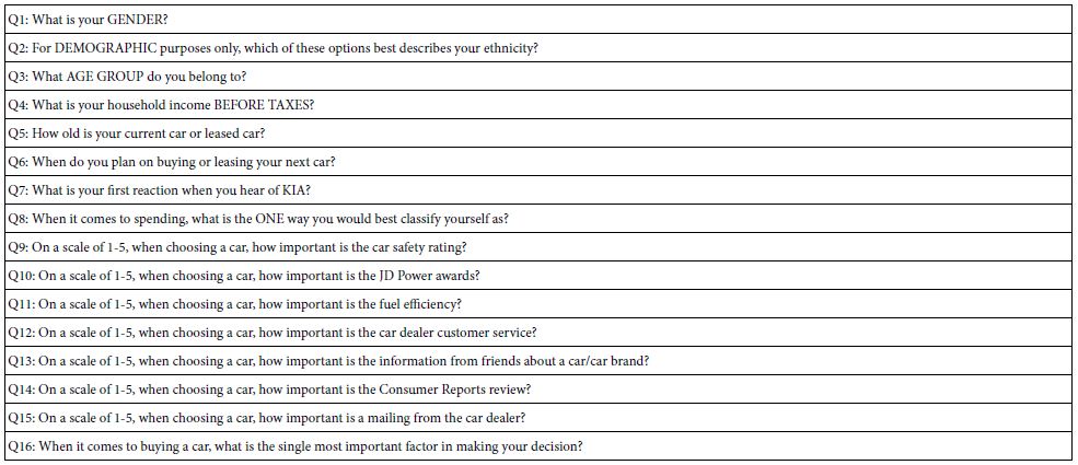
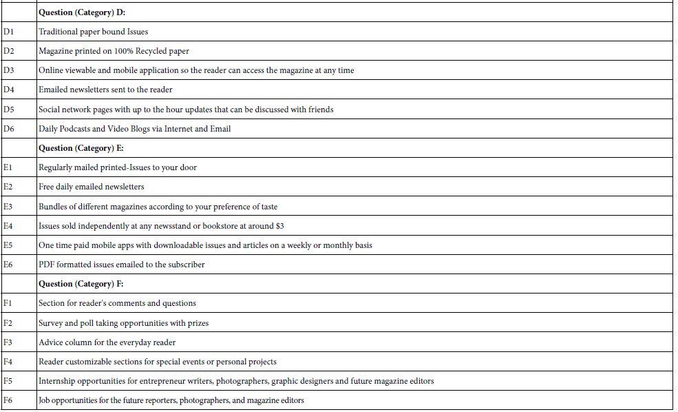
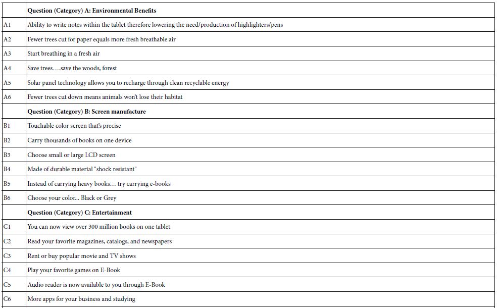
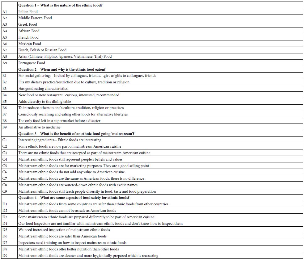
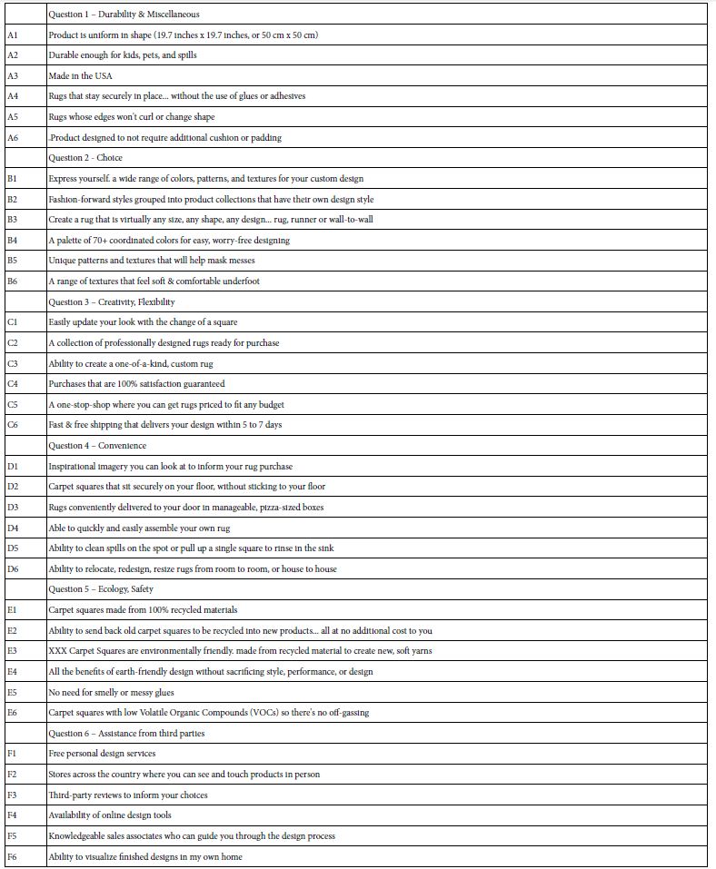
Mind Genomics prescribes a set of inputs, following a template. The templated design selects a certain number of variables (called questions or dimensions). The variables or questions ‘tell a story’. The questions never appear in the study. The questions are used only to guide the researcher who must provide answers to the questions. Sometimes, such as the case with this study, the questions or dimensions are simply bookkeeping tools to make sure that mutually contradictory elements can never appear together in a vignette. For this study, the researchers selected the so-called 6×6 design. as shown in Table 1. The elements are stand-alone phrases, painting a word picture.

Table 1: The six questions and the six elements (answers) for each group (viz. answers). The structure is only a bookkeeping device to ensure that mutually contradictory elements will not appear together in a vignette

3. Use an Experimental Design to Specific the Combinations

Mind Genomics works by presenting the individual with a large set of vignettes created by the experimental design. The design prescribes the precise combinations, doing so in a which makes each element appear equally often, appear statistically independently of every other element, and in a manner that the combinations evaluated by one person differ from the combinations evaluated by another person. This approach, permuted experiment design [18] ensures that the study covers a great deal of the possible combinations. The experiment design combined these 36 elements into 48 vignettes, combinations of element, with the properties that 36 of the 48 vignettes comprised four elements (at most one element or answer from a question). whereas the remaining 12 of the 48 vignettes comprised three elements (again, at most one element from a question).

4. The Mind Genomics System Creates the Test Stimuli to be Evaluated by the Respondents

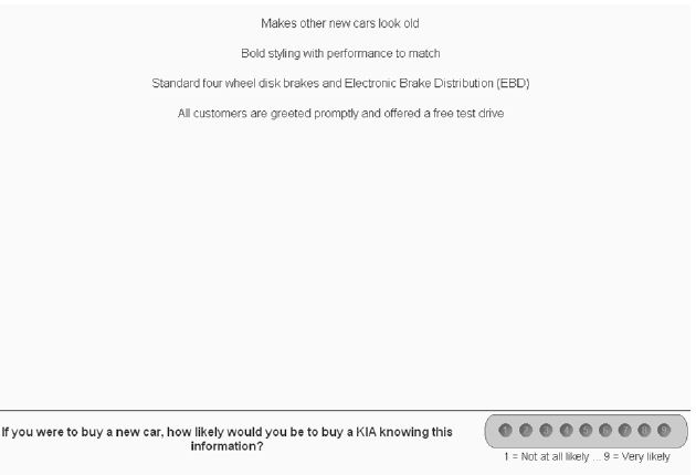
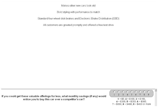
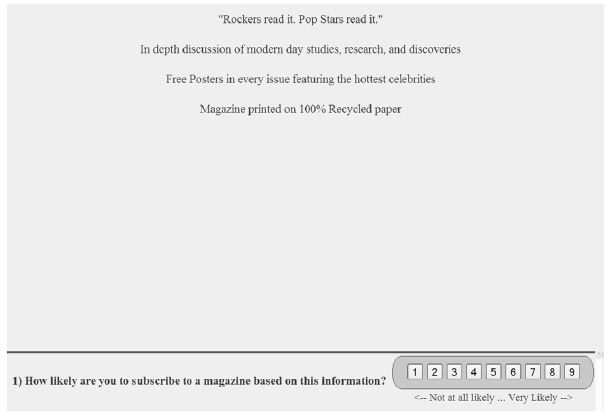
Figure 1 shows one of the vignettes. The vignette seems a haphazard collection of elements, presented in a strange, centered format without connectives. To professional marketers this type of format may best disconcerting. The reality, however, is that the format is exactly what is needed to present the relevant information. The respondent cannot ‘guess’ the right answer. Shortly after the start of the evaluation of 48 vignettes, the respondent stops trying to ‘be right’, and simply responds at an intuitive, gut level. it is precisely this gut response, which best matches the ordinary behavior of individuals faced with the task of selecting a product. Despite the feeling of marketers that their ‘offering’ is special, and engages the customer, and despite the best efforts of advertising agencies their ‘creative’ these mundane situations generate are generally faced with indifference. It is decision within the world of indifference that must be understood, not decision making occurring when a mundane situation is focused upon, and unusual amounts of attention to something that would be simply considered, a decision made, and the person then move on.

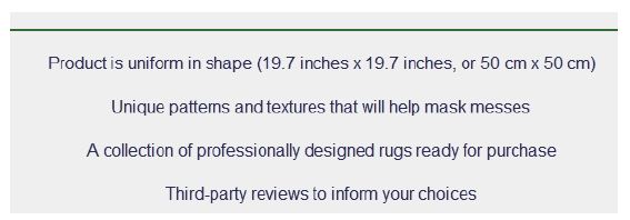
Figure 1: Example of a vignette comprising four elements. The rating scale appears below, showing a 9-point purchase scale (1=Not likely to purchase… 9=Very likely to purchase

5. Orient the Respondents

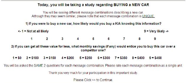
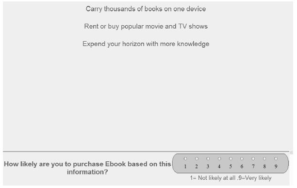
The respondents were oriented by a screen which provided just enough background information to alert the respondent to the nature of the product whose messages were being tested with Mind Genomics. For the purposes of this paper on method, it is not necessary to identify the manufacturer, but it was identified at the actual study. Figure 2 shows the orientation page.

Figure 2: The orientation screen

Analytics

6. Transform the Responses to a More Tractable Form

Our first step of analysis is to consider whether we will keep the 9-point scale, or whether we will change the scale to something more tractable. Most researchers familiar with the 9-point Likert scale, or indeed with any category scale or ratio scale, will wonder why the need for change. It is easier to begin with a good scale, with good anchors and stay with that scale. At the level of science, the suggestion is correct. At the level of the manager working with the data, nothing could be further from reality. Managers are interested in what the scale numbers mean. The statistical tractability of the 9-point scale is a matter of passing interest. It’s the meaning, the usefulness of the data as an aid to make decision which is important.

The conventional approach in consumer research is to transform the data, so that the data becomes a binary scale, yes/no. The manager is more familiar with, and more comfortable with yes/no decisions. There is no issue of ‘what do the numbers’ mean. In the spirit of this ease of use of binary scales, yes/no, the data were transformed. Ratings of 1-6 were transformed to ‘0’ to denote ‘no’, different gradations of not purchasing. Ratings of 7-9 were transformed to ‘0’ to denote ‘yes’. To each of these transformed numbers was added a vanishingly small random number (10^-5). That action becomes prophylactic, preventing any individual respondent from generating all 0’s or all 100’s across the 48 vignettes evaluated by the individual. If the respondent were to rate all the vignettes 1-6, showing variation, the transformation would bring these to 0, and the regression analysis to follow would ‘crash.’ In the same way, were the respondent to rate all vignettes 7-9, the transformation would bring these to 100. In the actual data, 12 respondents generated all 0’s, but 284 respondents generated all 100’s because they found enough appealing in each vignette to assign the rating of 7-9.

7. Relate the Response (TOP3) to the Presence/Absence of the Elements Using ALL the Data

Mind Genomics uses so-called dummy variable regression, a variation of OLS (ordinary least squares regression Hutcheson, 2019). The analysis is first done at the level of the total panel. The independent variables are all 36 elements. Each respondent generates 48 rows of data, each row corresponding to one of the 48 vignettes the respondent evaluated. The data matrix for each respondent comprises 36 columns, one column for each element. The cell for a particular vignette has the number ‘0’ when the element is absent from the vignette, and the number ‘1’ when the element is present. There is no interest in the meaning the element. It is simply a case of being presence (1) or absent (0). The objective of the analysis is to determine the ‘weights’ or coefficients of the 36 elements, from the total panel.

The data are now ready for the first pass, viz., combining all the data into one database comprising 48 rows for each respondent, and 927 respondents. The equation is: TOP3 = k₀ +k₁(A1) +k₂(A2) … k₆(F6). Although the respondent evaluated combinations comprising three and four elements in a vignette, the OLS regression is easily able to pull out the part-worth contributions, the coefficients. The first estimated parameter, k₀, is the so-called the additive constant. The remaining estimated parameters, coefficients k₁-k₃₆, are the weights for respective elements.

The coefficients are additive, viz., they can be added to the additive constant. The combination (additive constant + sum of elements in the vignette) provides a measure of how well the vignette is expected to perform. The only requirement is that the vignette comprises 3-4 elements.

8. Interpret the Results from the First Modeling

Table 2 shows the coefficients for the 36 elements as well as for the additive constant. Note that this will be the only time that the full set of 36 coefficients and the additive constant will be shown, to give a sense of the impact of each element. The Mind Genomics process produces what could become an overwhelming volume of data, the sheer wall of numbers disguising the strong performing elements.

Table 2: Coefficients of the 36 elements, sorted by the value in descending. The three strongest performing elements are shown as shaded cells

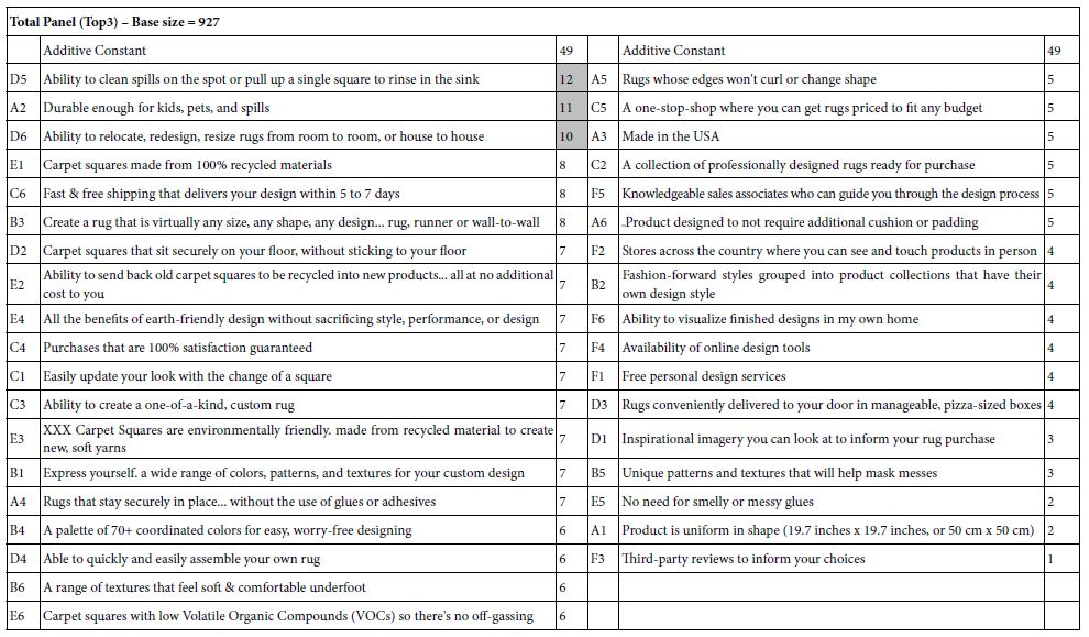
The additive constant, 49, is the estimated proportion of times people will rate the vignette as 7-9 (likely to purchase or very likely to purchase) in the absence of elements. The additive constant is a purely estimated parameter because by design all vignettes comprised 3-4 elements. Nonetheless, the additive constant gives a sense of the predisposition to buy. The value 49 means that about 49% viz., about half the people are likely to say to buy, even in the absence of elements which provide information. The additive constant of 50 is typical for a commercial product of moderate interest. s reference points, the additive constant for credit cards is around 10, the additive constant for pizza is about 65. Our first conclusion is that there is a moderate basic interest in the carpet design squares. The elements will have to do a fair amount of work to drive interest. The ‘work’ comprises the discovery of strong elements.

The coefficients in Table 2 may initially disappoint the researcher because out of 36 elements only three elements perform strongly from the total panel of 927 individuals. There might be at least two things going on to produce such poor performing elements. The first is that the messages are simply mediocre, despite the best effort of copyrighters and professionals to offer what they believe to be good messages. In such a case there is no option but to return to the drawing board and start again. The problem is in which direction, and how? The second is that we are dealing with groups of people in the population, mind-sets, who pay attention to different messages. The poor performance may emerge because we mix these people together, and their patterns of preferred elements cancel each, like streams colliding, preventing each other from continuing on their respective paths. In other words, the poor performance from the total panel may emerge from mutual cancellation of what otherwise be strong performance of some elements.

Clustering the Respondents into Two, Three, and Four Mind-sets

9. Create 927 Individual-levels to Prepare for Clustering into Mind-sets

The permuted experimental design is set up so that each respondent evaluated the precise types of combinations needed to run the OLS regression on the data of that individual. Thus, by running the 927 regressions, one per respondent, one gets a signature of the respondent in terms of the respondent’s mind-set regarding the product. The next step in the analysis runs the 927 different OLS regressions, storing them in a single matrix along with the self-profiling classification that the respondent did at the end of the evaluations.

10. Clustering the Respondents

Clustering is a popular technique to divide ‘things’ by the features that they have. Things, e.g., respondents, can be defined by the pattern of their 36 coefficients. Respondents with similar patterns belong in the same cluster, which will be called ‘mind-set’ because the clusters show what the respondents feel to be important for this flooring product. The respondents may not be similar at all in any way, but they are similar in their pattern of responses in this study.

11. Use K-Means Clustering (Likas et. al., 2003)

K-Means measures the distance between two respondents, based upon the similarity of their 36 coefficients. K-Means clustering tries to maximize the ‘distance’ between the two centroids of 36 numbers each computed on the respondents in the cluster, while at the same time minimize the sum of the pairwise distances within a cluster. ‘Distance’ between two respondents based upon the 36 coefficients was operationally defined as the quantity (1-Pearson Correlation Value). The Pearson correlation takes on the value of 1.00 when the 36 elements are perfectly linearly related to each other, making the distance (1-R)= 0. The Pearson correlation takes on the value 0f -1 when the 36 elements are perfectly inversely related to each other, making the distance (1-R)=2 (1 – – 1 = 2).

12. Interpret the Data

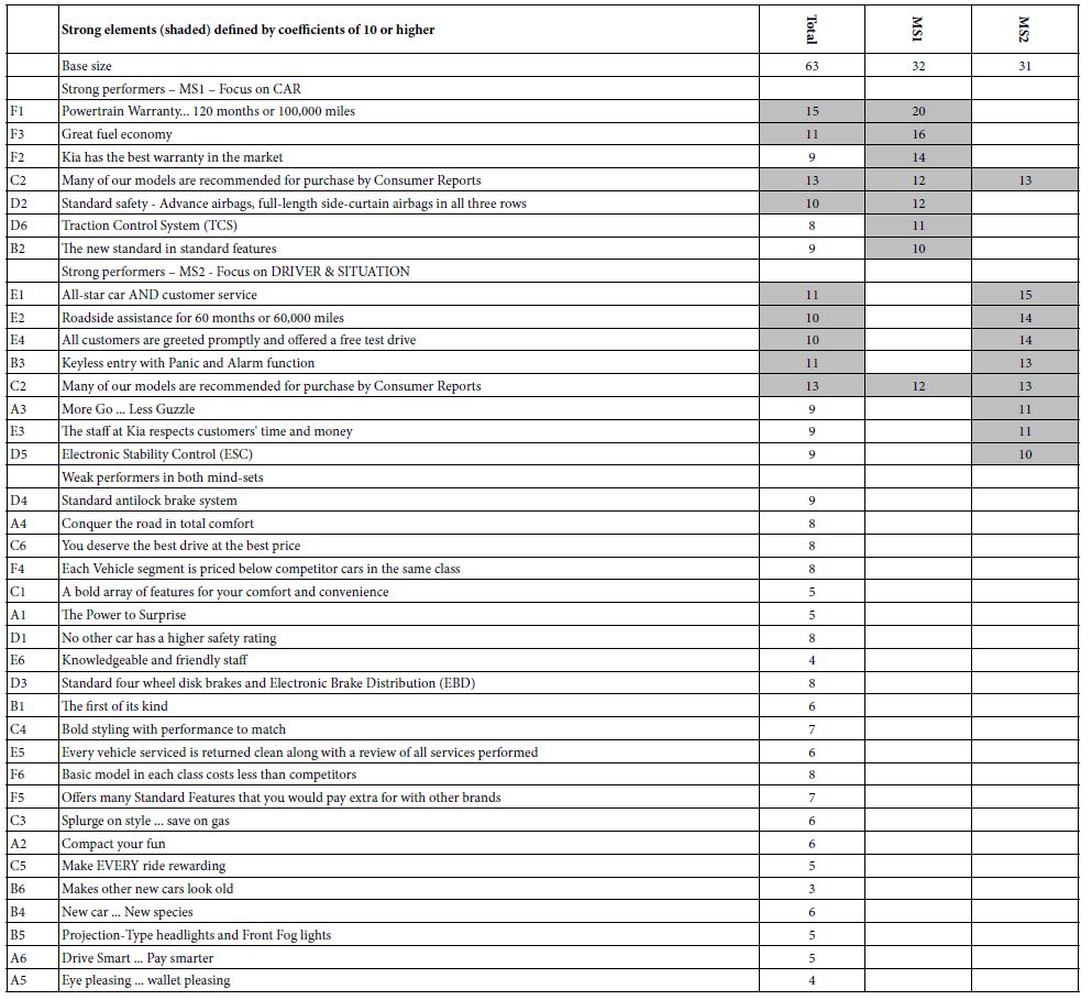
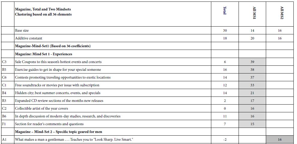
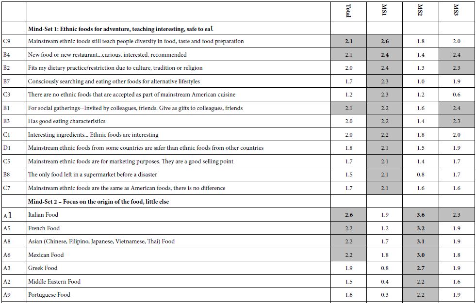
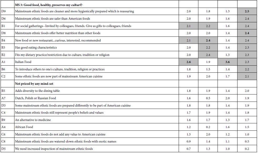
Table 3 shows the strong performing elements from three segmentation exercises: breaking the data into two mind-sets (clusters), breaking the data into three mind-sets,), and breaking the data into four mind-sets . There is an abundance of strong performing element within each cluster. We have created an artificial cutoff point of coefficients of 16 or higher being strong, and coefficients of 15 or lower being less relevant. The reality of the product, and the nature of the respondents presented with a real product show the strong performance of elements, performance hard to obtain with theory-based ideas. For this study, the elements in the table are selling points of real products, relevant to everyday life, not theory-based ideas lacking the life-giving power of reality and everyday importance.

Table 3: Strong performing elements four two, three, and four mind-sets emerging from the clustering the original 36 coefficients

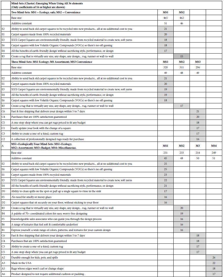
It is important to recognize that the mind-sets are easy to name. The strongly performing coefficients share some ideas in common. Based upon the strong performing elements one gets a sense of the respondent’s way of thinking in each mind-sets. it is also important to note that there is no ‘one correct’ number of mind-sets. The mind-sets tend to repeat but increasingly finer distinctions emerge between and among mind-sets as the number go from two to four

From 36 Down to 6 – Can We Improve the Clustering by Creating Fewer but Uncorrelated Predictors?

13. Hypothesis Based Upon the Efforts to Find ‘Primaries’

Although the 36 elements were put together in a way which may their appearances statistically independent of each other, the reality is that the elements might be skewed to one or another aspect, such as fewer elements in one topic area, and many more elements in another topic area. The Mind Genomics system tries to instill a balance in the nature of the elements used by forcing an equal number of elements or answers for each question. That strategy works for academic subjects but may not be the appropriate when the businessperson is trying to understand the mind of the customer.

With 36 elements, it may be advantageous to reduce the number of elements to a smaller set of ‘pseudo-elements,’ mathematical entities called factors which are uncorrelated with each other [19]. The application of principal components factor analysis to these data, with a moderate but not severe criterion for extracting a factor (eigenvalue > 2) produced a set of six uncorrelated ‘pseudo elements,’ the factors. The six emergent factors were uncorrelated with each other by the process of factor analysis. The factor structure was further simplified by rotating the six factors to a simple form, using Quartimax rotation. Finally, each of the 927 respondents become a point in this new six-dimensional space, where the rotated factor because the new ‘elements’, and thus name pseudo elements.

A Technical Note

The method of reducing the 36 elements to uncorrelated factors involves a great number of alternative choices, as does the method for creating the clusters of mind-sets. This paper simply chooses one way for exploratory purposes. Other factor analyses decisions might lead to different clusters, and a different decision. The foremost stated, this exploration is simply looking at a possible way to improve our knowledge emerging from the experiment, not as a method for ultimate discover of the ‘one array of mind-sets.

14. Interpret the Data

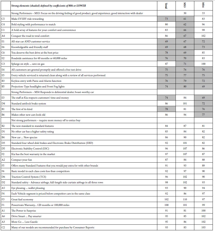
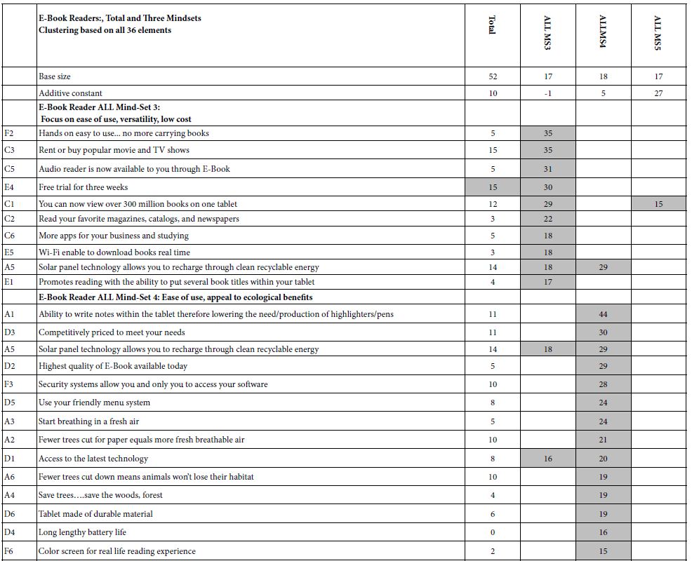
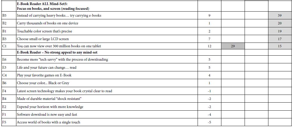
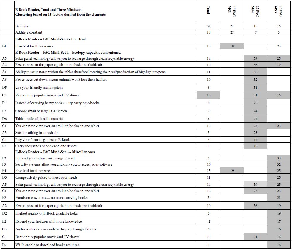
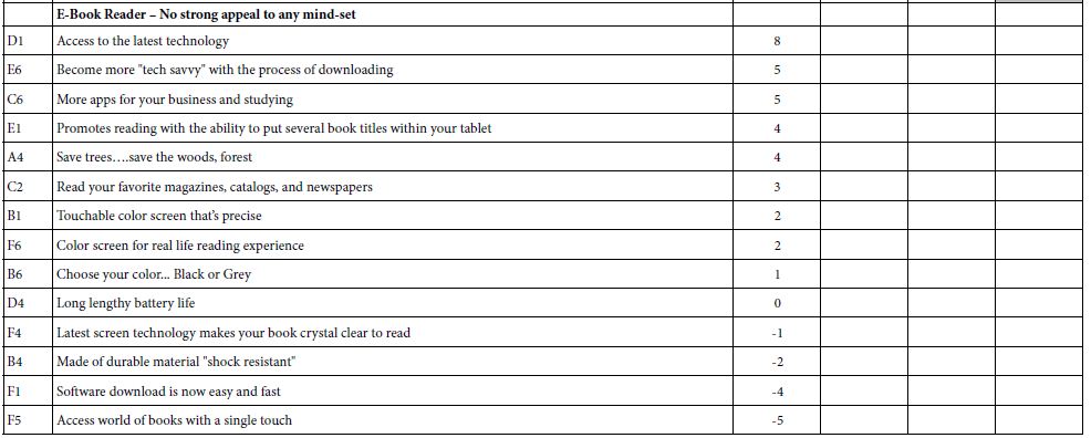
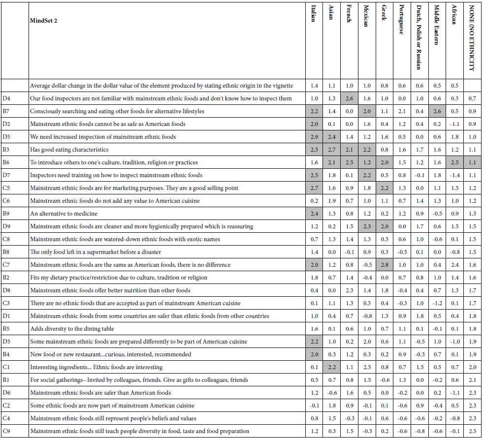
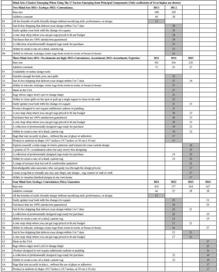
Table 4 recreates the two, three, and four mind-sets, this time using the clustering based upon the six factor scores of each of the 927 respondents, rather than on the original 36 coefficients for each of the 927 respondents. The results at first look promising in terms of many more elements emerging.. We see several interesting departures from what we saw in Table 3, which showed the same clustering, but with the full set of 36 coefficients. Returning to Table 4 we see that one of the additive constants is always high, suggesting that there is one mind-sets which is strongly predisposed to the items. Generally, this group will respond to most elements because their basic interest is high. The other one, two or three mind-sets show much lower constants, but many strong performing elements. The second observation is that these mind-set created after factor analysis are harder to name, because they comprise many more elements. The greater number of viable elements may have emerged because the additive constants are low, however.

Table 4: Strong performing elements among four two, three, and four mind-sets emerging from the clustering the six factor scores emerging from the 36 coefficients

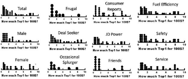
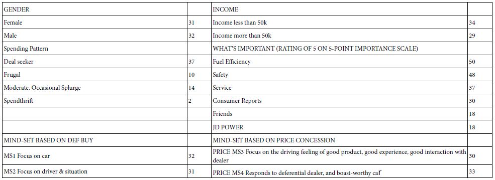
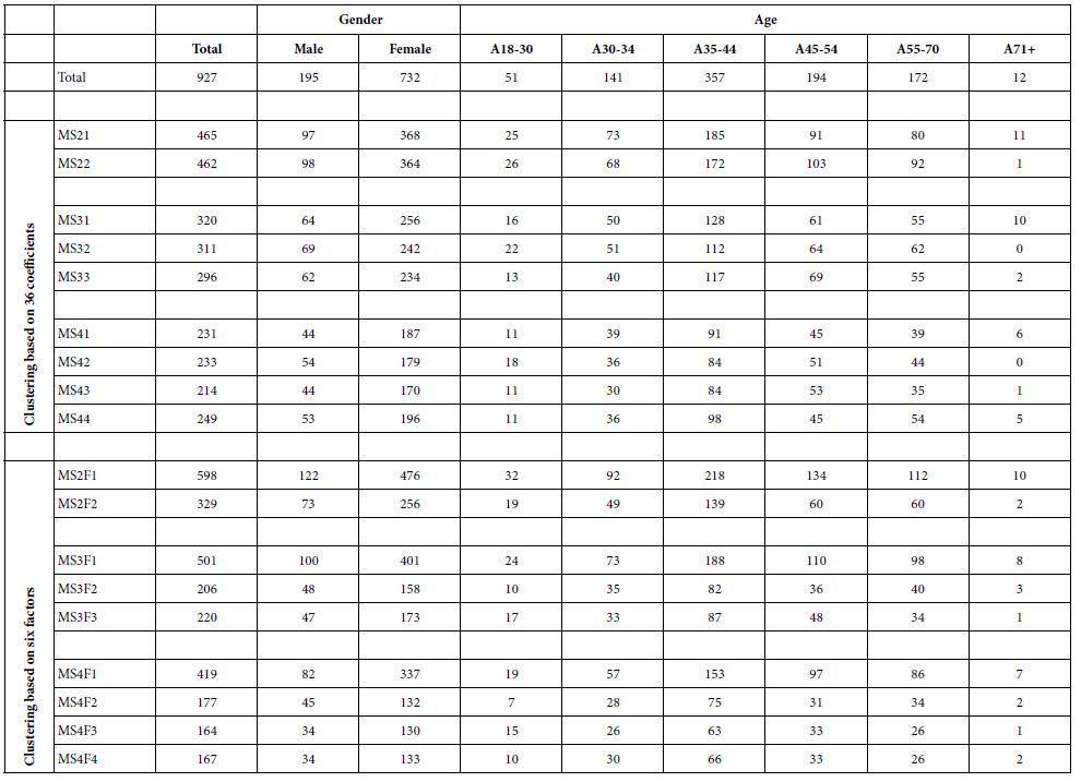
15. Basic Composition of Mind-sets, Gender and Age

Mind Genomics continues to reveal that there is no simple relation between who a person IS and the mind-set to which a person belongs. Table 5 shows the composition of the mind-sets, by gender and by age. The patterns which emerge from Table 5 can be augmented by much more in-depth tabulations, beginning with more details about WHO the person is, what the person DOES at home regarding home decor, attitudes and behavior regarding SHOPPING, and so forth. The important thing is that by knowing more in-depth about the respondents, as well as the respondent membership, it might be possible to assign a new person to one of the segments.

Table 5: composition of the mind-sets by gender and by age, respectively

Discussion

16. The thrust of this paper is methodology, the study of method in the true sense of the word. The effort to understand method began with a simple question, ‘how many clusters or mind-sets to extract.’ It devolved into two questions of the same sort, one dealing with extracting mind-sets with the elements as is, and the other with extracting mind-sets after the elements have been reduced to orthogonality through factor analysis. And finally, the third and not directly stated question, why do the elements score so highly in this study, whereas in most Mind Genomics studies the elements rarely score this highly.

17. Question 1: Why do These Elements Score So Well, When in Most Mind Genomics Studies the Elements Score Poorly?

The answer to this comes from two aspects and can be best considered as conjectures. The topic of floor coverings is interesting, comprising interesting stand-alone elements which educate and intrigue people. In contrast, most of the topics worked on by Mind Genomics are more generic, deal with topics that are not so interesting, and fail to incorporate engaging information to present to the respondent. So, for the first answer the conjectures are we are dealing with an interested population, in a topic which can provide interesting information, rather than dealing with a topic whose ideas are usually watered down so that they provide little ‘juicy’ information to think about. In other words, it may be that conventional studies are simply bland.

18. Question 2: How Many Mind-sets to Extract

When we look at Tables 3 and 4, the results from the clustering our issue is that we just don’t know whether we should opt to call the mind-set by the most prevalent type of element in the mind-set, or whether we should accept the mind-set as comprising a mélange of different meanings. This problem of a mélange of different meanings will stop being a problem when we end up allowing six, seven eight or more clusters.

19. In the words of Harvard’s eminent psychology and founder of Modern-day Psychophysics, S.S. Stevens (d. 1973) ‘Validity is a matter of opinion.’ In Stevens’ words, as long as the experiments are performed correctly the answers are valid. All four solutions, Total, two, three and four mind-sets, would be equally valid if one were dealing with stimuli having no cognitive richness. The clustering algorithm does not pay attention to the underlying nuanced meanings of the element. If we were to assume that the elements are in some unknown language, and we extract two, three and found mind-sets, which solution would be correct? All would be equally valid in mathematical terms.

20. The issue is quite different when we work with elements. These elements have a great deal of meaning, cognitive richness. When we extract the clusters, we can look at the meaning of the element, and from the meaning decide upon the nature of the cluster. Based upon Table 3 the best strategy is work with four mind-sets, if these mind-sets can be identified. Each mind-set focuses on a different aspect of floor materials.

21. Question 3: Do Orthogonal Variables, Presumably Balancing Out Different Ideas, Produce More Interpretable, Tighter Clusters or Mind-sets?

Is it better to work with the original set of elements when creating mind-sets, or should we reduce the elements to a set of mathematically independent variables, such as our six factors? Table 4 suggests that it was difficult to find a simple guiding theme for each cluster or mind-set, despite the emergence of high positive coefficients. As a result, it is probably better to work with the original set of elements, and not perform the factor analysis to produce a smaller group. In the end, we want to make sure that the mind-sets we identify are real and meaningful, and that the combinations generated from these mind-sets make sense and score as high as possible.

References

1. Kamtekar R (2013) Plato: Philosopher-Rulers. In: Routledge Companion to Ancient Philosophy (pp. 229-242). Routledge.
2. Bayer G, (1998) Classification and explanation in Aristotle’s theory of definition. Journal of the History of Philosophy 36: 487-505.
3. Gajanova L, Nadanyiova M, Moravcikova D (2019) The use of demographic and psychographic segmentation to creating marketing strategy of brand loyalty. Scientific Annals of Economics and Business 66: 65-84.
4. Wells WD (1975) Psychographics: A critical review. Journal of Marketing Research 12: 196-213.
5. Garreau J (1981) The Nine Nations of North America. Avon Books.
6. Webber R, Sleight P (1999) Fusion of market research and database marketing. Interactive Marketing 1: 9-22.
7. Moskowitz HR, Gofman A, Beckley J, Ashman H (2006) Founding a new science: Mind Genomics. Journal of Sensory Studies 21: 266-307.
8. Moskowitz HR, Silcher M (2006) The applications of conjoint analysis and their possible uses in Sensometrics. Food Quality and Preference 17: 145-165.
9. Carroll JD, Green PE (1995) Green Psychometric methods in marketing research: Part I, conjoint analysis.” Journal of marketing Research 32: 385-391.
10. Gofman A, Moskowitz HR (2010a) Improving customers targeting with short intervention testing. International Journal of Innovation Management 14: 435-448.
11. Goldberg SM, Green PE, Wind Y (1984) Conjoint analysis of price premiums for hotel amenities. Journal of Business S111-S132.
12. Green PE, Krieger AM, Wind Y (2001) Thirty years of conjoint analysis: Reflections and prospects. Interfaces 31: S56-S73.
13. Wind J, Green PE, Shifflet D, Scarbrough M (1989) Courtyard by Marriott: Designing a hotel facility with consumer-based marketing models. Interfaces 19: 25-47.
14. Laparra-Hernández J, Belda-Lois JM, Medina E, Campos N, Poveda R (2009) EMG and GSR signals for evaluating user’s perception of different types of ceramic flooring. International Journal of Industrial Ergonomics 39: 326-332.
15. Macias N, Knowles C (2011) Examining the effect of environmental certification, wood source, and price on architects’ preferences of hardwood flooring. Silva Fennica 45: 97-109.
16. Roos A, Hugosson M (2008) Consumer preferences for wooden and laminate flooring. Wood Material Science and Engineering 3: 29-37.
17. Zamora T, Alcántara, E, Artacho MA, Cloquell V (2008) Influence of pavement design parameters in safety perception in the elderly. International Journal of Industrial Ergonomics 38: 992-998.
18. Gofman, Alex, and Howard Moskowitz (2010b) Isomorphic permuted experimental designs and their application in conjoint analysis. Journal of Sensory Studies 25: 127-145.
19. Cureton EE, D’Agostino RB (2013) Factor Analysis: An Applied Approach. Psychology Press.

DOI: 10.31038/PSYJ.2022414

Abstract

In two separate experiments, groups of 50 respondents evaluated vignettes comprising systematically varied combinations of elements, experiment 1 dealing with the content of magazines, experiment 2 dealing with the features of an e-book reader. The vignettes were evaluated on 9-point Likert scales. Equations relating the presence or absence of the 36 elements in each experiment revealed unusually high coefficients. Clustering the patterns of coefficients revealed two mind-sets for the magazine contents, three mind-sets for the e-book reader. The mind-sets were not diametrically opposite, in the way the clustering would show for most products. Rather, the mind-sets suggested different patterns of preference, instead of preference/rejection. The argument is made that for many products with positive features, mind-set segmentation will reveal groups differing in the order of preference, with most features liked, rather than revealing the more typical finding that the mind-sets exhibit strong and opposite patterns of acceptance/rejection.

Introduction

The 21^st century abounds in media, formerly just printed and broadcast, now electronic. Over the past decades readers have been introduced to the benefits of e-readers, virtually small computers created for the presentation of written material of many sorts, from books presented as searchable files, to pictures, presentations, to audio books, and the like. At the same time, the 21^st century abounds in the printed word, on traditional media, such as newspapers, magazines, books, and so forth.

The focus of the two studies reported here was on the response to magazines (study #1), and to e-book readers (study #2), from the point of view of first- and second-year college students entering the world of higher education. The idea was to find out what features they thought would be relevant to people, and in turn, how people felt about combinations of these features in small vignettes (descriptions of offerings) and evaluated by respondents.

The academic literature as well as the business literature focuses on who reads magazines [1] and who uses e-book readers and the reasons [2-6]. The studies on media give one a sense of looking from the outside in, from the point of view of a third-party observer trying to make sense of a situation and reporting on the various features of situation. The observer is describing what she or he sees, and the potential organizing patterns which might be emerging, based what is observed, and the intuition of the observer. There is a sense of the ‘inside of the mind’, but not a feeling of immediacy, the type of immediacy when one reads a description of a product or service, and feels an excitement, a sense of ‘that’s just what I want.’

Rationales for the Two Studies Reported Here

The original studies were conducted as part of a set of studies at Queens College, (CUNY, NY), by students turned experimenters. The focus was on exploring the world of the everyday. One remarkable event emerged from the two studies. The study magazines were perceived by many of the respondents as fairly boring. Many of the elements were simply uninteresting, and in fact 22 of the respondents did not end up liking anything in that was being offered. In contrast, all the elements in the e book reader were considered interesting. Thus, it was of interest to compare the two.

The Mind Genomics process makes what was a typical questionnaire into an experiment. The questionnaire and the experiment both try to uncover what respondents feel to be important. The questionnaire works by presenting the respondent with a single set of stimuli, messages or elements presenting different ideas, and analyzing the ratings. The stimuli may be of the same type, presenting alternatives of a single idea, or the stimuli may be of entirely different categories of messages. In contrast, Mind Genomics can be said to an experiment in which the respondent rates combinations of messages, simulating a typical reality [7-9].

The approach is illustrated by a series of steps, each step comparing the two studies.

Step 1: Select the Topic, the Questions, and the Answers (elements)

Mind Genomics works with the experience of the everyday. It is critical, therefore, to select a delimited topic, and create a story framed by questions, in the manner that a story might be related by a person. The questions provide the structure to move the story forward. The story need not be the type of story with a plot. Rather, the story merely needs to provide a set of smaller ‘sub-topics’, aspects of the main topic, but aspects that can be dealt with by simple stand-alone phrases which ‘describe.’ The topic will be introduced to the respondent, so the respondent knows to what the test stimuli pertain. Th questions are never shown to the respondent, but simply serve as an aid to creating the answers, the elements, which will be shown to the respondent in test combinations.

Table 1A shows the structure of topic, questions, and answers for the magazine, something with which people were very familiar at the time of the study, in 2012. The topic was particularized to a subscription to the magazine, rather than interest in general in the magazine. The elements would be looked at in the light of a call to action, to subscribe or not to subscribe to the magazine.

Table 1A: Questions and answers (elements) for the magazine

Table 1B shows the structure of topic, questions, and answers for the E-reader. At the time of the study, E-readers were coming into vogue. Amazon had introduced the Amazon Kindle series, E-book readers, so the product idea was becoming better known. Technology was evolving quickly. The focus of the study was features and capabilities of the product.

Table 1B: Questions and answers (elements) for the E-Book Reader.

Allowing people to collaborate, especially students who are as yet unfettered by the cynicism of adults, generates ideas which run the gamut. The elements shown in Tables 1A and 1B emerged from students, not from professional copyrighters, not from professional ‘creatives’ whose job it is to come up with winning ideas. The Mind Genomics system encourages the exploration of new ideas, often ideas in the mind of young people. It will be interesting to measure how well these ideas perform. they are certainly different from many of the tried-and-true ideas proffered as the output of professionally moderated creative session. The performance will be measured empirically below

Step 2: Combine the Elements into Short, Easy to Read Vignettes, Using Experimental Design

Mind Traditional efforts to teach the ‘scientific method’ are founded on the belief that a variable must be isolated, and studied, but only after all of the possible variation, the ‘noise’ around the variable has been eliminated, either by suppressing the noise (testing the element by itself i the simplest form), and/or by averaging out the noise (e.g., testing with dozens or even hundreds of people, so that the individual variation averages out).

Mind Genomics was founded on the basic tenet judgment data of real-world stimuli should be done in a way which best resembles the real world, namely mixtures.,,, namely identify the variables to be tested, combine them in a way which resembles th type of compound stimulus which one encounters in nature. By combining the different elements in structured way, using an experimental design, which mixes and matches the different independent variable, one presents the respondents with more realistic test stimuli. We encounter mixtures all the time and react to them. Thus, the mixtures tested by the respondents are more similar to what the person would face. The key difference is that the experimental design permits the research to deconstruct the reaction to this ‘combination’ into the contributions of the components, the variables of interest.

The requirements for a Mind Genomics experimental design are that the elements should appear equally often, that the vignettes be ‘incomplete’ (viz., some vignettes are absent elements or answers from a question), that the elements be statistically independent of each other, and the experimental design be valid down to a base size of one respondent. Finally, the experimental design be permutable, so that by permuting elements or answers in a single question new combinations emerge, based upon the same design structure [10].

It is important to note that with the foregoing approach, each respondent evaluates a different set of 48 vignettes, prescribed by the underlying experimental design (called the 6×6 design; six questions, six answers or elements per question). With 50 or so respondents, there are 50×48 or 2400 vignettes evaluated by the respondents, most of which are different from each other. In that way the Mind Genomics system is metaphorically like the MRI machine, which takes pictures of the same tissue from different angles and combines these pictures by computer to arrive at a single 3-dimensional image of the underlying tissue.

The output of the experimental design appears in Figure 1A, showing a vignette for the magazine, and Figure 1B showing a vignette for the e-book reader.

Figure 1A: Example of a four-element vignette for the magazine study

Figure 1B: Example of a 3-element vignette for the e-book reader

Step 3: Execute the Mind Genomics Study on the Internet

Beginning in the late 1990’s, a great deal of consumer research migrated to the web, to the internet. Companies found that the data generated by web-based interviews seemed to be just as valid as data generated by in-person interviews and mailed-out paper questionnaires. Establishing web-interviews as a valid way, and indeed far less expensive way, to obtain data gave a boost to interviews which need technology embedded in their backbone. Min Genomics is one of the approaches which proposed, because each respondent was to evaluate a unique set of elements. The only practical way was to have a computer combine the elements in ‘real time’, following the underlying 3expeirmental design. The process became streamlined over time. The respondent would log in, following a link, be presented with an orientation screen, and then a set of systematically varied combinations, created ‘in real time’, at the site of the respondent’s computer.

Figure 2A shows the orientation screen for the magazine study, Figure 2B shows the orientation screen for the e-reader study. The respondents were recruited by an online panel provider, Turk Prime, Inc. which provided respondents in the United States. The compensation to the respondents was set by Turk Prime, Inc. as part of their internal policies. These policies as well as the identification of the respondents, were not available through the service. The only guarantee was that the respondents were vetted by Open Venue Ltd., part of their panel.

Figure 2A: Orientation for the magazine study

Figure 2B: Orientation screen for the e-reader study

Figures 2A and 2B show the orientation screen. Very little information is given regarding the purpose of the study, and the rationale for selecting the elements. Just the topic is given. The rest of the screen provides information about the number of question (two), and the type (scalar, Likert Scale for Question 1, presented here; selection of emotion for each vignette, not presented here).

The orientation screen goes out of its way to reassure the respondent that all the screens are different from each other, and that the study will take 10-15 minutes. These two reassurances were put in after the early experience on the Internet, when respondents kept saying upon exist that the concepts they evaluated seemed to have many repeats (not possible with the design), and that they wanted to know how long the interview would be. Rather than giving a precise time, it was deemed better to give them a reasonable range of 10-15 minutes. Most respondents finished earlier.

Observations of respondents doing these types of studies in a central location revealed that the respondents often begin by trying to ‘outsmart’ the research, trying to figure out the appropriate answer. With single elements rated, this outsmarting or gaming the system is possible. With 48 different combinations, however, it is impossible for the respondent to game the system. The respondent may begin with an effort to outsmart the system, but almost universally the respondent relaxes, and simply answers in what the respondent feels is an uninterest way, barely paying attention. That tis precisely the right state for the respondent, because in that state the answers come from the heart, without being edited to be politically correct.

Step 4 – Acquire the Data and Prepare It for Analysis

Each respondent evaluated 48 difeferent vignettes, consturcted according to an experimental deesign. The respondent first rated the vignette in terms of interest using a 9-point category or Likert Scale (subscribe fo the magazine, purchase for the e-book reader). The respondent then ratedthe vignette in terms of emotion experience after reading the vignette. Those data are not presented here.

The foundations of Mind Genomics lie in the fields of experimental psychology, consumer research, and statisitics, respectively. Experimental psychologists do not usually convert the data from the Likert Scales, preferring the granularity, which allows statistical analysis to uncover more statically significant effects using tests of difference. In contrast,, users of Mind Genomics data, typically managers want to use the data for decision making (e.g., use/not use; go/don’t go). It is important for them to interpret the data to make their decision. All too often, the manager presented with averages across people from a projecting using Likert Scalesw will begin the interaction by asking a question like ‘what does a 6.9 average on the rating scale ‘mean’, and what should i do?’

The tradition in consumer research and in Mind Genomics, followed here, transforms the Likert sale to a two point scale, 0 and 1 or 0 and 100, repectively. They two transformed scales, 0-1, 0-100, are different expessions of the same data, but present the data either with decimals (0-1), or without decimals (0-100), We chose the 0/100 tranfomration,  Ratings of 1-6 were coded 0, ratings of 7-9 were coded 100, and a vanishingly small random number (<10^–5) was added to make sure the transformed rating would always have variation acfrosss the 48 vignettes for a single respondent. This prophylatic measure ensure that one could use regression modeling at the level of the individual respondent, even in those cases when the respondent confined the ratings to one region, viz., 1-6 or 7-9 respectively.

Step 5 – Create Individual Level Models, through Regression, Relating the Presence/Absence of the Elements to the Transformed Response

It is at Step 5 that the real analysis begins, an analysis which is virtually mechanical in nature, yet which repeatedly shows how the consumer mind makes decisions. The data were prepared in at Step 4. Step 5 uses OLS (ordinary least squares) multiple regression to relate the presence/absence of the 36 elements to the transformed rating. The equation is expressed as:

Binary Transformed Rating = k₀ + k₁(A1) + k₂(A2)….k₃₆(F6)

For those respondents whose ratings were all between 1 and 6, the coefficients were all near 0 an the additive constant was around 0 as well. For those respondents whose rating whose ratings were all between 7 and 9, the coefficients again were all near 0, and the addiive consatn was around 100. Out of 52 respondents, 22 respondent showed this pattern for magazine, none showed this pattern for e-book reader. The data from these 22 respondents were eliminated from the database, leaving only respondents who showed variation in their transformed binary response.

Step 6 – Cluster the Respondents into Either Two Groups (Magazine) or Three Groups (e-Book Reader)

Step 6 attempts to divide the respondents in a study into clusters, doing so that the the respondents in a clusters are ‘similar’ to each other, while at the same time the pattern of the 36 averages of the coefficients are very different between two clusters or very different across three clsuters. The process can be done very easily using k-means clustering [11]. The clustering program returns with the assignment of each respondent to exactly one of the two clusters (for magazines), or one of the three clusters (for e-book readers). Afterwards, run one equation for all the respondents in a study, and two separate equations for all respondents in each of the two mind-sets (magazine), three separate eqations for all respondents in each of the three mind-sets (e-book reader).

The clustering procedures are mathematics-based, attempting to bring some definable order into what might otherwise be a blooming, buzzing confusion, in the words of noted Harvard psychologist, William James. The clusters themselves do not have any concrete reality, but simply represent intuitively reasonable ways to divide objects. Clustering can be done on anything, as long as the measure(s) are comparable across the different objects.

When we look at the clusters, recognizing that we are dealing with a mathematically based system, our judgment should be based on at least two criteria. The first criterion is parsimony. We know that we will get perfect clustering if each of our respondents becomes her or his own cluster. That would defeat the purpose. The idea is to create as few clusters as possible, to be as parsimonius as possible, even at the cost of some ‘noise’ in the system which makes the clustering far less than perfect. Thus, the first rule is the fewer the number of clusters, the better. The second criterion is interpretability, that the clusters should each tell a story. One may want the story to be tight, meaning more clusters, and less parsimony. Or one may allow the story to be less tight, with more open issues, but with more parsimony, viz., fewer clusters. It is always a trade-off; more parsimony versus more interpretability. There is no right answer. In this study, the effort will be towards parsimony, given the range of possible elements that can fit either in a magazine or an e-book reader [12].

One last issues remains to be mentioned. That issue the nature of the variables (elements) considered in the clustering. The traditional approach in Mind Genomics has been to use the coefficients of all of the elements, but not to use the additive constant. There is always the potential that the clustering might be unduly affected by the nature of the elements selected. With 36 elements, one would hope that the elements deal with different aspects in equal ways. But what happens, for example, if most of the elements deal with usage, and only a few elements deal with product features? Would that generate the same clusters were the elements to be configured differently, with only a few elements dealing with usage, and most elements dealing with product features? In other words, is the mind-set segmentation affected by the distribution of the topics dealt with in the study?

To answer the foregoing question, the nature of the variables used in clustering, each study was analyzed twice, AFTER the respondents with all coefficients around the value 0 were eliminated from the data. The first clustering was done with the original 36 coefficients. Both studies comprised featured six sets of six elements each, so the clustering was similar.

The second analysis reduced the dimensionality of the 36 elements using principal components factor analysis [13]. Even though the 36 elements were statistically independent of each other by design, the pattern of 36 cofficients shows substantial co-variations, simply because the elements were similar, generated similar patterns. The PCA isolated eight factors for the magazine subscription, and 15 factors for the e-book reader. The nature of the factors is not important. Rather, the factors are statistically independent of each other. The factors were rotated by Quartimax to make the data matrix as simple as possible. Each respondent was then located in the 8-dimensional factor space for the magazine, or the 15-dimensional factor space for the e-book reader. After the factor spaces were creatd, the clustering was done again, with two mind-sets extracted for the magazine

Step 7: Interpreting the Results – Magazine

Table 2A shows the results for the magazine based upon the clustering into two groups. Three groups did not produce any clearer result. The “Total Panel” data shows all coeficients, positive and negative. For these results, we show only the very strong positive coefficients, 15 or higher.

Table 2A: Coefficients for the magazine, for total and two mind-sets, based on using all 36 elements for clustering.

The three groups, Total, Mind-Set 1 and Mind-Set 2 generate similar, low values for the additive constant, 16-20. The additive constant is the conditional probability of a person wanting to subscribe to the magazine in the absence of elements. The underlying experimental design ensured that each vignette would comprise 3-4 elements, never zero elements. The additive constant is a convenient parameter, estimating the intercept, the likely score in terms of ‘top 3’ that would be obtained in the impossible case of a vignette with no elements.

Table 2B shows the same type of analysis, this time based on the factors of the respondents on eight independent factors (dimensions), rather than on 36 elements.Comparing the two types of segmentation, first based on all 36 elements and the second based on the elements after factor analysis, it is clear the the clustering generates clearer results when the original data is used, confirming the insights of others focused on thepractical uses, opportunities, and pitfalls encountred in clustering [14,15]. In reality, Table 2A, based on all 36 elements, suggests one major mind-set, those interested in experiences. The other mind-set barely enters the picture, only with one element, which scores near the bottom cutoff. Table 2B shows the same pattern as well [16].

Table 2B: Coefficients for the magazine, for total and two mind-sets, based on using all eight factors for clustering, factors derived from the 36 elements.

The final notworthy finding in this study of magazine content is the unusually large number of very strong elements, nine of thirty-six, one quarter, having coefficients of +15 or higher. This is an unusual finding, and may well be attributed to the creative abilities of younger people, ages 17-23, focusing on what is important to them. What is important is the specific, the concrete, the focused feature, not the grand abstraction that a marketer or ‘creative’ in an agency would propose as a coherent, summarizing theme. The responents want specifics.

Step 8: Interpreting the Results – E-Book Readers

Table 3A shows the results for the E-book reader based upon the clustering into three groups. Unlike the findings for the magazine, the three mind-sets for the E-Book Reader made sense. Once again we see low additive constants. When we divide the respondents into mind-sets based either upon the original 36 elements or upon the 15 factors emerging, we see two very low additive constants, and low additive constant around 27.

Table 3A: Coefficients for the magazine, for total and three mind-sets, based on using all 36 elements for clustering.

Table 3B: Coefficients for the magazine, for total and three mind-sets, based on using all 15 factors for clustering, factors derived from the 36 elements.

Like the results for magazines in Tables 2A and 2B, we find that some coefficients are quite high, some of the highest ever recorded for a Mind Genomics study. The hypothesis proferred in the previous section may still hold, viz., that having young, colleage-age students, create the elements is the secret to strong performing elements. It may be that the students think in a more concrete, feature-oriented way, a way which generates a great deal more interest than professional creatives who may think of ‘grand solutions’, rather than of specific features. It may also be that the topic of e-book readers is by its nature simply far more interesting, and au courant

Discussion and Conclusion

Why High Coefficients?

The most surprising outcome from these two studies is the emergence of elements with exceptionally high coefficients. The studies were run in 2012, a decade ago, but that does not provide an explanation for the strong positive coefficients. Hypotheses about in the absence of fact. We have only two examples. What are common about them is that the elements are provided by young people (ages 18-21) rather than by professionals, viz., the so-called highly paid ‘creatives’ in the marketing companies and advertising agencies. and the topics talk to presentations of information, capabilities given to the reader or the user That is, the elements are fundamentally ‘interesting’ to the reader, not just simply recitations of what is. There is a sense of ‘excitement’, perhaps because we are talking about items with clearly interesting, people-oriented features. There are no elements dealing with ‘good practices’, elements that might be necessary in an offering but elements which really do not convince.

The notion that the topic is interesting certainly has merit in the world of Mind Genomics. Most Mind Genomics studies deal with social or medical issues, issues that are not ‘interesting,’ nor issues that people would pay for. Social problem, medical problems are issues about which one gathers information. The elements in this study are used to excite a buyer to buy the product. There is no sense of elements put in because they are legally necessary, or for completeness as one of recommended best practices.

Polarized versus Non-polarized Mind-sets

As noted above, the unusually high coefficients emerging from the total panel for some elements , and the exceptionally high coefficients emerging several times from the separate mind-sets, suggest that we are dealing with a new type of preference pattern, not frequently seen in Mind Genomics, but one easy to recognize. We are dealing with what one might call the ‘pizza phenomenon’. Most people love pizza. It is the toppings which differentiate people. For most people it’s a matter of order of preference, which varies from person to person. The result is that the total panel generates strong liking of the pizza, with the differentiator being the rank order of preference of the topping. There are people who actively dislike certain toppings, but for the most part the mind-sets that would emerge from a study of pizza and those representing different rank orders of items already liked.

In contrast to the above, the pizza phenomenon, where the mind-sets are simply patterns of liking of the same elements, there are those situations where the person likes one element but hates another This pattern is very different from the pizza pattern. The pattern is more similar to the pattern of likes and dislikes of flavors. Flavors themselves strongly polarize people. Some people love a certain flavor, whereas others hate the flavor. One hears those words again and again.

Let’s move this analogizing to the topics of e-book readers and magazine subscriptions. For the most part the coefficients are positive. There are relatively few elements which are strongly negative. There are no moderately negative elements for the e-book reader. Here are the most negative elements for the magazine

C4      Sneak Previews of the upcoming year in music and entertainment          -6

A3      Executives read it . . Uneducated ones look at the pictures             -6

D5      Social network pages with up to the hour updates that can be discussed with friends      -7

A2      Rockers read it. Pop Stars read it.       -9

The patterns emerging for both the magazine (less so) and the e-book reader (more so) is that the creation of a product, especially one with electronic features (the e-book reader) is most likely to generate higher coefficients, than, for example a study on shopping for, using, or servicing the product.

Developing a Culture of Iteration

There is a culture in business which promotes experimentation, but does not prescribe what the experiment should be. The data presented here from students, rather than from experts, show a much greater ‘success’ in early stage experimentation. We see a great number of strong performing elements, yet many elements are still moderate performers. The results give hope that the number of strong positives can increase. With repeated efforts there should be more strong performing elements.

In business the process would be different. In most businesses the unspoken norm to ‘manage for appearances.’ That is, in business, people all too often manage each other, rather than managing for the best results. Bringing that observation to the world of Mind Genomics, the typical business approach would be to spend a long time preparing for the study, making sure that the elements are ‘just right’, and conducting the Mind Genomics experiment with several hundred people, to ensure that ‘the results are solid.’ This approach of ‘letting the perfect be the enemy of the good’ ends up generating one well-prepared Mind Genomics study. The effort is expended in the wrong way. The effort should be on iterating, with small Mind Genomics experiment, each with 50 respondents, each done in the space of no more than 24 hours. The study here, run by students, relative amateurs in the world of business, shows the power of ‘just doing it.

Appendix

The effort to create this system generated a patented approach (REF), available now world-wide, on an automated basis, for a reduced size (4 questions, 4 answers or elements). The system is essentially free, except for minor processing charges on a per respondent basis to defray the maintenance. The website is www.BimiLeap.com

References

1. Witepski L (2006) When is a magazine not a magazine? Journal of Marketing 2: 34-37.
2. Behler A, Lush B (2010) Are you ready for e-readers? The Reference Librarian 52: 75-87.
3. Griffey J (2012) E-readers now, e-readers forever!. Library technology reports 43: 14-20.
4. Massis BE (2010) E-book readers and college students. New Library World 111: 347-350.
5. Thayer A, Lee CP, Hwang LH, Sales H, Sen P, et al. (2011) The imposition and superimposition of digital reading technology: the academic potential of e-readers. In Proceedings of the SIGCHI Conference on Human Factors in Computing Systems 29: 17-26.
6. Williams MD, Slade EL, Dwivedi YK (2014) Consumers’ intentions to use e-readers. Journal of Computer Information Systems 54: 66-76.
7. Milutinovic V, Salom J (2016) Introduction to basic concepts of Mind Genomics. In: Mind Genomics. Springer, Cham 1-29.
8. Moskowitz H, Rappaport S, Moskowitz D, Porretta S, Velema B, et al. (2017) Product design for bread through mind genomics and cognitive economics. In: Developing New Functional Food and Nutraceutical Products. Academic Press 249-278.
9. Moskowitz HR, Gofman A (2007) Selling Blue Elephants: How to Make Great Products that People Want Before They Know They Even Want Them. Pearson Education.
10. Gofman A, Moskowitz H (2010) Isomorphic permuted experimental designs and their application in conjoint analysis. Journal of Sensory Studies 25: 127-145.
11. Kanungo T, Mount DM, Netanyahu NS, Piatko CD, Silverman R, et al. (2002) An efficient k-means clustering algorithm: Analysis and implementation. IEEE Transactions on Pattern Analysis and Machine Intelligence 24: 881-892.
12. Gere A, Moskowitz H (2021) Assigning people to empirically uncovered mind-sets: A new horizon to understand the minds and behaviors of people. In Consumer-based New Product Development for the Food Industry. Royal Society of Chemistry 132-149.
13. Widaman KF (1993) Common factor analysis versus principal component analysis: Differential bias in representing model parameters?. Multivariate Behavioral Research 28: 263-311.
14. Aldenderfer MS, Blashfield RK (1984) Cluster Analysis, Sage Publications, Beverly Hills, CA.
15. Fiedler J, McDonald JJ (1993) Market figmentation: Clustering on factor scores versus individual variables. Paper Presented to the AMA Advanced Research Techniques Forum.
16. Huhmann BA, Brotherton TP (1997) A content analysis of guilt appeals in popular magazine advertisements. Journal of Advertising 26: 35-45.

DOI: 10.31038/PSYJ.2022412

Abstract

Introduction: Hydrocephalus is caused by the progressive accumulation of cerebral spinal fluid (CSF) within the intracranial space. Resulting in an abnormal expansion of cerebral ventricles and, consequently, in brain damage. The standard treatment of hydrocephalus in children and adults is implantation of a shunt valve (i.e. Codman-Hakim shunt valve from Johnson & Johnson). This study shows easy maladjustment of a Codman-Hakim programmable valve even with magnetic field strengths as they occur in daily life.

Methods and Materials: The Codman-Hakim valve is a programmable CSF shunt valve with an opening pressure between 30 and 200 mm H₂O. The valve relies on a special ball-in-cone system. A spherical ruby ball is pressed against a conical valve seat by a stainless-steel spring. The spring is attached to a spiral cam. If the pressure difference across the valve exceeds a preset pressure adjustment, the ball rises from the seat and vents CSF. To provide a larger valve orifice, the ball moves further away from the seat once the flow rate through the valve increases.

Findings and Outlook: Electromagnetic locking mechanism of common hospital doors employs magnetic field amplitudes strong enough to unintentionally change the patient’s shunt settings We experimentally verified that even weak (5-25 mT) magnetic fields can lead to significant changes in the spiral cam setting of Codman-Hakim shunt valves weak magnetic fields of up to 25 mT suggest that shunt valve might even interfere with household objects when brought in close proximity (i.e. refrigerator magnets) Our everyday life involves electronic and technological advances, the number of potentially interfering devices is likely to increase systematic characterization of various shunt valves with respect to everyday’s objects might be of significant importance to prevent ‘artificially’ created psychiatric symptomatic.

Keywords

Codman-Hakim programmable shunt valves, Maladjustment, Case report, Hydrocephalus

Introduction

Hydrocephalus is caused by a progressive accumulation of cerebral spinal fluid (CSF) within the intracranial space resulting in an abnormal expansion of cerebral ventricles and, consequently, in brain damage.

Implantation of ventriculo-peritoneal shunts (VP-shunts) is the standard treatment of hydrocephalus in children and adults. Most of the currently used shunt systems involve a valve to control pressure and drain CSF if needed [1-3].

In the last few years, malfunctions of programmable VP-shunts have been reported in cases in which patients have encountered powerful electromagnetic fields, e. g. Magnetic Resonance Imaging (MRI) [4,5]. However, the effects of small magnetic fields on VP-shunts are not well known.

In this study we present a case from Forensic Psychiatry in which pressure settings of an implanted Codman-Hakim programmable valve were changed when using electromagnetically controlled doors in a hospital ward.

Case Report

The patient is a 53-year-old man with a triventricular hydrocephalus due to cerebri stenosis of aqueductus, diagnosed in January 2013 – randomly discovered via MRI because of a newly developed insecure gait without Hakim’s triad. Also, an increasing psychomotoric slowdown and affective flattening were described. A treatment with a left ventriculoperitoneal programmable Codman Hakim valve and a Miethke-shunt-assistant was selected.

The pressure of the Codman-Hakim programmable valve was preset at 60 mm H₂O, since the patient developed hygroma as a sign of overdrainage in June 2018.

In September 2018 the patient’s behavior was slightly changing. He showed an increasing affective flattening and modifications in psychopathology like repellent behavior. Often a loss of motivation and discouraged answering were recognized.

In skull x-ray a change in preset pressure from 60 to 50 mm H₂O was recognized. In consideration of observed ventricle range, previous patient history of overdrainage and maladjusted pressure setting of 50 mm H₂O, the valve pressure was changed to 40 mm H₂O. One day after changing the pressure setting, the patient felt better and the described symptoms became less.

In mid-January the same symptoms recurred. Skull x-ray revealed a pressure setting of 50 instead of the preset 40 mm H₂O and excluded a shunt disconnection. Again, maladjustments in the pressure setting were thought to have caused behavioral changes, and the valve pressure was subsequently reprogrammed to 40 mm H₂O. Again, the patient improved clinically. Due to the rigorous absence of mobile phones or any other external electromagnetic equipment, the valve’s pressure setting had to be changed by some device present in Forensic Psychiatry – the magnetically closure assistance of the doors.

Methods

The Codman Hakim valve (Codman, Johnson & Johnson Company) is a programmable CSF shunt with an opening pressure between 30 and 200 mm H₂O. The valve relies on a special ball-in-cone system. A spherical ruby ball is biased against a conical valve seat by a stainless-steel spring. Atop the spring sits a rotating spiral cam that contains a stepper motor. If the pressure difference across the valve exceeds a predefined popping pressure the ball rises from the seat to vent CSF. To provide a larger valve orifice the ball moves further away from the seat if the flow rate through the valve increases. Therefore, the pressure drop across the orifice never rises much above the predefined popping pressure.

To adjust a particular opening pressure an external handheld programming device is placed over the valve and the four programmer’s coils enclose the spiral cam centrically (Figure 1). Generating an electrically induced alternating magnetic field only few magnets are attracted by one coil or another. By switching on and off the electric current the spiral cam rotates step by step. This enables setting the opening pressure non-invasively within 18 steps with a range of 10 mm H₂O each.

Figure 1: Sketch of a Codman-Hakim shunt valve

In addition to the described case, our internal testing in Forensic Psychiatry showed also changes of valve’s pressure settings. To evaluate interactions between the Codman Hakim valve and the doors, a field experiment was conducted. A similar, unused Codman Hakim shunt valve was held up at patient’s face level while walking through different doors in the hospital ward. Before and after passing a door, the angle of the spiral cam was measured using an optical microscope. Before and after the walk through a doorway, the angle of the spiral cam was measured with an optical microscope (Figure 2).

Figure 2: Rotating spiral cam before and after passing a door the angle of the spiral cam was measured using an optical microscope.

Conclusion

The described case and our internal testing suggest that even weak magnetic fields below 80 mT may lead to significant changes in the cam setting of Codman-Hakim shunt valves. Therefore, even common household items may interfere with Codman-Hakim shunt valves. In fact, any item that creates a magnetic field with a corresponding trajectory of movement, even devices in the healthcare environment, could potentially influence pressure settings. Because our everyday life involves more and more electronic and technological advances, the number of potentially interfering devices is very likely to increase. Both low-intensity and strong magnetic fields carry the risk of interacting with the pressure settings of shunt valves, a problem that both patients and medical professionals should be made aware of.

Even though the validation and reproducibility of our tests may have been somewhat limited, our results underline the fragility of Codman-Hakim shunt valves against even the weakest magnetic fields and pave the way for safe medical devices. Because our everyday life involves more and more electronic and technological advances, the number of potentially interfering devices is very likely to increase. Both low-intensity and strong magnetic fields carry the risk of interacting with the pressure settings of shunt valves, a problem that both patients and medical professionals should be made aware of [6,7].

References

1. Akbar M, Aschoff A, Georgi JC, Nennig E, Heiland S etal (2010) Adjustable Cerebrospinal Fluid Shunt Valves in 3.0-Tesla MRI: a Phantom Study using Explanted Devices. Rofo 182: 594-602 [crossref]
2. Kahle KT, Kulkarni AV, Limbrick DD, Warf BC (2016) Hydrocephalus in children. Lancet. 387: 788-799. [crossref]
3. Mirzayan MJ, Klinge PM, Samii M, Goetz F, Krauss JK (2012) MRI safety of a programmable shunt assistant at 3 and 7 Tesla. Br JNeurosurg 26(3): 397-400. [crossref]
4. Okazaki T, Oki S, Migita K, Kurisu K (2005) A rare case of shunt malfunction attributable to a broken Codman-Hakim programmable shunt valve after a blow to the head. Pediatr Neurosurg 41: 241-243 [crossref]
5. Portillo Medina SA, Franco JVA, Ciapponi A, Garotte V, Vietto V (2017) Ventriculo- peritoneal shunting devices for hydrocephalus. Cochrane Database Syst Rev. [crossref]
6. PROCEDURE GUIDE Codman Hakim Programmable Valve System for Hydrocephalus.
7. Schneider T, Knauff U, Nitsch J (2002) Electromagnetic field hazards involving adjustable shunt valves in hydrocephalus. J Neurosurg 96: 331-334 [crossref]

References

1. Beenen G, Barbuto Jr, J.E (2014) Let’s make a deal: A dynamic exercise for practicing negotiation skills. Journal of Education for Business 89: 149-155.
2. Page D, Mukherjee A (2007) Promoting critical-thinking skills by using negotiation exercises. Journal of Education for Business 82: 251-257.
3. Huang SL, Lin FR (2007). The design and evaluation of an intelligent sales agent for online persuasion and negotiation. Electronic Commerce Research and Applications 6: 285-296.
4. Wu WY, Liao, YK, Chatwuthikrai A (2014) Applying conjoint analysis to evaluate consumer preferences toward subcompact cars. Expert Systems with Applications 41: 2782-2792.
5. Kolvenbach C, Krieg S, Felten C (2003) Evaluating brand value A conjoint measurement application for the automotive industry. Conjoint Measurement Springer, Berlin, Heidelberg. pp: 523-540.
6. Gofman A (2011) Consumer driven innovation in website design: Structured experimentation in landing page optimization. International Journal of Technology Marketing 6: 72-84.
7. Gofman A, Moskowitz HR, Mets T (2011). Marketing museums and exhibitions: What drives the interest of young people. Journal of Hospitality Marketing & Management 20: 601-618.
8. Moskowitz HR, Gere A (2020) Selling to the ‘mind’ of the insurance prospect: A Mind Genomics cartography of insurance for home project contracts.
1. Introduction to Pregnancy – Pregnancy [Internet]. [cited 2019 Feb 3].
2. High-risk pregnancy. In: Wikipedia [Internet]. 2019 [cited 2019 Feb 3].
3. Dawn CS (1986) Rule of Ten MCH care and education, uterine maturity score, textbook of obstetrics current edition Calcutta.
4. What are symptoms of complications during the first trimester of pregnancy? | 1st Trimester Of Pregnancy [Internet]. Sharecare. [cited 2019 Feb 10].
5. The Second Trimester of Pregnancy: Complications [Internet]. [cited 2019 Feb 10].
6. Maternal mortality [Internet]. [cited 2019 Feb 6].
7. Jaideep KC, Prashant D, Girija A (2017) Prevalence of high risk among pregnant women attending antenatal clinic in rural field practice area of Jawaharlal Nehru Medical College, Belgavi, Karnataka, India. International Journal of Community Medicine And Public Health. 28: 1257-1259.
8. Michel KN, Ilunga BC, Astrid KM, Blaise IK, Mariette KK, et al. (2016) Epidemiological Profile of High-Risk Pregnancies in Lubumbashi: Case of the Provincial Hospital Janson Sendwe. Open Access Library Journal. 3:1.
Consequences of the COVID-19 Pandemic: A Study from India
DOI: 10.31038/PSYJ.2022413
Abstract
A study was carried out in India considering the consequences, which could have been faced by people due to the first wave of COVID-19 pandemic 2020. Data collected online through questionnaire using the snow ball sampling technique from 400 respondents from 13 States of India was considered. The questionnaire contained total 17 negative and positive items related to the consequences/outcome of the pandemic, which could also psychologically influence people unfavourably and favourably. The responses were scored to work out the total consequences score. The data was analyzed using Factor Analysis and Odds Ratio test and interpreted as proportion and scores. The results of the consequences score show that majority of the respondents have faced medium level of consequences, while some of them faced low consequences only. Negative consequences such as mental stress, income/job loss, less social interaction, increase in health problems, unrest or quarrel in the family, social interaction/transportation/recreation/capability of old people to support themselves/health care for medical problems being affected, work from home not helpful, and less reduction in family expenses during the pandemic have been observed under the study. Positive consequences of the pandemic such as reduced pollution and better environmental conditions due to lock down, lock down time used for learning agriculture/fisheries, and increase in time spent with family are also evident. Factor analysis shows that age, education, and no. of family members of the respondents explain 69.9% of the variability in their total consequences score. Odds ratio reveals that people aged more than 40 years, with PG and Degree qualifications, and having more than 4 family members faced less COVID related consequences. This is also substantiated by the comparatively higher proportion of people under these categories of the three characteristics giving favourable responses for positive and negative consequences items under the study.
Keywords
COVID-19, Pandemic, Consequences, Consequences score
1. Balkhi F, Nasir A, Zehra A, Riaz R (2020) Psychological and behavioral response to the coronavirus (COVID-19) pandemic. Cureus. 12: 5.[crossref]
2. Annamuthu P, Shenbagavadivu, T, Arthi S (2020) A study on the perception and precautionary measures taken by the general public amidst COVID-19. Int J Modern Trends Sci Technol 6: 169-74.
3. Mikaberidze A (2020) Letter To the Editor: “Letter to the Editor.” International Journal of Phytoremediation 20: 135-136.
4. Fuad Bakioğlu, Ozan Korkmaz, Hülya Ercan (2020) Fear of COVID-19 and Positivity: Mediating Role of Intolerance of Uncertainty,Depression, Anxiety, and Stress. Int J Ment Health Addict. 28: 1-14.[crossref]
5. Madhava Chandran K, Naveena K, Valsan T, Sreevallabhan S (2021). Analysis of the Mental State of People on COVID-19 Pandemic. International Journal of Indian Psychology 9: 839-845.
6. Daoust J-F (2020) Elderly people and responses to COVID-19 in 27 Countries. [crossref]
7. Mello JA (2007)Managing Telework Programs Effectively. Employee Responsibilities and Rights Journal 19: 247-261.
8. Robertson MM, Maynard WS, McDevitt JR (2003) Telecommuting: Managing the Safety of Workers in Home Office Environments. Professional Safety 48: 30-36.
fig 2
Maladjustment of Pressure Settings of Programmable Shunt Valves by Weak Magnetic Fields – A Case Report
1. Kouchesfahani NE, Vajargah MF (2021) A SHORT REVIEW ON THE BIOLOGICAL CHARACTERISTICS OF THE SPECIES ESOX LUCIUS, LINNAEUS, 1758 IN CASPIAN SEA BASIN (IRAN). Transylvanian Review of Systematical & Ecological Research 23: 73-80.
2. Forouhar Vajargah M, Sattari M, Imanpour Namin J, Bibak M (2021) Evaluation of trace elements contaminations in skin tissue of Rutilus kutum Kamensky 1901 from the south of the Caspian Sea. Journal of Advances in Environmental Health Research 9: 139-148.
3. Forouhar Vajargah M, Sattari M, Imanpour Namin J, Bibak M (2020) Length-weight, length-length relationships and condition factor of Rutilus kutum (Actinopterygii: Cyprinidae) from the southern Caspian Sea, Iran. Journal of Animal Diversity 2: 56-61.
4. Vajargah MF, Sattari M, Namin JI, Bibak M (2021) Predicting the Trace Element Levels in Caspian Kutum (Rutilus kutum) from south of the Caspian Sea Based on Locality, Season and Fish Tissue. Biological Trace Element Research 200: 354-363. [crossref]
5. Vajargah MF, Mohsenpour R, Yalsuyi AM, Galangash MM, Faggio C (2021) Evaluation of Histopathological Effect of Roach (Rutilus rutilus caspicus) in Exposure to Sub-Lethal Concentrations of Abamectin. Water, Air, & Soil Pollution 232: 1-8.
6. Sattari M, Vajargah MF, Bibak M, Bakhshalizadeh S (2020) Relationship between Trace Element Content in the Brain of Bony Fish Species and Their Food Items in the Southwest of the Caspian Sea Due to Anthropogenic Activities. Avicenna Journal of Environmental Health Engineering 7: 78-85.
7. Forouhar Vajargah M, Sattari M, Imanpour J, Bibak M (2020) Length-weight relationship and‎ some growth parameters of‎ Rutilus kutum (Kaminski 1901) in‎ the South Caspian Sea. Experimental animal Biology 9: 11-20.
8. Sattari M, Namin JI, Bibak M, Vajargah MF, Hedayati A, et al. (2019) Morphological comparison of western and eastern populations of Caspian kutum, Rutilus kutum (Kamensky, 1901)(Cyprinidae) in the southern Caspian Sea. International Journal of Aquatic Biology 6: 242-247.
9. Sattari M, Imanpour Namin J, Bibak M, Forouhar Vajargah M, Bakhshalizadeh S, et al. (2020) Determination of trace element accumulation in gonads of Rutilus kutum (Kamensky, 1901) from the south Caspian Sea trace element contaminations in gonads. Proceedings of the National Academy of Sciences, India Section B: Biological Sciences 90: 777-784.
10. Vajargah MF, Hedayati A, Yalsuyi AM, Abarghoei S, Gerami MH, et al. (2014) Acute toxicity of Butachlor to Caspian Kutum (Rutilus frisii Kutum Kamensky, 1991). Journal of Environmental Treatment Techniques 2: 155-157.
11. Sattari M, Bibak M, Forouhar Vajargah M (2020) Evaluation of trace elements contaminations in muscles of Rutilus kutum (Pisces: Cyprinidae) from the Southern shores of the Caspian Sea. Environmental Health Engineering and Management Journal 7: 89-96.
12. Forouhar Vajargah M, Bibak M (2021) Pollution zoning on the southern shores of the Caspian Sea by measuring metals in Rutilus kutum Biological Trace Element Research 1-11. [crossref]
Women as Human Rights Defenders at Risk – A Present Case Example
DOI: 10.31038/AWHC.2022511
November 29 has been appointed as International Women Human Rights Defenders Day, while persecution, imprisonment, cruel and unusual punishment, torture, and even extra-legal killings, are unfortunately frequent in many countries. The UN declaration against torture, or the Bangkok rules for the treatment of women as prisoners are often ignored in this context. In our short report we want to draw attention to a recent important case in Iran, that demonstrates the violation of human rights and potential health impact in a country singled out by the UN and many international NGOs for such violations. Both domestic and political violence must be addressed by strong efforts by the international community and national bodies, not only because of the adverse individual and public health impact, but also to protect the concept of human rights as a preventive factor in itself. Independent monitoring of the safety and health of women as prisoners, especially in the context of persecution, must be permitted to support this effort.
Woman, Prison conditions, Torture, Persecution, Iran
Women are globally especially active as human rights defenders, but also at increased risk of persecution, imprisonment, cruel and unusual punishment and torture, as underlined by the installation of the 29th of November as International Women Human Rights Defenders Day, and demonstrated by the recent case of Narges Mohammadi, spokesperson for Iran’s Centre for Human Rights Defenders. Women, like the first women surgeon, Homa Shaibany [1], sometimes play an important role as professionals in the history and development of the country, in spite of the barriers facing them in public and professional life, as reported for example by the international NGO Human Rights Watch . Reports by victims and witnesses brought out of the country circumventing the else strict censorship, are frequently the only information on ongoing cases of violations and can at least be used to argue for independent investigation, as for example by the UN special rapporteurs on torture or on Iran.
Well known for both her publications and her firm stance in the defense of human rights in Iran, Mohammadi is back in prison after 13 months of freedom. She had been released on 8 October 2020 after more than five years behind bars and most recently Ms. Mohammadi was arbitrarily arrested and detained again after taking part in a memorial service, as reported by Amnesty International, the OMCT, and other independent international NGOs [2].
Between prison terms, persecution continued. According to personal communication to the author, during her 13 months of freedom, Mohammadi continued to be subjected to judicial harassment, which included being arrested at least eight times, as must be assumed, because of her support for the families of imprisoned journalists and other prisoners of conscience [3]. She was violently attacked by security forces on the street at least three times when she attempted to visit the families of political prisoners or executed prisoners Navid Afkari and Sattar Beheshti, again based on personal communication received by the first author (SM).
Judicial authorities had further confirmed a decision to give her a new sentence of 36 months in prison, 80 lashes and a fine on charges of “anti-government propaganda by means of the publication of false information” and “insulting government officials” [4].
She said on a phone call to her husband, the transcript being shared with the author and again regarding flogging sentence during an online meeting with author, before her arrest (SM): “I’m in security section 2A of Evin prison [a section controlled by the Revolutionary Guards] and they’ve told me I must serve 30 months in prison and receive 80 lashes, but as long as I live, I won’t let myself be flogged.” Flogging [2] must be seen as both a form of torture and “cruel and unusual punishment” denounced internationally [3,4]
During imprisonment, she had been exposed to solitary confinement, which is, according to UN, a form of psychological torture, with potentially severe health consequences, also practiced for example in the US [5], but forbidden as torture by international human rights standards, as stated by UN Special rapporteur Juan Mendez , and criticized by international expert boards [6-9]. Narges Mohammadi has published two books, which are currently being translated into English and German, and made a documentary film about the consequences of so-called “white torture,” in which prisoners are systematically held in solitary confinement for an unknown period of time without even access to a lawyer, under harsh conditions such as being exposed to light or noise all the time, etc. [6]. Conditions described would not violate the prohibitions described in the UN Anti-torture convention [4], but would also violate the special considerations applying to women prisoners as outlined in the UN standards (“Bangkok rules”) [10]. Mohammadi had also reportedly been earlier been subjected to direct physical violence by the director of Tehran’s Evin prison and several guards when she protested against her transfer to Zanjan prison, 300 km northwest of Tehran, in December 2019 [8].
The Third Committee of the UN General Assembly, which specialises in human rights issues, meanwhile adopted a resolution on 17 November, condemning Iran yet again for its flagrant human rights abuses, including its crackdowns on protests “using weapons of war,” according to Javaid Rehman, the UN special rapporteur on the human rights situation in Iran [9].
It might be noted, that publishing independent scientific research and reporting on human rights violations from countries such as Iran are nearly impossible, and data must frequently make use of reports by victims, family members and international NGOs [11]. The Islamic Republic of Iran is ranked 174th out of 180 countries in RSF’s 2021 World Press Freedom Index [10].
The Un Special Rapporteurs should therefore been invited to independently assess the situation of Narges Mohammadi and other, especially women prisoners in Iran. Women as human rights defenders should receive special support and consideration by the international community [12], to be given not only at November 29.
1. Fahimi M, Homa Shaibany (1952) First woman surgeon of Iran. J Am Med Womens Assoc 7: 272-273.
2. Leth PM, Banner J (2005) Forensic medical examination of refugees who claim to have been tortured. Am J Forensic Med Pathol 26: 125-130. [crossref]
3. Lines R (2008) The right to health of prisoners in international human rights law. Int J Prison Health 4: 3-53. [crossref]
4. Rasmussen OV (2006) The medical aspects of the UN Convention against Torture. Torture 16: 58-64. [crossref]
5. Gawande A (2009) Hellhole: the United States holds tens of thousands of inmates in long-term solitary confinement. Is this torture? New Yorker 36-45. [crossref]
6. Alempijevic D, Beriashvili R, Beynon J, Alempijevic Petersen D, Birmanns B, et al., (2020) Statement of the Independent Forensic Expert Group on Conversion Therapy. Torture 30: 66-78. [crossref]
7. Hunt SC, Orsborn M, Checkoway H, Biggs ML, McFall M, et al., (2008) Later life disability status following incarceration as a prisoner of war. Mil Med 173: 613-618. [crossref]
8. The Istanbul Statement on the Use and Effects of Solitary Confinement. Torture, 2008. 18: 63-66.
9. Smith PS (2008) Solitary confinement. An introduction to the Istanbul Statement on the Use and Effects of Solitary Confinement. Torture 18: 56-62. [crossref]
10. Van Hout MC, S Fleissner, H Stover (2021) #Me Too: Global Progress in Tackling Continued Custodial Violence against Women: The 10-Year Anniversary of the Bangkok Rules. Trauma Violence Abuse 15248380211036067.
11. Siroos Mirzaei HA, Seyed Zarei, Reem Alksiri (2021) Psychosocial consequences of widespread of torture and sociopolitical pressure in Iran. Social Medicine 14.
12. Wenzel T, Alksiri R, den Otter J, Mirzaei S (2020) Special challenges related to persecution and imprisonment for Woman in Syria-aspects of neglected problems in the support of survivors. ARCH Women Health Care 3: 1-3.
fig 3
The Dollar Value of Ideas Surrounding Ethnic Foods: A Mind Genomics Cartography
DOI: 10.31038/NRFSJ.2022511
310 respondents each evaluated 60 unique vignettes (combinations of messages) about ethnic foods, the messages presenting information about the country of origin, when and why the food is eaten, and the benefit if the ethnic food goes ‘mainstream’, and the issues about food safety. Respondents each rated unique sets of 60 the vignettes, first assigning purchase price, and second recording their emotion on reading the vignette. Three mind-sets emerged, based upon the dollar value of the messages. Further analysis demonstrated the interaction of elements, showing how the specific ethnic source drove the dollar value of other elements. The approach is presented as a model for the easy, rapid, and affordable creations of databases of the mind of people as they experience issues of everyday life.
1. Campbell JM, Fairhurst A (2014) Billion dollar baby: local foods and US grocery. Journal of Food Products Marketing 20: 215-228.
2. Meiselman HL (1996) The contextual basis for food acceptance, food choice and food intake: the food, the situation, and the individual. In Food Choice, Acceptance and Consumption (pp. 239-263). Springer, Boston, MA.
3. Barrena R, García T, Sánchez M (2015) Analysis of personal and cultural values as key determinants of novel food acceptance. Application to an ethnic product. Appetite 87: 205-214. [crossref]
4. Jang SS, Kim D (2015) Enhancing ethnic food acceptance and reducing perceived risk: The effects of personality traits, cultural familiarity, and menu framing. International Journal of Hospitality Management 47: 85-95.
5. Prescott J, Young O, O’neill L, Yau NJN, Stevens R (2002) Motives for food choice: a comparison of consumers from Japan, Taiwan, Malaysia and New Zealand. Food quality and preference 13: 489-495.
6. Samant SS, Hanson AD, Asare R, Nichols DS, Nna-Mba JP, et al. (2018) Effects of food neophobia on visual attention and sensory acceptance of ethnic-flavored foods. Culture and Brain 6: 53-70.
7. Burns C, Cook K, Mavoa H (2013) Role of expendable income and price in food choice by low income families. Appetite 71: 209-217. [crossref]
8. Anderson NH, Zalinski J (1988) Functional measurement approach to self‐estimation in multi attribute evaluation. Journal of Behavioral Decision Making 1: 191-221.
9. Krantz DH (1964) Conjoint measurement: The Luce-Tukey axiomatization and some extensions. Journal of Mathematical Psychology 1: 248-277.