Author Archives: rajani

fig 1

Encouraging Citizens to Register to Vote: A Mind Genomics Cartography of Messages to the New York Voter

DOI: 10.31038/PSYJ.2021344

Abstract

460 New York City based respondents participated in a Mind Genomics study to identify the messages which promote registering to vote. Each respondent evaluated 48 different vignettes, combinations of messages, created from a base of 36 messages. The vignettes for each respondent were unique, prescribed by an underlying permuted experimental design. The Mind Genomics design enables discoveries of mind-sets in the population (segmentation), and synergies among pairs of elements (scenario analysis). Data from the total panel revealed no strong performing elements driving intent to register to vote. Data emerging from three mind-sets revealed strong-performing elements for each mind-set. Scenario analysis, an analytic strategy which reveals synergies between elements. revealed the existence of far stronger messaging which could emerge by combining specific pairs of elements. The data and straightforward analytic process suggest that systematic exploration of issues in public policy can quickly create a repository of archival knowledge for the science of policy, as well as direct recommendations of actions to be taken. The speed of the approach furthermore allows the method to be even more powerful, as the iterations retain the strong performing elements, eliminate the weak performing elements, and replenish with new, hitherto untested messages.

Introduction

The case history we present grew out of a student competition to create more effective messaging regarding voting, specifically getting people to say that they intend to register to vote. Pollsters and other political professionals often have a sense of what is important to the voter, in terms of substantive topics, such as the economy, the looming issues with health care, and so forth. There is a plethora of possible messages from which to choose, with the problem being which specific topical message for which candidate. However, the important question on the table is, in the first place, how to get people to register to vote. For the more diffuse issue of ‘voting itself’, like the issue of ‘health maintenance itself,’ we deal with a more difficult problem. There is no pressing need, no issue to solve, no ‘pain points’ to address. Indeed, it is the exact opposite. There is an indifference to the democratic process, one that need not be explained nor studied, and whose origins are not relevant unless those origins can be marshalled to help identify an actionable solution. In other words, the general issue of ‘registering to vote’ is more difficult to understand [1]. There is no pressing fear on the part of the population. Rather, there is a creeping indifference, something which alarms a few people, but is irrelevant to many others until the consequences of such indifference destabilize the country or state or city, and the citizen’s pain begins [2]. The year-on-year decline in those who do not vote has been noted by a variety of sources [3,4]. The issues holding people back range from economics [5] to social alienation (Engler & Weisstanner, 2021), to inconvenience and forgetfulness in the wake of other commitments [6], all occurring in the advanced economies where there is freedom. The situation in the United States is interesting because at the same time that voting is deemed to an important civic duty, registering for voting entails passively registering to serve on a jury, an opportunity to do one’s duty, but not a popular one [7]. In other countries the change in voting over years emerges as a mixed set of patterns. There are a variety of countries where the voting is declining, and others where the voting is increasing. And then there are the dictatorship, where it is mandatory to vote, and of course to agree with the slate offered by the party. The increasing apathy of voters over the years has not gone unnoticed. In 2016, coauthor Markovitz, teaching a marketing class, used Mind Genomics to identify the messages that one could use, and the venues for those messages, both with the objective to increase voting. The idea way to find the different media used for each respondent, identify the strongest messages for the respondent (or group of respondents, called mind-sets), and then recommend the messages for each group, and the place to pick the messages. This dual strategy, optimize the message, and identify the right media, was done by the marketing class, and the results recommended [8].

The reanalysis presented looks more deeply at the nature of respondents, and the possible existence of synergies between elements.

  1. Stability of judgment across the array of evaluations: Are there respondents who change their minds during the course of the Mind Genomics evaluation? If so, how much do they change their mind? Are there those who increase their interest in voting with repeat evaluations, and if so, what messages appeal to them? And are there those whose interested decreases with repeat evaluation, and if so what messages appeal to them, but also what messages turn them off.
  2. Mind-Sets: Can we discover intrinsically different, structurally meaningful mind-sets of voters in the population of respondent? One of the foundations of Mind Genomics is its approach to uncover new-to-the-world mind-sets, different ways of making decisions about the same facts. Rather than differentiating voters on the basis of WHO they are, we focus on the way they weight information to make their decision, either YES – Register to vote, or NO – Do not register to vote, respectively.
  3. Interactions of messages: Can we identify synergisms between elements, so that with deep knowledge we can find those ‘nuggets’ of messages with the ability to break through the indifference?

Mind Genomics as a New Way to Accelerate Impossible-to-Game Measurement

Mind Genomics began in the world of experimental design, with the pioneering work of mathematical psychologists and statisticians R. Duncan Luce and John Tukey [9]. The objective was to create a new form of fundamental measurement. Their treatment is mathematical and filled with axioms. What is important to note is the word ‘conjoint’. The goal was to measure individual quantities by the behavior of mixtures of these quantities. In other words, to create variables, mix them, measure the reaction to the mixture, and then estimate the part-worth contribution of each element. Although conjoint measurement may seem a little too theoretical, the reality is that within a few years, consumer researchers at Wharton and other places (Green, Wind, etc.) would apply a version of Conjoint Measurement to features of services and products [10]. The engine of analysis would move from theoretical issues to practical applications in the world of marketing to focus on services and products. The early versions of conjoint measurement involved difficult-to-execute studies, where the respondent would compare two ‘bundles’ of ideas or offers and select one. The study required that the researcher know what to test ahead of time and know what to combine to get the best results, such knowledge coming from both experience with the topic. As a result, the early conjoint methods were cumbersome, requiring a significant knowledge of the topic with the study providing a little extra information.

There was a clear need to create a knowledge-development system, which could start at ‘ground zero’, with no knowledge, be easy to implement, be robust statistically, and be iterative. Thus was born the Mind Genomics approach, used here [11].

The foundations were simplified:

  1. Conceptualize the problem as a mix-and-match, rate, deconstruct, evaluate, discard, replace, move on. The steps were in part modeled after the classic books Plans and Structure of Behavior, by Miller, Galanter, and Pribram [12]. Their abbreviation for the process was TOTE, Test, Operate, Test, Exit
  2. The system should work with no starting knowledge and should NOT require much in the way of thinking by the researcher. All of the ‘hard’ work would be done in the template, the hard work being the up-front thinking of some ideas. The rest is mechanical [13,14].
  3. The process would become a discovery tool, open to inexpensive, rapid iteration, so that one would build up a great of knowledge at every iteration. The iterations should take no more than a few hours
  4. The data to be shown were collected by students, with little experience in the topic of voting or public polling, but who were able to create a powerful knowledge base in the matter of days.

Explicating the Mind Genomics Methods through a Case History

Step 1 – Create the Raw Materials

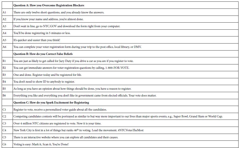
Mind Genomics works by presenting the respondent with specific combinations of messages, viz., so-called ‘elements.’ Step 1 creates these elements. The process begins by the selection of a topic (convincing people to register to vote). The process then proceeds by creating a set of questions which ‘tell a story’, and in turn a set of ‘answers’ or ‘elements’ for each question. In this study, we used a version of Mind Genomics set up for six questions, each question having six answers. The questions are not really questions, per se, but rather what one might call ‘topic sentences’ in writing and rhetoric. They move the account along. Ideally, they should fall into a logical order. Table 1 presents these six questions, and the six answers for each question.

In the Mind Genomics study, the questions are not shown to the respondents. As a result, the answers or elements must ‘stand on their own.’ During the evaluation, the respondent will find it easy to ‘graze’ through the different answers presented in the test combinations and make a judgment. The structure of the question, its clarity, is far less important than the structure of the answer, the element. Ideally, there should be no subordinate clauses, as few connectives as possible, and very little if-then thinking. In other words, simple declarative statements are best.

Table 1: The raw material for the Mind Genomics study, comprising six questions, and six answers (elements) to each question.

table 1(1)

table 1(2)

Step 2: Create Vignettes, the Stimuli to be Evaluated

One of the foundations of Mind Genomics is that the respondents should be required to evaluate vignettes, combinations of elements created according to an underlying experiment design [15]. The experimental design is a set of recipes, in this case 48 different recipes or vignettes for each respondent. Of these, 36 vignettes comprise four elements, with no question contributing more than one element. The remaining 12 vignettes comprise three vignettes, again with no question contribute more than one element. One of the differences between Mind Genomics and conventional research is the way that the underlying patterns are uncovered, viz., in terms of dealing with variability or ‘noise.’ The standard scientific approach is to suppress the noise by doing one element at a time so the respondent can focus on the element, or by testing the same vignette with many respondents, so that the variability can be averaged out. In both cases the research must perforce be limited to the 48 vignettes chosen, so it is good research practice to know a lot about the topic, so that the choice of the elements and the creation of the vignettes is ‘close to as good as it can be.’ The strategy seems adequate, unless of course one does not know much about the answer and does not even know where to start. In such a case, there is a reluctance to spend a lot of money on solid research. The Mind Genomics approach is quite different. The ingoing assumption is that the research should cover as wide a space of alternative combinations as possible, rather than be focused on a small, and presumably promising area. This strategy of covering a wide swath of the ‘design space,’ the world of possible combinations, is accomplished by a permutation strategy [15]. The basic mathematical structure of the experimental design is maintained, but the actual combinations differ. The happy consequence is that each respondent evaluates a different portion of the design space. That is, each respondent evaluates all elements, each element five times in different combinations, but it is the combinations which vary. Only at the end, when the ratings are deconstructed into the contribution of the individual elements do we get a consensus value for each element, the coefficient which is the key to the analysis, the ‘secret sauce’ in the parlance of business.

It is worth noting here that the systematic permutation and the potential for iteration means that the researcher really does not have to know, or even ‘guess’ what are the correct elements, and what are the combinations which will be most productive to reveal the answers to the problems. Rather, the underlying computer program for Mind Genomics will create the combinations for a respondent, present these combinations to the respondent, get the ratings, and store the data. The process is fast, the creation of the different sets of combinations is automatic, built into the system, allowing the entire process, from start to finish, from creating the elements to evaluating the analyzed results, to occur in a matter of hours, or a day at most.

Step 3 – Create the Additional Material for the Study

This material included the orientation page, comprising a short introduction to the topic, as well as a 9-point rating scale. As we see below, the orientation creates very little expectation on the part of the respondent about what the correct answer will be. It will be the task of the elements (Table 1), combined into vignettes (Step 2) which will drive the response. The orientation is simply a way to introduce the respondent to the task. The orientation for this study is simply the question ‘How likely are you to register to vote based on the information above?’. The respondent’s task was simple; read the vignette and rate the vignette. There was not deep information about the need for voting, etc. That information would be provided by the elements. The actual ‘look’ of the question appears below. Note that the vignette occupied the top of the screen, and the rating scale occupied a small section of the bottom of the screen:

box

In addition to the orientation and rating, the respondents were instructed to fill out a short questionnaire on who they were, and gave the researcher the permission to contact them, and to append additional third-party data of a non-confidential source. That additional information augmented the information obtained in the Mind Genomics experiments, allowing the researcher to understand the preferences and way of thinking of individuals based upon WHO they are, and WHAT they do. Such information is the typical type of information served up in studies. By itself the information informs but does not guide directly. Coupled with understand the important elements to drive a person to say she or he will register to vote, the information becomes far more valuable. One can then prescribe, rather than just describe.

Step 4 – Execute the Experiment

The respondents were from New York City participants who were members of a nation-wide panel company, Luc.id. Since around 2010 it has become increasingly obvious that it is virtually impossible to do online research, even with short interviews of more than 30 seconds without compensating the respondent. The days of massive responses to studies are finished, simply because people are both starved for time, and inundated with on-line surveys for every ‘trackable behavior’ of economic relevant. The refusal rate for interviews is skyrocketing. Thus, the use of online panel providers has dramatically increased, removing the onerous tasking of finding respondents for these short studies.

The study encompassed 460 respondents, with an interview lasting about 8-10 minutes. The compensated panelists generally do not ‘drop out’ of the study mid-way, as is the case for unpaid volunteers, where it is difficult to get panelists, and difficult to retain panelists to finish the task.

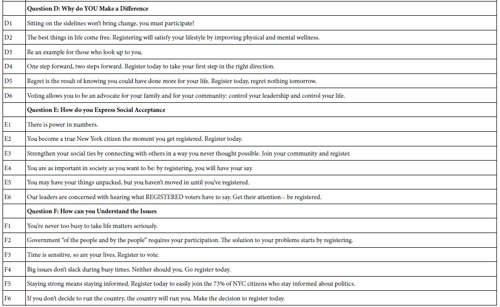
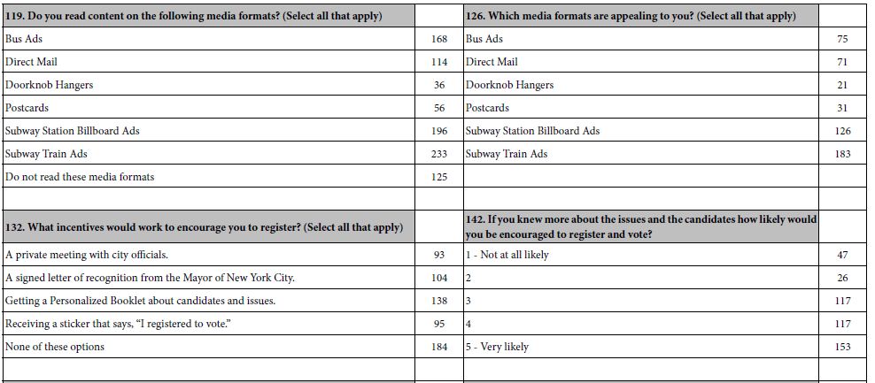
Table 2 gives a sense of the depth of information obtain about each respondent. Some of the questions were asked of the respondent at the time of the interview. Other questions were answered by third-party data purchased for the project.

Table 2: Example of some direct self-profiling classification questions and additional third-party data available and matched to the respondents by matching email addresses. A total of 145 additional data points were ‘matched’ to the study data of each of the 460 respondents.

table 2(1)

table 2(2)

Step 5: Create Models Which Relate the Presence/Absence of the Elements to the Rating

The respondent rated the vignettes on a 9-point scale. One might ordinarily wish to relate the presence/absence of the elements to the 9-point rating. The issue there is that we do not know, intuitively, what a 7 means, or what a 2 means, etc. We do know that the higher numbers mean that the respondent is more likely to register to vote, and that the lower numbers mean that the respondent is less likely to register to vote. That information is directional, but not sufficient.

In consumer and social research circles, there has been a movement to re-code scales such as the 1-9 or similar scales, to make the interpretation easier. We created six new binary scales, as follows:

box 2

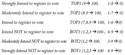
The statistical analysis OLS (ordinary least squares) regression needs some minimum amount of variation in the dependent variable. Across the entire set of 460 respondents, it is very likely that the respondents will not generate the same rating (e.g., TOP3, all respondents rating the 48 respondents 7-9). If the respondents were to somehow do so, the statistical analysis would crash. On the other hand, for individual respondents, it is likely that a respondent might confine all ratings to 1-3, making BOT3 always 100. IN that case, the OLS regression would crash when creating a model or equation for that one respondent, bringing the entire processing to a halt.

To forestall the problem of a ‘crash; we add a vanishingly small number to each of the binary transformed variables that we just create ensuring that the actual transformed ratings vary a very little but do vary around the levels of 0 and 100, respectively. There is no meaningful effect on the regression coefficients emerging after performing this small prophylactic adjustment, but we prevent crashes. Indeed, without this adjustment, about 5% of the respondent models ‘crash’ because the respondent’s transformed numbers either all map to 100 or all map to 0.

The experimental design at the level of both the individual and at the level of the group allows us to create equations relating the presence absence of the elements to the transformed, binary ratings. We create six equations, each expressed as:

Binary Rating = k0 + k1(A1) + k2(A2) … k35(F5) + k36(F6)

Each equation is characterized by its own additive constant, and its own array of 36 coefficients. We interpret the additive constant as the expected percent of the respondents who will register to vote or not register to vote (according to the variable definition), albeit in the absence of elements. The additive constant is a purely estimated parameter but can be used as an index for predilection to register to vote. We expect increasing magnitudes of the additive constant as we go from TOP1 (Definitely intend to register to vote) to TOP3 (Intend to register to vote), and we expect a decreasing magnitude of the additive constant as we go from BOT3 (intend not to register to vote) to BOT1 (definitely not intend to register to vote). For the first analysis, we create six equations or models, based on the data from the total panel, and using each of the newly created binary variables as a dependent variable. With 36 elements, and six dependent variables, the OLS regression generates a massive amount of data (six additive constants, 216 coefficients, viz., 36 coefficients for each of the binary variables). That amount of information overwhelms the researcher, disguising patterns where they exist. To uncover the pattern, we blanked out all coefficients of 3 or lower, only to end with no strong performing elements. For the Total Panel only, we looked at elements with coefficients of +2 or higher. For all other analyses of coefficients, we look at elements with coefficients of +3 or higher. We begin first with the additive constant, the estimated propensity to register to vote, in the absence of elements. As we expected looking for individuals who feel strongly about voting generates a low additive constant of 10 (viz., for TOP1). We are likely to find only about 10% of the responses to be a ‘9’, in the absence of elements. When we make the criterion easier, accepting a 7, 8, or 9, (viz., TOP3) the additive constant jumps to 27.

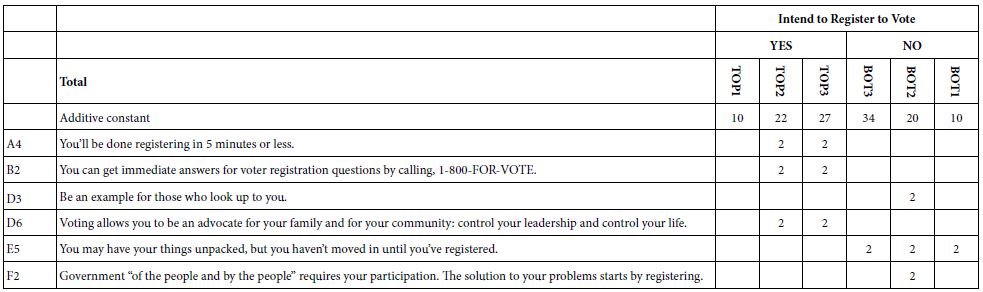
Table 3 shows us that despite our efforts to find motivating elements, only six elements passed the relatively easy screen, viz., a coefficient of +2. The coefficient of +2 is very low in the world of Mind Genomics. Table 3 shows that the effort to find drivers of voting produced only three elements which show any promise, using the data from the total panel, and the promise they show is less than enthusiastic.

A4 You’ll be done registering in 5 minutes or less.

B2 You can get immediate answers for voter registration questions by calling, 1-800-FOR-VOTE.

D6 Voting allows you to be an advocate for your family and for your community: control your leadership and control your life.

When we move to the response ‘Not Register to Vote’ we see a similar pattern. The additive constants are similar in magnitude and go in the right direction. The strong statement about not voting, a rating of 1, captured by the variable BOT1, suggest that 10%, saying they would not definitely register to vote when the criteria are made less strict.

These are the three elements, presumed at the start of the experiment to drive positive voting, but instead drive the opposite, not registering to vote:

D3 Be an example for those who look up to you.

E5 You may have your things unpacked, but you haven’t moved in until you’ve registered.

F2 Government “of the people and by the people” requires your participation. The solution to your problems starts by registering.

Table 3: “Strong’ performing elements from the total panel, defined operationally as a coefficient of at least +2. Only those coefficients are shown. Missing elements failed to generate any coefficients of 2.0 or higher for any of the binary dependent variables.

table 3

Do People Change Their Stated Likelihood of Voting During the Interview?

Having now looked at the data from the total panel, and finding very little, we must pursue the reason why we fail to discover strong elements from the total panel. If we did not have the underlying structure, we would not know how weak the data are from the total panel. We would simply choose the strongest performing vignette and work with that vignette. Such an approach characterizes the research where the stimuli are put together, without structure. If we have one or two or even three or four elements varying, we might make a good guess, but we could not be sure. Mind Genomics take us in a different direction, to uncover the performance of the elements. It is those elements which constitute the building blocks of revised potentially better performing elements. Our first analysis looks at the (possible) change in the rating assigned by the respondents as the interview or experiment progresses. Recall that each respondent evaluated 48 unique vignettes, each vignette comprising 36 combinations of four elements (one from each of four questions), and 12 combinations or vignettes of three elements (one from each of three questions). By design, and by the systematic permutation of the vignettes, respondents saw different vignettes. We cannot measure change in the response to a specified vignette which most likely appeared just a few times, but we can measure the relation (if any) between the average rating assigned by the respondent and the order in the study (rating 1-9 for each vignette, order 1-48).

Our analysis uses OLS regression, done at the level of the individual respondent. For each respondent we know what was assigned to each vignette rated by the respondent, as well as the order of testing. We express the relation as: Rating (9-point scale) = k0 + k1(Order of Testing). The slope, k1, tells us the effect of repeating the interview. We are interested in the sign of the slope, k1, and then the magnitude of the slope. When k1 is positive we conclude that the respondent becomes more interested in registering to vote as the interview or experiment goes on. It may be linked to the respondent being more sensitive to messaging. When k1 is negative we conclude that the respondent becomes less interested in registering to vote as the interview or the experiment on. The respondent may be turned off. In turn, the magnitude of the slope, viz. the numerical value of k1, tells us how many rating points on a 9-point scale will be added to the rating or subtracted from the rating for each additional vignette evaluated. Figure 1 shows the estimated magnitude of change in the rating assigned by a respondent across the 48 vignettes. Most of the respondents show a small change in the rating from vignette #1 to vignette #48. Most the respondents are within +/- two points on the 9-point rating scale. Keep in mind that the regression analysis generating the data was did not look at the actual range, but simply the pattern of changes manifesting itself at the individual respondent level.

fig 1

Figure 1: The distribution of expected ranges to be expected as the respondent proceeds to evaluate 48 vignettes. Most of the range lies between an increase of 2 points to a decrease of 2 points from first vignette to last vignette.

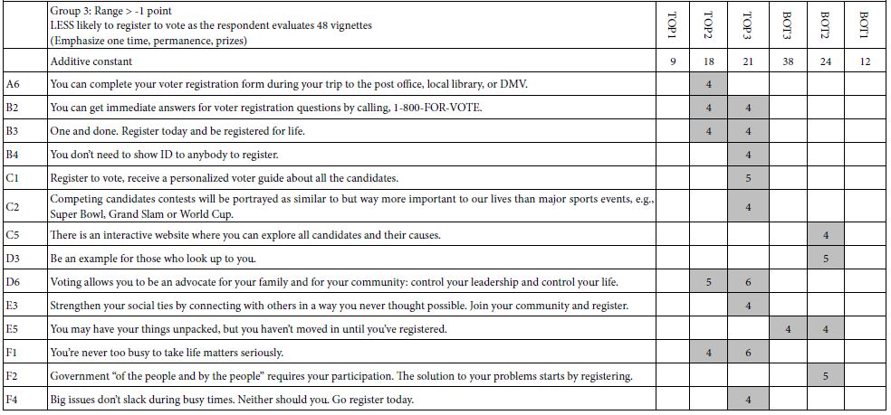
Thus far we know the behavior of the respondent and can differentiate those respondents who are likely to increase versus decrease their ratings. We do not know anything about their criterion for making their judgments. We could ask the respondents to tell us their criteria, but it’s unlikely that they could tell us. The interview is so short, the vignettes judged so quickly, and the attention to the topic only modest while the interview is going on. Despite what might be wished for by novice researchers, most experienced researchers in these types of studies KNOW that their respondents are barely interested in the topic and are answering automatically to stimuli which much seem to them like a ‘blooming, buzzing confusion’. Those are the words of Harvard psychologist William James, when describing how a baby must perceive the world. Fortunately, Step 2 above tells us that despite the response of the respondent (or professional) asked to describe the test stimuli, there is a strongly laid structure underlying each respondent’s set of 48 vignettes. The structure prescribes exactly which elements belong in each vignette, doing so down to the level of a single respondent. We divide the respondents into three groups, defined qualitatively as those with positive range (one point or greater increase in the rating from vignette #1 to vignette #48), those with a flat range (between -1 and +1 point across 48 vignettes), and those with negative range (one point or greater decrease in the rating across 48 vignettes). The first become more interested in registering to vote, the second don’t really change their rating, and the get turned off.

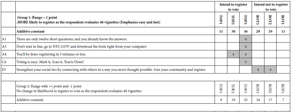
Table 4 shows the strong performing elements for each group. Again, we select only those elements which have a breakthrough coefficient, now defined as +4, but which could easily be changed. The objective is to reduce the ‘wall of numbers’ to a limited set with the patterns coming through.

We see the following patterns emerging:

  1. There are breakthrough elements for Groups 1 (positive range) and Group 3 (negative range), but no strong elements for Group 2 (flat range)
  2. Despite the differences between the groups, and the differences in the patterns of the additive constants, there is no clear ‘story’ about what is driving Group1 (positive range) vs. Group 3 (negative range).

Table 4: Strong performing elements for three groups created on the basis of the range of the 9-point rating to be observed as the respondents proceeds to rate vignette 1 to vignette 48.

table 4(1)

fig 4(2)

We conclude that if there is a story, it is deeper than the observed patterns of responses. Looking at large morphological differences in the patterns of responses gives us a lot of data, a lot of comparisons, but sadly no insight.

Uncovering Underlying Mind-sets based on the Pattern of Coefficients

One of the hallmark features of Mind Genomics is its focus on the decision-making of the everyday, and the recognition that the variability often observed in the data may be result in part from the combination of underlying groups with different criteria. A good metaphor is white light without color. One who looks at white light would say that it is colorless, but the structure of white is that emerges from three primary colors, red, blue, and yellow, respectively. Continuing the metaphor, what if the lack of strong, interpretable patterns in the data come not so much from lack of patterns, nor from intractable variability, but rather from the class of different mind-sets, having different criteria. The failure to uncover strong patterns may be the result of mutual cancellation. Mind Genomics researchers have worked out simple ways to identify these mutually exclusive primary groups, without the benefit of ‘theory’ about how the topic actually works, but simply on the basis of ‘hands-off’, clustering. Recall that each respondent evaluated a unique set of 48 vignettes, embodying the 36 elements in different combinations, with the data from each respondent constituting a complete experimental design. That is, each respondent both evaluated different combinations, but the mathematics of each set of combinations allows us to create a model for that individual [15].

To create these primary groups, or ‘mind-sets’, we followed these steps, adapting the Mind Genomics process, but incorporating two dependent variables simultaneously, register to vote (TOP2), and not register to vote (BOT2).

  1. Create the mind-sets on the basis both of drivers of registering to vote, and drivers of NOT registering to vote. That is, we were interested in moving beyond one direction (drivers of registering to vote)
  2. For each of the 460 respondents, create a model for TOP2 relating the presence/absence of the 36 elements to the TOP2 value. Create another model for BOT2. We thus have 460 pairs of coefficients, each pair comprising 36 coefficients.
  3. When estimating the model for each respondent, do not use the additive constant. The rationale is that we will be combining the two sets of 36 coefficients to create a set of 72 coefficients for each respondent. All the information must be available solely in the coefficients. The technical appendix shows that estimating the coefficients without an additive constant produces the same pattern of coefficients as estimating the coefficients with an additive constant. The only difference is the magnitude of the coefficient. Figure 2 in the Technical Appendix shows the high co-variation between the two sets of coefficients, estimated for the same data, one without and one with the additive constant, respectively.
  4. Create the 460 rows of data, comprising 36 coefficients for TOP2, and 36 coefficients for BOT2. Each respondent now has 72 coefficients.
  5. Use principal components factor analysis to reduce the size of the matrix, by extracting all factors with eigenvalues of 1 or higher. This produced 19 factors.
  6. Rotate the factors by a simplifying method, Quartimax, to produce a set of 19 new factors, rather than 72. Each respondent becomes a set of 19 numbers, the factor scores in the structure, rathe than a set of 72 numbers. We van be sure that the 19 factors are independent of each other.
  7. Extract two and three clusters, or mind-sets, based on strictly numerical criteria [16]. The cluster method is the k means clustering, with the measure of distance between any two people defined by (1-Pearson Correlation between the two people on the 19 factors). In practical terms, any clustering method will do the job, since the clustering is simply a heuristic to divide the 460 respondents into similar-behaving groups
  8. The principal component factor analysis allows us to create models for two segments (mind-sets) corresponding to the two-cluster solution, and three segments (mind-sets) corresponding to the three-cluster solution. The three-cluster solution was clearer. One could extract ore clusters, or mind-sets, but we opted for parsimony.

Create the six equations, with additive constants, for each of the three mind-sets, using the respondents allocated to the mind-sets. Eliminate all elements which fail to exhibit a coefficient of +4 in any model. This step winnows out most of the elements. The elements which remain show strong performance, and also suggest an interpretation, something not seen the previous data because variables did not have ‘cognitive richness’.

Table 5 suggests that there are three subtly different groups

MS 1 – A sense of voting is easy, fun, like sports. Don’t want to be reminded of the ‘seriousness’ of voting

MS 2 – Make it easy, make it simple, learn. They are ready. Nothing really turns them off.

MS 3 – Hates lines, make it easy. That’s all. Avoid talking about social responsibility. It’s a turnoff

The additive constants suggest that Mind-Set 1 (voting as fun) is most likely to register, without messages

Mind-Set 2 is likely to register. Nothing really turns them off.

Mind-Set 3 can be swayed by the right or wrong messages

The three mind-sets differ both in the pattern of likelihood to register and in the topics which turn them off, if there are any. Only Mind-Set 3 really responds in a way that suggest they are turned off.

Table 5: Strong performing elements for three emergent mind-sets (coefficient > = 4).

table 5(1)

table 5(2)
 
fig 2

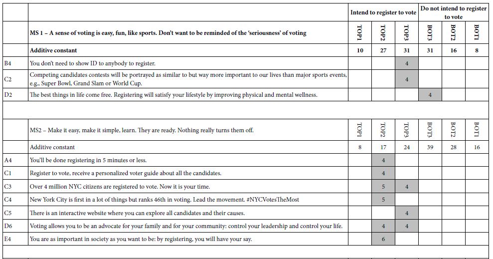
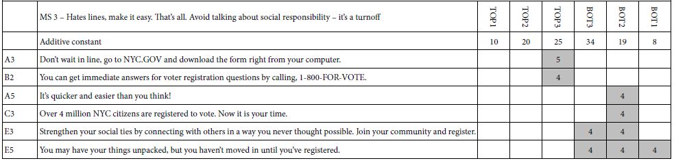
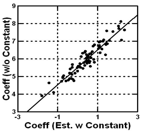
Figure 2: Scatterplot based on the data from the total panel, showing the strong co-variation of the 36 coefficients when estimated with an equation with an additive constant, vs. absent an additive constant.

Synergisms in Messages – Increasing the Likelihood of Mind Set 1 to Say They Will Register to Vote

As noted above, most conjoint measure studies with experimental design focus on a limited set of combinations, with the respondent testing all or only some of the combinations. None of the methods use permuted designs. It is the permuted design which allows the research to explore a great deal of the design space. One of the unexpected benefits is the ability to identify synergism and suppressions between pairs of elements. It to the study of interactions, and the search for synergism that we now turn.

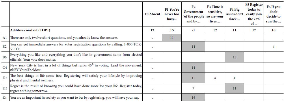
Moskowitz and Gofman [11] introduced the notion of ‘scenario analyses for Mind Genomics. The guiding notion is that pairs of elements may synergize with each other, but the synergy could be washed out in a larger design. A better way to find out whether elements synergize is to select one of the questions (e.g., F), and separate all the data in the study into one of seven different strata, specifically all those vignettes where there is no F (by design), all those vignettes where F is held constant at F1, all those vignettes where F is held constant as F2, etc. Our starting data, therefore, is a set of several strata. We will end up running seven equations of the same type, one equation for each stratum. The equation will have only 30 independent variables (A1-E6), because for each stratus there is a single value of F, a single element. The set of elements from F are no longer independent variables. They simply exist in the vignette, or in the case of F0 deliberately left out of the vignettes. We can now select a target population, e.g., Mind Set 1, and run the regression seven times, once for each stratum. We will choose the most stringent dependent variable, TOP1 (definitely register to vote). The independent variables will be A1-E6, 30 out of the 36 variables. The additive constant is still the expected percent of response TOP1 (rating of 9, definitely register to vote), in the absence of the elements. The coefficients are the incremental percent of responses ‘will register to vote’ when the element appears in the vignette. Armed with that information let us now run the reduced model on each of the seven strata. Table 6 shows the coefficients. The columns correspond to the seven different strata. The rows correspond to the elements which show coefficients of at least +10 in one stratum. These are elements which are expected to synergize. To make navigating easier, and to uncover the strong performing combination, we present only those cells with positive coefficients of +4 or higher. The simplest way to discover combinations is to search for the shaded cells with the highest coefficient and add that high coefficient to the additive constant. The result will be the estimated score for that pair of elements as the key message. There are several very strong combination, combinations that we would not have guessed, first in the absence of mind-set segmentation, and second, in the absence of ability to uncover synergistic (or suppressive) combinations. A good example is the synergistic pair (F4, B6), and then ‘finished off’ with element D5. Table 6 suggests that the total score for TOP1 (definitely would register to vote) would be 11 for the additive constant, 15 for the synergistic pair (F4, B6, or 26 points. There is room for one more element, which we are free to choose, as long as the element makes intuitive sense and fits with F4 and B6. One example could be D5:

F4 = Big issues don’t slack during busy times. Neither should you. Go register today.

B6 = Everything you like and everything you don’t like in government came from elected officials. Your vote does matter.

D5 = Regret is the result of knowing you could have done more for your life. Register today, regret nothing tomorrow.

A possibly better strategy emerges when we look at F2 as an introductory phrase. The element itself does not bode well (additive constant of -1), but it synergizes with four of the six elements show in the stub (row) of Table 6.

F2 Government “of the people and by the people” requires your participation. The solution to your problems starts by registering.

B2 You can get immediate answers for voter registration questions by calling, 1-800-FOR-VOTE.

C4 New York City is first in a lot of things but ranks 46th in voting. Lead the movement. #NYCVotesTheMost

D2The best things in life come free. Registering will satisfy your lifestyle by improving physical and mental wellness.

E4 The best things in life come free. Registering will satisfy your lifestyle by improving physical and mental wellness.

Table 6: Strong pairwise- interactions between elements F1-F6, and the remaining elements. The data come from respondents in Mind-Set 1.

table 6

Discussion and Conclusions

The world of public policy requires that the citizens perform their duties. Some of these duties are mandatory, such as military service, education, and obeying the law. Some are rights, not necessarily duties, such as registering to vote. Ask any group of people about how they feel about registering to vote, and you are likely to get a range of answers, from affirmation of patriotism, to indifference, to the absolute dislike of registering to vote because it is at once disinteresting, a duty, and worst of all, it puts one on the list for jury duty, another public service not in great favor. The sentiments around registering to vote are often simply measured as ‘yes/no’, e.g., will you register to vote or not register to vote. In this Mind Genomics study (really experiment), we have gone into the topic as it were a product or service, being offered to the respondent. We have used the language often used to ‘convince,’ only to discover that across the entire panel respondents, there are really no strong messages. If voting were a service or a product, we would ‘go back to the drawing board’ and try again

The speed, simplicity, cost, and templated structure of Mind Genomics, especially with smaller versions of the study presented here, 16 rather than 36 elements, makes it now possible to iterate through, testing different messages of a ‘public service’ nature. Public service messages may be viewed as a necessary evil, to be checked off, even though they contain little of a sales nature, and are primarily exhortations to do one’s duty and to be good citizens. Or, as Mind Genomics suggest, public service messages may provide the necessary matrix of ideas to use as a way to understand and to motivate the citizen. The study run here itself constitutes a larger-than-usual study in terms of the ideas explored. The results suggest a lack of knowledge of ‘what really motivates people,’ or more correctly a lack of understanding of people who are the targets of communication for a topic which is at best unromantic, quotidian, ordinary, and perhaps even potential negative because it could lead to jury duty. How interesting, however, the study becomes when we peel back the layers, understand the minds of people through segmentation, and through understanding of synergies where two messages combine to do far more than one expected. This type of information, collected across different types of studies, in an iterative process, builds a bank of knowledge for messaging about the common weal, the common good. Having a process such as Mind Genomics embedded in our societal life and in our political process offers far greater benefits to society than we can imagine today. Just imagine messaging for the social good, and doing it expeditiously, inexpensively, effectively.

Technical Appendix Relation between Coefficients Estimated with vs. without the Additive Constant

Mind Genomics is founded on the use of experimental design and OLS (ordinary least-squares) regression. Experimental design creates the test stimuli (vignettes) by specifying the specific combinations. OLS regression deconstructs the response to the vignettes, to estimate the part-worth contribution of each element to the respondent. Traditional Mind Genomics has worked with OLS regressions estimated with an additive constant. The constant is a measure of the likelihood of the response in the absence of the stimulus, a purely theoretical parameter. In this study, comprising six questions, each with six answers or elements, the experimental design called for 48 vignettes. Each element appeared 5x in the 48 vignettes and was absent 43 times. We can estimate two equations for the Total Panel, or indeed two equations for any subgroup, both equations using the same data.

Equation 1: Equation with the additive constant

Binary Dependent Variable (e.g., TOP2) = k0 +k1(A1) + k2(A2) … k36(F6)

Equation 2…which looks exactly like equation 1, but has no additive constant

When we estimate the coefficients, and plot one set against the other in a scatterplot, Figure 2 tells us that the patterns are the same, although the coefficients are higher when there is no additive constant. Figure2 shows an almost perfect co-variation of coefficients estimated in the two ways (R=0.94), with different values, however for the same element.

Acknowledgments

The authors wish to acknowledge the contributions of those students at Pace University, New York, who designed, executed, and wrote up the study for presentation to the Office of the Mayor of New York City. The strategy and messaging were used prior to the elections to encourage New Yorkers to register to vote in the upcoming election. The students then presented the study to professional direct marketers, at a direct marketing conference. In their own words ‘this is a great, practical tool which taught us a lot as we used it and got to see what we could accomplish.’

References

  1. Harder J, Krosnick JA (2008) Why do people vote? A psychological analysis of the causes of voter turnout. Journal of Social Issues 64: 525-549.
  2. Gershtenson J, Plane DL, Scacco, J.M. & Thomas, J., (2013) Registering to vote is easy, right? Active learning and attitudes about voter registration. Journal of Political Science Education 9: 379-402.
  3. Jennings W, Wiezien C (2018) Election polling errors across time and space. Nature Human Behaviour 2: 276-283.
  4. Rubado ME, Jennings JT (2020) Political consequences of the endangered local watchdog: newspaper decline and mayoral elections in the United States. Urban Affairs Review 56: 1327-1356.
  5. Kaufman RR, Haggard S (2019) Democratic decline in the United States: What can we learn from middle-income backsliding? Perspectives on Politics 17: 417-432.
  6. Dale A, Strauss A (2009) Don’t forget to vote: Text message reminders as a mobilization tool. American Journal of Political Science 53: 787-804.
  7. Knack S (1993) The voter participation effects of selecting jurors from registration lists. The Journal of Law and Economics 36: 99-114.
  8. Xu AJ, Wyer Jr RS (2012) The role of bolstering and counterarguing mind-sets in persuasion. Journal of Consumer Research 38: 920-932.
  9. Krantz DH (1964) Conjoint measurement: The Luce-Tukey axiomatization and some extensions. Journal of Mathematical Psychology 1: 248-277.
  10. Green PE, Krieger AM, Wind Y (2001) Thirty years of conjoint analysis: Reflections and prospects. Interfaces 31: S56-S73.
  11. Moskowitz HR, Gofman A (2007) Selling blue elephants: How to make great products that people want before they even know they want them. Pearson Education.
  12. Miller GA, Galanter EH, Pribram KH (2017) (Orig. 1960). Plans and the Structure of Behavior, Routledge.
  13. Moskowitz HR (2012) ‘Mind Genomics’: The experimental, inductive science of the ordinary, and its application to aspects of food and feeding. Physiology & Behavior 107: 606-613.
  14. Moskowitz HR, Gofman A, Beckley J, Ashman H (2006) Founding a new science: Mind Genomics. Journal of Sensory Studies 21: 266-307.
  15. Gofman A, Moskowitz H (2010) Isomorphic permuted experimental designs and their application in conjoint analysis. Journal of Sensory Studies 25: 127-145.
  16. Xu R, Wunsch D (2008) Clustering (Vol. 10). John Wiley & Sons.
Featured Image2

Social Determinants Do Not Determine Me

DOI: 10.31038/AWHC.2021452


The apartment complex in which I lived growing up was called, “The Bellagio,” and its name was written in golden, cursive letters on the exterior of the building. As a child I always thought this name sounded so elegant, like a ballet dance step. But if you unlocked the front door, you would notice the dingy grey carpet, the cracked and yellowing blinds, and the faint stench of tobacco emanating from the apartment of the old man who lived in the unit below. It wasn’t elegant, but to my single mother and me, it was home.

My mother frequently tells me, “I didn’t want us to be another statistic.” What she meant was that as young, Hispanic women who lived below the poverty line, society expected our lives would amount to very little. These multidimensional identities – female, poor, Hispanic – had placed us at the front doorstep of intergenerational poverty, which we would have to defy serious odds to overcome. In medicine, we call these obstacles the “social determinants of health,” which we use to predict and explain health outcomes. But these issues do more than impact risk of disease: they extend their roots into class, career, and community. From the air quality of a neighborhood to the processed sugars in affordable food, they act as the cloudy weather that influences how readily the blossoms of life can bloom. My reflections on my childhood inform my understanding of how these social determinants both did and did not “determine” my life and provide a unique opportunity to serve and advocate for poor families, Hispanic families, and especially those families led by single parents.

Recent data demonstrates that families headed by single mothers are most vulnerable to poverty [1,2] and that their children face greater obstacles related to educational achievement and adjustment in school [3]. Indeed, for many years my mother and I relied on government assistance programs, including Aid to Families with Dependent Children (AFDC), Women, Infants and Children (WIC), and Medicaid, which funded the bare necessities required for child rearing. I remember spending afternoons in a grey government building playing with communal toys that had been well-loved by many children before me while my mother secured diapers and milk for another week.

Despite these barriers, I was fortunate to be among the 6.8% of Hispanic applicants that are accepted to medical school [4,5] a percentage that shrinks even further if you control for class, gender, and single-parent households. This felt strange to me, given that almost 18.5% of the American population is Hispanic or Latino, a number that continues to rise [6]. Together, these statistics suggest a severe underrepresentation of Hispanic medical school applicants and matriculants relative to the age-adjusted US population [5].

I felt the effects of my minority status almost immediately after starting medical school. During my first week, a group of peers were recounting their favorite travel stories. They took turns sharing tales of Icelandic landscapes and tropical paradises. In that moment, I realized I was one of very few to not have had those same kinds of experiences. My only travel history was my semester abroad, and I had taken out extra loans just to afford the plane ticket. It felt like no one else in my medical school cohort had a background like mine. The voice in my head told me that if you’re standing in a space where no one relates to you, that’s an unspoken affirmation that maybe you don’t belong there. This became a pattern, as I was reminded again and again that my peers and I had very different upbringings, leaving me searching for a personal connection to medicine.

Despite these peer interactions that colored my early medical school experience, I found that in clinical practice, many of my patients did share in my life experiences. It felt familiar interacting with patients who lived in poor areas reminiscent of my own neighborhood, or who were children of single parents. These patients remind me that I belong in medicine, and that my visibility and perspective are important. All patients can benefit from encountering physicians that look like them and relate to their background. These relationships can decrease subconscious bias [7], bridge gaps in health care delivery, and build a deeper bond of trust. Interactions with this patient population remind me that I represent the children of poor, Hispanic, single-parent households, and my personal connection to medicine is found in serving them.

One story from my clinical experiences that has remained with me is an encounter I had on the Mother-Baby Unit during my pediatric rotation. We were rounding on a one-day-old Hispanic baby girl whose mother was a single parent. After asking the mother about whether she needed financial assistance, the attending physician handed her a pamphlet on WIC, then wished her a genuine “good luck” before we hurried on to see the next family. As we left, I noticed that the mother had started to cry.

I couldn’t stop thinking about this mom and her child, and how closely this family dynamic mirrored the experience of my own mother. Alone and at the starting line of single parenthood, had someone once handed my mom a pamphlet on WIC? I couldn’t shake the need to go back to her room and take some time to initiate a heartfelt conversation. I rehearsed the different ways I could tell her that I understood her situation first-hand. I wanted her to know that single parenthood didn’t have to define what her and her daughter’s lives could be, and that there was every possibility that her daughter could accomplish anything she wanted, even end up in medical school someday.

As we finished rounding, I walked back to her room and stood outside the door. I started to doubt myself. I wondered if this conversation was inappropriate or unprofessional, or if I was somehow overstepping my boundaries as a medical student. I lingered outside her room for a few minutes, and when I finally walked in, she was asleep. I wish I could say that I came back later, spoke with her, and made a meaningful impact. But instead, I let the fear of repercussions get the best of me. Looking back, that experience taught me that if I want to make a difference in the lives of my patients, I must be brave and bold, as well as confident that these conversations and visibility are needed and necessary.

While I enjoy working with my peers to provide quality care, my sense of community is fulfilled by working with underserved patients. I am motivated to share my stories and explore the ways in which medical professionals can better advocate for and communicate with them. With these efforts, I strengthen my personal value system, bridge gaps in health equity, and pay homage to my upbringing. I am proud to be an example of how although “social determinants” may have an impact on life, they do not automatically determine worth, value, or achievement.

Abbreviations

AFDC: Aid to Families with Dependent Children

WIC: Women, Infants and Children

References

  1. McLanahan S, Percheski C (2008) Family structure and the reproduction of inequalities. Annu Rev Sociol 34: 257-276.
  2. Damaske S, Bratter JL, Frech A (2017) Single mother families and employment, race, and poverty in changing economic times. Social science research 62: 120-133. [crossref]
  3. Carlson MJ, Corcoran ME (2001) Family structure and children’s behavioral and cognitive outcomes. Journal of marriage and family 63: 779-792.
  4. https://www.aamc.org/data-reports/students-residents/interactive-data/2020-facts-applicants-and-matriculants-data Accessed July 19th, 2021.
  5. Lett LA, Murdock HM, Orji WU, Aysola J, Sebro R (2019) Trends in racial/ethnic representation among US medical students. JAMA network open 2: e1910490-e1910490. [crossref]
  6. United States Census Bureau: QuickFacts. 2019. https://www.census.gov/quickfacts/fact/table/US/RHI725219. Accessed June 16th, 2021.
  7. Bean MG, Stone J, Badger TA, Focella ES, Moskowitz GB (2013) Evidence of nonconscious stereotyping of Hispanic patients by nursing and medical students. Nursing research 62: 362-367. [crossref]
photo 1

Hematological Changes Associated with Amoxicillin, Paracetamol and Their Combinations on Rabbits

DOI: 10.31038/IJVB.2021542

Abstract

Extensive use or misuse of antibiotic and analgesic may lead to hematological changes. This study characterized the hematological changes associated with chronic gavage of Amoxicillin and Paracetamol in rabbits.

Amoxicillin, Paracetamol and their combination were dissolved in distilled water and given a rate of (0 mg/kg), (8 mg/kg), (24 mg/kg) and (4 mg/kg+12 mg/kg) to four groups of rabbits (control, amoxicillin, paracetamol and mixture group) respectively for 2 weeks period followed by 6 weeks relaxation period. Then rabbits were authenticated and sacrificed, blood samples were collected in EDTA-containing tubes and analyzed for complete blood counts using the standard blood analysis method.

Results showed significant increase in white blood cell (WBC) count only in paracetamol treatment. Furthermore, significant increases in hemoglobin (HGB), hematocrit (HCT) were observed in all treatments, whereas platelet (PLT) levels significantly increased in amoxicillin and paracetamol treatments and reduced in mixture treatment. In conclusion, the tested compounds significantly changed blood parameters suggesting potential hematotoxicity due to use of amoxicillin, paracetamol or their combination.

Keywords

Amoxicillin, Blood parameters hematotoxicity, Paracetamol

Introduction

Misuse of amoxicillin (an antibiotic) and paracetamol (an analgesic) may become one of the most difficult problems facing the health sector, which must have a quick and effective solution.

Antibiotic are specific chemicals that kill, slow or stop bacterial growth, they are commonly used by physicians to treat bacterial infections. Amoxicillin was first produced in UK in 1970 and used as antibacterial infections for gram positive bacteria [1]. It has a wide spread application for medical treatments [2]. It may cause liver injury [3,4], health risks due to its side effect to many organisms including fish [5,6].

Paracetamol/acetaminophen is one of the most widely used analgesics, clinical studies indicated many side effects [6]. So far, paracetamol or its metabolites may cause severe hepatic failure [7-9], acute live injury and cell death [10,11], inhibition of excessive amount of N-acetyl-p-benzoquinone imine formation [12], binding quinone reductase 2 in the kidney and liver [13] kidney damage [14] and inhibition of mitochondrial respiration [15].

Hematological changes associated with amoxicillin, paracetamol or their combinations among human beings are not fully understood, a gap of information is still missing. The authors designed this study to measure the hematological changes associated with use of amoxicillin, paracetamol and their mixture on rabbits. Rabbits were chosen as experimental animals because they are big enough, and have similar physiology to human beings [16].

Amoxicillin

Amoxicillin is a (2S,5R,6R)-6-[[(2R)-2-Amino-2-(4-hydroxyphenyl)acetyl]amino]-3,3-dimethyl-7oxo-4-thia-1-aza-bicyclo[3.2.0]heptane-2-carboxylic acid, semi-synthetic, acid stable drug belongs to a class of antibiotics called the Penicillins (B-lactam antibiotics).

Materials and Methods

Chemicals

Amoxicillin and Paracetamol (purity 99%) were obtained from Middle East Pharmaceutical and cosmetics laboratories Co .LTD. All other chemicals used in the experiment were purchased from standard commercial suppliers.

Experimental Animals

Adult male rabbits were purchased from locally certified farms. They were housed in a suitable room equipped with air conditioning according to US-EPA 2004 for a period of two weeks initially to acclimate to insure a stable experimental condition. The rabbits were properly maintained according to the principles and guidelines issued by the Ministry of Agriculture in Gaza And US-EPA2004 for animal care, rabbits were individually placed in appropriate steel cages at 22-26°C, 40-70% humidity and a clean environment with a light/12 hour cycle. A suitable diet of balanced feed and clean water has been provided for the duration of the total experiment.

Preparation of Amoxicillin and Paracetamol Solution

One gram (1000 mg) of Amoxicillin was dissolved in 100 ml of distilled water and1000 mg of Paracetamol was dissolved in 100 ml of distilled water under magnetic steering to ensure complete solubility of drugs . This was visualized by clean solution of water.

Experimental Design

Rabbits were randomly subdivided into four groups five rabbits each group, and monitored during 10 weeks, study period, (2 weeks of acclimatization +2 weeks of treatment +6 weeks without treatment). After acclimatization period, rabbits received the following treatments:

Group 1: Each rabbit received by oral administration amoxicillin at a rate of 8 mg/kg BW for 14 days; Group 2: Each rabbit received by oral administration paracetamol dose at a rate of 24 mg/kg BW for 14 days; Group 3: Each rabbit received by oral administration a mixture of Amoxicillin and paracetamol at a rate of 4 mg/kg BW+12 mg/kg BW for 14 days; and Group 4: control group, each rabbit received by oral administration 1 ml distilled water/rabbit for 14 day. Photo 1 shows the gavage process of the tested compounds.
photo 1

Photo 1: Oral administration of the tested compounds on rabbits

Collection of Blood Samples

At the end of the experimental period (10 weeks) rabbits were authenticated to for blood sample collections via cardiac puncture into sterile tubes containing EDTA to prevent blood clotting, then analyzed for CBC using standard method and previously described [17].

Statistical Analysis

Average and standard deviation were calculated. Analysis of Variances (ANOVA) was employed to detect significant differences among treatments at p-value 0.05. p-value ≤ 0.05 indicates significant differences among treatments whereas values > 0.05 are not significant.

Results

Effects on the Blood

Effects of the tested compounds on white blood cells (WBC) are shown in Figure 1.

fig 1

Figure 1: Chemical structure of amoxicillin and paracetamol.

It can be seen that concentration of WBC was increased in the treated rabbits above that of the control group. Statistical analysis detected significant differences only in paracetamol treatment.

Effects on blood lymph (LYM) are shown in Figure 2.

fig 2

Figure 2: Concentrations of WBC in rabbit treated with Amoxicillin, Paracetamol, and their mixture. Error bars represent standard deviation. Columns have the same letter are not significantly different at p ≤ 0.05.

Similarly, to the effects on WBC (Figure 2) increased levels of LYM were observed in rabbits treated with the tested compounds but statistical analysis did not detect significant differences among treatments.

Effects of the tested compounds on red blood cells are shown in Figure 4. Similarly, to the effects on lymph, increased level of red blood cells were observed in the treated rabbits but no significant differences were detected.

fig 4

Figure 4: Concentrations of RBC in rabbit treated with Amoxicillin, Paracetamol, and Their mixture. Error bars represent standard deviation.
Columns have the same letter are not significantly different at p ≤ 0.05.

Effects of the tested compounds on the blood hemoglbine (HGB) are shown in Figure 5. Increased levels of HGB were observed in the treated rabbits. Satstical analysis detected significant difference among all treatment. this suggests an occurrence different biochemical reactions between HGB and the tested compounds.
fig 5

Figure 5: Concentrations of HGB in rabbit treated with Amoxicillin, Paracetamol, and Their mixture. Error bars represent standard deviation.
Columns have the same letter are not significantly different at p ≤ 0.05.

Effects of the tested compounds on hematocreate (HCT) are shown in Figure 6. Similarly to the above effects, increased level of HCT were found in the treated rabbits but statistical differences were detected only in Amoxicillin and mixture treatments.
fig 6

Figure 6: Concentrations of HCT in rabbit treated with Amoxicillin, Paracetamol, and Their mixture. Error bars represent standard deviation.
Columns have the same letter are not significantly different at p ≤ 0.05.

Effects of the tested compounds on the platlets (PLT) are shown in Figure 7. Similarly to the above effects, increased level of PLT were found in the treated rabbits. Statistical analysis detected significan differences.
fig 7

Figure 7: Concentrations of PLT in rabbit treated with Amoxicillin, Paracetamol, and Their mixture .Error bars represent standard deviation.
Columns have the same letter are not significantly different at p ≤ 0.05.

The concentration of WBC and PLT in rabbits blood treated with Paracetamol were the highest among all treatments then Amoxicillin, whereas the concentration in rabbits treated with Mixture were lower than those of the control samples.

Discussion

Amoxicillin used as an antibiotic against bacteria [18] whereas paracetamol used as an analgesic for many diseases. There usage was associated with many complications as mentioned above. Furthermore, their chemical structure (Figure 1) shows the presence of highly water soluble groups such as (OH; C=O) which facilitate interaction and movement of the compounds in aqueous phase such as blood system. Additionally, the chemical structure includes phenyl ring which may enable covalent bonding with liver, kidney, and/or other tissue causing induced injury, in accordance with Lee et al. [19] who revealed similar phenomenon with other cases. Photo 1 show the oral gavage process of the tested compounds. The data in Figure 2, clearly demonstrates the effects of tested compounds on WBC. It can be seen that Amoxicillin and paracetamol increased WBC above that of the control, whereas the combination reduced the values. This suggests that treatments with Amoxicillin and paracetamol enhance the immune system to produce more WBC to defend the body from amoxicillin and paracetamol. Thus an increase of WBC cell would have occurred to enrich the body with the required level of WBC to insure health body. Our explanation agree with Díaz et al., [20] and Zarkesh et al., [16] who revealed the importance of WBC count on blood levels as long as the body exposed to bacterial infections and/or toxic chemicals [21,22].

On the other hand, the combination of the compounds did not increase the WBC. This suggests that the amoxicillin and paracetamol may antagonize each other in the combination accordingly no increase in WBC was observed (Figure 2). Furthermore, it can be suggested that application of the compounds in combination may provide a protection against possible injury. This suggestion is in agreement with [9] who revealed the activity of chiisanoside against liver injury induced by paracetamol in mice.

Nevertheless, the data in Figure 3, clearly shows increased levels of LYM but they remained insignificant with the control sample. This suggests that LYM does not involve in the immune system in the body. Similarly, no significant effects on RBC (Figure 4). This indicates that RBC is not involved in the immune system. On the other hands, HGB levels (Figure 5) are significantly increased in the treated rabbits. This suggests that HGB is involved in the defense systems throughout antibody antigen reactions. Our results are in accordance with El Menyiy et al. [23] and Biu et al. [24] who found that paracetamol significantly increased hemoglobin and platelet count as compared to the control group. An explanation of these results is that amoxicillin and paracetamol caused a dehydration process to the tested animal (data not shown) which may result in a hem concentration. Additionally, it can be suggested that paracetamol and/or amoxicillin can directly interact with blood system to further enhance the production of hemoglobin. Furthermore, it was reported that Paracetamol bond quinone reductase 2 in liver and kidney which modulated reactive oxygen species generation. This may further enhance the toxicity of paracetamol via quinone reductase 2 mediated superoxide production [13].
fig 3

Figure 3: Concentrations of LYM in rabbit treated with Amoxicillin, Paracetamol, and Their mixture. Error bars represent standard deviation.
Columns have the same letter are not significantly different at p ≤ 0.05.

So far, lack of hemoglobin due to paracetamol or amoxicillin exposure may enhance the body to produce more hemoglobin to compensate the losses consequently an increase in hemoglobin level may be observed. Furthermore, the tested compound may cause hematotoxicity by restoring almost normal counts of the hematological parameters through oxidative stress. Our explanation agrees with Oyedeji et al. [25] who report oxidative stress in rat experiments. Influence of the tested compounds on HCT (Figure 6) showed significant increase in the treatment of Amoxicillin and mixture. The explanation on these results is similar to that given above for HGB. On the other hands significant increases in PLT levels (Figure 7) were observed in all treatments. An explanation of these results is that the tested compounds directly interact with PLT counts resulting in either activation as in amoxicillin and paracetamol or aggregation phenomenon as in mixture. Thus PLT tends to increase or decrease (Figure 7). Our explanation is in accordance with Siauw et al. [26] who provided evidence of the direct involvement of platelets with bacterial toxins.

Mode of Interactions

It can be suggested that amoxicillin and/or paracetamol be oxidized by dehydrogenase enzymes in human or animal body producing oxygen reactive species (ORS) as shown in Figure 8. Then these ORS react with blood systems resulting in elevation of HGB, HCT, and PLT in case of amoxicillin and WBC and PLT in case of paracetamol.
fig 8

Figure 8: Possible mode of action of amoxicillin (A) and paracetamol (B) on blood systems after oxidation by dehydrogenase enzyme.

Moreover, the antagonistic effects of amoxicillin and paracetamol in the combination may result from the fact that both molecules have some similarity in the chemical structure such as phenyl ring, C=O, NH2, CH3, OH,. This similarity enhance hydrogen bonding, hydrophobic interactions and possible covalent bonding between both molecule resulting in a larger size molecule than parent ones (paracetamol, amoxicillin). This molecule can move freely in the human body and may not be able to be oxidized by dehydrogenases consequently no ORS were produced. Accordingly, WBC, HGB, LPT HCT contents remained in the acceptable range. This explanation is in accordance with El-Nahhal [27] who revealed hydrogen bonding and hydrophobic interactions between an organic molecules and acetylcholine esterase in human blood. Furthermore, previous reports [28,29] revealed the solubility of similar organic molecules to each other in aqueous solution. Similar observations were recently reported with other cases [30-34]. Additionally, our results are in accordance with Mwafy and Afana who revealed changes in hematological parameters, serum iron and vitamin B12 levels in hospitalized Palestinian adult patients treated with amoxicillin.

Conclusion

The rational of this work emerged from the fact that paracetamol and amoxicillin are widely used pharmaceuticals and their hematological effects are poorly investigated. Elevation of WBC, HGB, LPT HCT levels in treated rabbits were significantly increased indicating high potential of hematological changes. Amoxicillin has a tremendous effect on blood components more that paracetamol has. Combination of both molecules did not produce significant changes on blood parameters indicating a possible protection to blood components. An interesting outcome of the study is that combination of both molecules can be a safe administration for this case.

References

  1. Kaur SP, Rao R, Nanda S (2011) Amoxicillin: a broad spectrum antibiotic. Int J Pharm Pharm Sci 3: 30-37.
  2. Tong DC, Rothwell BR (2000) Antibiotic prophylaxis in dentistry: a review and practice recommendations. The Journal of the American Dental Association 131: 366-374. [crossref]
  3. Abenavoli L, Libri E, Bosco D, Gallo D, Luzza F (2012) Drug-induced liver Recenti Prog Med 103: 79-84. [crossref]
  4. Nicoletti P, Aithal GP, Bjornsson ES, Andrade RJ, Sawle A, et al. (2017) Association of Liver Injury From Specific Drugs, or Groups of Drugs, With Polymorphisms in HLA and Other Genes in a Genome-Wide Association Study. Gastroenterology 152: 1078-1089. [crossref]
  5. Elizalde-Velázquez A, Martínez-Rodríguez H, Galar-Martínez M, Dublán-García O, Islas-Flores H, et al. (2017) Effect of amoxicillin exposure on brain, gill, liver, and kidney of common carp (Cyprinus carpio): The role of amoxicilloic acid. Environ Toxicol 32: 1102-1120. [crossref]
  6. Jóźwiak-Bebenista M, Nowak J Z (2014) Paracetamol: mechanism of action, applications and safety concern. Acta poloniae pharmaceutica 71: 11-23. [crossref]
  7. Hinson JA, Roberts DW, James LP (2010) Mechanisms of acetaminopheninduced liver necrosis. Handb Exp Pharmacol 196: 369-405. [crossref]
  8. James LP, McCullough SS, Knight TR, Jaeschke H, Hinson JA (2003) Acetaminophen toxicity in mice lacking NADPH oxidase activity: role of peroxynitrite formation and mitochondrial oxidant stress Free. Radic Res 37: 1289-97. [crossref]
  9. Bian X, Wang S, Liu J, Zhao Y, Li H, et al. (2018) Hepatoprotective effect of chiisanoside against acetaminophen-induced acute liver injury in mice. Nat Prod Res 15: 1-4. [crossref]
  10. deLemos AS, Ghabril M, Rockey DC, Gu J, Barnhart HX, et al. (2016) Drug-Induced Liver Injury Network (DILIN) Amoxicillin-Clavulanate-Induced Liver Injury. Dig Dis Sci 61: 2406-2416. [crossref]
  11. Cao P, Sun J, Sullivan MA, Huang X, Wang H, et al. (2018) Angelica sinensis polysaccharide protects against acetaminophen-induced acute liver injury and cell death by suppressing oxidative stress and hepatic apoptosis in vivo and in vitro. Int J Biol Macromol 111: 1133-1139. [crossref]
  12. Bajt ML, Knight TR, Lemasters JJ, Jaeschke H (2004) Acetaminopheninduced oxidant stress and cell injury in cultured mouse hepatocytes: protection by N-acetyl cysteine. Toxicol Sci 80: 343-9. [crossref]
  13. Miettinen TP, Björklund M (2014) NQO2 is a reactive oxygen species generating off-target for acetaminophen. Mol Pharm 11: 4395-404. [crossref]
  14. Ghosh J, Das J, Manna P, Sil PC (2010) Acetaminophen induced renal injury via oxidative stress and TNF-alpha production: therapeutic potential of arjunolic acid. Toxicology 268: 8-18. [crossref]
  15. Satav JG, Bhattacharya RK (1997) Respiratory functions in kidney mitochondria following paracetamol administration to young-adult and old rats. Indian J Med Res 105: 131-5. [crossref]
  16. Zarkesh M, Sedaghat F, Heidarzadeh A, Tabrizi M, Bolooki-Moghadam K, et al. (2015) Diagnostic value of IL-6, CRP, WBC, and absolute neutrophil count to predict serious bacterial infection in febrile infants. Acta Med Iran 53: 408-11. [crossref]
  17. El-Nahhal Y, Al_shareef A (2018) Effective biomarkers for successful management of sepsis. Trends in Medicine 18: 1-8.
  18. Kim BJ, Kim JG (2013) Substitutions in penicillin-binding protein 1 in amoxicillin-resistant Helicobacter pylori strains isolated from Korean patients. Gut Liver 7: 655-660.
  19. Lee J, Ji SC, Kim B, Yi S, Shin KH, et al. (2017) Exploration of Biomarkers for Amoxicillin/Clavulanate-Induced Liver Injury: Multi-Omics Approaches. Clin Transl Sci 10: 163-171. [crossref]
  20. Díaz MG, García RP, Gamero DB, González-Tomé MI, Romero PC, et al. (2016) Lack of Accuracy of Biomarkers and Physical Examination to Detect Bacterial Infection in Febrile Infants. Pediatr Emerg Care 32: 664-668. [crossref]
  21. El-Nahhal Y (2017) Risk Factors among Greenhouse Farmers in Gaza Strip. Occupational Diseases and Environmental Medicine.
  22. El-Nahhal Y, Lubbad R (2018) Acute and single repeated dose effects of low concentrations of chlorpyrifos, diuron, and their combination on chicken. Environmental Science and Pollution Research.
  23. El Menyiy N, Al-Waili N, El Ghouizi1 A, Al-Waili W, Lyoussi B (2018) Evaluation of antiproteinuric and hepato-renal protective activities of propolis in paracetamol toxicity in rats. Nutrition Research and Practice 12: 535-540. [crossref]
  24. Biu AA, Yusufu SD, Rabo JS (2009) Studies on the effects of aqueous leaf extracts of Neem (Azadirachta indica A juss) on haematological parameters in chicken. Afr Sci 10: 189-92.
  25. Oyedeji KO, Bolarinwa A, Ojeniran SS (2013) Effect of paracetamol (acetaminophen) on haematological and reproductive parameters in male albino rats IOSR. J Pharm Biol Sci 4: 65-70.
  26. Siauw C, Kobsar A, Dornieden C, Beyrich C, Schinke B, et al (2006) Group B streptococcus isolates from septic patients and healthy carriers differentially activate platelet signaling cascades. Thromb Haemost 95: 836-849. [crossref]
  27. El-Nahhal Y (2018) Accidental Zinc Phosphide Poisoning among Population: A Case Report. Occupational Diseases and Environmental Medicine 6: 37-49.
  28. El-Nahhal Y, Safi J (2004) Adsorption behavior of phenanthrene on organoclays under different salinity levels. Journal of Colloid and Interface Science 269: 265-273.
  29. El-Nahhal Y, Safi, J (2004) Stability of an organo clay complex: effects of high concentrations of sodium chloride. Applied Clay Science 24: 129-136.
  30. El-Nahhal Y, Raaed Lubbad, Mohammad R Al-Agha (2020) Toxicity Evaluation of Chlorpyrifos and Diuron below Maximum Residue Limits in Rabbits Toxicology and Environmental Health Sciences.
  31. Matozzo V, Battistara M, Marisa I, Bertin V, Orsetti A (2016) Assessing the Effects of Amoxicillin on Antioxidant Enzyme Activities, Lipid Peroxidation and Protein Carbonyl Content in the Clam Ruditapes philippinarum and the Mussel Mytilus galloprovincialis Environ Contam Toxicol 97: 521-7. [crossref]
  32. Mwafy SN, Afana WM (2018) Hematological parameters, serum iron and vitamin B12 levels in hospitalized Palestinian adult patients infected with Helicobacter pylori: a case-control study. Hematol Transfus Cell Ther 40: 160-165. [crossref]
  33. Mihalaş E, Matricala L, Chelmuş A, Gheţu N, Petcu A, et al. (2016) The Role of Chronic Exposure to Amoxicillin/Clavulanic Acid on the Developmental Enamel Defects in Mice. Toxicol Pathol 44: 61-70. [crossref]
  34. Seal P, Sikdar J, Roy A, Haldar R (2017) Acetaminophen interacts with Human Hemoglobin: Optical, Physical and Molecular modeling studies. J Biomol Struct Dyn 35: 1307-1321. [crossref]
fig 2

Acupuncture Emergency Service in Brazilian Public Health System: Quantitative Analysis of Cases Attended in a Semester

DOI: 10.31038/PEP.2021247

Abstract

Background: Acupuncture is an effective technique for pain relief and is usually practiced in outpatient clinic setting. It can also be applied in emergency setting focusing on pain relief from non-life threatening diseases.

Objectives: This quantitative, retrospective and descriptive study aimed to demonstrate the dynamics of the Acupuncture Emergency Service at Hospital São Paulo (AES-HSP), linked to the Paulista School de Medicine of the Federal University of São Paulo (Escola Paulista de Medicina – EPM / UNIFESP), which provides free care for the population since 1998.

Methods: Data were collected from the care records of the second half of 2019, assessing gender, age group, complaint, technique (s) used, percentage of improvement reported by the patient and Visual Analogue Scale before (VASb) and after treatment (VASa).

Results: We identified 7647 visits, of which 78.3% (n=5986) were female; the mean age was 60.8 ± 14.3 years-old; the most common complaints were low back pain (26.4%), followed by shoulder pain (17.5%) and knee pain (14.8%); systemic acupuncture was used in a total of 7032 cases, only acupuncture microsystems were used in 615 cases, microsystems and systemic acupuncture were combined in 1815 cases; VASb average was 6.29 ± 2.17, while VASa average was 1.44 ± 1.42; in 21.4% of 6423 visits properly registered, patients reported 100% improvement and 72.2% reported more than 50% improvement.

Conclusion: Our service provides effective pain relief, allowing to receive a great demand from patients with fast execution in an emergency setting, reducing the use of pain killers and its side effects.

Keywords

Acupuncture analgesia, Traditional Chinese Medicine, Public health, Pain Control

Introduction

Musculoskeletal pain (MSP) is classified as acute or chronic, and is the most prevalent symptom in the world population. Its prevalence has increased in recent years due to higher prevalence of risk factors related to lifestyle habits, such as smoking, anxiety, physical inactivity, sleep disorders. Additional influences include low educational level, precarious family income and social isolation [1,2]. In addition, MSP represents an important cause of morbidity, with a large impact on quality of life and in the economic sphere, for example, absence from work, sometimes requiring long periods of recovery [3].

European data related that 15-20% of primary health care appointments are due to musculoskeletal problems [4].

In Brazil, a meta-analysis performed in 2012 estimated the prevalence of chronic MSP ranging from 14.1-85.5%. Considering only Brazilian studies were evaluated in the meta-analysis, the most affected sites were the dorsal spine and the lower limbs [5].

The impact of chronic pain on national economy also reaches a large proportion. For example, in 2007, Australia, a country with approximately 22.7 million inhabitants, had an estimated cost of $34.3 billion for expenses related to chronic pain, with an average of $10,847 per person with chronic pain [6].

The western medicine approach to MSP is mainly based on the use of common analgesics, opioids, anti-inflammatories and physical therapy. Allopathic drugs, however, are not exempt from adverse effects [7]. In addition, the presence of comorbidities, such as high blood pressure, diabetes, and chronic kidney disease, may restrict the use of such medications. Moreover, the inadequate follow-up of prescriptions and the practice of self-medication predispose to the overuse of anti-inflammatory drugs, which may cause serious complications, such as acute renal dysfunction, upper gastrointestinal bleeding due to peptic ulcer disease and occurrence of cardiovascular events [8-10]. The excessive use of opioids, in turn, might result in an increasing number of drug overdose, addiction and deaths [7].

Acupuncture has an energetic propaedeutic role, capable of detecting and treating an individual’s imbalances before they evolve into organic diseases. In addition to the preventive aspect, it is an effective and safe therapeutic tool for many diseases [11].

The mechanism of action of acupuncture involves stimulation of peripheral nociceptors at specific points, which reach the nervous system through neuronal pathways. Neuromodulation occurs at three levels: local, spinal and supraspinatus, resulting in the release of different substances, such as neurotransmitters, that modulate motor, sensory, autonomic, neuroendocrine and emotional responses [12]. Is important to achieve the Te Qi needling sensation, characterized as a set of sensations, such as pain, burning, tingling, pressure, weight, anesthesia and/or shock, directly related to clinical efficacy [13].

In the west, the growing demand for acupuncture treatment is due to its effectiveness in pain complaints, especially in individuals with limitations to traditional pharmacological treatment [14].

In Brazil, the practice of acupuncture was introduced for the first time in SUS in 1999, through Ordinance No. 1230/GM [15], and was reinforced by its inclusion in the National Policy of Integrative and Complementary Practices (PNPIC), published in Ministerial Ordinance No. 971 of May 2006 [15].

In 1992, the Chinese Medicine-Acupuncture Group of the Department of Orthopedics and Traumatology at Paulista School of Medicine of Federal University of São Paulo (EPM/UNIFESP) was created by Ysao Yamamura M.D., PhD. This physician established this group to foment academic undergraduate and graduate activities, including clinical research, of the institution.

Initially, the therapeutic proposals were exclusively provided on an outpatient basis, resulting in great demand by the population, with an average number of 90 patients daily. Due to increasing demand, it was necessary to establish a more dynamic service. The AES-HSP, characterized by providing public assistance predominantly focused on analgesia under free demand access, was opened in 1998.

The AES-HSP team is composed of resident physicians, preceptors, graduate students and interns in the Chinese Medicine-Acupuncture Group. We have four patient care rooms in the outpatient clinic building of Hospital São Paulo (HSP), located in the Vila Clementino neighborhood in the city of São Paulo, state of São Paulo, Brazil. Clinic is held Monday to Friday from 8 am-3 pm, except on holidays. Patients are referred by basic health units or present directly; they are attended to based on arrival order.

In our service, a minimum number of acupuncture points with immediate effect of analgesia is used, with emphasis on the Yamamura System techniques of Acupuncture (SYA/EPM).

Microsystems, or somatotopies, are representations of the entire organism in smaller areas of the body. When the organism is sick, reactive points emerge in the microsystem in the areas corresponding to the compromised region. Through the manipulation of these reflex points, it is possible to act positively on the disease or symptomatology in question. In our service, we use internationally-renowned techniques, such as Yamamoto New Scalp Acupuncture (YNSA), Chinese Scalp Acupuncture and Chinese Auriculotherapy, as well as exclusive techniques developed by Dr. Yamamura [16-18] including the Yamamura Nasal Bone Acupuncture System (Figure 1), Yamamura Acupuncture System Hair Implantation (SYALIC) (Figure 2), Yamamura Long Bone Acupuncture System (SYAOL) (Figure 3), Yamamura Occipital Bone Acupuncture System (Figure 4), Yamamura System of Cranial Sutures and 5 Zang in parietal suture (Figure 5). Some of the main techniques are described below, and may be used isolated or associated with systemic acupuncture. Image of the systems of the Yamamura Acupuncture System were kindly provided by Dr. Yamamura.

fig 1

Figure 1: Yamamura acupuncture system of nasal bone.

fig 2

Figure 2: SYALIC – Yamamura acupuncture system of hair implantation line.

fig 3

Figure 3: Yamamura acupuncture system of cranial sutures and 5 Zang on squamous suture.

fig 4

Figure 4: Yamamura acupuncture system of occipital bone.

fig 5

Figure 5: SYAOL – Yamamura acupuncture system of Long bone.

Methods

We collected data from the attendance records at the AES-HSP, between July-December 2019, using a standardized form completed by the attending physician. The parameters evaluated included gender, age group, complaint, technique(s) used, percentage of improvement reported by the patient and Visual Analogue Scale before treatment (VASb) and after treatment (VASa).

We considered the total number of visits, not discriminating whether the same patient was seen on more than one occasion, and the main and associated complaints. Regarding treatment, we grouped the different approaches into isolated systemic therapy, non-systemic techniques or a combination of both.

A focused anamnesis and physical examination was performed for each patient and was directed to the patient’s complaint in order to correctly select treatment points and techniques. Local asepsis was performed with cotton soaked in 70% alcohol, and sterile, disposable, 0.30 mm x 40 mm stainless steel acupuncture needles supplied by HSP were used. Needle insertion at specific points was performed until the Te Qi sensation was obtained, according to the depth characteristics. In auricular acupuncture, we used mustard seeds affixed to tape and manipulated with the aid of surgical tweezers.

Statistical analysis was performed descriptively, denoting average, median, minimum and maximum values, standard deviation, absolute and relative frequencies in percentage (%), using Microsoft Excel® 2019 software by Microsoft. The graphs of columns and lines were elaborated using Microsoft PowerPoint® 2019 software by Microsoft.

Results

We identified 7,647 visits, of which 78.3% (n=5986) were female and 21.7% (n=1661) were male. Regarding the age group, the mean age was (mean ± standard deviation) 60.8 ± 14.3 years, with a median of 64 years; 85.7% of participants were between 41-80 years (Graph 1), with a predominance in the range of 61-80 years, with a value of 53.4%. The average number of visits corrected for working days in the semester (120) was 63.7 visits/day. The average number of patients per operating time (7 hours) was approximately 9.1 patients/hour, resulting in a duration of care of approximately 6.5 minutes/patient.

graph 1

Graph 1: Distribution by age group (%) (n=7647).

Regarding complaints, low back pain (26.4%), followed by shoulder pain (17.5%), knee pain (14.8%), neck pain (11.7%), upper back pain (5.9%), lower limb pain (5.4%), upper limb pain (4.9%), foot pain (4.9%), polyarthralgia (4.3%), hip pain (2.7%), polymyalgia (2.3%), wrist pain (1.3%), non-restorative sleep (1.3%), hand pain (0.9%), finger pain (0.7%), facial palsy (0.7%) and ankle pain (0.5%). This data is depicted in Graph 2.

graph 2

Graph 2: Percentage of most prevalent pain sites.

In the analysis of the VAS, the data referring to the index in VASb (n=4080 visits) corresponds to an average of 6.29, with a median of 6 and standard deviation of 2.17. For the index in VASa (n=3913), there was an average of 1.44, median of 1 and standard deviation of 1.42. There was a failure to register 46.6% (n=3567) of the VAS in relation to the total number of cases in the semester. The total visits (n=6423) analyzed from the perspective of the degree of response to the treatment perceived by the patient were grouped into five categories: worsening (0%), without improvement (2%), less than 50% improvement (4.3%), more than 50% improvement (72.2%) and 100% improvement (21.4%). This information is presented in Graphs 3 and 4.

graph 3

Graph 3: VAS before treatment (VASb) and after treatment (VASa).

graph 4

Graph 4: Continuous comparison of pain level before treatment (VASb) and after treatment (VASa).

Considering the total number of visits, non-systemic techniques were used 2,430 times. These techniques included: the Bregma craniometric point (22.2%), Anatomical Trains (14.6%), Auriculotherapy (13.2%), Yamamoto New Scalp Acupuncture-YNSA (12.1%), Pterion craniometric point (9.1%), Symmetry (7.8%), Lambda Craniometric point (6.7%), Asterion craniometric point (4.6%), 5 Zang in parietal suture (2.8%), Yamamura Acupuncture System Hair Implantation-SYALIC (1.7%), Yamamura Long Bone Acupuncture System-SYAOL (0.8%), Yamamura Occipital Bone Acupuncture System (0.5%), Yamamura Nasal Bone Acupuncture System ( 0.4%), Yamamura Acupuncture System of the Musculoskeletal System of Sutures (0.4%), Vertebral Points (0.3%), and Chinese Scalp Acupuncture (0.1%) [15-17]. Graph 5 depicts this information.
graph 5

Graph 5: Distribution of non-systemic techniques most used (n=2430).

Systemic acupuncture techniques were used in 7,032 cases, corresponding to 91.9% of total cases. The use of non-systemic techniques alone occurred in 615 cases, corresponding to 8% of the total. Microsystems and systemic acupuncture were combined in 1815 cases (23.7%).

Discussion

Our study identified a female prevalence rate three times higher than males. This information is in agreement with other studies, which state that the prevalence of women reporting chronic pain is generally higher than men, which can be influenced by the way men and women experience pain [19]. Another possible explanation is the social expression of each gender. Women are usually taught to express emotions and seek help, while men are generally inhibited from expressing themselves [20]. Thus, male patients are less likely to report chronic pain and seek medical assistance.

When we analyzed age group, we found that more than half of patients were between 41-80 years of age. According to the literature, older patients have a higher prevalence of chronic pain than younger patients. This may result from the increase in number of comorbidities presented in the elderly [21].

According to the Global Burden of Disease Study in 2016, low back pain and neck pain are the main causes related to disability worldwide [22]. Another study highlights low back pain as the main cause of disability globally [23]. The present study is in agreement with this worldwide incidence since the most frequent complaint was low back pain. Regarding shoulder pain, we found involvement in 17.5% of individuals. This data differs from the Brazilian meta-analysis by Miranda et al. (2012) that assessed the prevalence of musculoskeletal disorders in the elderly population in Brazil and found the spine as the most affected location and the lower limb the second-most affected [5]. Chronic knee pain presented as an important highlight in the visits, since it was the third most prevalent complaint.

Patients suffering from chronic pain often have more than one affected site, as demonstrated in a British demographic survey, in which only one-third of the participants with pain had localized symptoms [2]. Thus, in the prevalence chart of the most frequent complaints, the statistics of different sites of pain must be interpreted separately, only in relation to the total number of cases once the sum of painful sites exceeds the number of visits, because patients usually had more than one complaint.

The VAS was chosen to assess the degree of pain before (VASb) and after (VASa) the treatment with acupuncture because it is a validated instrument of easy applicability and reproducibility, low cost, and widely used in global literature, which allows comparison of the results [24,25]. Despite the failure to complete the VAS in almost half of patient visits, it was possible to perceive a clear reduction in the degree of pain, according to the mean and median between VASb and VASa registered in the graphs, implying an effective analgesia with acupuncture. Such efficacy was also reinforced by the degree of improvement reported by patients.

The failure to register VAS can be explained by the fact that it is an academic service and has a considerable turnover of people who required a new adaptation to the routine of functioning and data recording. Another possibility is the socioeconomic level of many patients who had difficulties understanding the VAS and unable to adequately grade their pain, occurring often enough to compel the attending physician to only ask about degree of pain improvement.

As it is an Emergency Service, highly effective techniques with few acupuncture points and manual stimulation are recommended, in the goal of obtaining a good response in a short period of time. In this way, microsystems are a very effective tool for simplicity in application and good resolution to pain, as well as in the selection of traditional systemic points of high effectiveness. The Chinese Medicine-Acupuncture Group has developed treatment techniques validated by wide use in the AES-HSP that has proven to be highly effective, with some points being more used than traditional microsystems. Of the total number of consultations, the use of non-systemic techniques occurred 2,430 times, either alone or in combination with systemic points. The most used point for treatment was one of the craniometric points idealized by the Chinese Medicine-Acupuncture Group, Bregma, which was used in a total of 539 visits.

Patients are aware of the service we offer, based on referral from general practitioners, family doctors and specialists, or through information obtained from acquaintances who have previously been assisted or the internet. As a result, they directly seek care, which assists a large population of patients awaiting care in outpatient clinics, where there is often a waiting list with months of delay. Due to the volume of patients, we had to consider the total number of visits, and new patients were not distinguished from return patients.

One of the difficulties with the present work was the lack of standardization of completing the attendance forms by the doctors of the service, resulting in some missing information, as occurred in the registration of the VAS. During the transfer of information in written form to Microsoft Excel®, the complaints were summarized in the key terms that motivated the patient visit in order to facilitate statistical analysis in the evaluation of the cases, which could represent a registration bias due to data simplification. However, this may be counteracted by the transcribing physician, who performs the role of organizing symptoms and signs in validated medical terms.

The services provided to these patients is important due the provision of immediate pain relief, reducing the demand for patients with chronic pain to utilize other emergency services. As a result, the physical and emotional impact of pain on patients’ work and personal routine are minimized. The AES-HSP also reduces the time patients spend obtaining non-pharmacological pain therapy, for example, as in the Brazilian public unified health system, which has a waiting list for physiotherapy, which is another approach commonly used to manage MSP.

Conclusion

Acupuncture treatment to acute and chronic pain may reduce the use of self-medication, what decreases the risks of side effects of pain killers.

Our acupuncture emergency service provides effective care in pain relief in a fast and focused manner, resulting in significant demand from patients. Over its 22 years of existence, the services of the AES-HSP is considered an alternative approach to provide analgesia to patients with chronic pain and serves as a model for the creation of new emergency care in acupuncture in public health systems.

Authors’ Contributions

José Udevanier Rebouças da Silva Júnior M.D., Lorena Anunziato Sant’Ana M.D., and Mary Clea Ziu Lem Gun M.D. wrote the manuscript, constructed the graphs and translated image subtitles to English.

João Roberto Bissoto M.D., Ysao Yamamura M.D., PhD., Marcia Lika Yamamura M.D., MSc., and Silvana Maria Silva Fernandes M.D., PhD. reviewed the manuscript, assisted in writing the manuscript and are supervisors of our Medical Residency Program.

Ysao Yamamura M.D., PhD. is also the author of many techniques (microsystems) used in our service and owner of the pictures of the microsystems.

References

  1. Bergman S, Herrström P, Högström K, Petersson I.F, Svensson B, Jacobsson L.T. (2001) Chronic musculoskeletal pain, prevalence rates, and sociodemographic associations in a Swedish population study. The Journal of Rheumatology 28: 1369-77. [crossref]
  2. Urwin M, Symmons D, Allison T, Brammah T, Busby H, Roxby M (1998) Estimating the burden of musculoskeletal disorders in the community: the comparative prevalence of symptoms at different anatomical sites, and the relation to social deprivation. Annals of the Rheumatic Diseases 57: 649-55. [crossref]
  3. Henry J. L (2008) The need for knowledge translation in chronic pain. Pain Res Manag 13: 465-476. [crossref]
  4. European Commission (2003) Indicators for monitoring musculoskeletal problems and conditions: musculoskeletal problems and functional limitation. Oslo: University of Oslo.
  5. Miranda V. S, Carvalho V. B. F. de, Machado L. A. C, Dias J. M. D. (2012) Prevalence of chronic musculoskeletal disorders in elderly Brazilians: a systematic review of the literature. BMC Musculoskeletal Disorders 13: 82. [crossref]
  6. Report by Access Economics Pty Limited for MBF Foundation in collaboration with University of Sydney Pain Management Research Institute. The High Price of Pain: The Economic Impact of Persistent Pain in Australia. Sydney, Australia, 2007.
  7. Volkow N. D, McLellan A. T. (2016) Opioid Abuse in Chronic Pain — Misconceptions and Mitigation Strategies. New England Journal of Medicine 374(13): 253-1263. [crossref]
  8. Varga Z, Sabzwari S. R. A, Vargova V (2017) Cardiovascular Risk of Nonsteroidal Anti-Inflammatory Drugs: An Under-Recognized Public Health Issue. Cureus 9(4): e1144. [crossref]
  9. Cannon P. J. (1986) Prostaglandins in congestive heart failure and the effects of nonsteroidal antiinflammatory drugs. American Journal Medicine 81: 123-132. [crossref]
  10. Garcia-Rodriguez L. A, Jick H (1994) Risk of upper gastrointestinal bleeding and perforation associated with individual non-steroidal anti-inflammatory drugs. Lancet 43: 769-772. [crossref]
  11. Yamamura Y, Yamamura M (2010) Propedêutica Energética – Inspeção e Interrogatório, 1st edition, Center AO publisher.
  12. Zhang R, Lao L, Ren K, Berman B. M (2014) Mechanisms of Acupuncture-Eletroacupuncture on Persistent Pain. Anesthesiology 120(2): 482-503. [crossref]
  13. Yang X. Y, Shi G. X, Li Q. Q, Zhang Z. H, Xu Q, Liu C. Z. (2013) Characterization of Deqi Sensation and Acupuncture Effect. Evid-Based Complement Alternat Med 319734.  [crossref]
  14. Birch S, Lee M. S, Alraek T, Kim, T. H. (2018) Overview of Treatment Guidelines and Clinical Practical Guidelines That Recommend the Use of Acupuncture: A Bibliometric Analysis. The Journal of Alternative and Complementary Medicine 24(8): 752-769. [crossref]
  15. Ministry of Health of Brazil (2006) National Policy of Integrative and Complementary Practices in SUS – PNPIC – SUS: attitude of expanding access. Brasília: Ministry of Health, (Series B. Basic Health Texts).
  16. Wirz-Ridolfi. A (2019) The History of Ear Acupuncture and Ear Cartography: Why Precise Mapping of Auricular Points Is Important. Medical Acupuncture 31(3): 145-156. [crossref]
  17. Aoyama, N, Fujii, O, Yamamoto, T (2017) Efficacy of Parietal Acupoint Therapy: Scalp Acupuncture for Neck/Shoulder Stiffness with Related Mood Disturbance. Medical Acupuncture 29(6): 383-389. [crossref]
  18. Wang, J, Pei, J, Khiati, D, Fu, Q, Cui, X, et al. (2017) Acupuncture treatment on the motor area of the scalp for motor dysfunction in patients with ischemic stroke: study protocol for a randomized controlled trial. Trials 18(1): 287. [crossref]
  19. Greenspan J. D, Craft R. M, LeResche L, Arendt-Nielsen L, Berkley K. J, et al. Studying sex and gender differences in pain and analgesia: A consensus report. Pain 132: S26-S45. [crossref]
  20. El-Shormilisy N, Strong J, Meredith P. J. (2015) Associations among Gender, Coping Patterns and Functioning for Individuals with Chronic Pain: A Systematic Review. Pain Research and Management 20(1): 48-55. [crossref]
  21. Barnett K, Mercer S.W, Norbury M, Watt G, Wyke S, Guthrie B (2012) Epidemiology of multimorbidity and implications for health care, research, and medical education: a cross-sectional study. Lancet 380: 37-43. [crossref]
  22. Vos T, Allen C, Arora M (2017) Global, regional, and national incidence, prevalence, and years lived with disability for 328 diseases and injuries for 195 countries, 1990-2016: a systematic analysis for the Global Burden of Disease Study 2016. Lancet 390: 1211-1259.
  23. Colvin L. A, Rice A. S. C. (2019) Progress in pain medicine: where are we now? British Journal of Anaesthesia 123(2): e173ee176. [crossref]
  24. Chapman C. R, Casey K. L, Dubner R, Foley K. M, Gracely R. H, (1985) Reading, A. E. Pain measurement: an overview. Pain 22(1): 1-31. [crossref]
  25. Huskisson E. C. (1974) Measurement of pain. Lancet 2(7889): 1127-31. [crossref]

Revision of Sex Hormone Replacement Therapy for CKD Pediatric Cases

DOI: 10.31038/EDMJ.2021541

Letter to the Editor

According to the North American Pediatric Renal Transplant Cooperative Study (NAPRTCS), children with Chronic Kidney Diseases (CKD) have considerable height deficits in comparison to the normal children. Additionally, short stature and poor growth of CKD children are associated with an increased risk of death [1]. Although complex medical regimens including bicarbonate therapy, iron, erythropoietin, salt-water supplementation, and Growth Hormone (GH) can improve final height, however, these children experience progressive height deficit after the age of 6 y compared to their normal counterparts [2]. We believe that CKD pediatric cases with short stature and delayed puberty should receive Sex Hormone Replacement Therapy (SHRT) at the same time when majority of the normal boys and girls have started maturation. We thus propose that SHRT should be started in CKD cases with the same rationale as in hypo/hyper-gonadothropic hypogonadism patients to improve their final height as adults.

Puberty

Ninety five percent of contemporary normal girls start their Thelarche by the age of 11 y [3] and the mean age of puberty stage 2a and 2b in contemporary normal boys are 12.1 and 12.7 y, respectively [4]. Sex hormones (estrogen and testosterone) have an essential role in pubertal growth spurt by enhancing synthesis and secretion of IGF1 that has anabolic effects on bone growth plates [5]. Despite good acid-base management and nutritional support, CKD can interfere with the hypothalamic-pituitary-gonadal axis at different levels which leads to delay in onset of puberty [6]. Pulsatile secretion of Luteinizing Hormone (LH) is impaired along with serum LH level elevation in CKD children due to uremia. Lack of nocturnal LH secretion causes delay in puberty in these patients [7]. Pediatricians should evaluate pubertal delay in CKD children, if no Thelarche starts by the age of 11 y in girls and no sign of puberty at 13 y in boys.

In normal children, standardized height averagely increases 1.3 SDS from pre-puberty to post-puberty, while patients with delayed puberty have significantly less increase in standardized height (+0.9 SDS) [7]. CKD Children have approximately 2.5 years lag in the onset and progression of gonadarche in comparison with their peers. In addition, their pubertal growth spurt is shortened by 1.5 y, and at start of the pubertal spurt, they have less mean height velocity in comparison with the healthy adolescents [7-9]. Thus, an irreversible height deficit occurs during puberty in CKD children [9] because of disturbed puberty and impaired pubertal growth spurt.

Growth Hormone

Practitioners have tried to enhance CKD children growth deficit with GH, however, optimal final height was not achieved with this treatment. In CKD children who received GH from late pre-pubertal stage, GH therapy had no overall effect on the improvement of pubertal height gain and they still had a prominent height deficit [8,10]. Also, the mean peak height velocity during the pubertal growth spurt was not significantly higher in GH treated CKD children compared to the control CKD children [8].

Conclusion

According to the best of our knowledge, CKD girls and boys with short stature who do not start puberty till 11 and 13 y respectively are at high risk of height deficit in spite of GH therapy. As 20 to 25 cm of FH was obtained by pubertal growth spurt [11], experts have referred this height deficit to the delayed puberty and shorten pubertal growth spurt duration in CKD children [7]. SHRT in boys with CKD and delay puberty is challenging and needs more personalized decision making because Testosterone could aggravate uremic side effects [12,13]. However, we recommended SHRT in short CKD girls with delay puberty at 11 y to enhance their final height besides improving bone density.

Conflict of Interest

On behalf of all authors, the corresponding author states that there is no conflict of interest.

Keywords

Growth retardation, Delayed puberty, GH treatment, Estrogen replacement therapy, Chronic Kidney Disease

References

  1. Furth SL, Stablein D, Fine RN, Powe NR, Fivush BA (2002) Adverse clinical outcomes associated with short stature at dialysis initiation: a report of the North American Pediatric Renal Transplant Cooperative Study. Pediatrics 109(5):909-13. [crossref]
  2. Franke D, Winkel S, Gellermann J, Querfeld U, Pape L, Ehrich JH, et al. (2013) Growth and maturation improvement in children on renal replacement therapy over the past 20 years. Pediatric Nephrology (Berlin, Germany)28(10):2043-51. [crossref]
  3. Cabrera SM, Bright GM, Frane JW, Blethen SL, Lee PA (2014) Age of thelarche and menarche in contemporary US females: a cross-sectional analysis. Journal of Pediatric Endocrinology and Metabolism 27(1-2):47-51. [crossref]
  4. Biro FM, Lucky AW, Huster GA, Morrison JA (1995) Pubertal staging in boys. The Journal of Pediatrics 127(1):100-2. [crossref]
  5. Grob F, Zacharin M (2020) Puberty in chronic inflammatory conditions. Current Opinion in Endocrine and Metabolic Research.
  6. Silverstein D (2018) Growth and Nutrition in Pediatric Chronic Kidney Disease. Front Pediatr 6: 205 doi: 103389/fped. [crossref]
  7. Haffner D, Fischer D-C (2012) Growth and pubertal development in dialyzed children and adolescents. Pediatric Dialysis: Springer 453-81.
  8. Haffner D, Schaefer F, Nissel R, Wühl E, Tönshoff B, Mehls O (2000) Effect of growth hormone treatment on the adult height of children with chronic renal failure. New England Journal of Medicine 343(13):923-30. [crossref]
  9. Schärer K (1990) Growth and development of children with chronic renal failure. Study Group on Pubertal Development in Chronic Renal Failure. Acta paediatrica Scandinavica Supplement 366:90-2. [crossref]
  10. Nissel R, Lindberg A, Mehls O, Haffner D (2008) Factors predicting the near-final height in growth hormone-treated children and adolescents with chronic kidney disease. The Journal of Clinical Endocrinology & Metabolism 93(4):1359-65. [crossref]
  11. Scheffler C, Hermanussen M (2018) Growth in childhood and adolescence. The International Encyclopedia of Biological Anthropology 1-11.
  12. Johansen KL (2004) Testosterone metabolism and replacement therapy in patients with end-stage renal disease. Seminars in Dialysis. [crossref]
  13. Zhao JV, Schooling CM (2020) The role of testosterone in chronic kidney disease and kidney function in men and women: a bi-directional Mendelian randomization study in the UK Biobank. BMC Medicine 18:1-10. [crossref]
fig 1(1)

Quantifying the Effect of Adding Alkaline Phosphatase Enzyme to Silicate/Phosphate Glass Mixtures to Enhance Bone Regeneration

DOI: 10.31038/JDMR.2021425

Abstract

Bioactive silicate glass-based (PerioGlas®) has been previously used to enhance periodontal bone regeneration. However, the degradation of this glass in the body fluid generates a high pH (>8) which may enhance the growth of periodontopathic bacteria, such as Porphyromonas gingivalis (P. gingivalis) thereby inhibiting osteoblastic activity. The aim of this study was to: (i) develop a mixture of a phosphate and silicate glass to produce a more neutral pH environment where the alkaline pH arising from the bioactive silicate glass can be offset by the acidity of phosphate glass, (ii) whether the alkaline phosphatase enzyme (ALP) when added to the silicate/phosphate glass mixture can enzymatically hydrolyse the Q2 metaphosphate chains to release Q0 orthophosphate species that can be used in forming apatite and bone mineralization. For this purpose, nine compositions of bioactive silicate/phosphate glass-mixtures were prepared. The glass bioactivity was performed by immersing the prepared glass mixtures in ALP containing Tris buffer solution. The pH change in solutions was measured as a function of time. The glass mixtures degradation and apatite formation were investigated by 31P Solid and 31P Solution Nuclear Magnetic Resonance (NMR) spectroscopies. The results showed that the pH behaviour was modulated by immersing the glass-mixtures in buffered solutions. Solid and Solution NMR revealed that the terminal Q1 species belonging to the Q2-metaphosphate chains was hydrolysed by the ALP and converted into a Q0 orthophosphate species. In conclusion, the glass mixtures regulated the pH through its degradation stepwise on immersion. The output of the NMR spectra significantly supported the enzymatic degradation of glass mixtures with ALP enabling apatite precipitation for new bone formation. The concept of using silicate/phosphate glass mixtures with ALP is innovative and pioneering technology, suggesting its potentiality to develop new biomedical materials for different applications.

Keywords

Silicate glass, Phosphate glass, ALP activity, Apatite, Bone remineralisation

Introduction

Periodontal disease(s) can initiate irreversible damage to the underlying periodontal tissues as manifested by a loss of the attachment apparatus and alveolar bone resorption [1]. Bone loss is regarded as a serious clinical problem in dentistry (periodontology). The repair of damaged osseous tissues by using bioactive glass material as an alternative synthetic bone graft substance was a significant shift in perspective towards developing novel products for dental use [2]. A variety of biomaterials were developed for the application of both periodontal tissue regeneration and osseo-integration procedures in the defect site. These include materials such as barrier membrane, growth factors, bone graft material and combined procedures [3].

Bioactive silicate glass (PerioGlas®) has been used in the surgical treatment of periodontal bony defects as a synthetic bone graft substitute [4,5]. When PerioGlas® was implanted in vivo, an immediate exchange of ions occurs between the implanted glass and the surrounding environment. This resulted in the release of ions such as Ca2+ and PO43- which are then precipitated into a bone-like apatite on the glass surface [6-8]. The release of ions such as Na+ and Ca2+ may however, generate a rapid pH rise within the confines of the periodontal pocket, which was not previously considered in the published studies. One of the drawbacks of a high alkaline pH generated by PerioGlas® is the potential growth of P. gingivalis, which grows optimally at higher pH ≈ 8.3 [9]. Although this fact was widely acknowledged in the microbiological community working with these bacteria, it appears to have been completely overlooked within the dental materials community. Furthermore, this high alkaline pH inhibits the apatite formation by suppressing the ion exchange process of bioactive glass dissolution [10]. The high pH also retards bone formation through the inhibition of osteoblast activity and suppression of osteogenic differentiation/proliferation in the local biological environment [11].

Alkaline Phosphatase (ALP) has the unique feature of being involved in both pathogenic processes as well as in bone regenerative processes [12] and has been identified in gingival crevicular fluid (GCF), saliva and dental plaque bacteria [13]. Increased levels of ALP are also associated with the progression of periodontal disease from the healthy periodontium to a chronic periodontitis state indicating that this enzyme may be of diagnostic value in the diagnosis of periodontal diseases or at the very least a monitor of decreased/increased activity during periodontal treatment. It has been reported that there is a direct relationship between the elevated level of ALP and the severity of the periodontal disease [13,14]. ALP is released from active osteoblast, salivary glands, polymorphonuclear leukocytes, and periodontal bacteria [13,15]. To date, there is no biomaterial used in periodontal treatment that would account for the presence of elevated levels of ALP in periodontal bony defects. ALP is also known for its biological role in cleaving the P-O-P linkages in phosphate containing compounds. Grover et al., however demonstrated that Q0 orthophosphate species formed from the Q1-pyrophosphate species in presence of the ALP [16].

Therefore, the question to be addressed is whether ALP when added to a silicate/phosphate glass mixture can enzymatically hydrolyse the straight Q2-metaphosphate chain by cleaving Q1 terminal phosphate groups to release Q0 orthophosphate species. The Q0 orthophosphate species are the form of phosphate found in the mineral phase of natural bone, and therefore their formation may facilitate apatite precipitation and ultimately bone formation.

Materials and Methods

Glass Design and Synthesis

The design strategy of glass mixtures used in the present study is based on mixing one silicate glass (S-glass) composition with three compositions of phosphate glass (P-glass). Table 1 shows the compositions of the silicate glass and the three phosphate glasses in mole percent.

Table 1: Glass compositions used in the study (unit of mole%).

Mol%

SiO2 P2O5 SrO Na2O K2O

CaO

S-glass

51.45

0 0 23.1 0

25.46

P-glass (P1)

0

55 30 0 15

0

P-glass (P2)

0

55 0 0 15

30

P-glass (P3)

0

55 10 0 15

20

Three ratios of P-glass to S-glass in the glass mixtures studied were used namely: 10/90, 25/75 and 50/50 by weight. Therefore, nine compositions of silicate/phosphate glass-mixtures were prepared. The 50/50 ratio utilized in the present study was the preferred ratio compared to the other two ratios based on experimental findings. The silicate glass has a coarse particle size (100-400 µm), whereas all three phosphate glasses have a fine particle size (<38 µm).

The ALP enzyme in Tris Buffer solution was made by adding 1.53 microliter of bovine ALP (Sigma-Aldrich) into a 100 ml Tris buffer solution. This addition was based on the calculated concentration of ALP enzyme identified in the GCF of periodontal bony defects [13]. The resulting solution was then stored in an incubator shaker (IKA® KS 4000i control, Germany) at a temperature of 37ºC and a pH 7.35 and subsequently used in the immersion test.

Immersion Protocol

0.15 g of the silicate/phosphate glass mixture was immersed in 10 ml of Tris Buffer to measure the pH change and 10 ml of ALP containing Tris Buffer to test the glass bioactivity. The suspended solutions were placed in plastic containers and these containers were stored in a shaking incubator at 37ºC for a specific period based on the range of immersion time points of the experiment. At the end of each immersion time point, the samples were removed from the incubator and the pH change in solutions measured with a pH meter (Oakton Instruments, Nijkerk, Netherlands). The suspended solution was then filtered using filter paper (Fisher Scientific) and the collected solid powders were placed in Petri dishes and stored in the drying cabinet at 37ºC overnight. The filtered solutions were kept in falcon tubes (Fisher Scientific) and stored in a fridge at 4ºC. The dried collected solid powders were characterized by 31P MAS-NMR, whilst the filtered solutions were characterized by 31P Solution NMR.

Magic Angle Spinning-Nuclear Magnetic Resonance (MAS-NMR)

The 31P MAS-NMR was performed using a Bruker probe and 600MHz Bruker spectrometer with a permanent magnetic field of 14.1 Tesla at the resonance frequency of 242.9 MHz. The spinning speed was 12 kHz and the solid sample was run for 16 minutes with 4 mm rotor.  The recycle delay of 60s was used. The reference of the chemical shift was 85% H3PO4. The chemical species of 31P nucleus and glass structure were interpreted by the chemical shift and the intensity of the peaks. Both untreated and treated glass samples were investigated by this technique.

P Solution State NMR spectroscopy

The 31P solution NMR was run on a Bruker Avance III 400 MHz spectrometer. The frequency for 31P was 162.0 MHz. 32 scans acquired with a spectral width of 395.7 ppm (64102 Hz) were used prior to acquisition. The important NMR point being that ~10% Heavy Water D2O was added to the samples for the field/frequency lock. This analysis was performed by transferring 500 microliters of the aqueous samples required to be run into the NMR tubes (Wilmad® NMR tubes 5 mm diameter) together with 50 microliters of D2O using a Gilson pipette.

Results

Measurements of the pH trends of the three glass mixtures SP1, SP2 and SP3 together with their three ratios are demonstrated in Figure 1a, 1b and 1c respectively. The glass mixtures SP1, SP2 and SP3 with their three ratios (10/90, 50/50 and 25/75) exhibited smart modulation in pH behaviour in between the two undesirable extremes acidic and alkaline. The pH dropped initially with the phosphate glass. The phosphate glass reacts and dissolves faster and this is aided by a much smaller particle size than the silicate glass. In contrast the silicate glass results in an increase in pH.

It was clearly observed from Figure 1a, 1b and 1c that the initial pH drop can be manipulated by varying the ratios of glass mixtures 10/90, 50/50 and 25/75. The highest pH drop was with the ratio 10/90 where the phosphate glass was 90%, whereas the smaller pH drop was observed with the 25/75 ratio followed by 50/50 ratio, which regulated the pH around the physiological range.

fig 1(1)

fig 1(2)

Figure 1: The pH behaviour in Tris buffer solution as a function of time of the three different ratios for each glass mixture together with discrete silicate and phosphate glasses: (a) glass mixture SP1; (b) glass mixture SP2 and (c) glass mixture SP3.

Therefore, based on the experimental pH data of glass mixtures provided above, the question of how to regulate this pH behaviour by varying the ratio of these glass mixtures should be explored in future studies.

Figure 2a and 2b shows the 31P MAS-NMR spectra of the solid material from the experimental glass mixture SP2 with the 50/50 ratio before and after ALP treatment as a function of time up to seven days. The signal at the position between (-26.4 ppm to -20 ppm) corresponds to the chemical shift of Q2-metaphosphate species [17,18]. The signal at the peak position between (-7.7 and -6.0 ppm) corresponds to the chemical shift of the Q1-phosphate species [17,18]. A minor signal around 2-3 ppm corresponds to the Q0-orthophosphate species [17,18]. Figure 2a shows the disappearance of Q2 peak at the expense of an increase in Q1 phosphates for different immersion times. However, there is also growth of a small Q0 calcium orthophosphate peak in the range 2-3 ppm although by seven days there is very little Q2 phosphates left.

On adding ALP, the spectra are similar, but there is an increased amount of Q0 calcium orthophosphate, and the peak is sharper and closer to the chemical shift for apatite of 2.9 ppm as shown in Figure 2b. Generally, the appearance of the Q0 signal in the sample immersed with ALP was sharper specifically in the seven-day immersion period.

fig 2

Figure 2: The 31P MAS-NMR spectra of the studied glass mixture SP2 with a 50/50 ratio before (a) and after (b) treatment with the ALP enzyme plotted for the immersion time points. Asterisks show spinning side bands; the spinning speed of 12 kHz was used for both (a) and (b).

Figure 3a and 3b shows the 31P solution NMR spectra of the experimental glass mixture SP2 with the 50/50 ratio before and after glass mixture treatment with ALP respectively as a function of time up to seven days. Three types of the signals were identified in the spectra. The signals with the chemical shift between (-25.2 ppm and -21.7 ppm) were assigned to the Q2-metaphosphate species [19]. The signal between (-9.8 ppm and -6.2 ppm) was assigned to the Q1-phosphate species [19]. Furthermore, the third signal with the position around 3 ppm corresponds to the Q0-orthophosphate species [19]. It can be observed according to the solution NMR spectra in Figure 3b that the higher amounts of the Q0-orthophosphate species were produced after treatment SP2 50/50 with the ALP enzyme compared to the spectra with no enzyme.

fig 3

Figure 3: The 31P Solution NMR spectra of the solution remained after immersion of the glass mixture SP2 with a 50/50 ratio (a) without ALP treatment and (b) with ALP treatment. Immersion time points are indicated next to the spectra.

Figure 4 shows the 31P solution NMR integrals of the experimental glass mixture SP2 50/50 ratio with and without treatment with ALP as a function of time. With the glass mixture ratio without the enzyme treatment, the highest proportion of species released into the solution was Q2-metaphosphate (≈90%). Followed by the Q0-orthophosphate and the lowest proportion was the Q1 species. This was in good agreement with the study of Ahmed et al. [20].  In the presence of the enzyme, the proportion of the Q2 species decreased and the proportion of the Q0 species increased. There was also a reduction in the Q1 species after enzyme treatment.

fig 4

Figure 4: The integrals of three types of phosphate speciation Q2-Q1-Q0 seen in the 31P Solution NMR spectra of the studied glass mixture SP2 together with and without ALP treatment plotted as a function of time for 50/50 ratio. The error bar was estimated to be ± 0.02 for the data point.

Figure 5 compares the evolution of the decrease in Q2-metaphosphate species, with the increase in Q0-orthophosphate species and shows the decrease in both the Q2 and Q1 species together versus time. As can be observed from Figure 5 there were some differences between the proportion of the Q2 species lost (the blue points) and the proportion of the Q0 species gained (the orange points) as a function of time. In other words, the fraction of Q2 species did not match exactly with the Q0 species gained. However, there was a good match between the proportion of the (Q2 + Q1) lost (the grey points) and the proportion of the Q0 gained.

fig 5

Figure 5: Illustrating the Q species lost or gained after treatment glass mixture SP2 50/50 ratio with ALP as a function of time.

Simple linear correlation coefficient and simple linear regression were used to describe the relationship between the Q species. Figure 6 demonstrates the correlation between the (Q2 + Q1) loss against the Q0 gained. This correlation is linear (R2 ≈ 0.97) and the slope is (0.986) which is close to (1.0). In other words, with the enzyme treatment the amount of (Q2 + Q1) loss was approximately equal to the amount of Q0 gained.

fig 6

Figure 6: Illustrating the correlation of Q2 + Q1 loss after ALP treatment vs. the Q0 gained.

Discussion

The phosphate glass results in an acidic pH on dissolution, whereas the silicate glass produces an alkaline pH. The newly developed mixtures provide intermediate pH values. As the phosphate glass has a smaller particle size and degrades more rapidly there is a sharp reduction in pH initially followed by a slight rise in pH. The acidic pH produced by the phosphate glass accelerates the dissolution of the silicate glass. The data indicates how the pH can be adjusted by varying the proportions of the phosphate and silicate glasses. Enzymatic degradation of the P-O-P bond by the ALP is recognised for the Q1 pyrophosphate species. Grover et al. however demonstrated that Q0 formed from the Q1-pyrophosphate species in the presence of the ALP [16]. The solid state 31P MAS-NMR spectra showed that in the presence of ALP, the Q2-metaphosphate in the glass decreased much faster than when immersion without the ALP. Therefore, on adding ALP to the 50/50 mixture, the proportion of Q2 reduces and the proportion of Q0 increases, which is shown with the solution 31P NMR spectra. This suggests that the Q2 chains are hydrolysed by ALP where the Q2 species are being converted to Q0. The solution 31P NMR spectra showed several signals corresponding to each phosphate speciation. The results presented above reveal changes between three phosphate speciation(s) (Q2-Q1-Q0) in solution. For instance, the increase in the Q0 speciation can be identified as due to a strong increase in the Q0 signal at around 1-2 ppm in the presence of ALP.

The proposed mode of phosphate glass dissolution in solutions has been previously reported in a study by Ahmed et al. [20]. In the Ahmed study, the amount of the released phosphate species into the solution upon phosphate glass degradation has been investigated using ion chromatography. Based on the chromatogram data, Ahmed et al. [20] also stated that the phosphate species released into the solution after phosphate glass dissolution can be identified as the following: (i) a high proportion of the Q2-metaphosphate species which could be either linear chain or ring structure (unbranched) and the latter was suggested to be the predominant species in solution; followed by (ii) the Q0-orthophosphate species (PO43-); and (iii) a low proportion of the Q1-pyrophosphate species (dimer P2O7 4-). This would suggest that the Q1 observed from 31P NMR both in solution and the solid state are largely from Q1 end groups of Q2 chains. Moreover, the presence of both metaphosphate chains and rings in solution containing dissolution products of phosphate glasses in the 31P solution NMR were identified by Döhler et al. [19].

The presence of only a small fraction of Q1-phosphate was observed in the solution NMR spectra which would suggest that this fraction is more likely to be a terminal end of the Q2-metaphosphate chains rather than the pyrophosphate (dimer P2O7 4-)(each chain has two terminal Q1 phosphorus atoms). Additionally, some of the time points had no detectable fractions of Q1 even in the ALP-free samples in solution NMR spectra.

Based on the results presented above it is proposed that ALP cleaves the Q0 orthophosphate species from the terminal Q1 phosphate group of the Q2 metaphosphate linear chain. Therefore, the proportion of the Q1 species in solution is the lowest since it is no longer available in the solution. Each Q2 chain has two Q1 end groups and the Q1 end group is hydrolysed creating a new Q1 and a Q0 orthophosphate. This is shown schematically in Figure 7. The enzymatic hydrolysis continues until the chain is completely hydrolysed. However, a high proportion of the Q2 remained in solution NMR spectra even after seven days. This suggests that some Q2 species are not capable of being hydrolysed by ALP, although some are. We propose that Q2 chains are hydrolysed by ALP whereas Q2 cyclic phosphates contain no Q1 end groups and are therefore not capable of being enzymatically hydrolysed by ALP.

fig 7

Figure 7: Schematic demonstration of the ALP enzyme activity in solution, describing the insertion of the Q2 metaphosphate linear chain in the active site of the ALP enzyme and the Q1 end group can be hydrolysed off to release Q0 orthophosphate species.

It would, however, be desirable to produce Q2 phosphate glasses that do not have any Q2 cyclic phosphates present but only linear chain phosphates. These glasses would then degrade to Q0 orthophosphate in vivo when ALP is present, such as in bone and in periodontal pockets and provide Q0 orthophosphate (PO43-) for apatite formation and bone mineralization.

Conclusion

Mixing a phosphate glass with silicate bioactive glasses can be used to avoid the undesirable low pH of phosphate glasses and the undesirable high pH generated by silica based bioactive glasses.

ALP hydrolyses the straight Q2 metaphosphate chain by cleaving Q1 terminal phosphate group to release Q0 orthophosphate (PO43-). The released Q0 orthophosphate ions are essential for apatite crystal formation. ALP should therefore be included in in vitro studies of the degradation of phosphate glasses to closely mimic their perceived in vivo behavior.

Acknowledgements

The Authors would like to thank Dr Harold Toms, (NMR facility manager) for his expert technical assistance. This study was part of a PhD funded by the Iraqi Ministry of Higher Education and Scientific Research.

References

  1. Socransky SS, Haffajee AD (1997) The nature of periodontal diseases. Annals of Periodontology 2: 3-10. [crossref]
  2. Aboelsaad NS, Soory M, Gadalla LMA, Ragab LI, Dunne S, et al. (2009) Effect of soft laser and bioactive glass on bone regeneration in the treatment of infra-bony defects (a clinical study). Lasers in Medical Science 24: 387-395. [crossref]
  3. Cho YD, Seol YJ, Lee YM, Rhyu IC, Ryoo HM, et al. (2017) An overview of biomaterials in periodontology and implant dentistry. Advances in Materials Science and Engineering 2017.
  4. Chacko NL, Abraham S, Rao HS, Sridhar N, Moon N et al. (2014) A clinical and radiographic evaluation of periodontal regenerative potential of PerioGlas®: a synthetic, resorbable material in treating periodontal infrabony defects. Journal of International Oral Health 6: 20. [crossref]
  5. Satyanarayanav K, Anuradha B, Srikanth G, Chandra P, Anupama T, et al. (2012) Clinical evaluation of intrabony defects in localized aggressive periodontitis patients with and without bioglass-an in-vivo study. Kathmandu Univ Med J 37: 11-15. [crossref]
  6. Wheeler D, Stokes K, Hoellrich R, Chamberland D, McLoughlin S (1998) Effect of bioactive glass particle size on osseous regeneration of cancellous defects. Journal of Biomedical Materials Research: An Official Journal of The Society for Biomaterials, The Japanese Society for Biomaterials, and the Australian Society for Biomaterials 41: 527-533. [crossref]
  7. Hench L. L, Polak JM  (2002) Third-generation biomedical materials. Science 295: 1014-1017. [crossref]
  8. Profeta AC, G. M. Prucher (2015) Bioactive-glass in periodontal surgery and implant dentistry. Dental Materials Journal 34: 559-571. [crossref]
  9. Takahashi N, Schachtele C (1990) Effect of pH on the growth and proteolytic activity of Porphyromonas gingivalis and Bacteroides intermedius. Journal of Dental Research 69: 1266-1269. [crossref]
  10. Bingel L, Groh D, Karpukhina N, Brauer DS (2015) Influence of dissolution medium pH on ion release and apatite formation of Bioglass® 45S5. Materials Letters 143: 279-282,.
  11. L-E Monfoulet, P Becquart, D Marchat, K Vandamme, M Bourguignon, E Pacard et al., (2014) The pH in the microenvironment of human mesenchymal stem cells is a critical factor for optimal osteogenesis in tissue-engineered constructs. Tissue Engineering Part A 20: 1827-1840. [crossref]
  12. Groeneveld M, Bos T, Everts V, Beertsen W (1996) Cell‐bound and extracellular matrix‐associated alkaline phosphatase activity in rat periodontal ligament. Journal of Periodontal Research 31: 73-79. [crossref]
  13. Sanikop S, Patil S, Agrawal P (2012) Gingival crevicular fluid alkaline phosphatase as a potential diagnostic marker of periodontal disease. Journal of Indian Society of Periodontology 16: 513. [crossref]
  14. Bezerra Júnior AA, D. Pallos, J. R. Cortelli, and C. H. C. Saraceni (2010) Evaluation of organic and inorganic compounds in the saliva of patients with chronic periodontal disease. Revista Odonto Ciência 25: 234-238.
  15. Daltaban Ö, Saygun I, Bal B, Baloş K, Serdar M (2006) Gingival crevicular fluid alkaline phosphatase levels in postmenopausal women: effects of phase I periodontal treatment. Journal of Periodontology 77: 67-72. [crossref]
  16. Grover LM, Wright AJ, Gbureck U, Bolarinwa A, Song J, et al. (2013) The effect of amorphous pyrophosphate on calcium phosphate cement resorption and bone generation. Biomaterials 34: 6631-6637.
  17. Kirkpatrick RJ, Brow RK (1995) Nuclear magnetic resonance investigation of the structures of phosphate and phosphate-containing glasses: a review. Solid State Nuclear Magnetic Resonance 5: 9-21.
  18. MacKenzie KJ, Smith ME (2002) Multinuclear solid-state nuclear magnetic resonance of inorganic materials. Elsevier.
  19. Döhler F, Mandlule A, van Wüllen L, Friedrich M, Brauer DS (2015) 31 P NMR characterisation of phosphate fragments during dissolution of calcium sodium phosphate glasses. Journal of Materials Chemistry B 3: 1125-1134.
  20. Ahmed I, Lewis M, Nazhat S, Knowles J (2005) Quantification of anion and cation release from a range of ternary phosphate-based glasses with fixed 45 mol% P2O5. Journal of Biomaterials Applications 20: 65-80. [crossref]
fig 1

Chylooperitoneum in the Cardiovascular Possurgical: Presentation of a Case

DOI: 10.31038/JCCP.2021426

Abstract

Introduction: Chyloperitoneum  is defined as the presence of lymph of thoracic or intestinal origin in the abdominal cavity. It is reported infrequently and is a rare manifestation of multiple deseases. Most of the cases are secondary and are associated with direct trauma to the peritoneal dialysis. Renal replacement therapy is necessary in up to 10% of children who undergo cardiac surgery with extracorporeal circulation, indicated in cases of water overload, acute renal dysfunction or ionic alterations.

Objective: To report the case of a 15-day-old newborn, operated on for Transposition of the Great Vessels, who presented as a postoperative complication, dicharge of chylous content through  the Tenckhoff, after a peritoneal dialysis regimen due to acute renal failure and fluid overload.

Results: Despite the therapeutic measures taken, the patient maintains centuries-old losses of  lymph, which lead to nutritional and immunological deterioration  with the consequent multiple organ dysfunction and death.

Conclusions: The perpetuation of lymph losses in the postoperative period of cardiovascular surgery produces a nutritional and immunological deterioration of the patient, with a high risk of mortality due to sepsis.

Keywords

Chyloperitoneum, Peritoneal dialysis, Acute renal dysfunction

Introduction

Chylous ascites, or chyloperitoneum, is a rare form of ascites, characterized by a milky-looking fluid that contains high levels of triglycerides and exceeds those found in plasma (>200 mg/100 ml). Its incidence ranges from 1 in 20,000 to 1 in 187,000 admissions, in referral hospitals and specialized care [1].

Clinical Case

Newborn, from a dystocic delivery at 39 weeks of gestation, with a postnatal diagnosis of simple Transposition of the Great Vessels (TGV) and a weight of 3300 g.

At 15 days of age, he underwent surgery and anatomical correction was performed by Arterial Switch with extracorporeal circulation time 141 minutes, aortic clamping time 85 minutes, at 28 degrees of temperature and conventional hemofiltration (200 ml) and modified (150 ml) after cardiopulmonary bypass. He left the operating room with a Tenckhoff catheter in place, open sternum and supported with inotropics: epinephrine 0.2 Mcg/kg/min and norepinephrine 0.3 Mcg/kg/min. Antimicrobial treatment was started with Cefazolin and Gentamicin.

Physical Exam

Blood Pressure 92/50 mmHg; heart rate 189/min. Mechanical Ventilation: Pins 30 cm H2O, FiO20.8%, PEEP 8 cm H2O, respiratory rate 35/min. SaO2: 96%

Patient in critical condition, with pale skin, livedo reticularis and blood aspirations since surgery. Chest and lungs: respiratory excursions and symmetrical vesicular murmur in both lung fields with transmitted sounds. Cardiovascular: rhythmic heart sounds, III/VI systolic murmur on the left sternal border. Jugular engorgement was not evidenced; Peripheral arterial pulses present. Abdomen: Globulous, soft, depressible, hepatomegaly of 3 cm with blunt edges and air-fluid noises (RHA) missing. Subcutaneous cellular tissue: generalized crescendo edema. Nervous system: under sedation, miotic pupils.

Complementary Exams

Hemoglobin 12.5 g/dl; 10.3 x 10⁹ L leukocytes; 48% segmented, 52% lymphocytes; platelets 160 x 109 l. Prothrombin time C-13.2 P-35.6. Glycemia 9.4 mmol/l; creatinine 81 mmol/l; total protein 43 g/l, albumin 55 g/l. Glutamic oxaloacetic serum transaminase (SGOT) 22 U/L, serum glutamic pyruvic transaminase (SGPT) 109 U/L; CRP: 4.2 mg/dl; triglycerides 96 mg/dl; PVC: 20 mmHg; IAP (indirectly measured through a femoral catheter at the level of the inferior vena cava): 18 mmHg.

Arterial gases: PO2: 39.5 mmHg, PCO2: 54.3 mmHg, SaO2: 73.3%. pH 7.27, HCO3 23.2 mEq/L, EB -2.8 mEq/L, sodium 161 mEq/L, potassium 2.6 mEq/L, chlorine 108 mEq/L, ionic calcium 0.88 mg/dl. Chest X-ray: diffuse veil opacity of the left lung.

Postoperative echocardiogram: preserved biventricular function, patent outflow tracts of both ventricles, without residual pathological gradient. Wide AIC with preferential left-to-right shorting. No pericardial effusion.

As complications in the immediate postoperative period, the patient presented low cardiac output and systemic capillary extravasation, so early peritoneal dialysis was started in the first 24 hours of a continuous type with 14 daily baths.

At 72 hours, complementary tests were repeated with creatinine values of 162 mmol/l and a diuretic rhythm of 0.4 mg/kg/24, and acute kidney damage was diagnosed according to the RIFLE scale [2].

The generalized edema persists so the dialysis baths lasted for 20 days. After this time, clinical improvement was observed, the recovery of the diuretic rhythm, hemodynamic stability and decreased edema, which is why they are interrupted and leakage of a milky-looking liquid is observed through the Tenckhoff (Figure 1) and a culture attached to this tracheal secretion was positive for the growth of Enterobacter cloacae, for which antibiotic treatment with Meronem and Vancomycin was started for 10 days.

fig 1

Figure 1: Peritoneal fluid.

Peritoneal Fluid Studies Reported

Cytochemical: opaline color; Slightly cloudy appearance; Pandy XX; Glucose 4.4 mmol/l; Triglycerides 433.6 mg/dl. Bacteriological: no bacterial growth, so the possibility of bacterial peritonitis is ruled out. A chyloperitoneum is diagnosed. Abdominal ultrasound: No associated tumor lesions are observed. Little free fluid in the abdominal cavity. The conduct was to keep peritoneal dialysis suspended due to the recovery of renal function with creatinine values of 91 mmol/l and a diuretic rhythm of 1.5 ml/kg/day. The Tenckhoff is maintained with losses of around 300 ml/day; The enteral route is suspended, guaranteeing parenteral nutritional support for 14 days in which the Tenckhoff debit remained at centennial figures. Albumin is added to the treatment to replace protein loss and is supported with Biomodulin T to reinforce the immune response. Severe right ventricular dysfunction; evident by hepatomegaly, wet rales in both lung fields, pleural effusion, gallop rhythm, ascites, and capillary leakage; they perpetuate the picture. Petechial lesions appear in the abdomen suggestive of fungal sepsis, continuous with high ventilatory parameters, increased edema, large losses due to Tenckhoff and manifestations of digestive bleeding, peritoneum and urinary tract. A picture of super added sepsis is presented, with a positive blood culture for yeast growth, and Amphotericin B is added to medical treatment.

Despite the strategies taken, the losses by the Tenckhoff were higher than the patient’s blood volume. The patient does not respond to antimicrobial therapy and it is decided  change of antibiotic for Tazocín and Colistin without achieving favorable results. Secondary to multiple organ dysfunction, significant metabolic disturbances in the patient destroy life. The infrequent presentation of this entity in the postoperative period of Cardiovascular Surgery, associated with its difficult management, motivates the presentation of the case.

Discussion

There is an anatomical structure in the body called the thoracic duct responsible for absorbing and transporting lymph from the lymphatic vessels. When there is a disruption in lymphatic emptying, either due to loss of continuity or obstruction in these ducts at the abdominal level, it is called chylous ascites or chyloperitoneum. (1,3) It is a rare complication published in the literature and is first reported in an article published in 1961 by Morton, after performing a paracentesis in an 18-month-old male patient with disseminated tuberculosis [3].

The etiology of chyloperitoneum is well known and among the factors that determine it are congenital causes, fibrotic causes (hematologic diseases, sarcomas, and metastases), and acquired causes. Among the latter are those that cause an increase in lymph production, such as cirrhosis and heart disease, as well as those that cause a disruption or obstruction of the thoracic duct, such as trauma, abdominal surgeries, infectious (filariasis, tuberculosis) and radiotherapy [4]. There are three pathophysiological mechanisms of chylous ascites: a lymphatic alteration, fibrosis of the lymphatic system concomitant with malignant processes and of congenital origin [5-8]. Peritoneal dialysis is sometimes associated as a causative agent of the leakage of milky-looking fluid from the Tenckhoff catheter. In 2019 a study revealed a series of 22 cases, secondary to the insertion of the peritoneal catheter or peritoneal dialysis [8-10].

In this case, the authors considered that the factors that favored the appearance of chyloperitoneum were: hyperpressure of the lymphatic vessels secondary to peritoneal dialysis, associated with a systemic venous congestion caused by right ventricular dysfunction, with disruption of the lymphatic vessels and the consequent lymph outflow. The characteristics of the milky liquid on physical examination and opaline cloudy in the cytochemical examination; were determined by an increase in triglyceride values of 433.6 mg/dl, making a differential diagnosis with bacterial peritonitis.

The consequences derived from the disturbances that are produced by associated loss of immunoglobulins and proteins cause mortality to exceed 40% due to sepsis and malnutrition [11]. At the William Soler Pediatric Cardiocenter, chyloperitoneum is not frequent, so we do not have a statistical record related to mortality.

Physiological correction surgery for transposition of the great vessels (Arterial Switch or Jatene) performed in the first 20 days of life exposes the patient to multiple risks due to age, extracorporeal circulation time and aortic clamping, which are also risk factors mortality [12]. In cardiovascular surgery, the chylothorax is observed more frequently, then the chyloperitoneum and the chylopericardium more rarely [13].

With the exit of chyle, fluids, electrolytes, proteins, fats, fat-soluble vitamins and T lymphocytes are depleted, which conditions an alteration of variable severity in nutritional status and humoral and cellular immunity, which predisposes to occurrence of opportunistic infections [14]. There is a correlation between chyle loss rates and survival; determining factor in this case, since chyle losses exceeded 100 ml every day, more than a third of the patient’s blood volume, perpetuated for more than 10 days.

Dietary management and metabolic correction, as well as the use of substances that decrease lymph production are the mainstays of treatment. The medical treatment that is described in the bibliography, includes modifications in the diet (low in fat or with medium chain fatty acids or total parenteral nutrition), intravenous medication with somatostatin and/or analogues such as octreotide, proposed by Ulibarri et al. (0.1 mg/8 hrs); with a mechanism of action that decreases gastric, pancreatic, intestinal secretion, portal and splanchnic blood flow, helping to decrease lymphatic production [5,10,11,13].

Medical treatment consisted of suspending the enteral route, guaranteeing an adequate parenteral intake, which must have produced a decrease in lymphatic flow. Albumin was used to replace the losses, since hypoalbuminemia encourages the fluid to pass into the interstitial tissues with excess protein and higher colloid osmotic pressure [15]. Biomodulin T was used to optimize the immunity, since they promote the maturation, the activity of T lymphocytes and the release by these cells of IL1, IL2, IL6, IL7, GM-CSF and others. In this case we do not have the availability of this medicine.

No response was obtained with the measures used in the patient.

Losses of nutritional, immune, and metabolic factors led to multiple organ failure and death.

Conclusions

The perpetuation of lymph losses in the postoperative period of cardiovascular surgery produces a nutritional and immunological deterioration of the patient, with a high risk of mortality due to sepsis.

References

  1. Caravaca-García A, Rodríguez-Contreras D, Elhendi-Halaw W (2016) Ductus torácico: vecino desconocido e incómodo. Acta Otorrinolaringol Gallega 9: 98-102.
  2. Díaz de León-Ponce MA, Briones-Garduño JC, Carrillo-Esper R, Moreno-Santillán A, Pérez-Calatayud A (2017) Insuficiencia renal aguda (IRA) clasificación, fisiopatología, histopatología, cuadro clínico diagnóstico y tratamiento una versión lógica. Rev Mex Anestes 40: 280-287.
  3. Rodrigo del Valle Ruiz S, González Valverde FM, Tamayo Rodríguez ME, Medina Manuel E, Albarracín Marín-Blázquez A. Quiloperitoneo incidental asociado a hernia de Petersen en paciente operada de bypass gástrico laparoscópico. Elsevier Rev Cir Esp 97: 351-353.
  4. Lizaola B, Bonder A, Trivedi HD, Tapper EB, Cardenas A (2017) Review article: the diagnostic approach and current management of chylous ascites. Aliment Pharmacol Ther 46: 816-824. [crossref]
  5. Uribe J, Sepúlveda R, Cruz R, Illanes P, Trucco C, Le Roy C (2018) Ascitis quilosa post cirugía abdominal: caso clínico y revisión de la literatura. Gastroenterol latinoam 29: 193-199.
  6. Vilar-Tabanera A, García-Angarita F, Mendía-Conde E, Gómez-Ramírez J (2019) Ascitis quilosa tras colecistectomía. Presentación de un caso. Rev Cir 71: 253-256.
  7. Roa Colomo A, Caballero Mateos A, Vidal Vílchez B, Cervilla Sáez de Tejada E (2021) Varón de 60 años que debuta con ascitis quilosa. 44.
  8. Rodríguez-Sánchez MP, Hurtado-Uriarte M, Díaz-Ruiz JE, Vergara C, Cuestas JA, et al. (2019) Quiloperitoneo en diálisis peritoneal: reporte de caso y revisión de la literatura. Rev Nefrol Dial Traspl 39: 115-119.
  9. Moro K, Koyama Y, Kosugi Si, Ishikawa T, Ichikawa H, et al. (2016) Low fat-containing elemental formula is effective for postoperative recovery and potentially useful for preventing chyle leak during postoperative early enteral nutrition after esophagectomy. Clin Nutr 35: 1423-1428. [crossref]
  10. Olivar Roldán J, Fernández Martínez A, Martínez Sancho E, Díaz Gómez J, Martín Borge V, et al. (2009) Tratamiento dietético de la ascitis quilosa postquirúrgica: caso clínico y revisión de la literatura. Nutr Hosp 24: 748-750.
  11. Castillo F., Marín D., Linares F., Osorio A (2018) Ascitis quilosa postraumática tratada con nutrición parenteral total y octreotido, Revista Cubana de Cirugía 57: 1-7.
  12. Jatene Vera F, Sarria E, Ortiz A, Ruiz E (2021) Cirugía de la transposición de las grandes arterias en periodo neonatal. Cirugía Cardiovascular 28: 3-7,
  13. Ruz M, Guzmán M, Gómez López de Mesa C, Betancur L (2010) Quilopericardio secundario a cirugía cardiovascular. Rev Colomb Cardiol 17: 191-194.
  14. Valenzuela MJ, Jofré P, Reimer C, Valdés S, Grassi B (2020) Manejo nutricional de ascitis quilosa: Serie de casos y revisión de la literatura. Rev Chil Nutr 47: 1038-1042.
  15. Lozano González Y (2007) Linfedema. Rev Méd Electron [Seriada en línea] 29.
fig 1

Effect of Capsaicin on the Barrier Functions of Porcine Intestinal Epithelial Cells (IPEC-J2)

DOI: 10.31038/JPPR.2021444

Abstract

Due to the antibiotic resistance context, it is becoming necessary to ensure the good health of farm animals while decreasing antibiotics prescription. The use of feed supplements is among these methods. These supplements improve animal performance and health by stimulating physiological processes, such as immune function and stress resistance. Capsaicinoids are derivatives produced by plants of the genus Capsicum and members of the vanilloid family. Capsaicin strengthens the immune system, has anti-inflammatory properties and limits oxidation and is known to improve the growth rate in pigs. The purpose of this study was to assess the permeability and transport characteristics of capsaicin in pig intestinal cells (IPEC-J2). We confirmed the absence of active transport of capsaicin and its derivatives with an impact on the intestinal epithelium resulting in an increase in permeability. This alteration of the permeability of the intestinal barrier is observed in another reference line, the Caco-2 cell line. Then, we also investigated the modulation of the expression of transporters for multidrug resistance and tight junction protein by capsaicin. Prolonged exposure to low doses of capsaicin seems to be responsible for a modification of the expression of transport proteins. The results showed a significant increase on PGP expression after 24 h of capsaicin exposure at 10 µM and a slightly significant induction in the mRNA expression levels of MRP1 was observed after 24h. Despite the short exposure time (90 min), 10 µM capsaicin exposure led to a slight induction of Occludin and Zo-1 mRNA expression.

Keywords

Intestinal absorption, In vitro model, Tight junctions, ABC transporters

Introduction

Antimicrobial drugs are currently used to treat or prevent bacterial infections in the livestock industry; in some countries they are also used for growth promotion in food animals. This widespread use of antimicrobials in particular in intensive livestock farming contributes to the emergence of antimicrobial resistance with significant public health implications. Prevalence of resistant bacteria in animals and humans seems to be correlated with the levels of antimicrobial use in animals [1-4]. In the future, predictions for global antibiotic use do not seem to be moving towards a decrease [5]. Alternative for use of antibiotic in food producing animals, especially intensive livestock (swine, poultry) represent an issue while preserving health and welfare of animals. Plant extracts or phytochemicals are one of the solutions being explored at the World Organization for Animal Health in Paris, France, December 12-15, 2016. Phytochemicals are natural bioactive compounds that are originated from plants and incorporated into animal feed to enhance productivity and healthy. Their role in the production of digestive secretions, nutrient absorption and modulation of gut microbiote and immunity are the main mechanisms suggested. Due to variation in the composition of plant extracts, it remains difficult to compare their efficiency. The composition and concentration of the bioactive compounds depend on the plant, parts of the plant, geographical origin, harvesting season, environmental factors, storage conditions, and processing techniques. A wide variety of herbs and spices are used for this purpose [6,7]. Anethol, carvacrol, cinnamaldehyde, curcumin, eugenol, thymol and capsaicin are still the main constituents studied [8]. Capsaicin and dihydrocapsaicin are the main representative capsaicinoid derivatives and members of the vanilloid family. These molecules are produced by plants of the genus Capsicum, also known as chili pepper fruit. Capsaicin is responsible for the spicy taste and feelings of hotness. Its action is especially mediated by transient receptor potential vanilloid subfamily member 1 (TRPV1), a nonselective ligand-gated cation channel. Activation of this receptor is also mediated by other plant bioactives such as menthol [9] and leads to the opening of ion channels and the entry of cations such as Na+ and Ca2+ into neurons. Dunshea et al. (2003) [10] demonstrated that capsaicinoids may improve the growth rate in pigs. Few studies have reported the same results [11] and one patent has been pending since 2008 [12]. More recently, the benefits of dietary supplementation with Capsicum oleoresin were demonstrated on heat stress on pig performance [13]. Previous studies indicate that capsaicin is rapidly absorbed from the stomach and intestine by a passive process, with a total absorption capacity between 50 and 90% in different rodent studies [14,15]. However, capsaicin causes structural changes in the Caco-2 cell monolayer by increasing epithelial permeability [16-18]. Capsaicin could inhibit and upregulate P-glycoprotein, which could influence the bioavailability of the P-gp substrate [19,20].

In the present study, we examined the effect of capsaicin on the IPEC-J2 cell line, a permanent nontransformed intestinal cell line isolated from the jejunum of neonatal unsuckled piglets. This cell line was chosen based on the use of capsaicin as feed additive in piglets before in vivo investigation. IPEC-J2 cells grew on permeable inserts and formed a polarized monolayer similar to Caco-2 cells [21]. This model is already used to investigate compounds having a negative effect on epithelial function [22] and monolayer permeability [21]. The purpose of this study was to assess the permeability and transport characteristics of capsaicin in IPEC-J2 cells. After characterization of the expression of transporters for multidrug resistance, we investigated the modulation of ABC transporters (P-gp, MRP1, MRP2, BCRP) and tight junction proteins by capsaicin.

Materials and Methods

Chemicals

A certified standard with high purity capsaicin (CAPS) was purchased from Sigma-Aldrich (St. Quentin Fallavier, France). Methanol and acetonitrile (MeCN) (HPLC gradient grade) used for the mobile phase were provided by VWR Chemicals (Fontenay-sous-Bois, France). Water for HPLC was supplied by a demineralized water system from an aquadem (Veolia Water Technologies, Antony, France). Individual stock solutions at 1000 mg L-1 were prepared in MeCN, and a standard mixture with all analytes at 10 mg L-1 was prepared in MeCN and stored at -18°C.

Cell Culture

The IPEC-J2 line was obtained from Leibnitz Institute (DSMZ, Germany) and was used between passages 2 and 8. The cell line was maintained in DMEM/F-12 medium supplemented with 10% fetal calf serum, 1% penicillin/streptomycin, and 1% insulin-transferrin-selenium in a humidified atmosphere of 95% air and 5% CO2 at 37°C. Culture medium was changed three times a week. Cells were subcultured at 80%-100% confluency using trypsin-EDTA. The human colon adenocarcinoma cell line Caco-2 was obtained from the American Type Culture collection (ATCC N°HTB37). Cells were routinely maintained and grown in Dulbecco’s modified Eagle’s medium Glutamax containing 10% heat-inactivated fetal calf serum, 1% nonessential amino acids, 5% penicillin (100 U/ml) and streptomycin (100 mg/ml) in a humidified atmosphere of 95% air and 5% CO2 at 37°C. For the transport studies, cells were seeded on polycarbonate membrane inserts (0.4 μm pore diameter, 30 mm diameter; Millipore, Dutscher, Denmark). Transepithelial electrical resistance (TEER) was checked every 5 days using a millicell ERS ohmmeter (Millipore, Molsheim, France). Apical (AP) and basolateral (BL) chamber volumes were maintained at 1.5 and 2 ml, respectively. Cells were used for transport experiments when TEER values were above 1000 Ohm/cm2 for IPEC-J2 cells and at days 21-22 postseeding for Caco-2 cells.

TEER was calculated from the following equation:

form 1

where TEERcell is the cell monolayer and polycarbonate porous membrane resistance, TEERblank is the polycarbonate porous membrane resistance (without a cell monolayer), and A is the polycarbonate porous membrane surface area (4.2 cm²). Cell culture media and reagents were obtained from Fisher Scientific (Illkirch, France). Culture flasks and plates were purchased from Falcon (VWR International, Strasbourg, France).

Cytotoxicity

Cell cytotoxicity was assessed by the CCK-8 assay (Sigma Aldrich, Saint Quentin Fallavier, France) according to the manufacturer’s instructions. Cells were seeded in 96-well plates (1.105 cells/well) and maintained in a humidified atmosphere of 95% air and 5% CO2 at 37°C until they reached 90% confluence. The IPEC J2 cell line was exposed to capsaicin at concentrations ranging from 0.1 µM to 1 mM. Two exposure times (24 h and 48 h) were tested. Absorbance at 490 nm was read using a Multiskan Microplate reader.

Instrumentation and Chromatographic Conditions

The HPLC system consisted of an Agilent 1260 affinity II with a 100 μl sample loop and a G7121B fluorescence detector at an excitation wavelength of 281 nm and emission of 312 nm (Agilent Technologies, les Ulis, France). Chromatography was performed using partial-loop injection of a 50 μl sample on an ACE Excel 5 C18-PFP (150 x 4.6-5 µm) (VWR international Fontenay sous bois, France) at 40°C. The mobile phase consisted of water (A) and acetonitrile (B). A flow rate of 1 ml/min was maintained, and capsaisinoids were eluted using the following program: 0-2 min isocratic hold 35% B, 2-10 min linear gradient 35-65% B. The retention times were 9.9, 10.2 and 11.3 min for NDHC, CAPS, and DHC, respectively.

Permeability Studies

Cells seeded on membrane inserts were exposed to fluorescein (2 µg/ml) on the apical side. Fluorescein passage was evaluated in the basolateral compartment at 15, 30, 45, and 60 min. The chromatographic conditions for the quantification of fluorescein were as follows: VWR Lichrospher® C18 column (250 mm x 4.6 mm inner diameter, particle size 5 μm), mobile phase consisting of acetonitrile (A) and water (B) with a linear gradient from 20 to 65% of A in 4 min. The flow rate was 1.0 ml/min, the temperature of the column furnace was set at 40°C, and the injection volume was 10 μl. The excitation wavelength of the fluorescence detector was set to 485 nm, and the emission wavelength was set to 515 nm. The method exhibited linearity in the range of 50 to 2000 ng/ml (r² = 0.9938). Precision and accuracy were also adequate, with intra- and interdaily variations of up to 10%. No interferences were noted, demonstrating the selectivity and specificity of the method.

Transport Studies

After transepithelial electrical resistance (TEER) measurement, cell monolayers were preincubated for 30 min at 37°C in Hank’s balanced salt solution (HBSS). For transport studies, apical (AP) and basolateral (BL) chamber volumes were maintained at 1.5 and 2 ml HBSS, respectively. Transepithelial transport of capsaicin was assayed by adding 10 μM capsaicin either to the apical or basolateral compartment and measured over 4 h. The permeability of capsaicin was estimated by calculating the values of Papp as follows:

form 2

where A = membrane surface area (4.2 cm2), C0 = initial concentration in the donor compartment, and dQ/dT = permeability rate in receiver solution [23], calculated using linear regression (Microsoft Excel function, Excel: PC 2010).

The efflux ratio is determined by the following equations:

form 3

where Papp (BL−AP) is Papp in the secretory direction and Papp (AP−BL) is Papp in the absorptive direction.

Total RNA Extraction and cDNA Synthesis

Cells were collected in RNA protect cell buffer (Qiagen, Courtaboeuf France) and stored at -20°C until total RNA extraction. Total cell RNA was isolated and purified with the NucleoSpin RNA plus kit (Macherey-Nagel, Hoerdt, France) according to the manufacturer’s instructions. All extractions were performed with a genomic DNA elimination step. Total RNA was quantified with a Biodrop µLite spectrophotometer (Biochrom, UK). cDNA was synthesized by reverse transcription with the PrimeScript RT reagent Kit (TaKaRa Bio, Ozyme France) according to the manufacturer’s protocol. Reverse transcription was carried out on 0.5 μg to 1 μg of total RNA.

Quantitative Real-time PCR

Real-time quantitative PCR was performed using a QTower3 thermal cycler (Analytik Jena, Deutschland) and Eurobiogreen Master mix (Eurobio, Courtaboeuf). The amount of cDNA was 20 ng. Primer concentrations were 200 nM. Primer sequences and product size are indicated in Table 1. The thermal cycling comprised a PCR activation step for 3 min at 95°C and 40 cycles with denaturing step at 95°C for 5 s, annealing step at 60°C (PGP, MRP1, MRP2, BCRP, GAPDH), 50°C (Occludin and Zonula occludens ZO-1) or 58°C (Claudin) for 30 s, and an extending step lasting 30 s at 72°C. Primer pair specificity was tested at the end of every run by melting curve analysis, and amplification specificity was confirmed by electrophoresis in a 2% agarose gel. PCR efficiencies were calculated for each gene, allowing efficiency-corrected comparative quantification (Pfaffl, 2001). The relative mRNA levels in each sample were normalized to the housekeeping gene glyceraldehyde-3-phosphate dehydrogenase (GAPDH) and expressed relative to a control (untreated sample). Reactions are carried out in duplicate.

Table 1: Sequence of primers used for real-time quantitative PCR.

Gene

Primer sequence (5′-3′) Amplicon length (pb)

Accession number

GAPDH FP: AGCAATGCCTCCTGTACCACCAACTG

200

AF017079

RP: GCAGCACCAGTAGAAGCAGGGATGAT
PGP FP: TTGGCTGGAAAAGTGCTAATTGACGG

259

AY825267

RP: GCTGCGTTCCTTTGTCTCCCACTCTG
MRP1 FP: TTCCGCGCACTCGTGGTTCAGCTTAT

112

CF368015

RP: GGACCCGTTCAGCCAGTACTCAGAGG
MRP2 FP: TACGAGGTGACAGAGGGCGGTGACAA

159

DQ530510

RP: TTGGATGGTCGTCTGGATGAGGTGAT
BCRP FP: GGACAAAACTTCTGCCCGGGACTCAA

178

NM_214010

RP: TCAGGTAGGCGATCGTCAGGAAAATG
Occludin FP: ATCAACAAAGGCAACTCT

157

XM_005672522.3

RP: GCAGCAGCCATGTACTCT
Claudin-1 FP: GCAGCAGCTTCTTGCTTCTC

664

NM_001244539.1

RP: CTGGCATTGACTGGGGTCAT
ZO-1 FP: GAGTTTGATAGTGGCGTT

298

NM_001244539.1

RP: GTGGGAGGATGCTGTTGT

Statistical Analysis

All results are expressed as the mean ± SD (n=3). Pairwise comparisons were calculated by unpaired Student’s t-tests (XLSTAT-PRO 2010). A p value of <0.05 was considered statistically significant.

Results

Cytotoxicity

The results of the CCK-8 assay revealed that IPEC-J2 cell viability was reduced in a time- and dose-dependent manner following capsaicin treatment (Figure 1). Compared with the vehicle (0.1% ethanol) controls, following cell treatment with 1 to 1000 µM capsaicin for 24 h, cell viability was reduced from 102.06 ± 9.83 to 36.98 ± 4.00%. The same results were observed at 48 h post treatment, with 1 to 500 µM decreasing cell viability from 85.37 ± 3.28 to 21.13 ± 1.22%. Considering these results, capsaicin at concentrations greater than or equal to 10 µM had a significant effect on cell viability at 48 h.

fig 1

Figure 1: Effect of capsaicin on IPEC-J2 cell viability.
IPEC-J2 cell monolayers were exposed to capsaicin (1–1000 μM) for 24 hrs (dark gray) and 48 hrs (light gray). Data are means ± S.D. (n = 8) expressed as % of control response. Statistically significantly different from control cell monolayers, *p<0.05.

Permeability Studies

To evaluate the impairment of barrier function by capsaicin, we examined the flux of fluorescein across an IPEC-J2 monolayer (Figure 2). Untreated IPEC-J2 monolayers exhibited high paracellular passage in addition to a TEER value above >1000 Ohm/cm2. Upon treatment with 10 µM capsaicin for 90 min, monolayer permeability significantly increased up to 70% of the control without cells (Table 2).

fig 2

Figure 2: Effect of capsaicin on monolayer permeability to fluorescein.
Data are expressed as the mean ± S.D. (n = 3). Statistically different from control cell monolayers, *p < 0.05.

Table 2: Apparent permeability coefficient (Papp x 10-5 cm/s) and net efflux of capsaicin transport across IPEC-J2 and Caco-2 cell monolayers. Data are expressed as the mean ± S.D. (n = 3).

Papp (x 10-5 cm/s)

Ratio
AP → BL BL →AP

BL →AP/AP → BL

IPEC-J2 Capsaicin 1 µM

4.71 ± 0.91

6.27 ± 0.11

1.12 ± 0.33

Capsaicin 10 µM

5.92 ± 1.93

6.57 ± 1.66

1.13 ± 0.19

Caco-2 Capsaicin 10 µM

4.21 ± 1.04

3.92 ± 0.73

0.94 ± 0.007

Transport Studies

The kinetics of capsaicin were investigated by performing transepithelial transport studies at increasing concentrations. The AP-BL and BL-AP efflux of 10 µM capsaicin through IPEC-J2 and Caco-2 cell monolayers was measured for 2 h. As shown in Table 1, transepithelial transfer of capsaicin was quite rapid, with high transepithelial permeability. Bidirectional transport is not mediated by ATP-dependent transport systems: no difference was observed between AP-BL and BL-AP transfers.

ABC Transporter mRNA Expression

As the expression of ABC transporters has not been described in IPEC-J2 cells, we investigated the basal expression of these proteins at the mRNA level and explored the effect of the cell polarization process. Relative expression of ABC transporter mRNA in IPEC-J2 cells demonstrated a high level of MRP2 and BCRP mRNA expression compared to other ABC transporters (Figure 3A). Significant increases in MRP2 and BCRP mRNA expression were observed in differentiated cells grown on permeable support. As capsaicin could influence the expression level of ABC transporters, we studied the effect of 1 and 10 µM capsaicin on ABC transporter mRNA expression in IPEC-J2 cells after 24 h and 48 h of exposure (Figure 3B). The results showed a significant effect on ABC transporter expression after 24 h of capsaicin exposure at 10 µM. A slightly significant induction in the mRNA expression levels of MRP1 was observed.

Tight Junction Proteins mRNA Expression

IPEC-J2 cells were exposed to capsaicin to determine whether there was any alteration in the tight junction proteins Claudin-1, Occludin, and Zo-1 (Figure 3C). Tight junctions are known to regulate the intestinal epithelial paracellular pathway and play a role in intestinal permeability. The exposure times correspond to those of the kinetic and fluorescein permeability tests. Despite the short exposure time, capsaicin exposure led to a slight induction of Occludin and Zo-1.

fig 3

Figure 3: ABC transporter and tight junction proteins mRNA expression.
A) Expression of the ABC transporter at the mRNA level (n = 4). Statistically significantly different from cells seeded on plates, *p<0.05. B) Effect of capsaicin on ABC transporter mRNA expression in IPEC-J2 cells. The data shown are the means ± SD from 3 independent experiments. Statistically significantly different from control cells (unexposed), *p<0.05. C) Effect of capsaicin exposure on the mRNA expression level of tight junction proteins. The data shown are the means ± SD from 3 independent experiments. Statistically significantly different from control cells (unexposed), *p<0.05.

Discussion

Capsaicinoids represent a group of molecules responsible for the spicy taste of hot chili peppers. This group is composed of several molecules, the main ones being capsaicin, dihydrocapsaicin and nordihydrocapsaicin. The pharmacological activity of capsaicin is dependent on the dose and route of administration and is partly mediated by transient receptor potential vanilloid (TRPV) ion-channel receptors. Among the properties of capsaicin are its anti-inflammatory, antioxidant and analgesic effects. In human medicine, a beneficial role of capsaicin is reported in pain relief, weight reduction and various cancers [24]. Several studies have shown that capsaicin is rapidly absorbed in the intestine following oral administration [15]. Active transporters do not seem to be involved in this absorption process. However, in rodents, the absorption rates are between 50% and 95% depending on the animal models used [25,26]. Despite the use of capsaicin as a feed additive for pigs to improve growth and health, no data have been published on its absorption in this species. In the present study, the kinetics of capsaicin transport across epithelial layers were investigated, and its effect on monolayers was explored. Usually, this type of in vitro study is conducted on Caco-2 cells. Caco-2 cells grown on semipermeable supports are considered a relevant cell model to study passive and active permeability mechanisms at the cellular level [27]. However, it is a cell line from human colon adenocarcinoma. As capsaicin is used in pigs, it is more relevant to use an in vitro model originating from pigs. The IPEC-J2 cell line is a recent nontransformed and nontumorigenic intestinal porcine epithelial cell line. This model is considered a better model because cells maintain their differentiated characteristics and exhibit strong similarities to primary intestinal epithelial cells. Moreover, even if the IPEC-J2 cell line demonstrates functional resemblance to Caco-2 cells, this system is expected to facilitate comparison with the in vivo situation [28].

The IPEC-J2 cell line is a small intestinal porcine epithelial cell line currently used to study porcine intestinal pathogen host interactions, porcine-specific pathogenesis, innate immune responses and alteration of epithelial permeability [22,29]. The integrity of the epithelial monolayer is essential to guarantee the absorption of nutrients and ensure organism protection against food contaminants and microbes [30]. Grown on permeable support, cells are intended to differentiate into a single monolayer of polarized enterocytes and express tight junction proteins [28,31]. Compared to Caco-2 cells, TEER increases greatly (> 1 kW.cm2) with a shorter growing time. The measurement of TEERs is a classically used method to assess the integrity of cellular barrier model systems, especially before evaluation of drug transepithelial transport studies. It is a noninvasive method linked to the ionic conductance of the paracellular pathway in the monolayer [32]. We measured TEER during cell growth, and our results are in accordance with data from the literature [33]. To assess the permeability of the barrier, TEER measurement is associated with the use of paracellular tracer compounds such as fluorescein. This compound is used to detect the contribution of paracellular pathway permeability to Caco-2 cells in vitro models [34,35]. Na-fluorescein is a fluorescent dye with a molecular mass of 376 Da and a complex size of 4.5 Å. Under our conditions, we used sodium fluorescein to assess the effect of capsaicin on the permeability of the epithelium. We observed an intensive transfer of this marker in the absence of capsaicin in IPEC-J2 cells. This is the first time this type of measurement has been performed on IPEC-J2 cells. These results may be explained by the fact that the permeation of this marker is dependent on pH and an apically located absorptive transporter. This protein is not expressed in Caco-2 cells, as already described by Berginc et al. (2007) [34]. Under our conditions, the transport of fluorescein towards a Caco-2 cell monolayer was lower than that observed in the IPEC-J2 model, which confirms this hypothesis (data not shown). Expression of a fluorescein transporter needs to be confirmed in IPEC-J2 cells. Despite this first result, transepithelial transfer of fluorescein is significantly increased when the epithelium is exposed to capsaicin for 90 min. This result is in agreement with Tsukura Y. et al.’s (2007) [20] study conducted on Caco-2 cells at doses higher than 100 mM. The authors concluded that permeability is increased by cell death or the formation of large open wounds on the epithelial surface. This result was also confirmed by Isoda H. et al. (2001) [16] with less exposure time to capsaicin at doses from 300 mM to 500 mM. This effect is associated with a decrease of TEER.

The mechanism involved seems to be mediated by the activation of HSP47 and the TRPV1 receptor [16,17]. Nagumo et al. (2007 and 2008) [36,37] also reported that capsaicin induced Ca2+ influx which induced cofilin dephosphorylation and tight-junction opening in Caco-2 cells model. In our model, the mRNA expression of TRPV1 was not detected whereas it was expressed in porcine intestine (see supplementary data). Paracellular transfer between enterocytes is limited by tight junctions, and capsaicin (100 mM) is able to induce the expression of occludin and claudin-1 proteins [18]. Our results tend to confirm these data, with a slight induction of Occludin mRNA after 4 h of exposure to capsaicin 10 mM. Shorter exposure times and lower doses may explain why induction is not truly important. Zo-1 mRNA seems to be more influenced by treatment with capsaicin. The relationship between permeability increase and induction of tight junction protein expression has already been described [38]. Few studies have reported the use of the IPEC-J2 cell line to explore the transfer of xenobiotics compared to the Caco-2 cell model [39,40]. Caco-2 cells express numerous efflux transporters in particular (BCRP and ABCG2) and multidrug resistance-associated proteins (MRPs and ABCCs) in addition to P-gp (ABCC1) [41,42]. These proteins regulate the transcellular pathway through enterocytes of many substrates. BCRP, MRP2 and P-gp are expressed in the apical membrane of enterocytes and reduce oral bioavailability of their substrate, whereas MRP1 is expressed on the basal side [43]. The implication of these proteins in capsaicin transfer through the intestinal epithelium has not yet been considered because of their rapid gastrointestinal absorption demonstrated in vivo. However, the rate of absorption ranges from 50% to 90% and has been studied only in rodents or humans. Taking into account species variability and limiting the use of animals, we investigated the kinetics of capsaicin transport across an epithelial layer of IPEC-J2 cells. The results obtained in the IPEC-J2 cell model show that capsaicin easily crossed epithelia with an absorptive Papp higher than 10−6 cm/s, suggesting efficient and complete absorption, as supposed by many authors but not experimentally studied. Duan L. et al. (2018) [44] reported an apparent permeability of 0.80 x 10⁻⁶ cm/s across the jejunal membrane. This value is close to our value obtained with our model. This high permeability is observed at low concentrations, suggesting that active transport is not involved. Moreover, the efflux ratios are not significantly different from 1. The same results were obtained in a Caco-2 cell model, which is known to express active transporters. Because the expression of these proteins has not been described in the IPEC-J2 cell line, we investigated their expression at the transcriptomic level. Our results showed that the expression of P-gp and MRP1 was very low compared to the expression of MRP2 and BCRP, even if cells were seeded in transwells. Compared to intestinal expression of ABC transporter in porcine intestine, MRP1 is greatly expressed whereas other transporters was not detected (see supplementary data). These results confirm the need to develop a transfected model with the MDR1 gene encoding human P-gp [22,45,46]. Finally, as induction of P-gp expression after capsaicin exposure has already been reported, we investigated the influence of capsaicin exposure on the mRNA expression level of ABC transporters. The induction of P-gp was confirmed at 48 h under our conditions, even at lower concentrations. This induction was associated with an increase in the mRNA level of MRP1 after 24 h of exposure to 10 µM capsaicin. These results suggest that adding capsaicin to food may have an impact on the absorption of drugs or other nutrients administered at the same time.

Conclusion

In conclusion, our study showed that a low dose of capsaicin can upregulate the expression of P-glycoprotein and MRP1. The consequences for the activity of these proteins need to be confirmed. In addition, the permeability of capsaicin through the intestinal epithelium is mediated by passive diffusion. As previously observed, capsaicin, even at low doses, may alter the epithelial permeability of the intestinal epithelium.

References

  1. Aarestrup FM (2005) Veterinary drug usage and antimicrobial resistance in bacteria of animal origin. Basic Clin Pharmacol Toxicol 96: 271-281. [crossref]
  2. Schwarz S, Kehrenberg C, Walsh TR (2001) Use of antimicrobial agents in veterinary medicine and food animal production. Int J Antimicrob Agents 17: 431-437. [crossref]
  3. Chantziaras I, Boyen F, Callens B, Dewulf J (2014) Correlation between veterinary antimicrobial use and antimicrobial resistance in food-producing animals: A report on seven countries. J Antimicrob Chemother 69: 827-834.
  4. You Y, Silbergeld EK (2014) Learning from agriculture: Understanding low-dose antimicrobials as drivers of resistome expansion. Front Microbiol 5. [crossref]
  5. Van Boeckel TP, Brower C, Gilbert M, Grenfell BT, Levin SA (2015) Global trends in antimicrobial use in food animals. Proceedings of the National Academy of Sciences of the United States of America, 112: 5649-5654.
  6. Lillehoj H, Liu H, Calsamiglia S, Fernandez-Miyakawa ME, Chi F, et al. (2018) Phytochemicals as antibiotic alternatives to promote growth and enhance host health. Vet Res 49.
  7. Zeng Z, Zhang S, Wang H, Piao X (2015) Essential oil and aromatic plants as feed additives in non-ruminant nutrition: a review. J Anim Sci Biotech 6. [crossref]
  8. Liu Y, Espinosa CD, Abelilla JJ, Casas GA, Lagos LV, et al. (2018) Navarro DMDL, Jaworski NW, Stein, H.H. Non-antibiotic feed additives in diets for pigs: A review. Animal Nutrition 4: 113-125. [crossref]
  9. Geiger S, Patra AK, Schrapers KT, Braun HS, Aschenbach JR (2021) Menthol stimulates calcium absorption in the rumen but not in the jejunum of sheep. J Dairy Sci 104: 3067-3081.
  10. Dunshea FD, Suster DJ, Kerton, Leury B (2003) A capsaicin analogue improves growth and dressing rate in pigs, particularly gilts. Conference: Australasian Pig Science Association At: Fremantle ed J. Paterson Volume: “Manipulating Pig Production IX” 26.
  11. Jarupan T, Rakangthong C, Bunchasak C, Poeikhampha T, Kromkhun P (2018) Effect of Colistin and Liquid Methionine with Capsaicin Supplementation in Diets on Growth Performance and Intestinal Morphology of Nursery Pigs. Int J Pharm Med Biol Sci 7: 46-51.
  12. Application of capsaicine for producing pig feed additive.
  13. Biggs ME, Kroscher KA, Zhao LD, Zhang Z, Wall EH, Bravo DM, Rhoads RP (2020) Dietary supplementation of artificial sweetener and capsicum oleoresin as a strategy to mitigate the negative consequences of heat stress on pig performance. J Animal Sci 98: 1-12.
  14. Leelahuta Y, Glinsukon T, Wangpanish W (1983) In vitro capsaicin metabolism in the rat, mouse and hamster. Toxicon 21: 245-248.
  15. Kawada T, Suzuki T, Takahashi M, Iwai K (1984) Gastrointestinal absorption and metabolism of capsaicin and dihydrocapsaicin in rats. Toxicol Applied Pharmacol 72: 449-456. [crossref]
  16. Isoda H, Han J, Tominaga M, Maekawa T (2001) Effects of capsaicin on human intestinal cell line Caco-2. Cytotechnology 36: 155-161. [crossref]
  17. Han J, Isoda H, Maekawa T (2002) Analysis of the mechanism of the tight junctional permeability increase by capsaicin treatment on the intestinal Caco-2 cells. Cytotechnology 40: 93-98. [crossref]
  18. Uchida R, Han J, Isoda H (2009) Effect of capsaicin on the tight junctional permeability of the human intestinal cells. J Arid Land Studies 19: 89-92. [crossref]
  19. Han Y, Tan TM, Lim LY (2006) Effects of capsaicin on P-gp function and expression in Caco-2 cells. Biochem Pharmacol 71: 1727-1734. [crossref]
  20. Tsukura Y, Mori M, Hirotani Y, Ikeda K, Amano F, et al. (2007) Effects of capsaicin on cellular damage and monolayer permeability in human intestinal Caco-2 cells. Biol Pharm Bull;30(10),1982-1986. [crossref]
  21. Vergauwen H (2015) The IPEC-J2 cell line. The Impact of Food Bioactives on Health 125-134.
  22. Chen Z, Chen H, Li X, Yuan Q, Su J, Yang L, Ning L, Lei H (2019) Fumonisin B1 damages the barrier functions of porcine intestinal epithelial cells in vitro. J Biochem Mol Toxicol 33. [crossref]
  23. Ozgür B, Saaby L, Langthaler K, Brodin B (2018) Characterization of the IPEC-J2 MDR1 (iP-gp) cell line as a tool for identification of P-gp substrates. Eur J Pharm Sci;112:112-121. [crossref]
  24. Artursson P, Karlsson J (1991) Correlation between oral drug absorption in humans and apparent drug permeability coefficients in human intestinal epithelial (Caco-2) cells. Biochem Biophys Res Commun;175: 880-88 [crossref]
  25. Sharma SK, Vij AS, Sharma M (2013) Mechanisms and clinical uses of capsaicin. Eur J Pharmacol 720: 55-62. [crossref]
  26. Rollyson WD, Stover CA, Brown KC, Perry HE, Stevenson CD, et al. (2014) Bioavailability of capsaicin and its implications for drug delivery. J Control Release 196: 96-105. [crossref]
  27. Suresh D, Srinivasan K (2010) Tissue distribution & elimination of capsaicin, piperine & curcumin following oral intake in rats. Ind J Med Res 131: 682-691. [crossref]
  28. Volpe DA (2011) Drug-permeability and transporter assays in Caco-2 and MDCK cell lines. Future Med Chem 3: 2063-2077. [crossref]
  29. Geens MM, Niewold TA (2011) Optimizing culture conditions of a porcine epithelial cell line IPEC-J2 through a histological and physiological characterization. Cytotechnology 63: 415-423. [crossref].
  30. Brosnahan AJ, Brown DR (2012) Porcine IPEC-J2 intestinal epithelial cells in microbiological investigations. Vet Microbiol 156: 229-237. [crossref]
  31. Baumgart DC, Dignass AU (2002) Intestinal barrier function. Curr Opin Clin Nutr Metab Care 5: 685-694.
  32. He C, Deng J, Hu X, Zhou S, Wu J, et al. (2019) Vitamin A inhibits the action of LPS on intestinal epithelial barrie function and tight junction proteins. Food & Funct 10: 1235-1242. [crossref]
  33. Srinivasan B, Kolli AR, Esch MB, Abaci HE, Shuler ML, et al. (2015) TEER measurement techniques for in vitro barrier model systems. J Lab Autom 20: 107-126. [crossref]
  34. Zakrzewski SS, Richter JF, Krug SM, Jebautzke B, Lee IM, et al. (2013) Improved cell line IPEC-J2, characterized as a model for porcine jejunal epithelium. PLoS One 8. [crossref]
  35. Berginc K, Zakelj S, Levstik S, Ursic L, Kristl A. (2007) Fluorescein transport properties across artificial lipid membranes, Caco-2 cell monolayers and rat jejunum. Eur J Pharm and Biopharm 66: 281-285. [crossref]
  36. Molenda N, Urbanova K, Weiser N, Kusche-Vihrog K, Gunzel D, et al. (2014) Paracellular Transport through Healthy and Cystic Fibrosis Bronchial Epithelial Cell Lines – Do We Have a Proper Model?. PLoS ONE 9. [crossref]
  37. Nagumo Y, Han J, Bellila A, Isoda H, Tanaka T (2008) Colifin mediates tight-junction opening by redistributing actin and tight-junction proteins. Biochem Biophys Res Comm 377: 921-925. [crossref]
  38. Nagumo Y, Han, J, Arimoto M, Isoda H, Tanaka, T (2007) Capsaicin induces colifin dephosphorylation in human intestinal cells. The triggering role of colifin in tight junction signaling. Biochem Biophys Res Comms 355: 520-525. [crossref]
  39. Wang Y, Mumm JB, Herbst R, Kolbeck R, Wang Y (2017) IL-22 Increases Permeability of Intestinal Epithelial Tight Junctions by Enhancing Claudin-2 Expression. J Immunol;199: 3316-3325. [crossref]
  40. Pisal DS, Yellepeddi VK, Kumar A, Palakurthi S (2008) Transport of Surface Engineered Polyamidoamine (PAMAM) Dendrimers Across IPEC-J2 Cell Monolayers. Drug Delivery 15: 515-522. [crossref]
  41. Devreese M, Pasmans F, De Backer P, Croubels S (2013) An in vitro model using the IPEC-J2 cell line for efficacy and drug interaction testing of mycotoxin detoxifying agents. Toxicol In Vitro 27: 157-163. [crossref]
  42. Elsby R, Surry DD, Smith VN, Gray AG (2008) Validation and application of Caco-2 assays for the in vitro evaluation of development candidate drugs as substrates or inhibitors of P-glycoprotein to support regulatory submissions. Xenobiotica 38: 1140-1164. [crossref]
  43. Taipalensuu J, Törnblom H, Lindberg G, Einarsson C, Sjöqvist F, et al. (2001) Correlation of Gene Expression of Ten Drug Efflux Proteins of the ATP-Binding Cassette Transporter Family in Normal Human Jejunum and in Human Intestinal Epithelial Caco-2 Cell Monolayers. J Pharmacol Exp Ther 299: 164-170. [crossref]
  44. Dietrich CG, Geier A, Oude Elferink RPJ (2003) ABC of oral bioavailibility: transporters as gatekeepers in the gut. Gut 52: 1788-1795. [crossref]
  45. Duan L, Peng H, Li G, Wang R, Chen Y (2018) Utility of in vitro and in vivo systems for studying the permeability of capsaicin and nonivamide through different intestinal regions. Xenobiotica 48: 541-545. [crossref]
  46. Saaby L, Cederberg Helms HC, Brodin B (2016) IPEC-J2 MDR1, a novel high-resistance cell line with functional expression of human P‑glycoprotein (ABCB1) for drug screening studies. Mol Pharm 13: 640-652. [crossref]

Behavior of Pregnancy in Adolescence, Mantilla Health Area, 2019-2020

DOI: 10.31038/IGOJ.2021442

Abstract

Introduction: Pregnancy in adolescence is a problem of alarming dimensions that demands comprehensive multisectoral care. The incidence of pregnancy in adolescents has grown and no previous studies on the entity were found.

Objective: To describe the behavior of adolescent pregnancy in the Mantilla health area.

Method: Observational, descriptive, cross-sectional study of a universe of 82 pregnant adolescents from the Mantilla health area from April 2019 to November 2020. A survey and test of perception of family functioning were applied, which were processed using Descriptive Statistics techniques.

Results: 57.3% of the pregnant women were between 17 and 19 years old, 53.7% had not completed the pre-university or intermediate technical level and 75.6% did not wish to interrupt their pregnancy.

Conclusions: Pregnancies in adolescence are unplanned and therefore unwanted; the vast majority of adolescents admit that they are incapable of facing pregnancy and what it means for their later life.

Keywords

Pregnancy, Adolescence, Primary care, Family

Introduction

Since their children are born, parents struggle to help them build a better future. They want a good education, a job, and of course, happiness. But the road is difficult and often full of obstacles. Teen pregnancy can frustrate many of these dreams and aspirations. About 2 out of 5 women get pregnant at least once before their 20th birthday. It is certainly a sensitive issue where parents play a primary role in guiding their teenage children at such an important time in their lives. Although pregnancy at any age constitutes a very important biopsychosocial event, during adolescence it is a considerable challenge that leads to situations that can threaten both the health of the mother and that of the child [1]. The World Health Organization (WHO) defines adolescence as the stage of life between 10 and 19 years of age. Adolescence is a stage of transcendental importance in the life of the human being, it is a period between childhood and adulthood that begins with pubertal changes and is characterized by deep biological, psychological and social transformations, many of them generating crises, conflicts and contradictions. It is not only a phase of adaptation to bodily changes, but of great determinations towards greater psychological and social independence. There are no precise parameters to establish when adolescence begins or ends [2,3].

Adolescence should be considered as a stage of life in itself, like childhood, adulthood, or old age, and not as a period of transition from one state to another during which the child becomes an adult. Therefore, and following the WHO criteria, it is considered as the stage that elapses from puberty to 19 years of age. The following two subdivisions or phases have been proposed [3,4]:

  • Early adolescence. Between 10 and 14 years.
  • Late adolescence. Between 15 and 19 years old. In this phase, the period known as «youth» occurs, which takes place between 15 and 24 years of age.

Pregnancy in adolescence is that pregnancy that takes place during the adolescence stage, or what is the same, that which occurs in women from menarche to 19 years of age, regardless of gynecological age. Sánchez Camps refers that it is that pregnancy that occurs during the first two years of gynecological age of the woman and when the adolescent maintains a total economic dependence, or one of these cases [5]. Cuba is among the nations that have a low global fertility rate, its value is 1.6. However, it is among the nations with a high rate of fertility, its value is 1.6. However, it is among the nations with a high fertility rate (42.5 per 1000 women of childbearing age), drawing attention to the fact that in the age group between 15 and 19 years, this rate rises to the figure of 52.3 per every 1000 women belonging to that age group [6]. However, world averages mask important regional differences. Adolescent births – as a percentage of all births – ranged from around 2% in China to 18% in Latin America and the Caribbean; [3] in 2015, of the 5,800,000 adolescents living in the territory 800,000 were pregnant in Peru [7]. Despite progress, contraceptive use rates remain low in sub-Saharan Africa, North Africa, and the Middle East; even in countries like Kenya or Ghana, they have multiplied by 5 in the course of the last 20 years [4]. The high incidence of adolescent pregnancies in Latin America, surpassed only by Africa, persists and has an increasing trend. Venezuela is the country in South America with the highest rate of teenage pregnancy. According to data from the United Nations [4]. In Cuba, teenage pregnancy continues to rise despite the progress made in the field of health, which should be a matter of concern for the Ministry of Health Cuban public. Pregnancy in adolescence constitutes an important public health problem worldwide since it is an unexpected result in the reproduction process whose causes must be found in biological, sociological, psychological, cultural and other factors that must be analyzed in its evolution. secular. [8]. Today’s adolescents are more likely to face pregnancy, desired or not, but the process itself entails, among other problems: premarital conceptions, early marriage or union, a higher rate of marital separation, school dropout or job deviation, increased abortion and its sequelae, a high obstetric risk, as well as an increase in peri-natal and maternal-infant morbidity and mortality [9]. From the psychosocial point of view, adolescent pregnancy, an unwanted pregnancy that the man does not face in many cases because he considers that “being pregnant is not his problem, it is she who did not take care of herself”, ends usually with an abortion that the family ignores or supports; or if she accepts the pregnancy, it means dropping out of school and frustration at not being able to continue her studies, or the boy becomes the grandmother’s son, she takes care of him, takes care of him so that her daughter can move on and the young woman she does not live or enjoy the responsibility of being a mother or what it entails [10]. Virtually all adolescent reproductive health problems are linked to their tendency to practice risky sexual behaviors [11,12]. Family functionality is achieved when the objectives Family members are reached, it must be a satisfactory environment where there is appropriate communication, they listen to each other, respect each other, behave responsibly and maintain shared values [13]. For all of the above and for the high frequency of pregnant adolescents in the Arroyo Naranjo municipality and particularly in the Mantilla health area, in addition to the fact that no reports of previous studies were found on the behavior of the entity in said territory, this investigation is considered timely.

Methods

An observational, descriptive, cross-sectional study was carried out in 82 pregnant adolescents belonging to the Mantilla Polyclinic, Arroyo Naranjo municipality, Havana, from April 2019 to November 2020, with the aim of characterizing the behavior of pregnancy in the aforementioned adolescents.

Inclusion criteria:

  • Age 10 to 19 years
  • That the pregnant woman and her guardian agree to cooperate with the study by signing the informed consent.
  • That the pregnant woman is in full mental capacity.

Exclusion criteria:

  • Pregnant woman with unstable residence in the Mantilla health area.

To collect the data, a survey was applied to each of the adolescent pregnant women involved in the study, taking into account the information collected in the family health records, individual medical records and charge sheets. The Family Functioning Perception Test or FF-SIL Test was also applied to the person from the family nucleus of the pregnant woman with the required qualities -according to the author of the research – to provide relevant data for the study. This test consists of 14 items, with 5 possible answers for each one: almost never, few times, sometimes, many times, almost always. These answers have a score:

  • Almost always 5
  • Many times 4
  • Sometimes 3
  • Rarely 2
  • Almost never 1
  • The final score of the test is obtained from the sum of the points by items, which allows to reach the diagnosis of family functioning; this is shown below.
  • Category Score
  • Functional. (75-57)
  • Moderately functional. (56-43)
  • Dysfunctional. (42-27)
  • Severely dysfunctional. (26-14).

The data of each pregnant woman were dumped into a spreadsheet created with Microsoft Excel 2013 on Windows 7. For processing, descriptive statistics techniques were applied to calculate absolute and relative frequency distributions expressed in percent. The results obtained were presented in tables for better understanding. This research was carried out respecting ethical considerations related to the autonomy and self-determination of the people under study, taking into account that they gave their approval to participate in the study by signing the adolescent pregnant woman and her guardian in the informed consent model, informing them that the results of such research would be used for purely scientific purposes. Clear, simple and understandable language was used by the participants. No aggressive techniques were used and the modesty of the pregnant women was taken care of at all times, respecting anonymity with permanent application of strict professional ethics.

Results

The present study was carried out during the period April 2019-November 2020, with 82 pregnant women between the ages of 10 and 19, belonging to the Mantilla Polyclinic of the Municipality of Arroyo Naranjo in Havana.

Table 1 shows that more than half of the pregnant women in the study belonged to the age group corresponding to late adolescence -between 17 and 19 years – (57.3%), followed by 37.8% belonging to intermediate adolescence and 4.9% to early adolescence.

Table 1: Adolescent pregnant women according to age. Mantilla Polyclinic, April 2019-November 2020.

Age

Absolute Frequency

Percentage

10-13

4

4.9

14-16

31

37.8

17-19

47

57.3

Total

82

100.0

Table 2 reflects that of the total of the pregnant women studied, half are adolescents who live in consensual union with their partner, of which 40.4% are between 17 and 19 years of age; very closely, with more than 45% single women appear and only almost 5% are married.

Table 2: Pregnant teenagers according to marital status and age. Mantilla Polyclinic, April 2019-November 2020.

Marital Estatus

Age Total
10-13 years 14-16 years

17-19 years

Absolute Frequency

Percentage Absolute Frequency Percentage Absolute Frequency Percentage Absolute Frequency Percentage
Single

0

0.0 3 3.7 34 41.4 37

45.1

Married

0

0.0 0 0.0 4 4.9 4

4.9

In unión consensus

2

2.4 6 7.2 33 40.4 41

50.0

Divorce

0

0.0 0 0.0 0 0.00 0

0.0

Widow

0

0.0 0 0.0 0 0.00 0

0.0

Total

2

2.4 9 10.9 71 86.7 82

100.0

Table 3 shows that the highest percentages correspond to the non-acceptance of the pregnancy both by the adolescent, as well as by the couple and their guardian or relative in charge.

Table 3: Adolescent pregnant women according to acceptance of pregnancy by the pregnant woman, the couple and the guardian. Mantilla Polyclinic, January 2018-January 2019.

Categoríes

Acceptance of Pregnancy Total
Yes No

No sé

Absolute Frequency

Percentage Absolute Frequency Percentage Absolute Frequency Percentage Absolute Frequency

Percentage

Pregnant

32

39.0 50 61.0 0 0 82

100.0

Couple

19

23.2 33 40.2 30 36.6 82

100.0

Tutor

8

9.8 42 51.2 32 39.0 82

100.0

From the study carried out, it was obtained in Table 4 that the main reason why the pregnant woman let the pregnancy progress was because she wanted it, it was her personal decision (48.8%), which is due to the fact that a high percentage of adolescent pregnant women did not want to interrupt it.

Table 4: Adolescent pregnant women according to the reason for the continuation of the pregnancy. Mantilla Polyclinic, January 2018-January 2019.

Cause

Absolute Frequency

Percentage

Only you wanted It

40

48.8

Only his partner wanted It

0

0.0

They both wanted It

18

22.0

The parents or guardian wanted IT

9

11.0

Everyone wanted It

5

6.1

Could not terminate due to advanced pregnancy

3

3.7

His religión prevented him

1

1.2

Anemia or other condition

2

2.4

Fear of complications from discantimation

4

4.9

Total

82

100

Table 5 shows that more than 70% of the adolescent pregnant women in the study received family support, almost 60% of them coming from moderately functional families.

Table 5: Adolescent pregnant women according to family functioning and support. Mantilla Polyclinic, April 2019-November 2020.

Family Functioning

Family Support Total
Yes No

Occasionally

Absolute Frequency

Percentage Absolute Frequency Percentage Absolute Frequency Percentage Absolute Frequency

Percentage

Functional

15

18.3 0 0.0 0 0.0 15

18.3

Moderately functional

40

48.8 4 4.9 5 6.1 49

59.8

Dysfunctional

2

2.4 6 7.3 4 4.9 12

14.6

Severely dysfunctional

1

1.2 3 3.7 2 2.4 6

7.3

Total

58

70.7 13 15.9 11 13.4 82

100

Discussion

In the investigation a predominance was observed that shows that more than half of the pregnant women studied belonged to the age group corresponding to late adolescence – between 17 and 19 years of age. In a study carried out on 718 adolescent mothers at the Guanabacoa Gyneco-obstetric Teaching Hospital in Havana, during the 2014-2016 triennium, Alonso Uría et al. Found that 65.8% corresponded to late adolescence [1]. Paz Fuentes and collaborators in the study carried out on a universe of 148 pregnant adolescents, found that 1.4% had ages of 10-13 years, 16.2% between 14-15 years, 20.9 % between 16-17 years old and 61.5% between 18-19 years old [14,15]. Of the 148 pregnant teenagers involved in the study that Paz Fuentes et al. Carried out in Santiago de Cuba, 43.9% corresponded to single women, followed immediately by those who maintained a consensual union with 43.2% and only 12, 9% were married [14-16]. An article published in 2017 by Gálvez et al. Reported the study of 45 pregnant women between the ages of 12 and 19, of which 60% corresponded to the range 17-19 years, 28.9% were between 14 and 16 years and 11.1% were not over 13 years of age [17]. In the Dominican Republic, 20% of adolescents between 15 and 19 years of age dropped out of school because they were pregnant and 45.5% were attending the general secondary level of education [18]. Salvent and collaborators, in a study carried out at the “Félix Peña Pérez” University Polyclinic of San Antonio del Sur in Guantánamo, found that in the prenatal consultation, of a total of 60 adolescent pregnant women, 50% had poor knowledge About the risks to which they were exposed, 45% had a medium level and only 5% had knowledge classified as good [19]. Gálvez et al. Found a predominance of pregnant women without a partner (25 cases; 55.6%) -mainly single-, in relation to pregnant women with a partner (20 cases; 44.4%) where the majority maintained a stable unión [17]. Quintero Paredes manifests in his study the criterion that pregnancy at these ages is mostly unwanted, and that abortion as a way of ending it is also a health problem that occurs with great frequency. Its causes are usually psychosocial and the consequences of its complications are medical [9]. Rojas Riera, in a study on preconception risk, found that only 25% of adolescent pregnant women allowed their pregnancy to progress because it is frequently unwanted pregnancies, in families that have a low social status, practice inadequate perinatal care and have poor nutritional status [20]. Mirabal Martínez and collaborators in a study on the biological, psychological and social repercussions of pregnancy in adolescence, carried out in the offices of the “Manuel González Díaz” teaching polyclinic of the Bahía Honda municipality, Pinar del Río province, to a universe of 150 pregnant teenagers , found that 85.3% had to let the pregnancy progress because they realized it late and 38.7% were afraid to undergo curettage [21], which are reasons of substantial weight for the continuity of the pregnancy. In the study by Mirabal Martínez et al. Carried out on 150 pregnant adolescents at the “Manuel González Díaz” teaching polyclinic in Pinar del Río, 85.3% received family support once the pregnancy had allowed to progress [22,23].

Conclusions

Pregnancy in adolescence prevailed in the ages between 17 and 19 years old, with a medium to complete technical level, and who maintain consensual union with their partners. The non-acceptance of the pregnancy prevailed both by the adolescent, her partner and her guardian or relative in charge of her, without express desire to interrupt it at any time. Most of the families to which the pregnant women under study belong are moderately functional. The behavior of the causes of pregnancy evolution in adolescent pregnant women is highly variable, it is influenced by the degree of schooling of the pregnant woman, the functioning of the family where it is inserted, depends on the society where it is located, religious beliefs, among other. Teenage pregnancies are unplanned, and therefore unwanted; the vast majority of adolescent girls admit that they are incapable of coping with pregnancy and what it means for later life.

References

  1. Alonso Uría RM, Rodríguez Alonso B, Yanes Morales CD, Castillo Isaac E (2018) Caracterización del neonato bajo peso hijo de madre adolescente. Revista Cubana de Obstetricia y Ginecología 44.
  2. Cabezas Cruz E, Oliva Rodríguez JA, Ortega Blanco M, Piloto Padrón M, Álvarez Fumero R, et al. (2017) Salud sexual y reproductiva. Manual de procedimientos. 2ª ed. La Habana: Editorial Ciencias Médicas 84-85.
  3. Organización Mundial de la Salud (OMS) (2015) Estadísticas sanitarias mundiales. Ginebra: Ediciones de la OMS 168-169.
  4. Rodríguez Rodríguez N, Cala Bayeux A, Nápoles Pérez JL, Milán Arenado Y, Aguilar Tito M (2017) Factores de riesgo asociados al embarazo en adolescentes. Rev Inf Cient 96: 29-37.
  5. Sánchez Camps ML (2015) Interrupción voluntaria del embarazo y alteraciones psicológicas: análisis de factores de riesgo. Tesis doctoral. Universidad Católica de Murcia 17-19.
  6. Ministerio de Salud Pública. Dirección Nacional de Estadísticas. Anuario Estadístico de Salud 2019 [Internet] 2020 [citado 16 nov 2020]. La Habana: MINSAP; 2020.
  7. Grupo de salud familiar Perú. Encuesta Demográfica y de Salud Familiar. Lima: ENDES PERU; 2015.
  8. Rodríguez Rodríguez N, Cala Bayeux A, Nápoles Pérez JL, Milán Arenado Y, Aguilar Tito M (2017) Factores de riesgo asociados al embarazo en adolescentes. RevInfCient 96: 29-37.
  9. Quintero Paredes PP (2016) Caracterización de los factores de riesgo del embarazo en la adolescencia en el Policlínico Universitario “Pedro Borrás Astorga”. Revista Cubana de Obstetricia y Ginecología 42.
  10. Ministerio de Salud Pública y Bienestar Social de Paraguay. Adolescencia Manual Clínico. Asunción: Ministerio de Salud Pública y Bienestar Social 2014.
  11. Serrano Angulo A, Concepción Feria L (2014) Embarazo en adolescentes: fisiología y desarrollo cognitivo. Correo Científico Médico 18.
  12. Gálvez Espinosa M, Rodríguez Arévalo L, Rodríguez Sánchez CO (2016) El embarazo en la adolescencia desde las perspectivas salud y sociedad. Revista Cubana de Medicina General Integral 35.
  13. Toro-Huamanchumo CJ, Torres-Román JS, Bendezú-Quispe G (2016) Embarazo en la adolescencia: abordando la epidemia. Revista Cubana de Medicina General Integral 32.
  14. Álvarez Vázquez L, Salomón Avich N (2017) El embarazo en adolescentes. Progresos de Obstetricia y Ginecología 60: 22-28.
  15. Paz Fuentes M, CruzatCruzat H, Barriera Quiaba M (2013) Embarazo en edades tempranas. Algunas consideraciones al respecto. Rev Per GinecolObstet 59.
  16. Pires R, Araujo-Pedrosa A, Canavarro MC (2017) Examining the links between perceived impact of pregnancy, depressive symptoms, and quality of life during adolescent pregnancy: The buffering role of social support. Matern ChildHealth J 21: 789-800.
  17. Gálvez Henry F, Rodríguez Sánchez BA, Lugones Botell M, Altunaga Palacio M (2017) Características epidemiológicas del embarazo en la adolescencia. Revista Cubana de Obstetricia y Ginecología 43: e414.
  18. Unidad de Desarrollo Humano Sostenible del Programa de Desarrollo de las Naciones Unidas. El embarazo en adolescentes: un desafío multidimensional para generar oportunidades en el ciclo de vida. Programa de las Naciones Unidas para el Desarrollo República Dominicana; 2017.
  19. SalventTames A, Rodríguez Lara O, Esrom Rodríguez N, Ramos Tamayo L, Soler Ortiz IM (2013) Adolescencia e Interrupción de embarazo. Policlínico Universitario “Félix Peña Pérez”. San Antonio del Sur. Guantánamo. Revista Cubana de Medicina General Integral 17.
  20. Rojas Riera JM. Diseño de estrategia de intervención educativa sobre riesgo preconcepcional. Consultorio N°28. Parroquia Pascuales. 2016. [Tesis de Especialista en Medicina Familiar y Comunitaria]. Guayaquil: Universidad Católica de Santiago de Guayaquil 2017.
  21. Mirabel Martínez G, Modesta Martínez M, Pérez Domínguez D (2015) Repercusión biológica, psíquica y social del embarazo en la adolescencia. Policlínico Docente “Manuel González Díaz”. Pinar del Río. 2013. Revista Cubana de Medicina General Integral 19.
  22. Pérez Robles RC, Morales A (2015) Prevención del embarazo en adolescentes, un reto para la enfermería comunitaria. Rev Cubana Enfermer 31.
  23. Ministerio de Salud Pública (2018) Programa de Atención Materno Infantil. Propuesta de medidas intersectoriales para reducir el embarazo en la adolescencia. La Habana: MINSAP.
fig 6

Generation of Hydrogen along the Mid-Atlantic Ridge: Onshore and Offshore

DOI: 10.31038/GEMS.2021343

Abstract

Since the 1980s, oceanic ridges have been proven to be sites at which diagenetic processes (such as serpentinization) result in the generation of natural hydrogen, which escapes through oceanic vents. The water depths in this setting and the location of ocean ridges far offshore would seem to preclude exploitation of this resource, but similar geological contexts are found onshore. Iceland is located along the axis of the Mid-Atlantic Ridge (MAR) and is also a hot spot. As a result, the emerging ridge allows for the study of hydrogen generation within this specific oceanic extensional context. Geothermal energy is well developed in Iceland; accordingly, the presence of natural hydrogen is known based on data from numerous geothermal wells which allowed us to constrain the hydrogen occurrences and compare them with MAR emissions. The results show that H2 contents are high only in the neo-volcanic zone and very low outside the immediate vicinity of this active axis. Values reaching 198 mmol H2/kg fluid have been recorded in Landmannalaugar. Farther north, the gas mixture in the Námafjall area reaches up to 57 vol% hydrogen. These well data are in the same range as those along the MAR. The oxidation of ferrous minerals, combined with the reduction of water, allows for the formation of hydrogen. In Iceland, H2 concentrations in steam seem to be enhanced by both the low concentrations of NaCl in hydrothermal fluids and the strong fracturing of the upper crust, which provides a rapid and constant supply of meteoric fluids for oxidation reactions.

Keywords

Iceland, Natural hydrogen, Oxidation, Mid-Atlantic ridge, Basalts

Introduction

Dihydrogen or H2 (also referred to here as hydrogen) is at the center of many plans for a greener planet. Today, hydrogen is essentially a raw material extracted from CH4 and other hydrocarbons by vapocracking or coal gasification; within the new energy mix, it serves as a fuel for green mobility. However, if H2 production continues to generate CO2, it merely displaces pollutant emissions. Thus, the production of H2 without greenhouse gas (GHG) emission is desirable; this can be achieved via electrolysis or plasma technology, an alternative is the exploration and production of natural H2 [1]. This natural H2 exploration is now active in various places, particularly in intracratonic contexts, after the fortuitous discovery of an accumulation in Mali [2]. In fact, numerous H2 emanations have been observed above Precambrian basins, including in Russia [3-10]. The geological conditions allowing large accumulation and/or production rates remain open to question [11]. However, the first H2 generation zones discovered were not above such basins, but were associated with mid-oceanic smokers [12,13]. Ten years ago, some pioneers made evaluation of the MOR (mid-ocean ridge) but in term of exploration the MOR have not been targeted since the water depths and distances from land in these settings appeared to preclude economic production. In addition, assessments of MOR resources have produced differing results, up to 3 order of magnitude [14] and for some authors the potential resources were low, in comparison of the H2 world consumption, for other ones it is very large and enough have the potential to replace the manufactured hydrogen. Offshore exploration is clearly more expensive than onshore exploration, but the geological characteristics of MORs are similar to those of the ridges present in Iceland or at the Afar Triple Junction, where the Red Sea Ridge and the Aden Ridge outcrop onshore. Here, we revisit MORs and present an analysis of H2 emanations in Iceland. Many wells have been drilled in this country thanks to the geothermal energy industry, and subsurface data are numerous. We mapped these data, compared H2 emanations in Iceland with those at the Mid-Atlantic Ridge (MAR).

Geology of Iceland

Geological Setting

Iceland is part of the North Atlantic Igneous Province and owes its development during the middle Miocene to interaction between the MAR and a hot spot [15]. The island is crossed by a neo-volcanic zone, which is centered on the hot spot and divided into three rift segments (Figure 1): the North Volcanic Zone (NVZ), East Volcanic Zone (EVZ), and West Volcanic Zone (WVZ). The WVZ is the onshore continuation of the Reykjanes Ridge in the southwest. In the north, the NVZ is connected to the Kolbeinsey Ridge by the Tjörnes Fracture Zone (TFZ), a dextral transform fault typical of oceanic ridges. In the south, the South Iceland Seismic Zone (SISZ) is also a transform fault marked by high seismicity (Figure 1). The TFZ, together with the SISZ, accommodates extension due to the presence of the ridge [16].

The simultaneous presence of the MOR and the hot spot has enhanced magmatic activity since the middle Miocene. The crust has a maximum thickness of 30 km in the northernmost, easternmost, and westernmost parts of the island; in contrast, crustal thickness in the center of the rift is approximately 8–10 km [17,18]. The oldest rocks are located in the northwest of the island and are from the Middle Miocene (15–16 Ma), but the most widespread rocks are Plio–Pleistocene in age (Figure 1); 90% of these are basic rocks, most commonly basalts. There are three groups of basalts: tholeiites (olivine 6.6 vol%), transitional alkali (olivine 0.2 vol%), and alkali olivine basalts (14.8 vol%). The tholeiites are mostly found along the axis of the ridge, while the others are mostly found on the margins of the volcanic zone [19]. Some of the rocks found are intermediate, such as basaltic andesites or andesites, while some are acidic, such as rhyolite [20]. Plio–Pleistocene rocks are abundant because of increased magmatic activity at that time. The last glaciation in the Northern Hemisphere started ~100 ka in the Weichselian, with a last glacial maximum occurring ~21 ka [21]. This glacial loading/unloading, which during the last glaciation impacted an Icelandic lithosphere already weakened by the mantle plume, has been proposed to explain the enhanced magmatic activity during the Plio–Pleistocene [22]. The neo-volcanic zone is composed of an en echelon active volcanic system (Figure 1) [23]. Such systems are composed of a main volcano producing basic to acidic lavas and secondary volcanoes with overwhelmingly basaltic lavas. During subglacial eruptions, these volcanoes can produce hyaloclastites and pillow lavas [24]. The hyaloclastites are breccias consisting of glass fragments formed during subglacial eruptions. All of these volcanoes are intersected by fracture and fault swarms [24].

Geothermal Systems

Icelandic geothermal systems can be classified according to the base temperature of their fluids [25], which corresponds to the highest temperature of fluid that can be produced. As fluid transport within the reservoir is mainly convective, this temperature corresponds to the fluids located at the base of the convective cell. Low-temperature systems (i.e., those below 150°C) do not produce electricity efficiently and are thus typically used for heating; these systems appear to be located both inside and outside the neo-volcanic zone. In contrast, high-temperature (HT) systems, whose steam is used to produce electricity, are systematically located inside the volcanic zone (Figure 1), and their base temperature exceeds 200°C. Some poorly explored areas with base temperatures between 150 and 200°C also exist [26,27].

fig 1

Figure 1: Geological and structural map of Iceland (data from IINH) [17]

Another way to describe high temperature (HT) geothermal systems is to focus on their geological features, including their heat source and heat transfer mode, reservoir characteristics, the fluids, drainage characteristics, cap rock, and surface manifestations. In Iceland, the heat source is of magmatic origin, and heat transfer is assumed to be achieved primarily by the convection of fluids within the crust (Figure 2). In the upper part, the convective fluid is primarily water that circulates within the brittle and highly fractured upper crust, which lies above the magma chamber. A thin, almost purely conductive layer is present between the magmatic body and the upper part; hydrothermal fluids circulate down to this layer. Its low thickness allows for exchange between the volatile components of the magma and the hydrothermal fluids [28]. The “reservoir” is defined as the layer in which convection of water-based fluids occurs and where production may take place. In Iceland, this reservoir is composed primarily of basalts [23] with some rhyolites, which are formed by the partial fusion of basalts. The recharge of the hydrothermal fluids is assumed to be rapid owing to the numerous fracture/fault swarms that have been observed within the Icelandic crust; these structures increase the permeability of the crust. However, there is a strong anisotropy of permeability [29]. Vertical permeability is enhanced by fractures, faults, and damaged zones, whereas horizontal permeability is lower and roughly equal to the basalt bulk permeability. Hence, tectonic characteristics control the downward flow of fluids within hydrothermal systems and allow meteoric fluids or seawater to circulate within the Icelandic crust [30]. The reservoir is covered by layers of hydrothermally altered hyaloclastites [31]. Primary porosity is often infilled by secondary minerals such as smectites. These layers of altered hyaloclastites act as barriers to hydrothermal fluids [31]. However, this seal is not perfect, and leakages are numerous, resulting in the surface manifestations including fumaroles, boiling springs, hot or acidic springs, mud pools, sulfide deposits, siliceous sintering above convective cells, CO2 springs, and travertines (particularly at the rims of hydrothermal basins). Geothermal systems are driven by fluid convective cells. In Iceland, the fluids of these geothermal systems are typically divided into two groups: primary fluids (or reservoir fluids) and secondary fluids [28,32]). The primary fluids are formed by the direct mixing of water with the volatile components of magma. Secondary fluids are produced by water/rock interaction during the ascent of the primary fluids. For example, secondary fluids can oxidize rocks and produce hydrogen, as follows.

H2O + 3FeO → Fe2O3 + H2                 (1)

fig 2

Figure 2: Schematic fluid migration pathway resulting in the geothermal system in Iceland. Within the conductive upper zone, the fracture network enhances the circulation toward the hot conductive layer, in its contact the fluid is warmed up. Water infill is insured by the rain and the ice cap.

Icelandic Hydrothermal Systems

Well Data

We gathered data published from 1950 to 2011 [26, 33-40]. Here, we present a summary of these data for a dozen HT areas in Iceland, including gas compositions, liquid characteristics (such as pH), surface temperatures, and isotopic data (including formation temperature). The fluids were sampled either from the surface (fumaroles and springs) or subsurface (wells), and their temperatures ranged from those of hot steams to those of warm springs. Gas compositions of the vapor phase are listed in Tables 1 and 2 in mmol/kg of fluid and vol%, respectively. In the literature, some data are given in vol%, while others are in mmol/kg H2O. While vol% corresponds to the volume occupied by a chemical species within a mixture, mmol/kg H2O corresponds to the quantity of a species contained in 1000 g of H2O. We tried to convert all of the published values to the same units; however, the available data did not allow us to gather corresponding information such as pressure, temperature, and bulk chemical composition for each site. Thus, it was impossible for us to convert vol% values into mmol/kg H2O and vice versa. Furthermore, the % data values reported sometimes referred to the ratio within the gas present in steam without considering the H2O itself. A more advanced evaluation and comparison between these fluids, from wells and from fumaroles may be fund [41]. To evaluate potential hydrogen production quantitatively, we used kg of H2/year. All available data suggest that hydrogen production varies temporally; thus, the currently available data, mainly sporadic, will allow us to determine only approximate trends.

Table 1: Gas concentrations in mmol/kg of fluid within the steam phase, W is for well and F is for fumarole [26,34,36,39].

table 1


Table 2: Gas concentrations, vol% and ppm. G is for non-condensable gas of well discharge [35,37,38,41].

table 2

In some areas of note, gas mixtures exhibit remarkable hydrogen contents, reaching 64% and 57% of total gas volume at Namaskard [38] and Námafjall [37], respectively. At Landmannalaugar, H2 concentrations reached a maximum of 198 mmol/kg H2O, which is seven times higher than the concentrations observed within the Ashadze site along the MAR [42]. As seen in (Figure 3), this hydrogen is systematically associated with minor concentrations of CH4 and N2. CO2 is always a major component in the vapor phase (Figures 3 and 4), reaching 93% at Krafla [37]. While hydrogen sulfides are negligible at Krafla [37], H2S concentrations may reach 10% in other areas studied (Figure 4), reaching 22% at Krisuvik [38]. As shown in Tables 1 and 2, H2S concentrations are mostly similar to or lower than H2 concentrations; when they exceed H2 concentrations, as seen at Hellisheidi or Krisuvik, they remain within the same order of magnitude.

fig 3

Figure 3: CO2, H2S, H2, CH4, N2, O2, and Ar concentrations (mmol/kg) for nine high- temperature hydrothermal sites (see data in tables)

fig 4

Figure 4: Ternary diagram with relative proportions of CO2, H2S, and H2 for nine high-temperature areas in Iceland [32, 35, 37, 38].

Characteristics of liquid phases are listed in Table 3 for Theistareykir [34], Hveragerdi, Nesjavellir, Námafjall [35, 36] and Hellisheidi [39] only owing to a lack of data for the other sites. The pH of these fluids is between neutral and alkaline and the corresponding surface temperatures do not exceed 25°C. NaCl concentrations for these areas are always lower than 500 ppm.

Table 3: Liquid-phase composition, WS is for warm spring [34-36,39].

table 3

Additional Data from Námafjall and Reykjanes Areas

Additional data from these sites mirror the trends exhibited by the published data described above, as seen in Tables 4 and 5. Table 4 contains data from the Námafjall area, which has a basaltic host rock, experiences meteoric water infiltration, and is located inside the neo-volcanic zone. Table 5 contains data from the Reykjanes area, which also has a basaltic host rock and is located inside the neo-volcanic zone but experiences seawater infiltration. Tables 4 and 5 present the gas compositions and liquid characteristics of wells from these areas. The Námafjall site has pH values between 6.6 and 9.7 and surface temperatures between 14 and 25.8°C. The Na and Cl contents for this site are both lower than 500 ppm (Figure 1). The vapor phase is mostly composed of CO2. The H2S and H2 contents here are relatively high, reaching between 12.6 and 121 mmol/kg of fluid. CH4 and N2 contents are non-negligible but never exceed 18 and 115 mmol/kg, respectively. Tables 4 and 5 show that the gas concentration values are variable with time. For instance, in well N°11, H2 has been measured at 31, 48, 55, 80, and 121 mmol/kg H2O over a period of 18 years. These data indicate that this is an active and dynamic system and that monitoring will be necessary before any quantification of flow or annual flux.

Table 4: Námafjall steam phase compositions and liquid characteristics.

table 4


Table 5: Reykjanes steam phase compositions and liquid characteristics.

table 5

In contrast is the Reykjanes site, the pH values for this site are lower than those for Námafjall and define the fluids as being acidic. Surface temperatures at Reykjanes are between 20.9 and 22.4°C. The fluids from the two sites also differ in terms of their NaCl content; in Reykjanes, NaCl concentrations far exceed 500 ppm. We also found considerable differences in vapor phase composition. While CO2 concentrations are also high at Reykjanes (between 100 and 1000 mmol/kg), H2S and H2 concentrations are lower, rarely exceeding 10 mmol/kg of fluid for H2S and 1 mmol/kg of fluid for H2 .

Isotopic Data

We also collected isotopic data (including 𝛿𝐷 of H2 and H2O and 𝛿13𝐶 of CO2 and CH4) and their corresponding calculated temperatures from the literature. 𝛿𝐷𝐻2 and 𝛿𝐷𝐻2O values have been calculated according to the following equations and are listed in Table 6:

𝛿𝐷𝐻2(‰)=((𝐷/𝐻)𝑒𝑐ℎ/(𝐷𝐻)𝑠𝑡𝑑−1)× 1000 𝑎𝑛𝑑 𝛿𝐷𝐻2𝑂(‰)=((𝐷/𝐻)𝑒𝑐ℎ/(𝐷𝐻)𝑠𝑡𝑑−1)× 1000,     (2)

𝛿𝐶𝐶𝑂2(‰)=((𝐷/𝐻)𝑒𝑐ℎ/(𝐷𝐻)𝑠𝑡𝑑−1)× 1000 𝑎𝑛𝑑 𝛿𝐷𝐶𝐻4(‰)=((𝐷/𝐻)𝑒𝑐ℎ/(𝐷𝐻)𝑠𝑡𝑑−1)× 1000.    (3)

Table 6.1 & 6.2: Isotopic data and calculated temperature from them, HS = Hot Spring [33,37].

table 6.1

table 6.2

The H2–H2O equilibrium is a geothermometer used to determine the equilibrium temperature reached by H2–H2O, which can be simplified as the formation temperature of hydrogen. Arnason used the H2–H2O geothermometer based on Bottinga’s work (1969) to calculate the hydrogen formation temperature. The fractionation factor used between H2 and H2O is as follows:

∝𝐻2−𝐻20 = [𝐻𝐷𝑂]/[H2O]/([𝐻𝐷]/[𝐻2]).            (4)

Sano et al. calculated isotopic temperatures from the difference between 𝛿13C of CO2 and CH4 following Bottinga’s work on the fractionation factor between CO2 and CH4:

∝𝐶𝑂2−𝐶𝐻4 = [𝐷/𝐻]2/[𝐷/𝐻]𝐶𝐻4.                        (5)

At Námafjall [34], Krisuvik, Hveragerdi, Nesjavellir, Namaskard, Torfajökull, and Reykjanes [33], these isotopic values are between –358.0‰ and –631.0‰, yielding isotopic formation temperatures of 385 and 114°C, respectively. These calculated formation temperatures are represented as a function of H2 concentration in Figure 5.

fig 5

Figure 5: Formation temperature as a function of H2 concentration for six HT areas (data Table 6)

The maximum geothermal gradient inside the rift zone in Iceland is 150°C/km [44]. Based on this gradient and the formation temperatures calculated as above, it is possible to determine the likely depth of hydrogen formation, which tends to occur between 0.8 and 2.5 km. Isotopic data relating to H2O can also provide information about the source of hydrothermal fluids. The 𝛿𝐷𝐻2O values were found to be between –50.9 ‰ and –97.7‰; these negative values indicate that the water within the hydrothermal system is not derived from seawater but is mostly of meteoric origin. The specific value for Reykjanes (–22.5‰) can be explained by the mixing of seawater with water with lower deuterium content, such as meteoric water [33].

Our comparison of data from the literature has allowed us to highlight the most H2-rich areas in Iceland (Figure 6). We considered twelve sites, as follows:

– Theistareykir, Krafla, Námafjall, Namaskard, and Kverkfjoll in the NVZ;

– Landmannalaugar and Torfajökull in the EVZ;

– Hengill, Nesjavellir, Hellisheidi, Krisuvik, and Hveragerdi in the WVZ.

fig 6

Figure 6: Map of natural H2 emanations in Iceland. Concentration is high in the active volcanic zone and low outside.

Interpretation

Generation of H2

The literature highlights how H2 production is a function of the host rock and its mineralogical composition [45]. The presence of minerals rich in ferromagnesian elements in the host rock allows for the oxidation reaction at the origin of hydrogen generation. In Iceland, the host rock can be divided in three groups: tholeiites, transitional alkali basalts, and alkali olivine basalts. These rocks can contain as much as 15% olivine. [19]. Rhyolite, formed by partial melting of basalts, can be considered a fourth host rock. The presence of olivine, being a ferromagnesian mineral, should allow hydrogen production in Icelandic hydrothermal systems via the oxidation of iron. In addition, in these systems, when the Cl concentration in hydrothermal fluids is low (<500 ppm), the prevailing secondary minerals include the following [36]: pyrite (FeS), pyrrhotite (FeS2), epidote (Ca2(Al2,Fe3+)(SiO4)(Si2O7)O(OH)), and prehnite (Ca2Al2(SiO4)(Si3O10)(OH)2). These minerals are rich in iron and sulfide, which allow for the following reaction:

4FeS + 2 Ca2Al2Si3 O10(OH)2 + 2H2O → 2 FeS2 + 2Ca2FeAl2Si3O12(OH) + 3H2       (6)

For waters with higher Cl concentrations (>500 ppm), the minerals involved include the following: pyrite, epidote, prehnite, magnetite (Fe2+Fe3+2O4), and chlorite. Thus, natural hydrogen is likely produced by the oxidation of ferrous, sulfide-rich minerals, and its concentration is controlled by the mineral–fluid equilibrium, which is controlled by fluid–rock interactions, as proposed by [32]. It is also possible that magmatic degassing and other processes, such as crystallization, can take place during hydrogen production.

H2 Transport

Hydrogen is considered a mobile, reactive, and poorly soluble gas. In fact, its solubility increases above 57°C, which is the temperature at which the minimum solubility of H2 is reached. For P > 30 MPa and 200 < T < 300°C, hydrogen is more easily contained in the gas phase than in the liquid phase [46]. Pressure also plays a role, as greater pressures (i.e., greater depths) lead to greater hydrogen solubilities. Similarly, salinity plays a major role in hydrogen solubility, as described by the “salting-out” effect [47]; in particular, when NaCl concentration increases, hydrogen solubility decreases. As a result, in subsurface at depths greater than a few kilometers, the quantity of H2 in the associated hydrothermal fluid may be large.

Comparison with the Mid-Atlantic Ridge and Its Hydrothermal Systems

Hydrothermal Sites of the MAR

For the last 30 years, hydrothermal smokers along the MAR have been known to be places of natural gas emission, including CH4 and H2 (Figure 7 and Table 7) [12]. In addition to H2 and CH4, these smokers emit primarily CO2, H2S, and trace quantities of Ar and N2 (Figure 8). The maximum hydrogen content recorded to date was 26.5 mmol/kg fluid for the Ashadze site [42]; see location Figure 7).

fig 7

Figure 7: Mapping of gas emanations along the Mid-Atlantic Ridge

Table 7: MAR H2 concentrations and temperatures [42,48-53].

table 7

fig 8

Figure 8: CO2, H2S, H2, CH4, N2, and Ar concentrations for hydrothermal vents along the MAR [42, 48-53].

The hydrogen gas escapes through smokers located on fractured and faulted basic to ultrabasic basement. These rocks are variably enriched in ferromagnesian elements, and hydrogen is produced by their serpentinization. Typically, a magmatic body in this setting develops into an ultramafic outcrop. The heat coming from the magmatic body warms up the fluids present in the upper part of the crust. The optimum temperature for the serpentinization reaction is between 200 and 350°C [13]. Fluids interact with the rocks such that the ferromagnesian minerals present in the rock (e.g., olivine, Mg1.8Fe0.2SiO4) are hydrated and destabilized. Simultaneously, water is reduced and the ferrous minerals are oxidized into ferric minerals, which leads to the formation of secondary minerals (e.g., serpentine, Mg3Si2O5(OH)4; magnetite, Fe3O4; and brucite, Mg(OH)2) and the liberation of hydrogen [42], as shown below:

3Mg1.8FeO.2SiO4 + 4.1 H2O = 1,5 Mg3Si2O5(OH)4 + 0.9 Mg(OH)2 + 0.2 Fe3O4 + 0.2 H2  (7)

Within approximately the same temperature range, a process of phase separation takes place in the oceanic crust. The vapor phase, which is lighter, rapidly migrates upward through the crust due to the fracture network. In contrast, the liquid phase, which is over-concentrated in chemical elements, remains trapped in pores. While the magmatic body cools, the fluid temperature cools also. The newly established pressure and temperature differences generate a convective fluid cell, which allows the fluid phase to be released through the crust and to the ocean floor [54]. The brine then mixes with colder seawater, and the sulfide elements precipitate to form hydrothermal vents of two types: black smokers and white smokers [55]. The black smokers, such as Rainbow and Logatchev, emit HT (>350°C) anoxic fluids. They are also rich in metallic elements such as iron, manganese, and copper, and their CH4 and H2 concentrations are large. The fluids of white smokers are alkaline and colder, with temperatures as low as 70°C (e.g., Lost City). Even when these smokers are located on the seafloor (i.e., at depths of 3 km), life is prevalent in this environment (Menez [56] and reference inside). The fluids of white smokers are also rich in CaS, CaCO3, and CH4, and their H2 concentrations are higher than those of black smokers.

Geological Commonalities/Differences between Hydrothermal Sites of Iceland and the MAR

This synthesis shows some commonalities between the black smokers along the MAR and Icelandic hydrothermal systems (Figure 9). In particular, their fluid temperatures are similar (Tables 1 and 7), approximatively between 200 and 350°C, and their fluids are alkaline. In both cases, the heat source is magmatic, fluid transfer is ensured by convective cells, and permeability can be attributed primarily to fractures and faults. Furthermore, H2 generation is ensured by the oxidation of ferrous or other mineral-rich materials during H2O reduction. In contrast, the data show some interesting differences between the hydrothermal systems of the MAR and Iceland (Figure 9). In Iceland, all of the H2-rich sites are located in the neo-volcanic zone and, therefore, in an HT area. Landmannalaugar and Torfajökull are located on acidic outcrops of rhyolite, while the other 10 sites are located on intermediate to basic outcrops predominantly comprising basalt. Therefore, unlike the H2-releasing sites along the MAR, which are located on ultrabasic outcrops, H2-rich areas in Iceland are mostly situated on basic outcrops. Furthermore, Icelandic H2-releasing areas are always composed of hydrothermally altered hyaloclastite outcrops, which provide a good cap rock.

fig 9

Figure 9: Schematic illustration of the Mid-Atlantic Ridge (A) and Iceland (B) illustrating the architecture of the active volcanic zone

Discussion of Key Parameters of Hydrogen Formation in Iceland

Some geological differences exist between the MAR and Icelandic hydrothermal systems; however, we believe that these differences are not the main factors controlling the differences in H2 concentrations between the two settings. The Icelandic context is remarkable in that precipitation rates are high and ice caps are extensive. Most of the water infiltrating the upper crust is meteoric in origin or directly linked to the ice caps [33]. Arnason showed that the residence time of these fluids (i.e., the time since their precipitation) varies significantly, ranging from a few decades to thousands of years (i.e., the last glaciation). Furthermore, the crust here is highly fractured with a very high anisotropy of permeability and hydrogen formation temperatures that are between 200 and 350°C.

Thereby, this synthesis allows us to propose an explanation for the higher H2 concentrations observed for the HT hydrothermal systems in Iceland relative to the MAR systems. We propose the following.

– First, large quantities of water are available in the Iceland systems, which facilitates a rapid and significant water flux for oxidation reactions in the crust.

– Second, owing to the meteoric characteristics of the water flux, NaCl concentrations in the fluid are very low (mostly <500 ppm), resulting in higher hydrogen solubility in the Icelandic fluids. As seen in Figure 4, H2 concentrations are higher in Námafjall, where Cl concentrations are lowest, than in Reykjavik or along the MAR.

– Third, owing to their formation temperatures, Icelandic fluids containing hydrogen are mostly in gaseous form with a minor liquid phase, with the former phase typically containing more hydrogen than the latter [46].

These factors boost hydrogen production such that Icelandic H2 concentrations are higher in many places than those recorded along the MAR.

Conclusion

Our review of the literature allowed us to map the preferred areas for natural hydrogen emissions within Iceland (Figure 6); all of these areas are located within the neo-volcanic zone of this HT geothermal system. The presence of H2-rich zones within the active axis has been also noted for the Goubhet–Asal area, where the Aden Ridge outcrops within the Republic of Djibouti [57]. In the similar context of the Mid-Pacific Ridge, within Socorro Island, H2 values reaching 20% within the vent have been also described [58]. The authors also noted the influence of rainwater and the presence of abiotic CH4. H2-enriched fluids are alkaline and poor in NaCl. Isotopic data and formation temperatures for these fluids can help constrain the conditions of hydrogen formation. The isotopic data show that hydrogen is typically formed at temperatures between 385 and 114°C, which is equivalent to depths between 0.8 and 2.5 km; this makes hydrogen formation a relatively shallow process. Under these conditions, hydrogen formation occurs due to the oxidation of the ferrous minerals of the acidic to basic host rock. In the basic reservoir rocks of Iceland, the primary minerals oxidized during H2 formation include iron sulfides, epidote, and prehnite. Even if this reaction is not considered today as the main one, sulfide oxidation could be particularly important in the formation of H2, particularly when H2S is present. Additionally, H2 can also be produced by the degassing of magma as suggested by Larin [3] and Zgonnik [4]. The H2-producing areas in Iceland and along the MAR appear to be relatively similar; however, the gas concentrations in Icelandic hydrothermal steams tend to be significantly higher than those along the MAR. We posit that this difference is due to the availability of freshwater in Iceland, which does not affect H2 production directly but does affect the solubility of H2, which is higher in freshwater. Finally, it is important to note the high fracture density of the basalt in Iceland, which allows a rapid and constant supply of meteoric waters for reactions. These parameters influence hydrogen concentrations. The presented data also highlight temporal variation in hydrogen concentrations. Although the HT hydrothermal systems considered here appear to be active and dynamic, it would be useful to monitor and quantify the real H2 flux as has been done in Brazil, where structures from the São Francisco Basin emit hydrogen [6,7]. We would not expect to find the various periodicities registered in the monitored fairy circles (e.g., 24 h and sporadic pulses) in the subsurface (where wells are monitored), either directly at the surface or where the soil cover is absent. Nevertheless, further data will be required to characterize changes in H2 flow in the geothermal fluids in Iceland. Finally, the geothermal industry is well established in Iceland, with several important geothermal power plants located in the neo-volcanic zone that allow for electricity production and the heating of farms and other buildings. These power plants release non-condensable gas into the atmosphere, including CO2, H2S, and H2. The Hellisheidi geothermal power plant produced 640 tons of H2 in 2011. In future, the production of natural hydrogen without significant emissions could be possible using classical gas separation processes.

Acknowledgement

The authors gratefully acknowledge Andry Stefansson for the collaboration and the access to the Reykjanes and Namafjall data set, Dr. Dan. Levy and PhD student Gabriel Pasquet, both from E2S UPPA, for many interesting discussions on natural H2. This work is extracted from the Master’s Thesis of Valentine Combaudon, funded by Engie. We thank Isotope Editing for providing specialist scientific editing services for a draft of this manuscript.

References

  1. Moretti I (2019) H2: energy vector or source?. (L’actualité chimique n° 442, July-Aout, p 15-16.
  2. Prinzhofer A, Cissé CST, Diallo AB (2018) Discovery of a large accumulation of natural hydrogen in Bourakebougou (Mali). International Journal of Hydrogen Energy 43: 19315-19326.
  3. Larin N, Zgonnik V, Rodina S, Eric D, Alain P, et al. (2015) Natural molecular hydrogen seepage associated with surficial, rounded depressions on the European craton in Russia. Natural Resources Research. 24: 369-383.
  4. Zgonnik V (2020) The occurrence and geoscience of natural hydrogen: A comprehensive review. Earth-Science Reviews 243.
  5. Zgonnik V, Beaumont V, Deville E, Nikolay L, Daniel P, et al. (2015) Evidence for natural molecular hydrogen seepage associated with Carolina bays (surficial, ovoid depressions on the Atlantic Coastal Plain, Province of the USA). Progress in Earth and Planetary Science 2.
  6. Prinzhofer A, Moretti I, Francolin J, Cleuton P, Angélique D’A, et al. (2019) Natural hydrogen continuous emission from sedimentary basins: The example of a Brazilian H2-emitting structure. International Journal of Hydrogen Energy 44: 5676-5685.
  7. Moretti I, Prinzhofer A, Françolin J, Cleuton P, Maria R, et al. (2021) Long-term monitoring of natural hydrogen superficial emissions in a brazilian cratonic environment. Sporadic large pulses versus daily periodic emissions. International Journal of Hydrogen Energy 46: 3615-3628.
  8. Moretti I, Brouilly E, Loiseau K, et al. (2021) Hydrogen Emanations in Intracratonic Areas: New Guidelines for Early Exploration Basin Screening. Geosciences 11.
  9. Frery E, Langhi L, Maison M, et al. (2021) Natural hydrogen seeps identified in the North Perth Basin, Western Australia. International Journal of Hydrogen Energy 46: 31158-31173.
  10. Boreham CJ, Edwards DS, Czado K, Rollett N, Wang L, et al. (2021) Hydrogen in Australian natural gas: occurrences, sources and resource. Journal of the Australian Production and Petroleum Exploration Association 61.
  11. Klein F, Tarnas J, Bach W (2020) Abiotic Sources of Molecular Hydrogen on Earth. Elements 16: 19-24.
  12. Charlou JL, Donval JP, Fouquet Y, Jean-Baptiste P, Holm N (2002) Geochemistry of high H2 and CH4 vent fluids issuing from ultramafic rocks at the Rainbow hydrothermal field (36°14’N, MAR). Chemical Geology 191: 345-359.
  13. Cannat M, Fontaine F, Escartin J (2010) Serpentinization and associated hydrogen and methane fluxes at slow spreading ridges. Advancing Earth and Space Science.
  14. Worman SL, Pratson J, Karson, Schlesinger W (2020) Abiotic hydrogen (H2) sources and sinks near the Mid-Ocean Ridge (MOR) with implications for the subseafloor biosphere. Proceedings of the National Academy of Sciences of the United States of America.
  15. Martin E, Paquette JL, Bosse V, Ruffet G, Tiepolo M, (2011) et al. Geodynamics of rift–plume interaction in Iceland as constrained by new 40Ar/39Ar and in situ U–Pb zircon ages. Earth and Planetary Science Letters 311: 28-38.
  16. Garcia S, Arnaud N, Angelier, J, Françoise B, Catherine H, et al. (2003) Rift jump process in Northern Iceland since 10 Ma from 40Ar/39Ar geochronology. Earth and Planetary Science Letters 214: 529-544.
  17. IINH (2020) – Metadatas and download https://en.ni.is/node/27919
  18. Björnsson A (1985) Dynamics of crustal rifting in NE Iceland. Journal of Geophysical Research: Solid Earth 90: 10151-10162.
  19. Jakobsson SP (1972) Chemistry and distribution pattern of recent basaltic rocks in Iceland. Lithos 5: 365-386.
  20. Sigmundsson F, Einarsson P, Hjartardóttir ÁR, Vincent D, Kristín J, et al. (2021) Geodynamics of Iceland and the signatures of plate spreading. Journal of Volcanology and Geothermal Research 391.
  21. Bourgeois O, Dauteuil O, Vliet‐lanoë BV (2000) Geothermal control on flow patterns in the Last Glacial Maximum ice sheet of Iceland. Earth Surface Processes and Landforms: The Journal of the British Geomorphological Research Group 25: 59-76.
  22. Garcia S, Angelier J, Bergerat F, Catherine H, Olivier D, et al. (2008) Influence of rift jump and excess loading on the structural evolution of northern Iceland. Tectonics. 27.
  23. MORTENSEN, A. Geological mapping in volcanic regions: Iceland as an example. Short Course on Conceptual Modelling of Geothermal Systems, organized by UNU-GTP and LaGeo, in Santa Tecla, El Salvador, 2013.
  24. Gudmundsson A. (2000) Dynamics of volcanic systems in Iceland: example of tectonism and volcanism at juxtaposed hot spot and mid-ocean ridge systems. Annual Review of Earth and Planetary Sciences 28: 107-140.
  25. Bodvarsson G (1961) Physical characteristics of natural heat resources in Iceland. Jökull 11: 29-38.
  26. Ármannsson H, Benjamínsson J, Jeffrey A (1989) Gas changes in the Krafla geothermal system, Iceland. Chemical Geology 76: 175-196.
  27. Ármannsson H (2016) The fluid geochemistry of Icelandic high temperature geothermal areas. Applied Geochemistry 66:14-64.
  28. Arnórsson S, Stefánsson A, Bjarnason, JÖ (2007) Fluid-fluid interactions in geothermal systems. Reviews in Mineralogy and Geochemistry 65: 259-312.
  29. Árnason K (2020) New Conceptual Model for the Magma-Hydrothermal-Tectonic System of Krafla, NE Iceland. Geosciences 10.
  30. Pope EC, Bird DK, Arnorsson S, et al. (2016) Hydrogeology of the Krafla geothermal system, northeast Iceland. Geofluids 16: 175-197.
  31. Thien BMJ, Kosakowski G, Kulik DA (2015) Differential alteration of basaltic lava flows and hyaloclastites in Icelandic hydrothermal systems. Geothermal Energy 3.
  32. Stefánsson A (2017) Gas chemistry of Icelandic thermal fluids. Journal of Volcanology and Geothermal Research 346: 81-94.
  33. Arnason B (1977) The hydrogen-water isotope thermometer applied to geothermal areas in Iceland. Geothermics 5: 75-80.
  34. Ármannsson H, Gíslason G, Torfason H (1986) Surface exploration of the Theistareykir high-temperature geothermal area, Iceland, with special reference to the application of geochemical methods. Applied geochemistry 1: 47-64.
  35. Arnórsson S, Grönvold K, Sigurdsson S (1978) Aquifer chemistry of four high-temperature geothermal systems in Iceland. Geochimica et Cosmochimica Acta 42: 523-536.
  36. Arnórsson S, Gunnlaugsson E (1985) New gas geothermometers for geothermal exploration—calibration and application. Geochimica et Cosmochimica Acta 49: 1307-1325.
  37. Sano Y, Urabe A, Wakita H, Hitoshi C, Hitoshi S (1985) Chemical and isotopic compositions of gases in geothermal fluids in Iceland. Geochemical journal 19: 135-148.
  38. Sigvaldason GE (1966) Chemistry of thermal waters and gases in Iceland. Bulletin Volcanologique 29: 589-604.
  39. Stefánsson A, Arnórsson S, Gunnarsson I, Hanna K, Einar G (2011) The geochemistry and sequestration of H2S into the geothermal system at Hellisheidi, Iceland. Journal of Volcanology and Geothermal Research 202: 179-188.
  40. Arnórsson S (1986) Chemistry of gases associated with geothermal activity and volcanism in Iceland: A review. Journal of Geophysical Research: Solid Earth 91: 12261-12268.
  41. Combaudon V, Moretti I, Kleine B, Stefansson A (2021) Hydrogen emissions from hydrothermal fields in Iceland and comparison with the Mid-Atlantic Ridge, Submitted to International Journal of Hydrogen Energy.
  42. Charlou JL, Donval JP, Konn C, et al. (2010) High production and fluxes of H 2 and CH 4 and evidence of abiotic hydrocarbon synthesis by serpentinization in ultramafic-hosted hydrothermal systems on the Mid-Atlantic Ridge. GMS 188: 265-296.
  43. Bottinga Y (1969) Calculated fractionation factors for carbon and hydrogen isotope exchange in the system calcite-carbon dioxide-graphite-methane-hydrogen-water vapor. Geochimica et Cosmochimica Acta 33: 49-64.
  44. Flóvenz ÓG, Saemundsson K (1993) Heat flow and geothermal processes in Iceland. Tectonophysics 225: 123-138.
  45. Klein F, Bach W, Mccollom T (2013) Compositional controls on hydrogen generation during serpentinization of ultramafic rocks. LITHOS 178: 55-69.
  46. Bazarkina EF, Chou IM, Goncharov AF (2020) The Behavior of H2 in Aqueous Fluids under High Temperature and Pressure. Elements: An International Magazine of Mineralogy, Geochemistry, and Petrology 16: 33-38.
  47. Lopez-lazaro C, Bachaud P, Moretti I, et al. (2019) Predicting the phase behavior of hydrogen in NaCl brines by molecular simulation for geological applications. Prédiction par simulation moléculaire des équilibres de phase de l’hydrogène dans des saumures de NaCl pour des applications géologiques. Bulletin de la Société Géologique de France 190.
  48. Reeves EP, Mcdermott JM, Seewald JS (2014) The origin of methanethiol in midocean ridge hydrothermal fluids. Proceedings of the National Academy of Sciences 111: 5474-5479.
  49. Proskurowski G, Lilley MD, Kelley DS, et al. (2006) Low temperature volatile production at the Lost City Hydrothermal Field, evidence from a hydrogen stable isotope geothermometer. Chemical Geology 229: 331-343.
  50. Kelley DS, Karson JA, Früh-green GL, et al. (2005) A serpentinite-hosted ecosystem: The Lost City hydrothermal field. Science 307: 1428-1434.
  51. James RH, Elderfield H, Palmer MR (1995) The chemistry of hydrothermal fluids from the Broken Spur site, 29 N Mid-Atlantic Ridge. Geochimica et Cosmochimica Acta 59: 651-659.
  52. Charlou JL, Donval JP, Douville E, et al. (2000) Compared geochemical signatures and the evolution of Menez Gwen (37 50′ N) and Lucky Strike (37 17′ N) hydrothermal fluids, south of the Azores Triple Junction on the Mid-Atlantic Ridge. Chemical geology 171: 49-75.
  53. Campbell AC, Palmer MR, Klinkhammer GP, et al. (1988) Chemistry of hot springs on the Mid-Atlantic Ridge. Nature 335: 514-519.
  54. Coumou D, Driesner T, Weis P, et al. (2009) Phase separation, brine formation, and salinity variation at Black Smoker hydrothermal systems. Journal of Geophysical Research: Solid Earth 1143.
  55. Corliss JB, Dymond J, Gordon LI, et al. (1979) Submarine thermal springs on the Galapagos Rift. Science 203: 1073-1083.
  56. Menez B (2020) Abiotic Hydrogen and Methane: Fuels for Life. Elements 16: 39-40.
  57. Pasquet G, Houssein H, Sissmann O, et al. (2021)An attempt to study natural H2 resources across an oceanic ridge penetrating a continent: The Asal–Ghoubbet Rift (Republic of Djibouti), Submitted to Journal of African Earth Science.
  58. Taran Z, Varley N, Inguaggiato S, Cienfuegos E (2010) Geochemistry of H2- and CH4-enriched hydrothermal fluids of Socorro Island, Revillagigedo Archipelago, Mexico. Evidence for serpentinization and abiogenic methane, Geofluid 10: 542-555.