Author Archives: rajani

fig 1

Family Stress, Responses, and Mind-Sets: An Exploratory Mind Genomics Cartography

DOI: 10.31038/PSYJ.2021341

Abstract

We introduce the emerging science of Mind Genomics to understand how ordinary people feel when they are presented with different vignettes about a couple’s behavior in tough economic times. Respondents each rated 24 unique vignettes describing the economic situation, the time of year, what the couple does in light of coping with the economic situation, and situation at home resulting from the coping efforts. The Mind Genomics method allows the respondent to predict what might happen to the couple. The approach introduces a projective approach to understanding social problems.

Introduction

During a discussion between authors Peer and Moskowitz, the issue arose as to whether there would be a better way to understand the feelings underlying family violence, especially between the adult couple. There are quite a number of papers and books devoted to the topic, so the contribution of this paper is methodological, rather than substantive[1-3].

The literature is filled with different reports about family violence co-varying with economically hard times [4], with the woman taking a job outside the home and the conflicts about the sizes of the salary [5-6], as well as issues such as external factors which would seem unrelated, such as the time of year [7-8] and even external cues such as football games on television [9]. The recent and ongoing Covid-19 epidemic, world-wide, and its seemingly never-end demand on family life is also now an excellent source for family discord, violence, and simply the normal reactions to a drawn-out social stressor.

For the most part, the literature of the family and family issues during time of difficulty approaches the data from the outside in, from observations of behaviors, and attempts to find general patterns. There is a rich world of knowledge from the ‘inside out’, from the point of view of the people in the family, but for the most part this knowledge is confidential, the outcome of private therapy sessions between therapist and family. The topics and issues can be discussed by the therapist in professional meetings and in written form for journals and the like, as long as the relevant identifying information is disguised to accord with privacy laws.

Advancing our understanding by using new tools to quantify, but go from the ‘inside out’

During the past four decades, researchers studying consumer behavior have been interested in questions which move beyond ‘what happened’ or ‘how does the consumer think,’ and into issues that might be called ‘what if thinking.’ The term ‘what if’ refers to the effort to create a model showing what the person might do under different situations. The value of ‘what if’ modeling is patently clear when the issue comes to identifying the decision rules of a person, especially when the objective is to sell the person a product or a service. The objective of all these research techniques is to ‘understand’ the problem [10].

The notion of a model of decision making can move beyond issues of economics, where one might naturally think of the usefulness of the model. What might happen when the modeling is used to create a structure to understand the alternatives possible in everyday behavior, behavior that does not involve a choice among alternatives, but simply a yes/no. For example, what might happen to our knowledge of social issues if we can understand what a person would do in various circumstances?.

In the past decade there has been a concerted effort to understand the mind of people who are presented with description of social situations, instructed to predict of what might happen, using a scale whose numbers are later analyzed to create mathematical models. The research ranges from studies of decision making in courtrooms[11], to studies of social distancing during the time of the Covid-19 epidemic [12], and on to issues involving corruption in the world of education [13]. The approach, Mind Genomics, described below, presents a new approach to understanding how people make decisions, doing so in a way which prevent the respondent from ‘gaming’ the study, giving the answer that the research is expected to hear.

How Mind Genomics works to understand the problem, yet prevent politically correct answers

This paper focuses on a limited topic of home behavior during a period of external economic stress. The approach uses the emerging science of Mind Genomics, a science whose origins can be traced to psychophysics (a branch of experimental psychology), to statistics (specifically experimental design and so-called functional measurement), and finally to consumer research (focus on common, everyday issues, expressed in specifics, rather than in general, and vague language).

Mind Genomics as a science began with the effort to understand how we react to ‘signals,’ or ‘messages’ in the environment. Typically, researchers focusing on the perception and understanding of the external stimuli would identify the test stimuli, and isolate the stimulus and the subject, so that the subject could focus on the stimulus. In this way the researcher could try to eliminate other factors, noise or random variability, which would confound the results. Occasionally, the researcher might wish to introduce distractions as part of the research task, in which case the experiment would be crafted to introduce both a known stimulus and known ‘noise,’ the aforementioned extraneous variability. This approach can be used both for qualitative research (e.g., anthropological research about shopping)[14], or for standard questionnaires.

Mind Genomics went a different direction, deliberating creating combinations of stimuli of known composition (mixtures of messages), presenting these to the respondent and getting an answer, such as a rating. The objective of Mind Genomics is to measure the intuitive response of the subject to the test stimuli, doing so in a noisy environment, but noise which can be factored out during the analysis. In that way, the Mind Genomics effort identifies the subject’s response to the test stimulus, understands the role of the distractor variables, and produces a quantitative measure of the subject’s response. At the same time, it becomes impossible for the subject to ‘game’ the system, viz., to provide so-called politically correct answers of the type that would be socially acceptable, even though misleading.

The Process of Mind Genomics applied to the projection of emotions onto a situation

The study here exemplifies the approach taken by Mind Genomics. In the interests of description, understanding, and discovery, we explain the approach with a case history, one dealing with expected responses in one’s home during a stressful situation. The study was developed from discussions with author Christine Peer. The process follows a set of choreographed steps which move on to a defined experiment generating data that can be immediately analyzed to reveal patterns. In the vernacular of science, one the effort can be defined as a ;cartography,’ to study a social situation, rather than an effort to prove or in contrast to falsify a hypothesis. Mind Genomics, viewed in this context, can be thought of as more ‘description’ of a situation, at least in the mind of a person presented with alternative ideas.

The Mind Genomics process proceeds in a systematic fashion, from the choice of topic and test materials to the creation the test stimuli (vignettes or combinations of messages), the evaluation of the test stimuli, the creation of ‘equations’ or ‘models’ showing how the test stimuli ‘drive’ the responses, and then the extraction of meaning and implications from the data. Over the past six years the process has been templated, allowing anyone to become a researcher (see www.bimileap.com). The templated system, doable even in a demonstration model, sets up the experiment, runs the experiment on the internet, acquires the necessary data, and automatically analyzes the results to generate results usually each to interpret. The statistics are standard ones (experimental design, regression analysis, clustering). The rapid, virtually automatically executed study allows the researcher, even a novice, to spend the valuable time interpreting data, generally data that most people find easy to understand. Patterns emerge clearly, as we will see from these data. With this emerging reality of rapid experimentation, the vision of a science of the mind, a science of the everyday experience, becomes feasible with low cost and little effort, available to all.

Step 1: Select a topic and create the raw materials. The topic sets the focus of the study. Typically, the topic constitutes a circumscribed set of experiences described in words. The topic could be described by a word, or a phrase, portraying a situation. For this study, we were inspired by the opening line of Tolstoy’s novel, Anna Karenina: Happy families are all alike; every unhappy family is unhappy in its own way”. Our topic was the ‘unhappy family.’

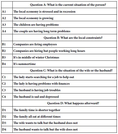
Following the choice of topic, create four questions which ‘tell a story.’ The questions are selected to move the ’story along’, but never appear in the test material (viz., the vignette described below). The hardest part of the Mind Genomics exercise often is the selection of the ‘appropriate’ questions because the questions will constitute the backbone of the vignettes, even though the questions never appear. As we see below, the four questions sketch out a reasonable, logical outline. Question B might have preceded Question A, but this decision was to follow the order below.

Question A: What is the current situation of the person?

Question B: What are the local constraints?

Question C: What is the situation of the wife or the husband?

Question D: What happens afterward?

The final part of the first step creates four answers to each question. The answers should be descriptive phrases which ‘tell a story,’ rather than simple yes/no terms which would not be found in a story. The objective is to create small stories, albeit stories without the necessary connectives. The stories or vignettes will comprise 2-4 phrases, presented in centered, stacked format, on a screen.

Table 1 shows the 16 answers, with the answer attached to one of the four questions. It is clear from Table 1 that each of the 16 elements is a simple description, with no hint of the emotional response of the members of the family to each other, although the element can describe the emotional condition of an individual with respect to the circumstances at large, such as elements C3 and C4 about the husband’s emotions in general. It is also clear that the elements paint short ‘word pictures’ and move beyond simply noticeably short and non-evocative phrases. The one element which is noticeably short is B4 (It’s summertime), which is meant to elicit the feelings about summertime.

At this point, it is important to note that the study appears to be simply notions, ideas thought up as convenience stimuli. That is true. The underlying objective of Mind Genomics is to make research easy, quick, iterative, and affordable. Unlike a great number of other research approaches, Mind Genomics encourages guessing about the correct test stimuli to use. Being able to iterate quickly, to pivot in an hour or two, means that the 16 answers or elements shown in Table 1, and indeed even the questions, can be tested in a study, the promising ideas kept and refined, the less than promising ideas discarded, and in their place new ideas introduced.

Table 1: The 16 elements (answers to the four questions)

table 1

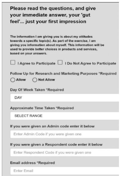
2. Field execution. The field execution comprises a short, 3-4 minute ‘interview’ with a respondent. The respondent remains totally anonymous, both in terms of disclosure of identity by the panel provider (Luc.id), and by the researcher setting up the experiment. For both Luc.id and the Mind Genomics technology, BimiLeap®, the requirement is for everything to be anonymized, unless specifically requested by the researcher, and accepted by the respondent.

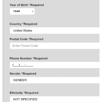
The online panel company, Luc.id, Inc., invites the respondents to participate. The respondents are compensated, but the details of the compensation are not relevant to the researcher. The respondents click on a link embedded in the invitation and are led first to a classification page, which thanks the respondents for participating, and which asks them to record their age, gender, and their marital status (question #3). This third classification question is in the purview of the researcher to write. For this study, the classification question was phrases as: What is your marital situation 1=single2=married3=living together4=divorced5=Not applicable

After the respondent completed the classification question, the respondent next read the orientation page, and rated 24 systematically varied vignettes, using the same rating scale. The BimiLeap program recorded the rating, the response time (time between appearance of the vignette on the screen and the rating), and then recorded the data in a database for almost-immediate analysis.

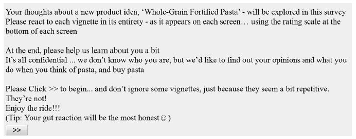
The respondents are introduced to the study by an orientation and a rating question. By design, the orientation is short. In this way, it is left to the specific elements to specify the situation. It will be the elements which will become the key to understanding the mind of the respondent. The less information in the orientation the more that the respondent will use the elements to drive the rating.

Here is a set of snapshots of families. Please read the full snapshot and tell us what will happen within the foreseeable future. Read the whole snapshot. Is it going to be peaceful, or do you sense some family violence brewing?

What will happen in the foreseeable future with this family?

1=peace and love …9=some violence(Bot=Peace, Top =Violence)

fig 1

Figure 1: The appearance of a test vignette on the smartphone

Figure 1 shows an example of the vignette as it would appear on a smart phone. The format is set up to make it easy to scan the vignette, pick out the relevant material (an almost automatic behavior), and then rate the combination.

To the unaided eye, the vignettes appear to be haphazard combinations of elements, thrown together at random. The presentation of these types of combinations ‘frustrates’ the respondent who is trying to answer ‘correctly,’ viz., to ‘get it right.’The impression of a haphazard combination is very far from the reality, however, it is important to keep in mind that the 24 vignettes are created according to a strict plan which ensures that each element appears equally, that all elements are statistically independent of each other, and that the data for each respondent suffices to allow for a regression model to be created for that one respondent. The latter feature ensures the ability to estimate the necessary parameters (coefficients), allowing for clustering or segmentation according to the pattern of coefficients.

Each respondent evaluated a specific, and unique set of 24 vignettes, some vignettes comprising two elements (answers from two different questions), some comprising three elements (answers from three different questions), and the remaining comprising four elements (answers from all four questions). Each element appears five times across the 24 vignettes designed for an individual respondent. By unique is meant that the vignettes tested by one respondent were mathematically identical to the vignettes test by other respondents, but the actual combinations were different for each respondent. This approach allows the Mind Genomics effort to cover a great deal of the so-called ‘design space,’ the combinations that could be created. The approach, called the permuted design method[15], makes the Mind Genomics approach a good tool to learn, even when absolutely nothing is known about the topic. One need not know the most ‘promising region’ to test, something which frees the researcher from losing out when the initial guess is incorrect. Each experiment covers a lot of the design space, with as few as 20-30 respondents.

One final point is important to reiterate. This point is the strategy of experimentation which sacrifices precision of measurement (averaging out the variability), replacing it precision by identify the pattern, even though the individual points are variable. The analogy in medicine is the the MRI, magnetic resonance imaging. The pattern emerges from the many different combinations tested. With 50 respondents, for example, the study here covers 1200 combinations. The underlying strategy is to permute these combinations, keeping the mathematical structure the same, but changing the specific combinations [15]. With the 1200 combinations tested in this study (minus a few possible duplicates across respondents), and with measurement at each point, each combination, we have the opportunity to evaluate many different regions of the ‘design space,’ see what works, and then redo the study, focusing on that part of the space. We have the benefit of evaluating many different combinations, and not having to know anything at the start. A few iterations, and a researcher can ‘home in’ to promising areas, viz., topics driving violence.

A total of 50 respondents participated, all from the United States. New subgroups defined as the three mind-sets, will be discussed below. For now it is simply relevant to think of these mind-sets as individuals with different patterns of response to the vignettes.

3. Relating elements to responses. The Mind Genomics point of view is that the valuable information is in the parameters of the model relating the presence/absence of the 16 elements to the ratings. The first step to create the model defines two new dependent variables, both from the rating. Recall that the rating scale is anchored on both side, with 1 being a response of ‘love’ and a 9 being a response of ‘some violence.’ We are interested in the ability of the elements to drive love or violence, respectively. In order to address the issue of two opposite objectives, we create two new binary variables, Love and Violence, respectively. These two newly created binary variables make the interpretation much easier when we look at the tabulated results.

The actual transformation is:

                  Rating of 1-3 transformed to 100 (Love), ratings of 4-9 transformed to 0 (Not love)

                  Ratings 7-9 transformed to 100 (Violence), ratings of 1-6 transformed to 0 (Not violence)

To complete the transformation, a small random number (<10-4) is added to all of the transformed ratings, in order to add artificial but miniscule variation in the newly created binary variables, Love, Violence. The addition of this small random number ensures that the dependent variable will have some minimal level of variability, required for the OLS (ordinary least-squares regression)o work, and not to crash.

In the presentation of the results, we will presently only the positive coefficients, AND NOT REPORT coefficients which are either 0 or negative, respectively. The underlying themes emerge more clearly when we focus only on the positive coefficients. The negative coefficient simply means ‘absence of’.

4. Relating elements to responses – extending the analysis to individual level models to create new to the world mind-sets. One of the hallmark benefits of the Mind Genomics approach is its ability to uncover mind-sets, defined operationally as different patterns of coefficients for the same set of elements and the same rating attribute. We will create one group of mind-sets, defined a separate, non-overlapping groups of responses who show similar patterns of coefficients, both for Violence and for Love, respectively. That is, we have two types of behaviors, violence (ratings of 7-9) and love (ratings of 1-3). We will create a separate pair of models for each of the 50 respondents, one model or equation for violence vs the 16 elements, and the second for love vs the 16 elements. The independent variables for each respondent were set up by the aforementioned ‘permuted design’, producing a valid experimental design for each respondent. As a consequence, OLS regression allows us to create a valid pairs of equations or models for each respondent.

To create the individual-level equation, we fit a simple linear equation, without an additive constant, doing so for each respondent, once for the 16 elements vs the response ‘violence,’ and for the same 16 elements vs the response ‘love,’ respectively. The calculation generates 32 coefficients, 16 coefficients for the equation for violence, and a parallel 16 coefficients for the equation for love. There are no additive constants in either model.

The clustering which follows is a purely mathematical effort. There is no effort to interpret the data at the tie of clustering, although such an effort might be viable For Mind Genomics studies the clustering produces easy-to-label clusters called mind-sets, easy perhaps because the test stimuli on which the clustering is based, coefficients of elements, use cognitively rich stimuli.

5. Patterns emerging from models. Once the respondents have been identified according to the relevant criteria (total, age, gender, relationship status, membership in the mind-set from clustering) the relevant data for a group are analyzed twice, once creating an equation for Violence (ratings 7-9 converted to 100, otherwise converted to 0), and once creating an equation for Love (ratings 1-3 converted to 100, otherwise converted to 0). This time the equation does have an additive constant.

Binary Variable (Violence or Love) = k0 + k1(A1)+k2(A2)…k16(D4)

The additive constant is the expected proportion of the responses to be 100 (viz., rating 7-9) when there are no elements. The experimental design introduced above ensures that all vignettes comprised 2-4 elements, meaning that the additive constant is a purely estimated parameter.

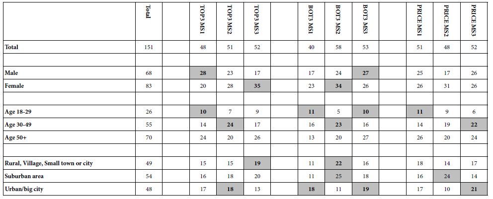
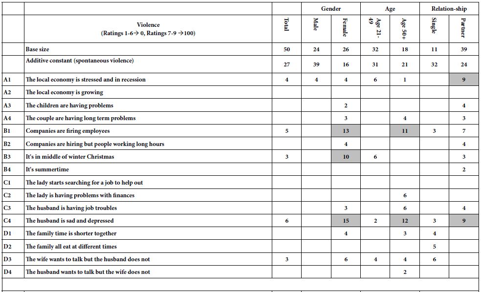
Patterns for ‘violence’: The additive constant can be interpreted as the expected percent of the responses the respondent will rate a vignette 7-9 in the absence of elements. Of course, that is not possible since by design all vignettes comprised 2-4 elements. Nonetheless, the additive constant is a valid measure, one that plays the role of a baseline feeling. The top of Table 2 shows the summary table for the response ‘violence’.

  1. The total panel is 27 – violence will be the outcome for one out of every four responses
  2. Males judge the outcome as violence far more frequently than do females(39 vs 16)
  3. Young people judge the outcome as violence more than do older people (31 vs 21)
  4. Single people judge the outcome as violence more than people with partners (married, in a relationship)

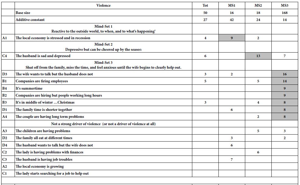
We now proceed to the individual elements, and the patterns emerging from the groups. As noted above, in the interest of clarity we do not present coefficients which are 0 or negative, but rather present only coefficients equal to or higher than 2. We also shade coefficients of +8 or higher, because it is around +8 that a coefficient reaches statistical significance (T value around 1.5 or higher).

Table 2 (Top; Violence) suggests no clear pattern by key subgroup, but some elements which drive expected violence, at least among some respondent groups. These trigger elements leading to expected violence are:

B1 – Companies are firing employees, as perceived by females and respondents aged 50+. This means that when these respondents read a vignette, the element B1 is likely to trigger the expectation of some violence occurring.

C4 – The husband is sad and depressed, as perceived by females, older, and those with current with partners.

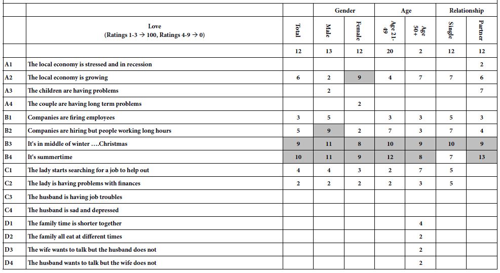
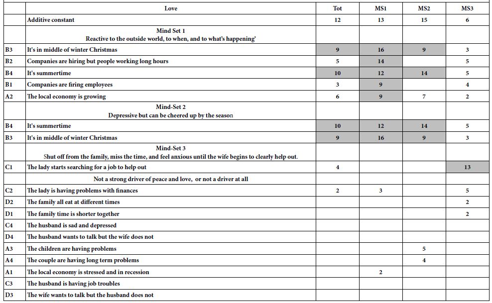
Patterns emerging for ‘love’: Table 2 (Bottom; Love) reveals very low additive constants, most around 12 or lower, except for the younger respondent (age21-49) showing a still-low additive constant of 20.

The two elements bringing almost universal love are descriptions of the season: (B3 – Middle of the winter Christmas) and B4 (It’s summertime)

We conclude from this first analysis that there are few strong differences among the groups. Only a few elements emerge to drive either violence or love.

Table 2: Models relating the presence/absence of the 16 elements to either violence or to love. The data come from the groups as they specified themselves in the up-front classification step.

table 2(1)

table 2(2)

6. How one element influences another (scenario analysis). The permuted experimental design brings with it an unexpected capability to uncover interactions among elements. The underlying experimental design is set up to make all the 16 elements statistically independent of each other. If every respondent simply evaluated the predesignated 16 combinations, it would be impossible to discover synergies between elements, where the presence of a pair of elements in the same vignette ‘turbocharges’ the rating, so the rating is much higher than one would predict from the simple sum of the coefficients.

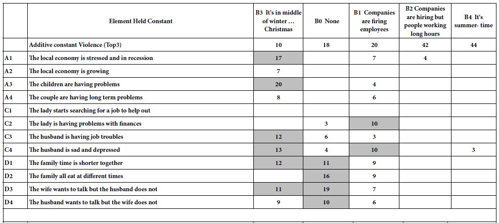
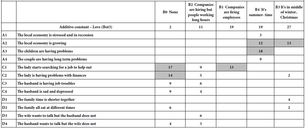
The strategy for creating the scenarios follows a set of simple, based upon the notion that each of the elements in the study appears five times for every respondent, and is absent 19 for every respondent. Let us now select one of the four questions, for example question B. Question B comprises four elements presenting information about the time of year, and what companies are doing, respectively. We consider our four elements to be strata, and sort all of the vignettes into the four strata defined by the elements, as well as into the fifth stratum defined by all the vignettes which, by design, lack an element.

The previous exercise creates five strata. In each stratum, the element B is held constant, or does not appear. We now have five new data sets, each with elements from Questions A, C and D present. We simply run two sets of five equations, using as the dependent variables Top3 (Violence) and Bot3 (Love), respectively. The 12 independent variables are A1-A4, C1-C4, and D1-D4.

Table 3 show the five regression models. Each column corresponds to one of the five strata, defined by B1-B4, as well as B0 (B absent from the vignette). Each row corresponds to one of the 12 remaining elements. The top of Table 3 shows the coefficients for Top3 (violence), sorted by ascending order of additive constant. The bottom of Table 3 shows the coefficient of Bot3 (Love), sorted once again by ascending order of the additive constant.

Table 3 shows us much great performance of the elements as drivers of violence and love, respectively. Once the elements are constrained to be fixed in a vignette, they set the ‘stage’ for the ideas. We can see various new patterns emerge, allowing a deeper insight into the topic. For example, when we look at the model for B3 (it’s in the middle of winter Christmas), we see a low proclivity for violence (additive constant is 10, the lowest basic proclivity). ON the other hand, there are specific events which occur which substantially increase the likelihood of violence. Examples are A1 (The local economy is stressed and in recession), and A3 (the children are having problems).

Let us compare the violence expected in winter to the violence expected in summer. We now turn to the last column, for element B4 held constant. The additive constant is much large, an extraordinary 44.Yet, there are no other elements which drive expected violence.

We now move to the bottom of Table 3.We see that the same element, B3 (it’s in the middle of winter. Christmas) brings happiness, viz., synergizes with A2 (the local economy is growing).And, when it is summertime, rather than wintertime, element A3 (the children are having problems) bring love to the family, not violence. That is, the same element (A3)can drive violence (winter) or drive love (summer).

It is patterns like these which are the ‘value add’ to a Mind Genomics cartography. We are able to get a sense of new patterns, some of which make intuitive sense, and some which may spur an ‘aha’ moment.

Table 3: Scenario analyses, holding constant each of the four elements (and the no-element) from Question B, and estimating the model using the remaining 12 elements.

table 3(1)

table 3(2)

7. The allure of mind=sets as organizing principles. Our previous analyses of the data suggested some effects, such as love expected to emerge during two special times, Christmas in the winter and during summer, respectively. One can investigate the literature of the social and psychological sciences, and in doing so discover these disconnected nuggets which intuitively feel as if they are ‘weak signals’ emerging from a deeper, more coherent reality. The problem is that these signals emerge unexpectedly, and do not allow for a deeper investigation without first requiring a hypothesis of just ‘what is happening’.

Mind Genomics circumvents these problems, first by providing a method of clustering based upon a small, tightly defined topic, and then allowing the research to be done efficiently, inexpensively, and in a manner which moves stepwise through the problem in simple and illustrative steps. The clustering method is totally a theoretical, in terms of the meanings of the clusters. The clusters are labelled by which elements score highest and tell a ‘coherent’ story. The method of clustering is known as k-means clustering. The ‘distance’ between people in k-means clustering is known as ‘D’ defined as (1-Pearson R), where the Pearson R is the Pearson linear correlation between each pair of respondents, computed on the 32 coefficients [16].

The clustering performed on the data did not make any assumptions, because none needed to be made. The models were created for each respondent. The two decisions were to combine the models for one individual (violence and love together to extract people similar in both), and then to extract three mind-sets. Two, three, four, and even more mind-sets could have been extracted. The ideal is to work with as few mind-sets as possible (parsimony), but have each mind-set tell its own coherent story (interpretability). The data suggested that two mind-sets may have been the more parsimonious, but the patterns of the coefficients were not clear. Too much information seemed to cross the mind-sets, suggesting the need for a third mind-sets.

The results from the clustering to generate three mind-sets appear in Table 4 Again, we show only the additive constant, and the elements with positive coefficients for each mind-set. From these, we might name the mind-set. The Top of Table 3 shows the results for the response ‘violence’, the bottom of Table 3 shows the results for the response ‘love’. We will present the additive constant, and then piece together a story from the strong performing elements for that mind-sets.

Mind-Set 1 = High violence constant (42), very low love constant (12). Mind-Set 1 is prone to violence when the economy is stressed and in recession, but that is all. Mind-Set 1 is prone to love when things are better, when its summer and winter and when things are going well. Mind-Set 1 is also, however, just as prone to love when people are getting fired. Mind-Set 1 might be called reactive to the outside world, to when, and to what’s happening’

Mind-Set 2 = lower violence constant (24) and very low love constant (15). Mind-Set 2 is probably a person who is depressive but can be cheered up by the season.’

Mind-Set 3 = lowest violence constant (14), lowest love constant (6), strong reactor to the family situation. Mind-Set 3 is most likely to shut off from the family, miss the time, and feel anxious until the wife begins to clearly help out.

The important thing about Table 3 is that the elements which are strongest appear to paint a picture, which makes intuitive sense. Not everything ‘hangs together’ but we are dealing with a small sample of individuals, and the first effort, done in the period two days. The elements can be refined to expand the focus.

Table 4: Models relating the presence/absence of the 16 elements to either violence or to love. The data come from the three mind-sets which emerged from clustering. Only the positive coefficients are shown.

table 4(1)

table 4(2)

Discussion and conclusion

As we see from the cursory data from 50 respondents, the data provided by Mind Genomics is rich, indeed far richer than one might expect from a method emerging out of consumer research. One of the reasons for the rich information comes from the effort of Mind Genomics to provide a context for each stimulus. Rather than responding to a set of disconnected questions, the respondent evaluates a unique set of 24 vignettes, each of the vignettes more likely to tell a story than a single question would be.

In our study we take many pictures of the family and ask what might be happening for that particular picture or vignette. It is only later that we put together the individual snapshots (responses to the vignettes) into a coherent whole, an action made straightforward by the use of individual-level experimental designs, and permuted experimental designs. Mind Genomics capitalizes on both, identifying pictures from disparate combinations, and covering a lot of the ‘design space’ of possibilities, using the strategy of permuted experimental design.

The study reported here can be considered to be a cartography, an exploration of the ‘territory’ of the topic, rather than an attempt to confirm or falsify hypotheses. Mind Genomics gives us an opportunity to move in a variety directions, in the spirit of exploratory research, mapping the mind of people as they think about stressful situations, or even as they live through the stressful situation. The objective is not to accept or reject a hypothesis about ‘how behavior works’ or ‘how the mind works.’ Rather, the objective is to find repeating patterns of behavior, or stated patterns of thinking, either separate from the situation, or even in the middle of the situation. A good example of the approach can be found in [17], which deals with the types of behavior that teens want from doctors. That type of information is gathered in the same spirit as these data, namely understanding behavior in stressful situations.

The data lend themselves to the systemized creation of knowledge, literally at an industrial scale, across topics, countries, people, and external situations. For example, we might run this same experiment during several seasons of the year, and in several venues with varying economic conditions, as well as with people who are known to be prone to family violence versus people without that history. All of these approaches will end up creating, in rapid pace, an affordable database of the mind of family violence and family affection, a database that can be extended world-wide with very little effort. The patterns and the increased knowledge, and perhaps even many more ‘ah ha’ moments await the research. The approaches were laid down more than two decades ago, but the methodological advance is fresh, and the data continuing to pile up, in well-managed databases which maintain their value year after year because they reveal the nature of the ‘mind’ and ‘mind-sets’ confronted with situations inevitable emerging from the daily life of people world-wide[18-20].

References

  1. Ammerman RT, Hersen M (eds) 2000 Case studies in family violence. Springer Science & Business Media.
  2. Denzin NK (1984) Toward a phenomenology of domestic, family violence. American Journal of Sociology. 90 : 483-513.
  3. Momirov J, Duffy A (2011) Family violence: A Canadian introduction. James Lorimer & Company.
  4. Anderberg D, Rainer H, Wadsworth J, Wilson T (2016) Unemployment and domestic violence: Theory and evidence. The Economic Journal126 : 1947-1979.
  5. Aizer A (2010) The gender wage gap and domestic violence. American Economic Review100 : 1847-1859.
  6. Showalter K (2016) Women’s employment and domestic violence: A review of the literature. Aggression and Violent behavior31 : 37-47.
  7. Rotton, J., & Cohn, E. G. 2002. Climate, weather, and crime. In : RB Bechtel, A Churchman (Eds.), Handbook of Environmental Psychology. John Wiley & Sons, Inc. pg : 481-498.
  8. Shortlands ND. https://www.shortlands.co.uk/crisis-at-christmas/
  9. Card D, Dahl GB (2011) Family violence and football: The effect of unexpected emotional cues on violent behavior. The Quarterly Journal of Economics126 : 103-143.
  10. Moskowitz HR, Gofman A (2007) Selling Blue Elephants: How to Make Great Products that People Want Before They Even Know They Want Them. Pearson Education.
  11. Moskowitz, Howard, James Wren, Petraq Papajorgji (2020) Mind Genomics and the Law. 1st Edition. LAP LAMBERT Academic Publishing.
  12. Moskowitz H, Prendi V, Gere A, Harizi A, Papajorgji P (2021) Mind-sets of worried citizens and the ‘real-world experiment’ of Covid-19: A mind genomics cartography. Edelweiss Applied Science and Technology 41-49.
  13. Gere A, Papajorgji P, Moskowitz HR, Milutinovic V (2019) Using a Rule Developing Experimentation Approach to Study Social Problems: The Case of Corruption in Education. International Journal of Political Activism and Engagement6 : 23-48.
  14. Mariampolski H (2006) Ethnography for Marketers: A guide to Consumer Immersion. Sage.
  15. Gofman A, Moskowitz H (2010) Isomorphic permuted experimental designs and their application in conjoint analysis. Journal of sensory studies25 :127-145.
  16. Likas A, Vlassis N, Verbeek JJ (2003) The global k-means clustering algorithm. Pattern Recognition, 36 : 451-461.
  17. Gabay G, Moskowitz HR (2015) Mind Genomics: What Professional Conduct Enhances the Emotional Wellbeing of Teens at the Hospital?. Journal of Psychological Abnormalities.
  18. Moskowitz HR (2012) ‘Mind Genomics’: The experimental, inductive science of the ordinary, and its application to aspects of food and feeding. Physiology & behavior107 : 606-613.
  19. Moskowitz HR, Gofman A, Beckley, J. & Ashman, H., (2006) Founding a new science: Mind genomics. Journal of sensory studies21 : 266-307.
  20. Boserup B, McKenney M, Elkbuli A (2020) Alarming trends in US domestic violence during the COVID-19 pandemic. The American Journal of Emergency Medicine38 : 2753-2755.

Status of Menstrual Dignity during the COVID-19 Pandemics

DOI: 10.31038/AWHC.2021444

Abstract

Background: Violence against women takes different forms, often reflecting cultural patterns. Forced segregation and other dangerous or at least discriminatory practices during menstruation can be observed in a number of cultures, such as Nepal, but also in other regions. The present pandemic with its special risks and lockdown measures must be expected to potentially cause additional problems for women in the critical time of menstruation.

Aims and methodology: The aim of our study was to collect information on the experience of women in different regions and identify risk factors for such practices, such as education, health belief systems and bias in the communities together with the impact of the COVID pandemic on these factors. The survey was conducted online to keep safety protocols necessary during the SARS 2 pandemic. To identify possible key factors we conducted a qualitative/mixed method survey resulting in categories and vivid descriptions relating to violence and discrimination. 139 participants, (age range 13-48 years, 85.8 percent female, else LGBT) from different countries, including both low-economy countries with high rates of reported discrimination such as Nepal and India, but also from the US participated in the survey.

Results: Patients reported experience of bias and insufficient or incorrect information by parents, and later in the communities. Lockdown measures impacted in some cases, but in general to a lesser degree on access to dignified hygienic measures required during menstruation, as compared to before the pandemics, but was reported to increase the social stress and reduce social support. Shame, insecurity and distress during menstruation continued and were described as main adverse factors influencing well-being and psychological health.

Keywords

Women, Gender, Menstruation, Discrimination, Dignity, Pandemics, COVID-19

Background

The World Health Organization (WHO) confirmed the coronavirus outbreak as a pandemic on 11 March 2020. From the outset of the pandemic, the United  Nations and various countries  are working towards a large-scale, coordinated, and comprehensive health response. Women are disproportionately affected by the COVID-19 crisis because of the gender and social norms combined with the disruption of services and the special challenges of factors such as menstruation or pregnancy [1]. The impact must be seen     as multifactorial, including the impact of infection, long COVID, vaccination, and the different COVID prevention and lock-down measures. They have been documented to affect some population groups such as women and migrants in different ways [1-3].

A number of publications have  also  reported  the  impact  on the physical health of women such as sex hormones, fertility and spontaneous abortion [4-6] and on mental health [7]. Several authors, such as Abuhammad et al. have further observed increased problems related to domestic violence in the Pandemics [8,9]. Abdelbadee et al. have further drawn attention to the specific problems to be observed in low-income countries [10].

The pandemic has been exacerbating existing inequalities between women and men in almost all areas of life [3]. However, menstrual discrimination (taboos, stigma, abuses, restrictions, discriminations) has not been studied in the context of the pandemic at least in Asia  in spite of the well published earlier concerns in regard to the politics of menstruation during the pandemic by Jahan [11], by the first data published by Aolymat on women in Jordan [12] and several other authors [13-15].

Therefore, this study was conducted to fill this gap mainly by contributing to a better understanding of menstrual dignity and the experiences of women and LGBTQI during menstruation and observed changes during the COVID-19 pandemic.

Methodology

The study adopted a mixed-method qualitative method integrating qualitative components based on open questions with a short structured questionnaire to elicit general social data and basic information on menstruation related health literacy developed for  the study. We also decided to use a multi/transcultural approach by recruiting participants from different countries and cultures as culture has been identified as a major factor in menstrual practices and related health belief systems [16]. The survey modules separated questions regarding the situation in general and before the pandemic and those regarding the changes observed during or due to the pandemics.

A survey of 139 participants from different countries was conducted using an open online platform developed for the project.

Not all respondents filled out all items in the survey, though all participants answered to at least 90% of the questions. The respondents had been recruited through a public platform delivering the survey. All participants gave informed consent during registration, data were stored anonymised on a safe server and will be erased in due time following common data safety protocols.

The age range of participants was between 13-48 years, 85.8 percent were female and 11.2 percent and the rest identified themselves as LGBTQI (Lesbian, Gay, BiSexual, TranSex, Queer and Intersex). The participants were from ten countries: Bangladesh, Bhutan, India, Israel, Madagascar, Namibia, Nepal, Philippines, Uganda, and USA. All respondents had education backgrounds ranging from higher education to master’s degree; 22.1 percent finished high school;

58.8 percent held bachelor degrees and 19.1 percent master’s degree as highest level of education. Only nine percent of the respondents revealed that they were people with physical or mental disabilities at the time of responding to the online survey.

Findings

General Findings

Knowledge about Menstruation

The respondents reported to have learned about menstruation from different sources, which included mainly their mothers, other family members, school, internet, or from friends. This happened in some participants when they were between age 5-13 years, and in the majority only when they were 10-12 years old.

In the qualitative part of the survey, using the open questions based on an interview guideline, respondents reported:

‘My grandmother gave me a “menstruation talk” starting at age eight up till age 13 and gave me information that was appropriate at each age as I come from a family that has a high risk of menstrual problems. Post age 13, I have received informed from friends & gynecologists’.

‘Although school syllabuses contain reproductive and sexual education, students are not properly provided with knowledge. I learnt most of it from my mother and later by studying myself ’.

‘When my mother was menstruating, my father asked for help from me while cooking.’

Initial Reaction

Respondents stated that their first reactions after having the menstruation were as follows.  Sixty-six  percent  of  respondents  felt scared, seven percent felt sick, and seven percent considered menstruation normal and reacted accordingly. Ten percent of responses on this question noted that the question did not apply to them (all members of the LGBTQI group), and another 10 percent had an ambivalent experience.

‘When I looked into my pants, I was devastated, thinking I was about to die. Nobody likes looking at blood, in whatever sense’.

‘Did I eat something wrong, or did I had an accident that makes my internal parts bleed’

‘Damn, will I survive with this massive loss of blood?

‘During menarche, I thought I was exposed to some deadly disease and angrily went to my mother and claimed that I feel I would die soon as I am bleeding. Then, my mother explained that you are menstruating and it’s a natural process which a woman has to undergo every month’.

Discrimination during Menstruation

Even in regular menstruation, many of the 77 respondents on this items experienced discrimination during menstruation directly and indirectly, as described in the open responses. Mostly, respondents described discrimination as verbal, emotional, as denial of menstrual products, and as impaired mobility. Out of 77 respondents, 23 participants stated that they remained silent while experiencing discrimination. They felt hurt, traumatized and pained though they did not do anything inadequate in their own perception. This group simply tried to ignore discrimination and most of them stated they had no energy to “fight back”. Some of them also said that they felt like “avoiding people”, “running away” or it her acts of social withdrawal.

‘I would not want to be a part of the community where people do not understand and respect a natural phenomenon as such’.

‘I have left an office internship because my supervisor wasn’t sensitive enough. So instead of working from the office, I chose to work in a different department in the same organization. I have also complained about this insensitive behaviour of the supervisor’.

‘I feel inferior to the persons who perpetuate violence towards me, and I feel pressured by societal expectations to abide by the greater publics expectations, so therefore I do not feel empowered to speak up even though I am aware I should do so.’

Out of 77, 49 respondents tried fighting back. They educated  and empowered themselves by sharing facts and then started raising questions about the experienced acts of discrimination. Some reported to have argued with community and family members, and to have used different forms of direct confrontation, including screaming. Further they reported engaging in teaching about natural phenomena and human rights in the community, and involving community members in a dialogue on menstruation.

‘I tried understanding why this is happening and why was it considered a taboo. I usually have these conversations with my mother because she is usually the one who perpetuated the discrimination and had herself not experienced any problems with my family. Still, while visiting the village, I hide the fact that I’m menstruating.’

‘When it comes to PMS comments and menstrual stigma from peers, I educate them politely. However, for elders, I have given up on explaining because they won’t budge’.

However, even while fighting back, they experienced feeling tortured, weak, sad, annoyed, oppressed, helpless, depressed, embarrassed, frustrated, worthless, tired, ashamed, guilty, disappointed, and awful (using the verbs in the qualitative part of the online review). Only few positive emotions were reported, such as feeling proud, or courageous.

‘Once, while I was visiting Lonavala, there was a temple I wanted to see, and I couldn’t because I was during the period. So I asked my mom, “Why can’t I go inside the temple just coz I’m bleeding” she told me, “you shouldn’t question faith”!!! And I felt very bad. I wanted to see the temple from the inside. But, I was so damn eager to see it, and I couldn’t’.

‘Very bad. Life on this planet exists due to the occurrence of menstruation, and they say we are weak for having it. Really!’

‘I feel disappointed at our education system and anger towards those conditioned to perpetuate discrimination by patriarchal mind sets’

‘I would surely feel shame, that’s awful, but it’s always the first emotion I feel when someone perpetuates some sort of violence on me. But then, I’ll call back and feel courageous. Then, last, I’ll be sad about how people can be so rude and uneducated’.

Openness Regarding Menstruation, Disclosure

Only 29 respondents stated that they freely talk with family members, in most cases because they are health workers (menstruator or non-menstruators) and asked for medicine or pads without any hesitation.The rest of the respondents (n-59) talked only with female members of the family such as mother, elder sister, grandmothers, and aunts and their discussions were more focused on ‘do’s and ‘do not’ including restrictions associated with menstruation, menstrual products, and menstrual symptoms or illness.

‘Yes, I talk about menstruation with my family. Talks would be something about how to maintain good hygiene during periods and techniques to ease cramps’.

‘With my mother only. Not my sister or father. It is very awkward. I only ever ask her for tampons when I run out. I spoke to her when  I was younger about what age she got her first period and how to use tampons and pads.’

‘As my father does not menstruate, and we were taught not to speak of “these things” with anyone other than mother, my conversation is mostly limited with her’.

80 respondents remained silent in public about menstruation, thinking for example that “it was disrespectful towards elder members of the family”. They stated they did not receive support from the family and considered it a matter of “hush and girl thing” (personal or private). Reasons mentioned included “Men should not know anything”, “conservative family”, “they hate the topic”, “would be avoided by men”.

“Maybe in African cultures, it is regarded as a taboo. However, we are fighting for fundamental rights, and everyone could be a part of this”.

“Because my parents believe menstruation should be kept a secret and that it is not conversation meant for the living room”.

However, respondents knew that their friends had been menstruating through observation of  their  various  behaviors,  which included blood stained clothes, their experiences of severe cramps, their being more emotional than usual, being hesitant to walk or to walk with precaution, the increased frequency of toilet breaks, avoidance of regular activities, from whispering among girls friends, asking for a favour like a pad, and by their having “pimples”. Segregation was common in their experience.

‘In Islam, a person is unable to perform “ablution” because it needs proper hygiene, so the person cannot perform religious duties’

‘In our culture, girls stay away and are considered untouchable. They are restricted from staying anywhere and from touching anything casually. They shouldn’t touch anybody. In the case of males, they shouldn’t even go nearby.’

‘Yaa. In our society, they stay separately during periods and wear old clothes. So it can be known easily.’

Anxiety during Menstruation in the Bathroom

Only 23 responses registered that they worried about using the toilets at home due to fear  of staining the blood, lack of water, fear of getting scolded, and running out of the menstrual hygienic aids. Respondents reported that they “avoided anybody who knows about the state of menstruating”, its being “like a murder scene”. Some reported also fears including “fear of contamination from the toilet”, “the sound of the opening of the pad”, and “fear of some household members”.

‘As you can touch nothing, you should beg for being handed everything. If you use your bathroom, it should be cleansed.’

‘Fear of getting scolded if the floor gets blood on it, lack of water supply-inability to flush the blood out, fear of getting scolded for forgetting used menstrual products wrapped in the bathroom after taking a shower.’

Understanding of Dignified Menstruation

A total of 62 percent of respondents mentioned that they would perceive freedom during menstruation as dignified menstruation. They considered that hygienic products (access to menstrual pads at home and workplace), freedom of individual behaviour, and family support as being the elements to make menstruation dignified.

Menstruation during the Pandemic

Out of 104 responses, fifty participants expressed that they experienced increased direct and indirect discrimination as compared to before the pandemic. They expressed varieties of violence in this context: physical (once), verbal, emotional, and denial of services. They reported not being allowed to go to the temple, not allowed to cook food, not allowed to consort with their husbands, prohibition to touch some plants (Tulasi), etc.

In the part of the questionnaire asking for experiences first observed during the pandemics, they reported:

‘”seems like you’re ALWAYS on your period,” “stop using it as an excuse,” “don’t you dare bleed on my bed,” not much.’

“One of my friends was beaten because she touched a water purifier.”

‘My brother couldn’t really understand when I first menstruated. People wouldn’t talk about this subject. He even complained about the smell of the blood. He would also force me to do my chores, and I really felt bad because he found it was unfair that I would go to sleep because of some “random illness once a month.”

Respondents experienced difficulties due to travel restrictions to purchase medicine for pain management and menstrual products, as online orders popular in high-income countries during the pandemics are not always available or affordable. On the other hand, when for example the government in India announced a COVID relief package, the menstrual pads were not considered essential by the authorities.

Still, only few of the participants (n= 10) reported that they run out of menstrual products, experienced scarcities, or experienced increased expenses, especially after the second and third months     of the lockdown . Several participants reported that they were not aware that the frontline health (pathologists, nurse, doctors etc.) workers supporting menstruation practices struggled so  much during menstruation due to lack of extra PPE (Personal Protection Equipment’s), menstrual products, and hygiene facilities at their workplace, while others commented on the situation especially in India, as mentioned before. Even the media highlighted the scarcity of toilet paper but did not care about menstrual products to cover in their media, as did some governments in their support emergency plans described above.

‘When the Indian government was making a list of industries that need to operate during the lockdown to provide necessary items, menstrual products were not included in the initial stage…”

Such restrictions during menstruation were accented during COVID-19 [11], and the Pandemic can be seen as discrimination and inequality in health care as in the above example. Women cannot speak about the discomforts and problems openly, cannot move freely, have to work with discomfort and pain, have difficulties in getting a shower and wash their belongings, feel ashamed when buying pads, feel pressure all the time even when they are at home with family, and expressed that they felt isolated or were marginalised even before the pandemic.

‘Girls are treated like as male COVID-19 patients (without special consideration)’

‘I always have, pandemic or no, been flabbergasted by the rules of not entering temples during periods, a duality of our society where you are fascinated by the femininity of goddesses but are filled with stigma when it comes to menstruation.’

‘Women should not talk about it to anyone, especially boys, because it makes you lose dignity. To “control the flow of my blood” and not to make a mess on my bed’.

‘We have to work very hard though we are agonizing in pain while the men of the house just sit and relax with no cramps or anything’.

‘Not able to use the kitchen. I need to ask for someone else to provide something like hot water. The situation is the same during the pandemic as before’.

‘This time, I had gone to my husband’s home in lockdown. I was asked not to enter the kitchen for four days and avoided drinking milk tea too. I have to use all utensils separately. I feel so bad, but I follow it because I was tired of cooking every morning to evening for about four months. Otherwise, I wouldn’t tell anybody. But secretly, I entered the kitchen to get water and food.’

Many menstruating women with a disability, transmen, immigrants, and refugees had suffered more discrimination during menstruation. They were compelled to use old clothes due to the lack of availability of menstrual products. However, only few reported feeling ashamed in managing menstrual products in front of the men’s family members, including children.

‘During the COVID buying PAD was the main issue trans-man. However, they can’t buy the PAD at the time of menstruation because shop owners ask many more questions and they can’t answer, so they use a single PAD for up to three days too’.

Only few of the members of this group thought that the menstruating persons were affected more by the pandemic due to their bleeding status.

Earlier Existing Practices of Segregation can be Accentuated

‘My uncles and aunts in the village think that menstruating women are more likely to develop COVID 19, so they isolate them for 14 days when menstruating. However, it’s not a very logical conclusion.’

In addition to these practices, some respondents also reported increased difficulties like menorrhagia, uneasiness, or the need to work more due to the absence of domestic help during the pandemic. Similarly, participants reported that they could not buy pain killers to ease the cramps, and their period to be irregular due to lack of exercise or change in lifestyle in this situation. Likewise, some participants used the pad sparingly to minimize the waste and to better hide from non-menstruating sisters and other family members,

‘Have to work more at home as domestic helpers are not available because of COVID-19 so I have no rest and have to work through pain’.

‘Since I am not at school, during my  periods, I am just in bed   all day crying until the pain passes. Because I can’t go out to buy painkillers, as they are more expensive than ever, and I consequently am in dire need to distract myself from the pain and focus on studying or something. Sometimes, I exercised heavily to dull the pain’.

Other women reported “I used few products to avoid the waste in our bins. I am worried that my non-menstruating sister or father will see the products in the bin and be embarrassed.”

Use and Management of Menstrual Products during the COVID-19 Pandemic

Regarding use of menstrual products, from the 106 participants who responded to this part of the survey, 82 participants used menstrual pads. Three used menstrual cups, and one used tampons. Respondents considered themselves privileged more than others in many ways; such as “living in urban areas”, by an “online supply”, and because of “access to money”. Participants bought menstrual pads from the grocery shop, pharmacy, and online, as they were open even during the lockdown. Few of them purchased in bulk before the imposing of lockdown. Therefore, most respondents, but depending on the local situation, continued the use of menstrual products as before.

‘All pharmacies are open since the number of COVID-19 cases is not very high in my area.’

‘I always bought a big pack of sanitary pads that is sufficient for 3 4 months, sometimes more … so I didn’t feel any shortening.’

‘I’m fortunate enough to have easy access to products. Medicine shops are open. They are available there’.

‘I use a menstrual cup. It’s pretty hygienic and reusable, plus it’s so comfortable I almost forget that I’m on my period’.

‘I had to “stock-pile” tampons before the lockdown, as we are not going to the shops often enough. I am managing okay, but we would be in a difficult situation if we hadn’t had money to buy extra tampons.

A total of ten respondents applied alternatives to manage the menstrual blood during lockdown like sleeping, or cloth pads because of financial limitations as the work and salary of their parents were interrupted.

‘It’s been quite challenging mainly to the girls in my community, lack of money to buy sanitary pads since also parents are no longer working’.

The transmen suffered much when they had to get out and buy the pads.

‘It’s pretty tough because it’s not like I can run to shops when I’m out of pads’.

Regarding waste management of such menstrual products, 75 respondents said that they were practicing as usual by throwing them in a in garbage tank either at home or in the municipality, seven burned, five re-used the products (cups and cloth), and one buried them in their field. Thus, they did not have significant problems managing the waste due to COVID-19. However, they struggled to wrap them up in newspapers, plastics, by hiding them underneath of bed, etc. due to already pre-pandemic taboo and stigma around menstruation.

‘I wrap them in paper and throw them in the dustbin, which is collected by the municipality vehicle garbage.’

‘Hardest thing ever. I keep collecting used pads for 2-3 days under my bed. Then, later, when there’s no male member around, I cover myself and throw it in the bin downstairs.’

25 (total 76 responses) respondents reported hiding their menstrual pads and increased increased problems during the pandemic. They experienced irritation, sadness due to the unavailability of the dustbin, and a few experienced foul odors, unhygienic conditions and felt shy in front of others.

One respondent described her experience “I don’t like the smell of the product and my blood. And I don’t want my family to see and smell of that disposed stuff. I don’t want my family to see something that was near my private area. And I am also worried that the adhesives might give up, and the folded pad opens up, revealing a “bad” scene”.

Discussion

Pandemics or any other disaster can have a severe physical impact on menstruation and the health of women [17-20]. Menstruating women are experiencing increased discrimination during the COVID-19 pandemic due to silence  and  ignorance  about menstruation, but also in logistics and access to menstruation pads or cups during the pandemics as observed by our group. This can result in difficult situations for both the women and for their health care workers, as reflected in extreme measures – as example frontline health workers reportedly used birth control pills to stop menstruation at Wuhan, China. However, women have a dire need  for menstrual dignity through more freedom during menstruation. The impact of menstrual discrimination has a multi-level impact that affects mental, physical and social health and might lead to violation of the human rights of the women. The needs and priorities of women should be scrutinized and need to be addressed even in shifting priorities of service providers during quarantine, isolations, hospitals, travel restrictions and curfews, the ongoing financial crisis. Scarcity of menstrual products and other essentials in some countries might be affected to a different degree. Communities and families need education and improved health literacy to fight health belief models leading to discrimination or violent acts such as forced segregation.

The observations in our mixed method study are limited by the small sample size and by the methodology based on an online survey and can therefore not provide representative data on the countries of the participants, that can be generalized. Still, the results identify and highlight some of the problems pre-existing and those accentuated or created during the pandemic.

Conclusion and Recommendations

Menstrual discrimination prevails in many countries and the problem was neglected across all the countries during the COVID-19 pandemic in our study. Since menstrual discrimination is a form of gender-based violence, it is continuously manifested in various forms. Based on the findings, our recommendations are as following:

  1. Information should be available everywhere in numerous languages on the physiology of menstruation and all aspects of menstrual dignity to increase health literacy for all genders and decrease stigma and discrimination based on inadequate knowledge and traditional cultural practices or belief systems.
  2. The menstrual products should be included in the COVID-19 response packages, and other humanitarian response materials.
  3. The provision of water, menstruation-friendly toilet/bathroom, hand sanitizers, and a mechanism for safe, discrete and low barrier waste management needs to be ensured in all settings, including temporary shelters, as explored by some authors [21].
  4. Programs as described in 1, focusing on menstrual dignity need to be continued across all programs as a cross-cutting concern.

References

  1. Abate BB, Kassie AM, Kassaw MW, Aragie TG, Masresha SA (2020) Sex difference in coronavirus disease (COVID-19): a systematic review and meta-analysis. BMJ Open 10: e040129. [crossref]
  2. Türkan Akkaya-Kalayci ODK, Thomas Wenzel, Anthony Chen VC, Zeliha Özlü- Erkilic (2020) The impact of the COVID-19 pandemic on mental health and psychological well-being of young people living in Austria and Turkey: a multicenter study International Journal of Environmental Research and Public Health 17: 9111. [crossref]
  3. Abufaraj M, Eyadat Z, Al-Sabbagh MQ, Nimer A, Moonesar IA, et (2021) Gender- based disparities on health indices during COVID-19 crisis: a nationwide cross- sectional study in Jordan. Int J Equity Health 20: 91.
  4. Cosma S, Carosso AR, Cusato J, Borella F, Carosso M, et al. (2021) Coronavirus disease 2019 and first-trimester spontaneous abortion: a case-control study of 225 pregnant Am J Obstet Gynecol 224: 391 e1-e7. [crossref]
  5. Xiong Z, Li P, Lyu H, Luo J (2021) Observational Study of Working from Home during the COVID-19 Pandemic Using Social Media JMIR Med Inform.
  6. Bagli I, Ocal E, Yavuz M, Uzundere O, Bozkurt F (2021) Maternal deaths due to COVID-19 disease: The cases in a single center pandemic hospital in the south east of J Obstet Gynaecol Res.
  7. Ahorsu DK, Imani V, Lin CY, Timpka T, Brostrom A, et al. (2020) Associations Between Fear of COVID-19, Mental Health, and Preventive Behaviours Across Pregnant Women and Husbands: An Actor-Partner Interdependence Modelling. Int J Ment Health Addict 1-15. [crossref]
  8. Abuhammad S (2021) Violence against Jordanian Women during COVID-19 Outbreak. Int J Clin Pract 75: e13824. [crossref]
  9. Abujilban S, Mrayan L, Hamaideh S, Obeisat S, Damra J (2021) Intimate Partner Violence Against Pregnant Jordanian Women at the Time of COVID-19 Pandemic’s J Interpers Violence 886260520984259. [crossref]
  10. Abdelbadee AY, Abbas AM (2020) Impact of COVID-19 on reproductive health and maternity services in low resource countries. Eur J Contracept Reprod Health Care 25: 402-404. [crossref]
  11. Jahan N (2020) Bleeding during the pandemic: the politics of menstruation. Sex Reprod Health Matters 28: 1801001. [crossref]
  12. Aolymat I (2020) A Cross-Sectional Study of the Impact of COVID-19 on Domestic Violence, Menstruation, Genital Tract Health, and Contraception Use among Women in Am J Trop Med Hyg 104: 519-525. [crossref]
  13. Wilbur J, Kayastha S, Mahon T, Torondel B, Hameed S, et (2021) Qualitative study exploring the barriers to menstrual hygiene management faced by adolescents and young people with a disability, and their carers in the Kavrepalanchok district, Nepal. BMC Public Health 21: 476.
  14. Thapa S, Aro AR (2021) ‘Menstruation means impurity’: multilevel interventions are needed to break the menstrual taboo in BMC Womens Health 21: 84. [crossref]
  15. Levitt RB, Barnack-Tavlaris JL (2020) Addressing Menstruation in the Workplace: The Menstrual Leave In: Bobel C, Winkler IT, Fahs B, Hasson KA, Kissling EA, Roberts TA, editors. The Palgrave Handbook of Critical Menstruation Studies. Singapore 561-575. [crossref]
  16. Paudel Radha A, Mili, Kletecka-Pulker, Maria, Wenzel, Thomas (2019) The Construction of Power in Nepal: Menstrual Restriction and Rape Arch Women Health Care 2.
  17. Li F, Lu H, Zhang Q, Li X, Wang T, Liu Q, et (2021) Impact of COVID-19 on female fertility: a systematic review and meta-analysis protocol. BMJ Open 11: e045524.
  18. Li K, Chen G, Hou H, Liao Q, Chen J, Bai H, et (2021) Analysis of sex hormones and menstruation in COVID-19 women of child-bearing age. Reprod Biomed Online 42: 260-267. [crossref]
  19. Mishra N, Sharma R, Mishra P, Singh M, Seth S, Deori T, et al. (2020) COVID-19 and Menstrual Status: Is Menopause an Independent Risk Factor for SARS Cov-2? J Midlife Health 11: 240-249. [crossref]
  20. Phelan N, Behan LA, Owens L (2021) The Impact of the COVID-19 Pandemic on Women’s Reproductive Front Endocrinol (Lausanne) 12: 642755. [crossref]
  21. Hirai M, Nyamandi V, Siachema C, Shirihuru N, Dhoba L, et al. (2021) Using     the Water and Sanitation for Health Facility Improvement Tool (WASH FIT) in Zimbabwe: A Cross-Sectional Study of Water, Sanitation and Hygiene Services in 50 COVID-19 Isolation Int J Environ Res Public Health 18: 5641. [crossref]
fig 2

An Effective Technique for Simultaneous Indirect-Direct Teeth Traction Using Temporary Anchorage Device

DOI: 10.31038/JDMR.2021422

Abstract

Since the introduction of Temporary Anchorage Devices (TADs) in the orthodontic field, they have been proven to be versatile and multi-applicable in the management of various orthodontic situation. Here, we highlight the viability of simple technique using TADs for an effective and time-efficient space closure.

Text

Temporary anchorage devices (TADs) are widely incorporated in the orthodontic field. TADs can be utilized directly or indirectly for anchorage, intrusion, distalization and retraction. Traditionally, when TADs are used indirectly for teeth retraction, the anchored tooth is maintained in place by using a stainless-steel ligature wire from the tooth to the TAD, allowing the retracted tooth to slide along the arch wire using an active open coil spring against the anchored tooth, utilizing push mechanics for retraction. While in direct teeth retraction, TADs can be utilized for pull mechanics [1].

Introduced here is an effective approach for simultaneous indirect-direct retraction using TAD. In this technique; instead of ligating the anchored tooth to the TAD, the ligature wire is ligated on the arch wire instead while the open coil spring is active. This will allow the retracted tooth to slide along the arch wire without the need to keep an anchored tooth in place and delay its retraction. Moreover, the adjacent tooth can be directly retracted using an elastomeric power chain attached from the TAD to the tooth. Thus, providing a simultaneous indirect-direct tooth retraction by utilizing push-pull mechanics on different teeth at the same time (Figures 1 and 2).

fig 1

Figure 1: An illustration showing the application of TAD for simultaneous indirect-direct teeth retraction by utilizing push-pull mechanics on different teeth at the same time.

fig 2

Figure 2: Clinical application of the technique.

Additionally, the neighboring teeth can follow the retraction and exhibit lateral movement as a result of recoiling of the trans-septal fibers between the retracted and adjacent teeth, allowing driftodontics to take place. This technique can be modified for retraction or mesialization of the teeth (Figure 3).

fig 3

Figure 3: An illustration showing modification of the technique to be used for teeth protraction.

References

  1. Antoszewska-Smith J, Sarul M Łyczek J, Konopka T, Kawala B (2017) Effectiveness of orthodontic miniscrew implants in anchorage reinforcement during en-masse retraction: A systematic review and meta-analysis. Am J Orthod Dentofacial Orthop 151: 440-455. [crossref]
fig 1

Discovering the Pitfall of Using Horse Radish Peroxidase in Enzyme Linked Immunosorbent Assays for Detection of Pollen Specific IgE

DOI: 10.31038/MIP.2021224

Abstract

Enzyme Linked Immunosorbent assays incorporate a functional enzyme conjugate in at least one procedural step; horseradish peroxidase (HRP) and alkaline phosphatase (AP) are the most commonly used. Recent evaluations in our laboratory yielded disparaging results for pollen specific IgE between assays that incorporate a biotinylated anti-IgE primary tracer reagent and either streptavidin-horseradish peroxidase (SA-HRP) or streptavidin-alkaline phosphatase (SA-AP) as the enzyme secondary conjugate. A screen of 1008 randomly selected samples submitted by veterinarians for routine allergy testing identified 128 samples that yielded a response consistent with an expected classical profile (CP) of positive responses when evaluated with an anti-IgE-biotin primary tracer followed by SA-HRP as secondary tracer, and negative responses when tested without anti-IgE-Biotin. An additional 96 reactive samples yielded a non-classical profile (NP) of equal magnitude with or without the anti-IgE-biotin conjugated tracer. Adsorption of IgE from sera pools prepared from CP samples and heat inactivation of IgE reactivity in these pools readily reduced the signal evident in untreated pools. Similar treatment of NP pools had minimal effect on the signal generated. Inhibition evaluations using unconjugated biotin or streptavidin indicates that neither is involved in the aberrant reaction. However, inhibition evaluations with unconjugated heat inactivated HRP reduces the reactivity in the NP pool and that the reactivity evident in the CP pool is unaffected by free HRP inhibition. These results are consistent with the hypothesis that antibodies specific for an epitope on glycoproteins present in the allergen extracts cross reacts with a component of HRP and binds the secondary tracer molecule without interfering with its enzymatic reactivity. Collectively, the results provide evidence that warrants avoidance of ELISAs that incorporate HRP as the enzyme containing tracer reagent but confirms the functional utility of ELISAs that incorporate alkaline phosphatase as the report enzyme, for assays that are intended for detection of allergen specific antibodies.

Keywords

Allergen specific IgE, ELISA, Pollen allergy, Horse radish peroxidase, Alkaline phosphatase

Introduction

Horseradish peroxidase (HRP) is one of the most widely used enzymes in analytical applications. HRP readily combines with hydrogen peroxide (H2O2) and the resultant [HRP-H2O2] complex can oxidize a wide variety of hydrogen donors. Consequently, the enzyme is often used in biochemistry applications such as immunohistochemistry [1], western blots [2], and ELISA [3], where it is used to amplify a weak signal and increase detectability of a target molecule. In the diagnostic arena, HRP is widely used as an enzyme label in medical diagnostics and research applications. One such use is for identifying allergen specific IgE and multiple assays have been developed in both human and veterinary arenas [4-7].

It has been more than three decades since the first in vitro assay for detection of allergen specific IgE in dogs became commercially available and the functional characteristics of this assay were described [5]. The introduction of this enzyme-linked immunosorbent assay (ELISA) fostered a number of similar commercial assays, all of which rely upon the use of either polyclonal or monoclonal anti-IgE antibodies, or a recombinant human high-affinity IgE epsilon receptor fragment as primary tracer molecules [4-8]. Many of these assays incorporated HRP as the reporter enzyme while others used alkaline phosphatase conjugates. Comparative evaluations of these different tests demonstrated substantial variance of results for the various assays [9-14], but no efforts have been put forth to identify why such dramatic differences might exist. To address this issue more thoroughly, we opted to comparatively evaluate the responses of results evident in ELISA that incorporate either HRP or alkaline phosphatase (AP). We hypothesize that the differences in responses evident in the two assays resides in the binding differences of the reporter enzyme conjugates.

Materials and Methods

Sera

The serum samples used throughout were derived from dogs suspected of clinical allergy and had previously been submitted by veterinarians for evaluation using Stallergenes Greer macELISA for detection of allergen-specific IgE. The sole criterion for selecting individual samples for this study was the volume of sera remaining following the allergen testing exceeded 2.0 mL; but hemolyzed or lipemic sera were excluded. Samples were stored frozen (–20°C) for up to one year before being used in this study. A total of 1008 sera derived from individual dogs were each screened, in triplicate, on an allergen panel that contained extracts derived from ash, marsh elder, and ragweed pollens. All samples were screened using an HRP based ELISA, and each was evaluated with and with and without anti-IgE-biotin included in the assay. Following the initial evaluation, two separate sera pools were prepared based on the reactivity profiles evident when evaluated in the HRP ELISA. Subsequent evaluations of the sera pools were completed using both HRP and AP based ELISAs, and a portion of each pool was heated at 56°C to inactivate the functional binding of IgE in the assays.

Buffers

The buffers used throughout have been previously described, [6,15,16] and included: a) well coating buffer: 0.05 M sodium carbonate bicarbonate buffer, pH 9.6; b) wash buffer: phosphate buffered saline (PBS), pH 7.4, containing 0.05% Tween 20, and 0.05% sodium azide; c) serum and reagent diluent buffer: PBS, pH 7.4, containing 1% fish gelatin, 0.05% Tween 20 and 0.05% sodium azide.

Preparation of Coated Wells

Immulon 4HBH flat bottom strip assemblies (Thermo Electron Corporation, Waltham, MA) were used throughout and served as the solid phase for all ELISA evaluations. The twelve well strips were individually coated with the specified allergen extracts following a previously defined procedure [6]. Briefly, the individual extracts were diluted in bicarbonate buffer (pH 9.6) and 100 µL was added to each assigned well. Following overnight incubation at 4-8°C, the wells were washed with PBS, blocked with 1% monoethanolamine (pH 7.5) then air dried and stored at 4-8°C in resealable plastic bags until used. The allergen panel used for screening samples consisted of ash, marsh elder, and ragweed allergens. To compare HRP and AP based ELISA a panel that included 10 grasses, 10 weeds, and 4 trees was used.

IgE Detection Reagents

Monoclonal anti-IgE antibodies were biotinylated using EZ-Link Sulfo-NHS-LC-Biotin ester (Thermo Scientific, Waltham, MA, USA) following the manufacturer’s recommended procedure. Briefly, individual monoclonal anti-IgE solutions were dialyzed against 50 mM carbonate buffer pH 8.5. A 6 mM solution of biotin ester in bicarbonate buffer was added to each monoclonal solution to yield a molar ratio mixture of 12:1 (biotin: monoclonal). Following incubation at room temperature for 2 hours with constant agitation, excess biotin ester was removed by dialysis against Tris-Buffered Saline. The protein recovered from each reaction mixture was estimated by determining the optical density at 278 nm, assuming an extinction coefficient of 1.4 for each monoclonal IgG. A sufficient volume of glycerol was added to each monoclonal-biotin conjugate to yield a 50% solution before storage at –20°C. The IgE specificity of the monoclonal anti-IgE was confirmed by documenting the heat lability (56°C) of reactive serum components. A mixture of three monoclonal anti-canine IgE antibody preparations was optimized for use in the IgE specific ELISAs.

The substrate reagent used for the SA-HRP conjugate, o-phenylenediamine dihydrochloride (OPD), was purchased from Sigma-Aldrich (St. Louis, MO, USA). The SA-AP substrate reagent, p-nitrophenylphosphate (pNPP), was purchased from Moss Inc (Pasadena, MD, USA). Each enzyme conjugate was stored at 4-8° C in its respective stabilizing buffer, which was also purchased (Sigma-Aldrich, St. Louis, MO, USA).

Sample Evaluations – ELISA

The basic operational characteristics and procedures for the ELISAs have been previously described [5,6]. Briefly, serum samples were diluted 1 : 6 in diluent buffer. One hundred microlitres of the diluted samples was added to coated microwells and incubated overnight (14–16 h) at 4–8°C. The wells were washed twice with PBS-T, and 100 μL of biotinylated monoclonal anti-IgE-biotin mixture in diluent buffer was added to each well; when evaluated without anti-IgE-biotin 100 μL of diluent buffer was substituted for the biotinylated monoclonal anti-IgE-biotin mixture. After 2 h incubation at room temperature (22°C), the wells were washed thrice with PBS-T, and 100 μL of streptavidin-enzyme conjugate in diluent buffer was added to each well before incubation for 1 h at room temperature. Following a final washing (four cycles with PBS-T), 100 μL of appropriate substrate was added to each well. Following a 1 h incubation period, the HRP reactivity was stopped by adding 50 μL of 2M H2SO4 to each well while the AP reactivity was stopped by adding 50 μL of 20 mM cysteine to each well. Specific IgE reactivity to the allergens was then estimated by determining the absorbance of each well measured at 405 nM for the AP ELISA and 492 nm for HRP ELISA using an automated plate reader. All results are expressed as ELISA Absorbance Units (EAU) which are background-corrected observed responses expressed as milli absorbance [6].

Statistics

Statistical analysis was performed with a commercial software package (PRISM v9, GraphPad; La Jolla, CA, USA); P‐values ≤ 0.05 were considered statistically significant. The Student’s t-test was used to evaluate the significance of differences of observed responses.

Results

Definition of Classical and Non-Classical Responses

The first experiments undertaken evaluated the reactivity evident in serum samples that were evaluated on an allergen panel that included extracts of ash, marsh elder and ragweed; each sample was evaluated with and without an anti-IgE-biotin tracer conjugate. For those sera samples that were shown to possess allergen specific IgE for these allergen extracts when evaluated in an ELISA that incorporates HRP as the reporter enzyme, two representative reactivity profiles became readily apparent. The first, which is representative of what might be expected when a serum sample is evaluated with or without anti-IgE-biotin included in the assay. The signal generated with the inclusion of anti-IgE-biotin was not evident when the assay was completed using diluent only in place of anti-IgE-biotin. We have identified this reaction profile as a classical profile (CP). The second response profile that is observed with some serum samples were characterized as a non-classical profile (NP). For these samples the magnitude of signal that was yielded, for all allergens in the screen, without including anti-IgE-biotin in the assay were of the same order of magnitude (P<0.001) as the signals generated when this reagent was included. Approximately 22% (224/1008) of all the samples screened were reactive to the pollen allergens (Table 1). Of these reactive samples, 57.2% (128/224) yielded a reactivity profile consisted with a classical response, and 42.8% (96/224) responded in a non-classical manner. All subsequent evaluations presented in this document used pools of sera that were derived from these characterized samples. Only samples that exhibited a classical response were included in the CP sera pool; likewise, only samples that exhibited similar responses with and without anti-IgE-biotin in the evaluation were included in the NP sera pool.

Table 1: Incidence of pollen reactivity that behave in expected classical manner and non-classical manner (N=1008).

Samples

Number of Test Samples % of Screened Samples

% of Test Reactive Samples

Reactive to Test Antigensa

224

22.2

100

Reactive in Non-Classical Mannerb

96

9.5

42.8

Reactive in Classical Mannerb

128

12.7

57.2

aTall Ragweed, Marsh Elder, and White Ash.
bSamples reacting in non-classical manner are reactive with and without inclusion of the primary biotinylated tracer samples reacting in classical manner are reactive only when primary biotinylated tracer is included in the assay.

Allergen Reactivity Profile for Classical and Non-Classical Sera Pools

To characterize the reactivity profile for the CP and NP sera pools for a panel of grass, weed, and tree pollen allergens, each pool was evaluated using an HRP based ELISA as well as an AP based ELISA; each pool was evaluated with and without anti-IgE-biotin in the assay. The results demonstrate that the CP pool does, in fact, react to all pollens tested (Table 2) in a manner consistent with the definition of a classical reactivity profile. Signals of substantial magnitude were evident with all grasses, weeds, and trees, but the signals yielded without including anti-IgE-biotin were dramatically different (P<0.001) and were indistinguishable from the background responses (P<0.001). On the other hand, the signals evident with the NP pool were not significantly different (P=0.264) when evaluated with or without anti-IgE-biotin (Table 2). The average signal evident with the NP pool when evaluated on grass pollen allergens in the absence of anti-IgE-biotin was 76.7% of the signal that was generated in the presence of anti-IgE-biotin and ranged between 50.0-90.3% depending on the allergen tested. When evaluated in the absence of anti-IgE-biotin, the average signal evident with weed and tree pollen allergens was 93.3% (range 84.3-100%) and 87.8% (range 60.0-99.2%), respectively, of the signal evident when evaluated with the biotinylated reagent.

Table 2: Pollen reactivity of Classical and Non-Classical sera pools when evaluated with and without anti-IgE-biotin in an ELISA that incorporates HRP in the secondary tracer conjugate (mean ± SD of triplicate evaluations)

Allergens

  EAU    
  Classical Pool

Non Classical Pool


Biotin

NO Biotin Biotin

NO Biotin

Grasses
Bermuda (Cynodon dactylon)

3864 ± 29

6 ± 2 2266 ± 25

1871 ± 54

Brome (Bromus inermis)

3844 ± 50

39 ± 7 926 ± 25

463 ± 27

Johnson (Sorghum halepense)

3779 ± 36

0 ± 1 3246 ± 40

2931 ± 102

Kentucky Blue (Poa pratensis)

3839 ± 36

46 ± 10 773 ± 66

458 ± 69

Meadow fescue (Festuca pratensis)

3875 ± 29

123 ± 37 2200 ± 85

1818 ± 70

Orchard (Dactylis glomerata)

3868 ± 25

99 ± 32 2305 ± 53

1853 ± 94

Perennial Rye (Lolium perenne)

3854 ± 32

147 ± 49 1911 ± 212

1393 ± 46

Red Top (Agrostis alba)

3855 ± 62

32 ± 3 2111 ± 27

1801 ± 94

Sweet Vernal (Anthoxanthum odoratum)

3791 ± 75

101 ± 25 1585 ± 123

1317 ± 131

Timothy (Phleum pratense)

3861 ± 29

34 ± 10 1708 ± 38

1373 ± 89

Trees
Birch (Betula nigra)

2042 ± 172

33 ± 56 3031 ± 78

2937 ± 51

Box Elder (Acer negundo)

3819 ± 16

0 ± 6 1170 ± 37

702 ± 57

Quaking Aspen (Populus tremuloides)

3569 ± 105

0 ± 19 1683 ± 44

1670 ± 70

White Ash (Fraxinus Americana)

2357 ± 71

155 ± 15 3229 ± 53

3076 ± 41

Weeds
Cocklebur (Xanthium strumarium)

3493 ± 49

47 ± 54 3302 ± 17

2934 ± 49

English Plantain (Plantago lanceolata)

3649 ± 83

22 ± 16 1660 ± 28

1431 ± 113

Kochia (Bassia scoparia)

3809 ± 115

0 ± 3 3328 ± 44

3215 ± 69

Lambs Quarter (Chenopodium album)

3717 ± 55

0 ± 10 3381 ± 23

3218 ± 53

Marsh Elder (Cyclachaena xanthiifolia)

3781 ± 19

46 ± 5 3539 ± 26

3546 ± 35

Marsh Elder (Iva annua)

2633 ± 123

88 ± 13 3553 ± 48

3540 ± 24

Pigweed (Amaranthus palmeri)

3819 ± 50

52 ± 8 3271 ± 40

3032 ± 39

Ragweed (Ambrosia trifida)

3839 ± 10

68 ± 18 3474 ± 18

3418 ± 40

Sheep Sorrel (Rumex acetosella)

3696 ± 122

68 ± 73 3117 ± 3

2902 ± 148

Yellow Dock (Rumex crispus)

3663 ± 100

254 ± 27 2924 ± 82

2464 ± 149

All results were expressed as ELISA Absorbance Units (EAU; mean ± SD) which are background corrected observed responses (OD at 492 nm) expressed as milli absorbance.

Heat inactivation of IgE reactivity in sera

The effect of heating on the reactivity of the CP and NP sera pools to the various allergens demonstrated the that a significant portion (>90%; P<0.001) of the pollen reactivity evident in the CP pool (presumably IgE) was eliminated following heat treatment (Table 3).

Table 3: Pollen reactivity of Classical and Non-Classical sera pools following heat treatment (56°C, 4 h) when evaluated with and without anti-IgE-biotin in an ELISA that incorporates HRP in the secondary tracer conjugate.

Allergens

  EAU    
  Classical Pool Non Classical Pool
  Biotin NO Biotin Biotin

NO Biotin

Grasses
Bermuda (Cynodon dactylon)

264 ± 51

17 ± 11 895 ± 39

869 ± 42

Brome (Bromus inermis)

261 ± 47

71 ± 11 327 ± 12

333 ± 71

Johnson (Sorghum halepense)

174 ± 21

0 ± 55 1702 ± 56

1693 ± 48

Kentucky Blue (Poa pratensis)

246 ± 7

31 ± 9 258 ± 73

179 ± 55

Meadow fescue (Festuca pratensis)

282 ± 6

53 ± 4 943 ± 8

708 ± 8

Orchard (Dactylis glomerata)

241 ± 3

92 ± 15 1001 ± 4

806 ± 31

Perennial Rye (Lolium perenne)

282 ± 8

74 ± 18 686 ± 39

478 ± 29

Red Top (Agrostis alba)

236 ± 26

30 ± 6 924 ± 75

927 ± 82

Sweet Vernal (Anthoxanthum odoratum)

272 ± 25

295 ± 21 717 ± 62

706 ± 47

Timothy (Phleum pratense)

200 ± 6

24 ± 4 665 ± 13

435 ± 7

Trees
Birch (Betula nigra)

139 ± 43

37 ± 6 1879 ± 37

1818 ± 53

Box Elder (Acer negundo)

190 ± 43

7 ± 10 527 ± 45

374 ± 28

Quaking Aspen (Populus tremuloides)

103 ± 5

1 ± 41 687 ± 45

747 ± 39

White Ash (Fraxinus Americana)

246 ± 4

160 ± 11 2115 ± 26

2051 ± 9

Weeds
Cocklebur (Xanthium strumarium)

167 ± 22

52 ± 11 1560 ± 130

1217 ± 169

English Plantain (Plantago lanceolata)

198 ± 22

9 ± 7 631 ± 16

431 ± 17

Kochia (Bassia scoparia)

219 ± 8

28 ± 1 1967 ± 89

2016 ± 33

Lambs Quarter (Chenopodium album)

136 ± 25

0 ± 9 2302 ± 57

1977 ± 29

Marsh Elder (Cyclachaena xanthiifolia)

162 ± 1

24 ± 11 2730 ± 198

2867 ± 50

Marsh Elder (Iva annua)

157 ± 13

45 ± 6 2872 ± 64

2969 ± 19

Pigweed (Amaranthus palmeri)

258 ± 40

56 ± 6 1917 ± 15

1451 ± 41

Ragweed (Ambrosia trifida)

189 ± 7

55 ± 1 2518 ± 81

2556 ± 71

Sheep Sorrel (Rumex acetosella)

244 ± 28

25 ± 2 1757 ± 51

1449 ± 68

Yellow Dock (Rumex crispus)

396 ± 20

181 ± 6 1380 ± 80

1134 ± 51

A significant (P<0.001) portion of the pollen reactivity evident in the NP pool was also affected by heating; however, substantial reactivity (ca. 50%) remained following heat treatment and the reactivity evident with and without anti-IgE-biotin were not different (P=0.631). Similar profiles of reactivity were evident in the CP and NP pools when each pool was rendered deficient in IgE by immunoaffinity chromatography using solid phase bound anti-IgE (data not shown).

Reactivity of Classical and Non-Classical Sera Pools When Reacted with Free HRP

The blocking effects that free biotin, streptavidin, or HRP might have on the reactivity evident in the NP pool, but lacking in the CP pool, was evaluated by incubating each serum pool individually with an excess of each of these components. None of these treatments altered the reactivity profile of either of the CP or NP sera pools (data not shown). However, the results clearly demonstrated that evaluation of the NP sera pool with free HRP included in the assay, at varying concentrations, in place of the streptavidin-HRP conjugate, resulted in generation of a substantial signal that approximates one-half the magnitude of signal evident when the assay was completed including streptavidin-HRP (Figure 1).

fig 1

Figure 1: ELISA reactivity of Classical and Non-Classical sera pools to ragweed (mean ± SD of triplicate evaluations) following substitution of Streptavidin-HRP with varying concentrations of unconjugated horseradish peroxidase.

No significant differences (P<0.001) were noted for the responses evident with or without anti-IgE-biotin regardless of the concentration of free HRP that was included in the assay. However, the signals evident at 31.3 nG/mL or less of free HRP were significantly different (P,0.001) than the signals evident at concentrations of 250 ng/ml or greater which indicated a concentration dependent binding of the free HRP. A similar signal, presumably due to binding of the free HRP, was lacking in the CP sera pool. The addition of enzymatically inactive HRP had no dramatic effect on either the background responses (P, 0.001) or the signal generated with the CP pool when evaluated with or without anti-IgE-biotin (Figure 2). On the other hand, the magnitude of signal generated with the NP pool was dramatically diminished (P<0.001) when evaluated with or without anti-IgE-biotin.

fig 2

Figure 2: Effect of adding inactivated horseradish peroxidase on the reactivity of sera pools that exhibit Classical and Non-Classical reactivity profiles when evaluated using an ELISA (mean ± SD of triplicate evaluations) that incorporates horse radish peroxidase enzyme conjugate.

Reactivity of Classical Pool and Non-Classical Pool Using Alkaline phosphatase ELISA

Finally, both CP and NP sera pools were evaluated using an ELISA that incorporates a streptavidin-alkaline phosphate conjugate in place of the streptavidin-HRP conjugate. The results (Table 4) demonstrated that a substantial signal was yielded with the CP sera pool when evaluated with anti-IgE-biotin and that the signal was lacking in the assay without anti-IgE-biotin (P<0.001). Similarly, no signal was evident (P<0.001) with the NP sera pool when evaluated without anti-IgE-biotin. Yet, a substantial signal (P<0.001) indicative of allergen specific IgE was detected when using the alkaline phosphatase enzyme.

Table 4: Pollen reactivity of Classical and Non-Classical sera pools when evaluated with and without anti-IgE-biotin in an ELISA that incorporates alkaline phosphatase in the secondary.

Allergens

  EAU    
 

Classical Pool

Non Classical Pool

  Biotin NO Biotin Biotin

NO Biotin

Grasses
Bermuda (Cynodon dactylon)

3835 ± 58

6 ± 2 835 ± 10

3 ± 9

Brome (Bromus inermis)

3868 ± 23

39 ± 7 304 ± 10

22 ± 3

Johnson (Sorghum halepense)

3789 ± 28

0 ± 1 1190 ± 16

0 ± 10

Kentucky Blue (Poa pratensis)

3827 ± 53

46 ± 10 236 ± 26

39 ± 88

Meadow fescue (Festuca pratensis)

3858 ± 33

123 ± 37 815 ± 34

24 ± 9

Orchard (Dactylis glomerata)

3871 ± 19

99 ± 32 857 ± 21

39 ± 7

Perennial Rye(Lolium perenne)

3845 ± 51

147 ± 49 699 ± 85

0 ± 3

Red Top (Agrostis alba)

3821 ± 23

32 ± 3 782 ± 11

69 ± 14

Sweet Vernal (Anthoxanthum odoratum)

3783 ± 40

101 ± 25 556 ± 49

57 ± 9

Timothy (Phleum pratense)

3837 ± 43

34 ± 10 620 ± 15

25 ± 12

Trees
Birch (Betula nigra)

2042 ± 172

33 ± 56 1099 ± 31

0 ± 8

Box Elder (Acer negundo)

3819 ± 16

0 ± 6 369 ± 15

0 ± 1

Quaking Aspen (Populus tremuloides)

3569 ± 105

1 ± 19 560 ± 17

0± 4

White Ash (Fraxinus Americana)

2357 ± 71

155 ± 15 1162 ± 21

0 ± 5

Weeds
Cocklebur (Xanthium strumarium)

3493 ± 49

47 ± 54 1252 ± 7

12 ± 2

English Plantain (Plantago lanceolata)

3678 ± 65

22 ± 16 493 ± 11

0 ± 7

Kochia (Bassia scoparia)

3794 ± 71

0 ± 3 1257 ± 17

40 ± 1

Lambs Quarter (Chenopodium album)

3717 ± 55

0 ± 10 1218 ± 9

0 ± 5

Marsh Elder (Cyclachaena xanthiifolia)

3780 ± 19

46 ± 5 1290 ± 10

0 ±5

Marsh Elder (Iva annua)

2633 ± 123

88 ± 13 1356 ± 19

14 ± 1

Pigweed (Amaranthus palmeri)

3814 ± 49

52 ± 8 1228 ± 16

11 ± 14

Ragweed (Ambrosia trifida)

3754 ± 48

68 ± 18 1299 ± 7

0 ± 21

Sheep Sorrel (Rumex acetosella)

3751 ± 68

68 ± 73 1131 ± 10

0 ± 4

Yellow Dock (Rumex crispus)

3713 ± 57

287 ± 57 1027 ± 33

0 ± 2

All results were expressed as ELISA Absorbance Units (EAU) which are background corrected observed responses (OD at 405 nm) expressed as milli absorbance.

Discussion

We characterized two different patterns of reactivity among dog serum samples that yield a positive reaction in an ELISA that incorporates HRP as the reporter enzyme. The classical profile of reactivity was evident in samples that yield a positive response when evaluated in ELISA that include all assay components but exhibited no response when tested in the absence of the anti-IgE-biotin test reagent; slightly less than 60% of the reactive samples tested yield this characteristic response. The non-classical profile of reactivity was characteristic of samples that yielded a response in ELISA when evaluated without anti-IgE-biotin tracer reagent; more than 40% of the pollen reactive dog serum samples yielded a response with this characteristic. The magnitude of response evident in these samples approximated the magnitude of response evident when the sample was evaluated in an ELISA including anti-IgE-biotin reagent.

Pools of these respective sera yielded responses that were consistent with the responses evident with the individual samples that comprise the pools. When evaluated with and without the anti-IgE-biotin reagent the character of the CP and NP pools were evident with all pollen allergens tested, which encompass 10 grasses, 10 weeds, and 4 trees. However, when evaluated against mite allergen extracts the responses evident with both the CP and NP pools were indistinguishable from background responses when evaluated in the absence of the anti-IgE-biotin reagent (data not shown). Thus, this serum dependent response appears to be restricted to pollen extracts. Neither the functional removal of IgE from the sera pools by heat treatment nor the physical removal of IgE using immunoaffinity chromatography substantially altered the response profile yielded with the NP pool. However, the magnitude of responses that were evident in the NP pool following heat treatment were reduced by 40% to 50% of the signal evident in the unheated sample, indicating that a portion of the response evident in the NP pool was likely the result of allergen specific IgE. Greater than 90% of the allergen specific IgE present in the CP pool was inactivated by heating and substantiates that the reactivity remaining in the NP pool following heat treatment was due to a serum component that is not IgE with specificity toward the pollen allergens. This conclusion is supported by the results observed following removal of IgE from the sera pools.

To define a plausible explanation for the results observed with this non-classical response we attempted to block the response using various unconjugated assay components that might be interacting with the responsible serum component, and in so doing allowed for the binding of the HRP-streptavidin enzyme conjugate component of the assay. Addition or substitution of any of the assay components with the unconjugated reactive motif (biotin, streptavidin, or HRP) did not alter the reactivity profile evident with either the CP of NP pools. However, substitution of Streptavidin-HRP with unconjugated, but enzymatically active, HRP yielded results consistent with the NP reactivity profile but had no effect on the CP pool. Such results were consistent with the hypothesis that a serum component evident in the NP pool was facilitating HRP (either conjugated or unconjugated) binding during the streptavidin-HRP incubation stage of the assay. To address this hypothesis, heat treated (90°C, 4 hrs.) HRP was simultaneously added, along with the streptavidin-HRP, at the appropriate stage of the assay. The results demonstrated that functionally inactive HRP does, in fact, substantially reduced the signal that was generated with the NP pool but did not alter the signal evident with the CP pool. These results, combined with the results yielded using a comparable ELISA that uses alkaline phosphate enzyme conjugate, provide conformation that a serum component in the NP pool was effectively binding the HRP component of the streptavidin-HRP reagent. The interaction between the streptavidin and the serum dependent component does not modify the enzymatic functionality of HRP.

The most obvious serum component that might allow for binding of HRP in an allergen specific ELISA without interaction of streptavidin-HRP conjugate with the anti-IgE biotinylated reagent is actually an allergen specific antibody. We propose that epitopes present on the pollen allergens that are cross-reactive with epitopes on HRP will specifically bind the various classes of antibodies, especially IgG, present in serum. During the subsequent incubation period with streptavidin-HRP the specific allergen bound antibody will also specifically bind to the cross-reactive epitope on the HRP molecule that is conjugated to the streptavidin but without interfering with the enzymatic function of HRP. With addition of substrate, a specific but non-related signal will result. Support for this hypothesis is the observation that antibodies specific for cross reactive carbohydrates (CCD) have been defined in a number of mammals including humans, dogs, and cats where the prevalence of anti-CCD IgE has been estimated to range from 20% to 70% [17-22]. Reaction with these molecules results in a false positive interpretation for many allergen extracts when evaluated using in vitro assays intended for detection of allergen specific IgE [23,24]. The relevant structure of the epitopes responsible for these false positive reactions has been characterized as a 1,3-fucose linked to the amide nitrogen of an asparagine residue of the protein [25,26]. Such carbohydrate containing structures have also been identified as specific carbohydrate epitopes of HRP. Furthermore, these specific N-glycans are widely distributed among pollens and invertebrate animals but are lacking in mammalian proteins [25,26] where they can be strongly antigenic. This being the case, we propose that epitopes of this sort that are present on the pollen allergens will specifically bind the various classes of antibodies present in sera which then concomitantly binds the HRP conjugate.

Collectively, the results presented herein document substantial differences in responses that were yielded in an ELISA that incorporated an HRP enzyme conjugate and one that incorporated an AP enzyme conjugate. The results provide supportive information that warrants avoidance of ELISAs that incorporate HRP as the enzyme containing tracer reagent that are intended for detection of pollen specific antibodies. Also included are results that support the functional utility of ELISAs that incorporate alkaline phosphatase as the report enzyme.

Acknowledgments

Funding for this study was provided by Stallergenes Greer. At the time of the study all authors were employees of Stallergenes Greer.

References

  1. Janardhan KS, Jensen H, Clayton NP, Herbert RA (2018) Immunohistochemistry in Investigative and Toxicologic Pathology. Toxicol Pathol 46: 488-510. [crossref]
  2. Ghosh R, Gilda JE, Gomes AV (2014) The necessity of and strategies for improving confidence in the accuracy of western blots. Expert Rev Proteomics 11: 549-560. [crossref]
  3. Aydin S (2015) A short history, principles, and types of ELISA, and our laboratory experience with peptide/protein analyses using ELISA. Peptides 72: 4-15. [crossref]
  4. Ansotegui IJ, Melioli G, Canonica GW, Caraballo L, Villa E, et al. (2020) IgE allergy diagnostics and other relevant tests in allergy, a World Allergy Organization position paper. World Allergy Organ J 13: 100080. [crossref]
  5. Kleinbeck ML, Hites MJ, Loker JL, Halliwell RE, Lee KW (1989) Enzyme-linked immunosorbent assay for measurement of allergen-specific IgE antibodies in canine serum. Am J Vet Res 50: 1831-1839. [crossref]
  6. Lee KW, Blankenship KD, McCurry ZM, Esch RE, DeBoer DJ, et al. (2009) Performance characteristics of a monoclonal antibody cocktail-based ELISA for detection of allergen-specific IgE in dogs and comparison with a high affinity IgE receptor-based ELISA. Vet Dermatol 20: 157-164. [crossref]
  7. Stedman K, Lee K, Hunter S, Rivoire R, McCall K, Wassom D (2001) Measurement of canine IgE using the alpha chain of the human high affinity IgE receptor. Vet Immunol Immunopathol 78: 349-355. [crossref]
  8. Hensel P, Santoro D, Favrot C, Hill P, Griffin C (2015) Canine atopic dermatitis: detailed guidelines for diagnosis and allergen identification. BMC Vet Res 11: 196. [crossref]
  9. Wang J, Godbold JH, Sampson HA (2008) Correlation of serum allergy (IgE) tests performed by different assay systems. J Allergy Clin Immunol 121: 1219-1224. [crossref]
  10. Szeinbach, SL, Barnes, JH, Sullivan TJ, Williams PB (2001) Precision and accuracy of commercial laboratories’ ability to classify positive and/or negative allergen specific IgE results. Ann Allergy Asthma Immunol 86: 1-9. [crossref]
  11. Plant JD, Neradelik MB, Polissar NL, Fadok VA, Scott BA (2014) Agreement between allergen-specific IgE assays and ensuing immunotherapy recommendations from four commercial laboratories in the USA. Vet Dermatol 25: 15-16. [crossref]
  12. DeBoer DJ, Hillier A (2001) The ACVD task force on canine atopic dermatitis (XVI): laboratory evaluation of dogs with atopic dermatitis with serum-based “allergy” tests. Veterinary Immunology and Immunopathology 81: 277-87. [crossref]
  13. Codner EC, Lessard P (1993) Comparison of intradermal allergy test and enzyme-linked immunosorbent assay in dogs with allergic skin disease. Journal of the American Veterinary Medical Association 202: 739-43. [crossref]
  14. Hammerling R, De Weck AL (1998) Comparison of two diagnostic tests for canine atopy using monoclonal anti-IgE antibodies. Veterinary Dermatology 9: 191-199. [crossref]
  15. Lee KW, Blankenship KD, McCurry ZM, McKinney B, Ruffner R, et al. (2012) Intra and inter-laboratory reproducibility of a monoclonal antibody cocktail based ELISA for detection of allergen specific IgE in dogs: proficiency monitoring of macELISA in six laboratories. Vet Immunol Immunopathol 148: 267-275. [crossref]
  16. Enck K, Lee K, McKinney B, Lillard J, Globokar M, et al. (2020) Proficiency Monitoring of Allergen-Specific IgE macELISA – 2020. Integr J Vet Biosci 4: 1-7.
  17. Mari A (2002) IgE to cross-reactive carbohydrate determinants: analysis of the distribution and appraisal of the in vivo and in vitro reactivity. Int Arch Allergy Immunol 129: 286-295. [crossref]
  18. Holzweber F, Svehla E, Fellner W, Dalik T, Stubler S, et al. (2013) Inhibition of IgE binding to cross-reactive carbohydrate determinants enhances diagnostic selectivity. Allergy 68: 1269-1277. [crossref]
  19. Levy BJ, DeBoer DJ (2018) A preliminary study of serum IgE against cross-reactive carbohydrate determinants (CCD) in client-owned atopic dogs. Vet Dermatol 29: 243-290. [crossref]
  20. Lee KW, McKinney BH, Blankenship K, Morris, DO (2020) Detection and Inhibition of IgE for cross‐reactive carbohydrate determinants evident in an enzyme‐linked immunosorbent assay for detection of allergen‐specific IgE in the sera of dogs and cats. Vet Dermatol 31: 439-e116. [crossref]
  21. Piccione, ML, DeBoer DJ (2019) Serum IgE against cross-reactive carbohydrates determinants in healthy and atopic dogs. Vet Dermatol 30: 507-e153. [crossref]
  22. Gedon, NKY, Boehm TMSA, Klinger CJ, Udraite L, Mueller RS (2019) Agreement of serum allergen test results with unblocked and blocked IgE against cross-reactive carbohydrate determinants (CCD) and intradermal test results in atopic dogs. Vet Dermatol 30: 243-e90.
  23. Altmann F (2016) Coping with cross-reactive carbohydrate determinants in allergy diagnosis. Allergo J Int 25: 98-105. [crossref]
  24. Foetisch K, Westphal S, Lauer I, Retzek M, Altmann F, et al. (2003) Biological activity of IgE specific for cross-reactive carbohydrate determinants. J Allergy Clin Immunol 111: 889-896. [crossref]
  25. Jin C, Hantusch B, Hemmer W, Stadlmann J, Altmann F (2008) Affinity of IgE and IgG against cross-reactive carbohydrate determinants on plant and insect glycoproteins. J Allergy Clin Immunol 121: 185-190. [crossref]
  26. Hemmer W, Altmann F, Holzweber F, Gruber C, Wantke F, et al. (2018) Immuno CAP cellulose displays cross-reactive carbohydrate determinant (CCD) epitopes and can cause false-positive test results in patients with high anti-CCD IgE antibody levels. J Allergy Clin Immunol 141: 372-381e3. [crossref]
fig 2

Kinetics and Spatial Distribution of Glial Derived Nerve Growth Factor during Experimental Peripheral Nerve Regeneration

DOI: 10.31038/IJOT.2021421

Abstract

Nerve growth factors have been used therapeutically to enhance nerve regeneration with variable results, suggesting that before its use as therapeutic agents is important to determine their timing and spatial distribution during peripheral nerve regeneration. One of the most important growth factors in nerve regeneration is glial derived nerve factor (GDNF). Thus, in this study was determined the kinetics of gene expression and cellular sources of GDNF in Wistar rats after transection of the sciatic nerve and resection of 5mm in its middle third.

Both proximal and distal nerve stumps were obtained at different time points with laser capture microdissection and used for RNA isolation for quantification of GDNF gene expression by Reverse Transcriptase Polymerase Chain Reaction. The cellular source was determined by immunohistochemistry. Our results showed that transcripts of GDNF were constantly expressed and exhibited two peaks, at 48 hrs being inflammatory macrophages the cells that showed the highest GDNF immunostaining. The second peak was seen at 17th to 26 th days, being the Schwann cells from the proximal nerve stump the highest GDNF immunostained cells. Thus, GDNF is constantly produced at the site of the injury during peripheral nerve regeneration with two maximal time points, during early and late regeneration, suggesting that its local administration could be used therapeutically to increase nerve regeneration.

Keywords

Growth Derived Nerve Factor, Nerve Injury, Peripheral Nerve Regeneration, Laser Microdisection

Introduction

Nerve growth factors are produced during embryo development, neurodegenerative diseases and after traumatic peripheral nerve injury [1]. During nerve regeneration diverse cells and its products participate, such as Schwann cells, macrophages and neurotrophic factors being one of the most important glial derived nerve factor (GDNF) [1].

Nerve growth factors have been administrated by various methods to enhance nerve regeneration [2]. These methods have had variable results in several experiments, perhaps because the timing and amount of the administrated factors have not been appropriate. Thus, it is important to know the kinetics of the neurotrophic factors production, in order to replicate the normal regeneration and in that way improve the reparative nerve process. The aim of the present study was to determine the kinetics and cellular sources of GDNF after section of the sciatic nerve in the rat.

Materials and Methods

Wistar rats six weeks old were anesthetized, the right sciatic nerve was exposed, dissected and transected in its middle third where 5mm were resected. Group of three animals were euthanized at 6, 12, 24, 36 hrs; and after 3, 4, 5, 6, 9, 10, 17, 22, 31, 43 days of nerve section. The surgical wound was opened, the sciatic nerve exposed and the distal part of the proximal stump was resected and tagged with silk suture in its proximal end. The same procedure was done in the proximal part of the distal nerve. Tissue samples were fixed and embedded in paraffin.  Animals work was performed according to the guidelines of the Mexican Institutional Animal Care and the local committee (permit 264).

Specific areas of nerve regeneration were obtained by laser capture microdissection (LCM) using an XTTM Microdissection System Arcturus XT, isolating the distal portion of the proximal nerve and the most proximal part of the distal stump.

To determine the gene kinetics of GDNF, RNA was isolated from the nerve tissue fragments obtained by LCM. Reverse transcription was performed using 5µg RNA, oligo-dt and Omniscript kit (Qiagen, Inc). Real-time PCR was done using the 7500 RT-PCR system (Applied Biosystems, USA) and Quantitect SYBER Green Kit (Qiagen). Specific primers for GDNF transcripts were designed (Primer Express, Applied Biosystems, USA), β-actin was used as housekeeping gene.

The same paraffin embedded tissue used for LMC was used for immunohistochemistry detection of GDNF, using a mouse monoclonal antibody (Santa Cruz Biotechnology, INC.) and anti-mouse rabbit immunodetector HRP/DAB (BIOSB,USA).

Results

Proximal and distal nerve stumps expressed GDNF transcripts in all the studied time points and showed two peaks, the highest was after two days of nerve injury in the distal nerve ending, while the second peak was at 17 and 26 days in the proximal nerve stump [Fig 1].

fig 1

Figure 1: Kinetics of GDNF gene expression during peripheral nerve regeneration. Sciatic nerve was dissected, sectioned and a small fragment was removed in a large group of Wistar rats. Three rats were euthanized at the indicated time points and the injured sciatic nerve and surrounded tissues were dissected, fixed by immersion and embedded in paraffin. The proximal and distal nerve stumps were isolated from these paraffin blocks by laser microdisection and total RNA was purified and used to quantify GDNF gene expression by RT-PCR. The number of GDNF mRNA copies related to 106 mRNA copies of actin as housekeeping gene are shown.

Histologically, after 6 hrs there was acute inflammation with numerous mast cells around perineurial blood vessels and epineurium [Fig 2A]. At 12 hrs, the epineurium and perineurium showed connective tissue hyalinization, dilated blood vessels surrounded by numerous lymphocytes, monocytes and neutrophils [Fig 2B]. The injured nerve showed vacuolization with cellular decrease. After two days, numerous lymphocytes and mainly macrophages were located around perineural vessels, on the epineurium and between nerve fascicles and muscle, the injured nerve showed detached Schwann cells. The epineurium show incipient granulation tissue, numerous mast cells, edema and focal rabdomyolisis [Fig 2C, 2D]. Many macrophages showed strong GDNF immunostaining, while weak staining was seen in some fibroblasts, endothelial and Schwann cells [Fig 3A].  At days 4 and 6, inflammation was mild with macrophages distributed between nerve fibers, in the epineurium and perineurium with some mast cells and fibroblasts. At day 7, the inflammatory infiltrate was slight and there were sprouts or nerve ramifications from the proximal nerve to the muscle tissue with some axons covered by Schwann cells [Fig 3E]. The nerve sprouts showed irregular shape, some were nodules constituted by Schwann cells from day 17 to 26 [Fig 3F, 3G], surrounded by mild fibrosis and chronic inflammation that progressively decreased [Fig 3H]. Numerous new formed nerve sprouts were constituted by Schwann cells with strong GDNF immunostaining, being the highest in the principal sectioned nerve, while macrophages showed lesser immunoreactivity [Fig 3].

fig 2

Figure 2: Representative micrographs of selected time points during peripheral nerve regeneration.
A) After 6 h of nerve injury there are acute inflammatory infiltrate in the epineurium with several mast cells (arrows).
B) Twelve hours after sciatic nerve section there are nerve vacuolization and hyalinization of epineural collagen (asterisk) with mild inflammatory infiltrate.
C) Two days after nerve injury there are intense inflammatory infiltrate into the nerve, its epineurium and neighbor adipose and muscular tissues.
D) High power micrograph of the lesion exhibited in C showed numerous macrophages dissecting the injured nerve, which showed extensive demielinization.
E) After one week of injury, there are slender prolongations or spouts (arrow) from the injured nerve.
F) After 17 days of injury there are numerous nerve sprouts with irregular shape and size (arrows), some of them have nodular morphology (asterisk).
G) High power micrograph of the same nerve showed in F exhibit numerous Schwann cells and few inflammatory cells.
H) After 43 days of nerve injury, some nerve sprouts show nodular organization resembling posttraumatic neuromas (asterisks).

fig 3

Figure 3: Representative micrographs of GDNF detection by immunohistochemistry during early and late sciatic nerve regeneration.
A) After 48 h of nerve injury there are numerous macrophages and fibroblasts that show strong GDNF immunostaining located in the perineurium, while few Schwann cells exhibit scarce immunereactivity (arrows).
B) Several perivascular inflammatory macrophages with strong GDNF immunostaining are seen around dilated blood vessels, which are revisted by strongly GDFN immunostained endothelium (arrows).
C) In the same early lesion, GDNF immunestained macrophages are seen into the injured nerve.
D) After 17 days of injury, regenerative sciatic nerve show strong GDNF immunostaining (asterisk), as well as its sprouts but in lesser intensity (arrows).
E) Collateral nerve ramifications or nerve sprouts are surrounded by thick fibrous epineurium and constituted by Schwann cells that show strong GDNF immunostaining.
F) High power micrograph show Schwann cells from regenerative nerve after 26 days of injury with strong GDNF immunostaining, while the inflammatory infiltrate is negative (arrow).

Discussion

The inflammatory response induced by peripheral nerve injury induces mast cells degranulation that release histamine and serotonin that enhance capillary permeability, facilitating macrophage migration [3]. Macrophages recruitment begins 2 to 3 days after nerve injury and peaks at about 7 or 14 days [4]. Macrophages and Schwann cells remove the injured tissue debris [5]. Macrophages secrete an enormous range of products, including cytokines and growth factors that are mitogenic for Schwann cells.  Our results showed that GDNF is constantly produced and its highest gene expression was very early, after two days of nerve injury in the distal stump, being macrophages its most important cellular source as suggested by immunohistochemistry. Other lesser numerous GDNF immunostained cells were the endothelium and fibroblasts. Few Schwann cells showed slight GDNF immunoreactivity in this early regenerative response.

GDNF was originally identified in astrocytes and later in other cell types [6]. GDNF is a potent trophic factor for embryonic motoneurons that enhance their cholinergic maturation and reduce cell death after axotomy. GDNF overexpression by muscle cells highly increases the number of axons in neuromuscular junctions. Administration of GDNF results in motor unit enlargement and continuous synaptic remodeling at the neuromuscular junction [7]. GDNF is also produced by macrophages and activated microglia in response to striatal and spinal cord injury, where these cells remain at the wound site producing increasing amounts of GDNF. In experimental autoimmune neuritis, GDNF is produced by macrophages and T cells [8]. GDNF is up regulated after several types of peripheral nerve injury and its administration to adult rats can change the phenotype of nerve fibers from unmyelinated to myelinated, where Schwann cells also aid axonal outgrowth and remyelinate the regenerating axon [9]. Previous reports showed that 48 hrs after peripheral nerve injury GDNF expression increased and Schwann cells are responsible for its expression [10]. These observations are in agreement with our results of time course gene expression, but in disagreement with our immunohistochemistry results, which indicated that macrophages are the most important cellular source of GDNF after early nerve injury, while Schwann cells are apparently the source of the later second peak production. At this later time there are numerous nerve sprouts that showed strong GDNF immunostaining in Schwann cells. Thus, it seems that GDNF is related to the nerve sprouts production that apparently try to reconnect nerve endings, and this growth factor could also participate in the production of post-traumatic neuromas, because strong GDNF immunostaining was seen in nodular structures located near to the sectioned nerve.

References

  1. Cattin AL and Lloyd AC (2016) The multicellular complexity of peripheral nerve regeneration. Curr Opin Neurobiol 39:38-46. DOI:10.1016/j.conb.2016.04.005.
  2. Zigmond RE and Echevarria FD (2019) Macrophage Biology in the Peripheral Nervous System after injury. Progress in Neurobiology 173:102-12. doi.org/10.1016/j.pneurobio.2018,12.001.
  3. Zochodne DW (2000) “The microenvironment of injured and regenerating peripheral nerves”. Muscle Nerve Suppl 9: 33-38. [crossref]
  4. Perry VH, Brown MC (1992) “Role of macrophages in peripheral nerve degeneration and repair”. Bioessays 14: 401-406. [crossref]
  5. Stoll G, Griffin JW (1989) “Wallerian degeneration in the peripheral nervous system participation of both Schwann cells and macrophages in myelin degradation”. J Neurocytol 18: 671-683. [crossref]
  6. Zurn AD, Baetge EE, Hammang JP, Tan SA, Aebischer P (1994) “Glial cell line-derived neurotrophic factor (GDNF), a new neurotrophic factor for motoneurones”. Neuroreport 30;6(1): 113-118. [crossref]
  7. Keller-Peck CR, Feng G, Sanes JR, Yan Q, Lichtman JW, et al. (2001) “Glial Cell Line-Derived Neurotrophic Factor Administration in postnatal life results in motor unit enlargement and continuous synaptic remodeling at the neuromuscular junction”. J Neuroscience 21: 6136-6146. [crossref]
  8. Ahn M, Jin JK, Moon C, Matsumoto Y, Koh C S, et al. (2010) “Glial cell line-derived neurotrophic factor is expressed by inflammatory cells in the sciatic nerves of Lewis rats with experimental autoimmune neuritis”. J Peripheral Nervous System 15: 104-112. [crossref]
  9. Höke A, Ho T, Craford TO, LeBel C, Hilt D, et al. (2003) “Glial Cell Line-Derived Neurotrophic Factor alters axon Schwann Cell units and promotes myelination in unmyelinated nerve fibers”. J Neuroscience 23: 561-567. [crossref]
  10. Fadia NB, Bliley JM, DiBernardo GA et al. (2020) Long-gap peripheral nerve repair through sustained release of a neurotrophic factor in non human primates. Transl 12, eaav 7753. DOI: 10.1126/scitranslmed.aav.7753.
fig 6

Dual Arginine and Glutamic Amino Acids Delivery Effectiveness of Injectable Chitosan-Poloxamer P407 towards Wound Healing Application

DOI: 10.31038/JPPR.2021435

Abstract

The development of bioactive hydrogels has received much attention in the field of tissue regeneration. In the study, we utilized an injectable and biocompatible chitosan-Poloxamer P407 (CS-P407) hydrogel to deliver dual amino acids: glutamic and arginine. The amphiphilic CS-P407 copolymer structure was identified by 1H-NMR and FITR. The obtained copolymer solution shows the sol-gel transition point at body temperature (35-37°C), which is suitable for wound healing application. Through SEM imaging, this hydrogel presented a well-defined three-dimensional microporous network. In addition, CS-P407 exposed excellent bio-compatibility, with 90% fibroblast cell survival. The encapsulation of Arg and/or Glu did not induce any change to sol-gel transition behavior of CS-P407 as well as their biodegradation. The release of Arg and Glu from CS-P407 performed a sustainable profile following the non-Fickian kinetic model. The bioactive hydrogel may provide great potential for future clinical chronic wound management.

Keywords

Arginine, Chitosan, Glutamic, Hydrogel, Poloxamer P407, Wound healing

Introduction

Currently, the engineered bio-materials have significantly contributed to the field of tissue regeneration [1]. Specifically, engineered biomaterials, can control, regulate or mimic the natural regeneration process of tissue or organ. During this process, engineered biomaterials provide the framework structure to promote the migration and the proliferation of the target cells resulting in the promotion of the re-programming tissue [1,2]. In terms of mimicking extracellular matrix, the hydrogel is known as the best candidate in tissue engineering [2,3]. Hydrogels have a 3D network structure of hydrophilic polymeric with a controllable mechanical property as well as the ability to release growth factors sustainably; consequently, supporting the healing of damaged tissues [2-4]. More recently, hydrogel response to changing temperature through physical cross-linking has attracted extensive studies [5]. The outstanding advantages of the temperature-responsive hydrogel are of relative ease and do not require exogenous agents that may induce immune responses inside the body [5]. Additionally, the sol-gel transition behavior of thermal-sensitive hydrogel provides an injectable platform with minimal invasion compares to surgical delivery [4,5].

In the modern concept of tissue engineering, hydrogel-based natural materials such as chitosan, alginate, gelatin, or collagen have been fabricated [1-3]. Among them, chitosan is of great significance for tissue regeneration [5]. Chitosan has good biocompatibility, low toxicity, and rapid biodegradability. Various studies proposed the great pharmaceutical application of chitosan, including anti-bacteria, anti-inflammation, hemostasis, etc. [6,7]. Furthermore, chitosan contains abundant functional groups on its backbone; therefore, it is easy to modify or fabricate to optimize the hydrogel structure [6-8]. For example, chitosan could be co-polymerization with pluronic F127 to form the thermal sensitive hydrogel [6,8]. The system was considered an effective platform for drug delivery and tissue regeneration [5-7]. Poloxamer, an amphiphilic, thermo-sensitive, and FDA-approved Triblock copolymer of poly (ethylene oxide) and poly (propylene oxide), is one of the most studied platforms for the preparation of highly efficient hydrogels [5,6,8]. Chitosan-grafted poloxamer is widely exploited in cartilage regeneration, wound healing, burn healing, and anti-cancer drug delivery [7,9-13].

L-Arginine (Arg) is an essential amino acid that helps to prevent and treat circulatory diseases, alleviate fatigue, and stimulate the immune system. Arg is also known as endothelial nitric oxide synthase enzyme (eNOS) substrate [14], responsible for Nitric Oxide (NO) synthesis [15]. NO creates the signal for macrophage activation leading to the migration of fibroblast cells in wound healing process [14]. Along with Arg, L-Glutamic acid (Glu) is a necessary amino acid in the body, a precursor for collagen synthesis [15]. Collagen is a crucial protein for skin and tissue regeneration. It has been shown that the rate of collagen synthesis in tissues was completely dependent on the concentration of Arg and Glu in the micro-environment [16,17]. Therefore, Arg and Glu supplements into the hydrogel are necessary to ensure treatment outcomes of wounded areas. In this study, we develop a thermo-sensitive system of chitosan-poloxamer (CS-P407) hydrogel with Arg and Glu dual loading. The thermal-responsive behavior of the multifunctional hydrogel was evaluated by inverted tube method. The release profile with the kinetic model of Arg and Glu was also exanimated. Furthermore, the degradation of this system was investigated in the physiological medium. It is expected that CS-P407 in the combination with two amino acids could be used as a promising functional wound dressing in the future clinical treatment of chronic wounds.

Materials and Methods

Chemicals

Chitosan (CS) low molecular weight 85% deacetylated was supplied from Sigma. L-Arginine (Arg), L-Glutamic (Glu) and FMOC chloride (FMOC-Cl) were purchased from Sigma-Aldrich (USA). The cellulose dialysis membranes (molecular weight cut-off of 12-14 and 3.5 kDa) obtaining from Repligen were used to purify products. Mononitrophenyl formate-activated Poloxamer (NPC-P407-OH) was prepared in our previous studies at the Institute for Applied Materials Science as described [12,13]. All other chemicals were purchased from Thermo Fisher Scientific (Waltham, MA) or Fisher (USA) or of the analytical grade.

Synthesis of Poloxamer P407-Conjugated Chitosan Copolymers (CS-P407)

CS-P407 was prepared by the combination of Poloxamer P407 activated by mononitrophenyl formate with CS solution in acidic media (pH 4-5) followed by our previous report [9]. Briefly, NPC-P407-OH 10°C was added dropwise into CS solution (mass ratio of CS: NPC-P407-OH was 1:15). After 24 h, CS-P407 was dialyzed against distilled water using a cellulose membrane (MWCO = 12-14 kDa) in 5 days and then lyophilized to obtain the final product. 1H-NMR and Fourier Transform Infrared Spectroscopy (FTIR) measurements were used to identify the chemical structure of copolymers.

Characterizations of CS-P407 Hydrogels

Preparation of the CS-P407 Hydrogels and Bioactive Hydrogels

The grafted copolymer CS-P407 was dissolved in DI water (PBS, DMEM) contained vials (5, 8, 10, 12, 15, and 20% w/v) at 4°C. The temperature-responsive behavior of copolymer was investigated by sol-gel transition observation with a temperature range from 15 to 50°C, each measurement is spaced 5°C. The temperature of the incubator was stabilized in 5 min before dipping the test tube. At each investigated temperature, the test tube was kept in the incubator for 10 min to observe the gel-sol transition behavior [16,17]. The sol-gel transition of the bioactive hydrogels was conducted in the same method. The three-dimensional microporous network of the hydrogel was observed by SEM.

Adhesion Testing of the CS-P407 Hydrogel

The pigskin was cleaned of fat and cut into 2 squares with dimensions of 2.5 x 3 cm then soaked in 1X PBS solution (pH 7.4) for 2 h at 37°C. The pigskin was then fixed on the glass slide (25.4 x 76.2 cm) and left to stabilize for about 1 hour. The hydrogel (0.5 g) was drenched in cold water to evenly coat the pork skin. The remaining pigskin is then placed on top of the hydrogel-coated skin. The sample was stabilized at 37°C then pulled with a universal tester (Portable Tension Tester MTT 1500) at 10 mm/min until the piece of skin is separated. The value of the adhesive strength is calculated as the tensile strength at the point of the separated skin divided by the contact area of the skin. The unit of adhesive strength is measured in N/mm2, then converted to KPa (1 N/mm2 = 1000 KPa). The experiment was repeated thrice.

Cytocompatibility Test of the Hydrogels

Human fibroblasts cells (BJ (ATCC® CRL-2522™) were used in this study. The percentage of viable cells was determined by Sulforhodamine B (SRB) assay. The process was based on the guidance of Abcam. CS-P407 hydrogel was dissolved in distilled water then irradiated with a dose of 25 kJ for sterilization. The copolymer solution (100 µL) was evenly seeded in the culture disks with the dense of 104 cells/mL, then the culture media DMEM with the supplement of 10% FBS and 1% Penicillin Streptomycin was added to reach 0.5 mL. The untreated cells incubating with completed DMEM only was used as the control while the cell culture with 10 µL water was considered as the negative control and the cell culture with 10 µL Camptothecin (CPT) solution at the determined concentration (0.2 µg/mL) was considered as the positive control. The cells were incubated at 37°C, 90% humidity, 5% CO2 condition. At the designed time (4h, 24h, 72h, and 96h), the SRB kit was applied to each well. The results were recorded by ELISA at 570 nm. The percentage of viable cells was determined by the ratio of OD value of the treated cells to untreated cells. All the experiments were repeated thrice each case with 3 replications.

Release Profile and Release Kinetics of Amino Acid

CS-P407 Hydrogel Containing Amino Acid

The fabrication of Glu/Arg loaded CS-P407 hydrogel. CS-P407 (4.5 g) was dissolved in 20.5 mL DI containing Glu/Arg at 10°C. Copolymer solution with predetermined Glu/Arg concentration was lyophilized for further use in Glu/Arg content evaluation and in vitro release behavior. Since it is difficult to determine the content of Glu/Arg loaded CS-P407 hydrogels, a mediated-reagent (FMOC-Cl) was used to quantify different amino acids via reactions between amino acids and FMOC-Cl [18-20]. Pure Glu/Arg was dissolved in H2O with various concentrations (in the range from 1 to 10 ppm). The other stock solutions were prepared by dissolving 1.237 g H3BO3 in 100 mL H2O with pH was adjusted to 9 by NaOH 0.1 M and 100 ppm FMOC-Cl in acetonitrile. A mixture containing 3 stock solutions as follows Glu/Arg: H3BO3 : FMOC-Cl = 1:1:2 (v/v) was stirred at 30°C in 2h. The residual FMOC-Cl and FMOC-OH were eliminated by diethyl ether (5×5 mL). The remaining solution was diluted to 10 mL. UV-Vis spectra (Agilent 8453 UV-Vis Spectrophotometer) were used to determine each amino acid content at the absorb wavelength of 265 nm. The release profiles of loading agents from the hydrogels in vitro were characterized by self-diffusive method of Glu/Arg-loaded hydrogel contained in a cellulose membrane (MCWO = 3.5 kDa). Samples (2 mL hydrogel 18%) was immersed in the phosphate-buffered saline (PBS) pH 7.4 (20 mL) and shaken (100 rpm) at 37 ± 1°C. At predetermined intervals (0h, 1h, 3h, 5h, 7h, 9h, 12h, 24h, 36h, 48h), the released PBS was collected and replaced by fresh PBS. The number of released agents was measured using UV-vis spectrophotometer as mentioned. The experiments were repeated 3 times. The percentage of released Glu/Arg was calculated as follows:

formula 2

Where Cn is the concentration of Glu/Arg in the sample, Cn-1 is the concentration of Glu/Arg released at time t, Vs is the volume of incubation medium, and Vt is the volume of medium replaced at time t [21].

The release profiles of Glu/Arg were found to be suitable for zero and first-degree equations, Higuchi, and Korsmeyer [22,23]. The mean dissolving time (MDT) value was calculated from release kinetic data using equation (Mockel and Lippold) [24].

formula 3

Where n and k are the release exponent and the release rate constant from the Korsmeyer equation, respectively.

Degradation Profiles

Approximately 2 mL hydrogels (Mi) were fabricated in vials subsequently incubated at 37°C. The samples were prepared in distilled water and then diluted in 5 mL buffer PBS pH 7.4 or DMEM. After every 2 days incubation, the liquid was consecutively replaced by 5 mL culture media until the hydrogels had completely disintegrated. The weight of the remaining hydrogel is recorded by an electronic balance. The data profiles were expressed as the average of three measurements. The percentage weight loss is calculated as follows:

formula 1

Mi: initial gel mass (g); Mt: the remaining gel mass (g) and after the degraded time.

Results and Discussions

Characterizations of the Amphiphilic CS-P407 Copolymers

CS-P407 is synthesized based on the carbamate group synthesis reaction through a covalent bond between the carbonate group (NPC-P407-OH) and amino group (-NH2) of CS (Figure 1). The 1H-NMR spectroscopy of CS-P407 copolymer has been mentioned in our previous research [25,26]. Overall, the resonance signal of Poloxamer protons and methyl, methylene and methine group exist in 3.41 – 4.03 ppm and 1.10 ppm (-CH3 of PPO unit). The max resonance was achieved at δ = 1.97 ppm, δ = 2.90 ppm, and δ = 4.64 ppm for protons in glucosamine of CS backbone, which confirmed the structure of co-conjugated compound CS-P407. The FTIR result (Figure 2) describes the spectroscopic features of standard CS in 3368.02 cm-1 wavenumber due to oscillation of O-H bond, 1558.89cm-1 is the oscillation of N-H bond. The NPC-P407-OH spectroscopy shows that the peak in 2885.96cm-1 belongs to the C-H bond in the PEO fraction of Poloxamer P407. The peak at 1111.03cm-1 is caused by a specific C-O linkage of Poloxamer P407. These signals also occurred in CS-P407 spectroscopy at 2890.07cm-1 is a peak of C-H linkage. The stretched oscillation of the C-O bond shows a signal at 1111.88cm-1. The peak at 1571.05cm-1 indicates the -NH deforming signal of the amine group in CS, even though this signal doesn’t exist in CS-P407 spectroscopy due to the amine group has formed a bond with P407 and create an amide I group with a wavenumber at around 1650.04cm-1 [27]. To sum up, the FTIR spectroscopy data shows that the peaks observed are suitable with the expected functional groups in the compound structure of conjugated copolymer.

fig 1

Figure 1: Synthesis of thermosensitive copolymer CS-P407

fig 2

Figure 2: The FTIR spectra of P407, NPC-P407-OH, and CS-P407.

Characterizations of CS-P407 Hydrogels

The CS-P407 hydrogel was coated with a thin layer of approximately 2 mm on the glass slide and the samples were allowed to dry naturally. The sample was then measured by SEM to observe the hydrogel surface structure.

SEM imaging results of Figure 3 show that the CS-P407 hydrogel has an abundant-porous structure (1-2µm) formed by the overlapping network of CS-P407 copolymers. This is the most important characteristic of the hydrogel system (scaffold) since it is not only able to absorb the fluid exudate and maintain certain water content in the wound but also allows the fibroblasts to divide and migrate. The interconnected porous structure has an impact on the supply of nutrient and gas exchange in order to maintain cellular ingrowth and retain a high amount of water, and also it offers ideal material for the Glu/Arg delivery carrier system [10].

fig 3

Figure 3: C-P407 hydrogel surface structure (x1000 image on the left) and (x5000 image on the right)

Thermal Sensitivity of CS-P407 Solution

Obtained results of sol-gel transition investigation show that CS-P407 solution can create gel at a relatively low copolymer concentration (above 10% wt/v) at 32-37°C (Figure 4A). When replacing water with PBS buffer and DMEM cell culture media, the transition temperature is unaffected significantly. The thermosensitive hydrogel was formed via hydrophobic interaction of hydrophobic PPO domains in the CS-P407 as seen in Figure 4B. The phenomenon was reported in several studies [5,7,9,10].

fig 4

Figure 4: The phase diagram of the sol-gel transition (A); illustration of the sol-gel transition of the CS-P407 solution (B).

Adhesion of the Hydrogel Scaffolds

The cohesive ability of hydrogel material to the skin surface is a critical factor in creating material for wound healing. The cohesion process will suppress plasma leakage, prevent bacterial infection, maintain gaseous exchange and provide better access to bioactive compounds in the hydrogel. The tissue adhesive experiment was conducted in porcine skin. As shown in Figure 5, the adhesivity of CS-P407 hydrogels at 15%Wt, 18%Wt, and 20%Wt are 5.51 ± 0.88 KPa, 6.62 ± 0.7 KPa and 5.74 ± 0.74 KPa, respectively. This result was similar to Ji Hyun Ryu’s research in 2011 (The value in this study are about 5.3±2.6 KPa) [28]. At the same condition, P407 hydrogel exhibits a very low tissue adhesion, at which the value is 0.79 ± 0.26 KPa that is similar to a previous study (0.72±0.32 KPa) [29].

fig 5

Figure 5: Adhesion strength (KPa) of the material to the pigskin surface.

The experiment was repeated three times independently (n=3), and the errors are presented in S.E. Statistical significance of p < 0.001 is indicated by ***. Non-statistical insignificance of p ≥ 0.05 is indicated by ns.

This adhesive feature is formed by the positively charged amine groups in the CS backbone interact with the collagen matrix of porcine skin. It depends on chitosan, a polymer with strong adhesivity through its -NH2 groups. As a result, when attaching to the skin surface, CS-P407 can interact with the surface through hydrogen bonds, electrostatic bonds, hydrophobic interaction that make CS-P407 have better adhesive intensity.

Cytotoxicity of Hydrogel CS-P407

In biomedical material, biocompatibility, or the fitness and harmlessness of the material with the human body and related physiological activities, is the primary criteria to decide its possibility for application. Fibroblasts are vital for wound regeneration, especially in the division, differentiation, and migration stage of fibrocytes at the wound surface. These cells synthesize and secrete extracellular proteins, mainly collagen, to reconstruct the extracellular matrix of connective tissue. In this research, a preliminary cytotoxicity assessment was conducted on fibroblast cell lines from human skin. According to the results in Figure 6, CS-P407 hydrogel is non-toxic for fibroblast. CPT was used at 3 µg/mL, the fibroblast growing rate decreased 42.02 ± 8.05% after 4h of exposure and go down to 7.21 ± 5.38% after 24 hours with total cell death was observed after 48 hours. The number of cells on CS-P407 increase from 106.07 ± 3.52% after 4 hours to 136.8 ± 5.07% after 48 hours. This proves that besides its non-toxicity, CS-P407 can improve cell growth for fibroblasts.

fig 6

Figure 6: Percentage of BJ fibroblasts growth incubated in 0.1 mL of CS-P407, water (negative control) and CPT (positive controls).

In Vitro Amino Acid Release Profile and Release Kinetic Models

In this study, we investigated the proliferative capacity of human fibroblasts (ATCC® CRL-2522™) of free Arg and Glu. Tested concentrations of Arg and Glu from 0-250 µM and 0-500 µM respectively. Figure S.1 showed that the increasing concentration of active ingredients leads to cell proliferation, proving that both Arg and Glu support cell growth and increase wound healing. Arg’s support was significantly impactful on proliferation. Specially, 50 µM for Arg (number of cells = 9 x 10⁴) and 250 µM for Glu (number of cells = 8 x 10⁴) are the optimal concentration for cell proliferation. On the other hand, the excessive use of Arg and Glu also reduces cell growth. This inhibition of cell growth can be seen above 200 µM for Arg and above 450 µM. Based on obtained data, we selected the optimal carry concentrations of Arg and Glu are 50 µM and 250 µM, respectively, into CS-P407. These primary results are the premise to develop a hydrogel system CS-P407 to support treatment and wound healing, show great applications in medicine in general and tissue regeneration in particular.

The gelation temperature range was determined from the minimum temperature of gel formation Tgel to the temperature at which the gel begins to melt Tm. In Figure 7, from the measured results, it can be seen that the Tgel gelation temperature of CS-P407 carrying amino acids when mixed with distilled water is higher than that of PBS night medium and physiological DMEM medium at the same concentration. Gel forming temperature range in an aqueous medium is mostly narrower, the results are similar to that of CS-P407 hydrogel. The influence of the medium on the gelation of the hydrogel can be seen. It is understood that in the medium PBS and DMEM gel has higher mechanical properties, more stable. The above results show that the gel is effective in carrying amino acids, without losing the inherent mechanical properties of the system. The CS-P407 polymer system creates a gel at 30-35°C and the gel melting point is above 50°C, so it is very suitable for biomedical applications, especially wound treatment gels.

fig 7

Figure 7: The phase diagram of the sol-gel transition of CS-P407/Arg (A); CS-P407/Glu (B) và CS-P407/Glu/Arg (C)

Figure 8 represents the release rate of free Glu and Arg after 12 hours achieve 100% when CS-P407/Glu, CS-P407/Arg, and CS-P407/Glu/Arg rates are 32.53%, 47.28%, and 65.02%. After 48 hours, the release rate at CS-P407/Glu and CS-P407/Arg reach 43.97% and 96.83%, respectively. The Arg release profile of CS-P407 was faster compared to Glu. This difference is according to the carboxylated form of the 2 -COOH group in Glu at pH=7.4 has electrostatic interaction with the positively charged structure of CS-P407, which leads to a slower release rate. When both amino acids were captured in the hydrogel, their release rate reaches 80.59% after 48 hours. Thus, CS-P407 hydrogel helps decelerate the release rate of amino acids, increases their absorptivity at wounded tissue

fig 8

Figure 8: Release profile of amino acid (Glu/Arg) from the hydrogel CS-P407

Among all formulas investigated, the Korsmeyer-Peppas regression model has the greatest fitness (R2= 0.9155-9.8874) (Table 1 and Figure 9). With this model, the transport exponent (n) belongs to the (0.3078-0.5218) interval, indicating that the release mechanism of free amino acid and CS-P407/Glu are Fickian diffusions. With free amino acid, it is the passive diffusion, for CS-P407/Glu is due to the CS-P407 gel barrier interaction with Glu. On the other hand, with CS-P407/Arg and CS-P407/Glu/Arg, the release mechanism is non-Fickian, influenced by diffusion and swelling. The rate of diffusion and swelling are the same. The rearrangement of polymer chains happens in slow progress, while the diffusion triggers some abnormal effects over time [30,31].

Table 1: Amino acid release parameters of CS-P407/Glu, CS-P407/Arg, and CS-P407/Glu/Arg hydrogel were obtained to four different mathematical models of drug release kinetics.

Formulation

Mathematical models for drug-release kinetics
Zero order First order Higuchi

Power law

k0

R2 k1 R2 kH R2 K n

R2

Glu Free

0.0981

0.9836 0.5243 0.9459 0.2911 0.9980 0.3179 0.4122

0.9972

Arg Free

0.0935

0.9972 0.5182 0.9854 0.2771 0.9846 0.3339 0.3760

0.9760

CS-P407/Glu

0.0121

0.9231 0.1560 0.8463 0.0799 0.9790 0.1364 0.3078

0.9920

CS-P407/Arg

0.0238

0.9875 0.1805 0.9188 0.1369 0.9982 0.1422 0.4719

0.9974

CS-P407/Glu/Arg

0.0233

0.8275 0.1869 0.7269 0.1611 0.9195 0.2032 0.5218

0.9155

fig 9a

fig 9b

fig 9c

fig 9d

Figure 9: Release kinetics of Glu/Arg from CS-P407 fitted to four kinetic models: (A) zero-order kinetic model, (B) first-order kinetic model, (C) Higuchi model, and (D) Korsmeyer-Peppas model.

Table 2 shows that the MDT value of hydrogel is much higher than free amino acid, which means that amino acids have been entrapped inside the hydrogel matrix. This improves the usage efficiency of the bioactive compound with a short half-life. Thus, CS-P407 hydrogel has prominent potential in the drug distribution process in wound treatment.

Table 2: The fit kinetic model and the MDT value of the modulation formulas.

Formulation

Order of release t25% (hours) t50% (hours) t75% (hours) t90% (hours)

MDT (hours)

Glu Free

Fickian

0.5583 3.0000 8.0223 12.4849

4.7056

Arg Free

Fickian

0.4631 2.9265 8.6043 13.9741

5.0533

CS-P407/Glu

Fickian

7.1578 68.0652 254.1572 459.6082

152.3172

CS-P407/Arg

Non-Fickian

3.3073 14.3690 33.9318 49.9357

20.0140

CS-P407/Glu/Arg

Non-Fickian

1.4878 5.6165 12.2164 17.3257

7.2699

Degradation Profiles

The hydrogel degradability was evaluated by gravimetric analysis of CS-P407 in PBS (pH 7.4) or DMEM solution until the hydrogel was completely degraded. Figure 10 shows that CS-P407 hydrogel had a degradation time of 10 days in PBS buffer with pH 7.4, which was 1.7 times longer than the P407 hydrogel sample. This shows that the combination of Poloxamer P407 with CS (which is a bio-adhesive agent) has increased the stability of the hydrogel system. The results can be explained as the interweaving of the branched copolymer chains is increased by CS, leading to increase hydrogel stability during decomposition. Comparing degradation time in two physiological media, PBS medium pH 7.4 degraded more rapidly, when all samples have been downgraded after 12 days. DMEM medium has a longer degradation time, as the hydrogel sample remains after 16 days of investigation. Loading arginine and glutamic resulted in prolonging degradation of the bioactive hydrogels. This could be contributed by hydrogen bonding formation of amino acids and chitosan chains leading to increase the stability of the hydrogel matrix.

fig 10

Figure 10: Degradation profile of hydrogel samples in PBS pH 7.4(A) and DMEM (B).

Conclusion

The bioactive hydrogel loading glutamic and arginine amino acid was developed. CS-P407 18 wt/wt% copolymer solution strongly forms hydrogel at body temperature. The system exhibits a porous structure, high tissue adhesion, and cytocompatibility which is injectable for applying minimal invasion surgery. The optimum concentrations of Arg and Glu used in the CS-P407 system to increase cell proliferation are 50 µM and 250 µM, respectively. The CS-P407 hydrogel performed a suitable platform for controlling the delivery of these amino acids. The release behavior is affected by concentration diffusion and the swelling of the gel system. Arginine and glutamic encapsulation resulted in the prolonged degradation of bioactive hydrogels. The preliminary results could pave the way to apply the bioactive hydrogel in would healing.

Acknowledgements

This work was supported by the Ho Chi Minh Department of Science and Technology (number of contract 47/2019/HĐ-QPTKHCN)

References

  1. Pramanik S, Pingguan-Murphy B, and Osman NAA (2012) Progress of key strategies in development of electrospun scaffolds: bone tissue. Science and Technology of Advanced Materials 13: 043002.
  2. Wang K, Hao Y, Wang Y, Chen J, Mao L, et al. (2019) Functional hydrogels and their application in drug delivery, biosensors, and tissue engineering. International Journal of Polymer Science.
  3. Le PN, Huynh CK, Tran NQ (2018) Advances in thermosensitive polymer-grafted platforms for biomedical applications. Materials Science and Engineering: C 92: 1016-1030. [crossref]
  4. Bhattarai N, Gunn J, Zhang M (2010) Chitosan-based hydrogels for controlled, localized drug delivery. Advanced drug delivery reviews 62: 83-99.
  5. Choi JH, Joung YK, Bae JW, Choi JW, Quyen T, et al. (2011) Self-assembled nanogel of pluronic-conjugated heparin as a versatile drug nanocarrier. Macromolecular research 19: 180-188.
  6. Antoniraj MG, Kumar CS, Kandasamy R (2016) Synthesis and characterization of poly (N-isopropylacrylamide)-g-carboxymethyl chitosan copolymer-based doxorubicin-loaded polymeric nanoparticles for thermoresponsive drug release. Colloid and Polymer Science 294: 527-535.
  7. Huynh NT, Dang LH, Pham NO, Nguyen CT, Vu MT, et al. (2019) Injectable nanocurcumin-dispersed gelatin–pluronic nanocomposite hydrogel platform for burn wound treatment. Bulletin of Materials Science, 42: 1-10.
  8. Nguyen TTC, Nguyen CK, Nguyen TH, Tran NQ (2017) Highly lipophilic pluronics-conjugated polyamidoamine dendrimer nanocarriers as potential delivery system for hydrophobic drugs. Materials Science and Engineering: C 70: 992-999.
  9. Dang LH, Nguyen TH, Tran HLB, Doan VN, Tran NQ (2018) Injectable nanocurcumin-formulated chitosan-g-pluronic hydrogel exhibiting a great potential for burn treatment. Journal of healthcare engineering. [crossref]
  10. Pham L, Dang LH, Truong DM, Nguyen TH, Le L, et al. (2019) A dual synergistic of curcumin and gelatin on thermal-responsive hydrogel based on Chitosan-P123 in wound healing application. Biomedicine & Pharmacotherapy 117: 109183.
  11. Park KM, Lee SY, Joung YK, Na JS, Lee MC, et al. (2009) Thermosensitive chitosan–Pluronic hydrogel as an injectable cell delivery carrier for cartilage regeneration. Acta biomaterialia 5: 1956-1965. [crossref]
  12. Hosseinzadeh H, Atyabi F, Dinarvand R, Ostad SN (2012) Chitosan–Pluronic nanoparticles as oral delivery of anticancer gemcitabine: preparation and in vitro study. International journal of nanomedicine 7: 1851-63. [crossref]
  13. Nguyen VT, Nguyen TH, Dang LH, Vu-Quang H, Tran NQ (2019) Folate-conjugated chitosan-pluronic P123 nanogels: synthesis and characterizations towards dual drug delivery. Journal of Nanomaterials.
  14. Fujiwara T, Kanazawa S, Ichibori R, Tanigawa T, Magome T, et al. (2014) L-arginine stimulates fibroblast proliferation through the GPRC6A-ERK1/2 and PI3K/Akt pathway. Plos one 9: e92168.
  15. Aalto M, Lampiaho K, Pikkarainen J, Kulonen E (1973) Amino acid metabolism of experimental granulation tissue in vitro. Biochemical Journal 132: 663-671. [crossref]
  16. Szekalska M, Puciłowska A, Szymańska E, Ciosek P, Winnicka K (2016) Alginate: current use and future perspectives in pharmaceutical and biomedical applications. International Journal of Polymer Science.
  17. An D, Ji Y, Chiu A, Lu YC, Song W, et al. (2015) Developing robust, hydrogel-based, nanofiber-enabled encapsulation devices (NEEDs) for cell therapies. Biomaterials 37: 40-48. [crossref]
  18. Armstrong DW, Gasper M, Lee SH, Zukowski J, Ercal N (1993) D‐amino acid levels in human physiological fluids. Chirality 5: 375-378. [crossref]
  19. Nguyen CT, Dang LH, Nguyen DT, Tran KP, Giang BL, et al. (2019) Effect of GA3 and Gly plant growth regulators on productivity and sugar content of sugarcane. Agriculture 9: 136.
  20. Zhou W, Zhanga XY, Duana GL (2011) Liquid‐Chromatography Quantitative Analysis of 20 Amino Acids after Derivatization with FMOC‐Cl and Its Application to Different Origin Radix isatidis. Journal of the Chinese Chemical Society 58: 509-515.
  21. Nguyen TD, Nguyen TN, Nguyen TT, Ivanov IA, Nguyen KC, et al. (2019) Nanoencapsulation enhances anticoagulant activity of adenosine and dipeptide IleTrp. Nanomaterials 9: 1191.
  22. Kuksal A, Tiwary AK, Jain NK, Jain S (2006) Formulation and in vitro, in vivo evaluation of extended-release matrix tablet of zidovudine: influence of combination of hydrophilic and hydrophobic matrix formers. AAPS pharmscitech 7: E1-E9. [crossref]
  23. Sahu A, Kasoju N, Goswami P, Bora U (2011) Encapsulation of curcumin in Pluronic block copolymer micelles for drug delivery applications. Journal of biomaterials applications 25: 619-639. [crossref]
  24. Roni MA, Kibria G, Jalil RU (2009) In vitro studies of controlled release alfuzosin matrix tablets prepared with ethylcellulose and hydroxypropyl methylcellulose. Iranian Journal of Pharmaceutical Sciences.
  25. Dang LH, Vu MT, Chen J, Nguyen CK, Bach LG, et al. (2019) Effect of ultrasonication on self-assembled nanostructures formed by amphiphilic positive-charged copolymers and negative-charged drug. ACS Omega 4: 4540-4552.
  26. Nguyen DH, Nguyen VT, Nguyen CK, Nguyen TH (2016) Green processing of thermosensitive nanocurcumin-encapsulated chitosan hydrogel towards biomedical application.
  27. Nguyen TBT, Dang LH, Nguyen TT, Tran DL, Nguyen DH, et al. (2016) Green processing of thermosensitive nanocurcumin-encapsulated chitosan hydrogel towards biomedical application. Green Processing and synthesis 5: 511-520.
  28. Ryu JH, Lee Y, Kong WH, Kim TG, Park TG et al. (2011) Catechol-functionalized chitosan/pluronic hydrogels for tissue adhesives and hemostatic materials. Biomacromolecules 12: 2653-2659. [crossref]
  29. Lee Y, Chung HJ, Yeo S, Ahn CH, Lee H, et al. (2010) Thermo-sensitive, injectable, and tissue adhesive sol–gel transition hyaluronic acid/pluronic composite hydrogels prepared from bio-inspired catechol-thiol reaction. Soft Matter 6: 977-983.
  30. Mircioiu C, Voicu V, Anuta V, Tudose A, Celia C, et al. (2019) Mathematical modeling of release kinetics from supramolecular drug delivery systems. Pharmaceutics 11: 140. [crossref]
  31. Shaikh HK, Kshirsagar RV, Patil SG (2015) Mathematical models for drug release characterization: a review. World J. Pharm. Pharm. Sci 4: 324-338.
fig 1

Resource Optimization through Group, Pooling, Tests, Testing in the Detection of Asymptomatic People with COVID-19

DOI: 10.31038/MIP.2021221

Abstract

The current ongoing coronavirus disease 2019 (COVID-19 SARS2 and detection and isolation of infected people with the virus is crucial. Real-time polymerase chain reaction (RtPCR) test has proven to be most useful  in  viral  detection.  The  objective  of  this  work  is  to  determine  the  benefit  of  group testing for resource optimization and be able to expand the number of individuals who are screened to find healthy COVID-19 carriers. Groups from 2 to 27 of a total of 2,100 people were included. RT-PCR was done with Seegene kits for mRNA extraction and reagents in Biorad RT-PCR machine. Results: groups of between 4 to 6 people have been the ones with the best optimization results with 64 to 67%, this means that with 1 test it is possible to cover the same number of people and detect more quickly those who must be isolated and follow their contacts. Conclusion: Grouping tests can optimize resources up to 67%.

Background

The current ongoing coronavirus disease 2019 (COVID-19 SARS2) pandemic with mainly severe acute respiratory syndrome, is a serious global public health problem. The detection and  isolation  of infected people with the virus is crucial. Hitherto, the real-time polymerase chain reaction (RT-PCR) test has proven to be most useful in viral detection when performed using nasal and oropharyngeal exudate samples. Due to the global and rapidly progressive nature of the pandemic, the tests have been limited in supply with a high cost; therefore, their optimization is important. The Many millions of tests have been performed almost exclusively on an individual basis and are many millions of tests [1]. To date, the United Kingdom has performed the highest number of tests globally, with 486 billion tested inhabitants [2]. In the open population, the first positivity reported by South Korea, who had performed the greatest number of tests, the statistic of positives was 1.7% in the open population, and later in May 2020 they performed 10 million tests and only had 300 positives (positivity rate of 0.9% of positivity) between 1,553,5523.. In the United States of America, the positivity rate in the suspected sample population was 19.8% and 9.6% in the general population of 32,009,840 by July 25, 20204. Based on this percentage, the negativity rate in the general  population  is expected to be high. It is known that a person infected by COVID-19 (SARS- CoV-2) who is asymptomatic, has an approximate viral load of 6.76 x 10⁶ viral copies in the first five days of infection [3-9]. Subsequently, the viral load decreases from day 6, to 3.44 x 10 viral copies. In addition, it has been described that the viral load is not detectable by day 28 in up to 39.93% of infected people. On the other hand, patients with symptoms can present a viral load of up to 7.11 x 10⁸ viral copies [5-9]. Taking these findings into account, it was found feasible to do group tests (pooling), the first published antecedent for COVID-19 is from Yelin and collaborators [10] in which they make groups of 35 people. In later publications, theoretical calculations are made on the number of people to include in the groups and with automated equipment [11-13], finding savings and optimization of resources of 69% [13].

Objective

Determine the benefit of group testing for resource optimization and be able to expand the number of individuals who are screened  to find healthy COVID-19 carriers. In our laboratory to assess this observation at the beginning, we carried out a preliminary test with 19 people including technicians, doctors, administrative and cleaning staff, all asymptomatic, a sample was taken from each person and the pilot group was carried out, gathering aliquot of 19 people in a pool, performing a single RT-RCR test for COVID-19, obtaining a negative result. None developed any symptoms of COVID-19 in the next 2 months. Additionally, the same  procedure  was  performed  adding to that pool with an already known positive sample, obtaining the positive result in the pool sample.

Material and Methods

An observational, cross-sectional and descriptive study was carried out.

Selection and Inclusion Criteria

Open population with asymptomatic individuals who are considered healthy, including asymptomatic carriers, which is the objective of this study. Selection of people and groups: a call was made to individuals and companies of various types, who were named as suppliers: 1) Family group: people who live in the same home; 2) Work group: people who work in the same place; 3) Health group: health workers with or without direct contact with patients. The selection of the groups was initially proposed in groups selected by each supplier, without exceeding 30 people. People were recruited between May  21 and August 5, 2020. Exclusion criteria: People with respiratory symptoms of any type and degree and with fever were ruled out. Taking samples: It was carried out either in the laboratory or at the work sites. In both cases with the safety measures by the sampling personnel according to the WHO recommended. The transport was carried out with triple packaging. A nasopharyngeal sample was taken from each individual and placed in a tube with 2.0 ml of transport medium, from which an aliquot of 0.10 ml was taken from each individual to form the pool of that group, a single mRNA extraction was performed in each group. The samples were kept refrigerated for the first 24 hours and after that time they were kept frozen at -20°C until processing.

Sample Processing

Extraction of viral DNA/RNA, using Invisorb® Spin universal kit reagents Invitek Molecular Gmbh Berlin. In a 2 ml Safe lock tube, place 200 µl of the sample, with 200 µl HTL buffer, 20 µl of carrier DNA and 20 µl of Proteinase K, mix in vortex for 10 seconds, place the tube in thermomix and incubate with constant shaking x 10 minutes at 65°C and then 10 minutes at 95°C. Binding Add 260 µl of binding solution to the sample lysate and mix by pipetting up and down or vortex. The sample is incubated for 5 minutes at room temperature. The sample is transferred to the RTA Spin filter with the receiving RTA tube. The tube is closed and centrifuged for 1 minute at 11.1100 g. Discard the RTA Receiver with the filtrate and fit a new receiver tube. The samples are centrifuged at -20°C. Separately, the following reagents are prepared: 1) 5 µl of 2019-nCoV MOM reagent (Seegene®); 2) 5 µl of RNase-free water; 3) 5 μl of Buffer 5X Real-time One-Step (Seegene®), and 4) 2 μl of Real-time One-Step enzyme (Seegene®). The mixture is centrifuged briefly and 17 μl of One-step RT-PCR Mastermix (Seegene®) will be added.

8 μl of the group of samples, 2019-nCoV PC and RNAs-free distilled water will be added to the previous solution. Afterwards, the samples will be centrifuged and they will be placed in the equipment for RT-PCR. (2) The AllplexTM 2019-nCoV kit (Cat. No. RP10243X; Seegene®) will be used for the qualitative detection of SARS-CoV-2 (COVID-19). The kit evaluates the E, RdRP and N genes of SARS- CoV-2. (3) Polymerase chain reaction with reverse transcriptase. The samples will be placed in the equipment for RT-PCR (CFX96TM, BioRad®), with the following parameters: Cycle 1) Temperature 50°C, duration 20 minutes; Cycle 2) Temperature 95°C, duration 15 minutes; Cycles 3-44) Temperature 94°C, duration 15 seconds each; Cycle 45) Temperature 58°C, duration 30  seconds.  The  cycling  determined to evaluate the positivity of the sample is 45 cycles according to the manufacturer’s protocol.

Data Interpretation

The data obtained from the RT-PCR process will be automatically analyzed in the CFX96 ManagerTM program included in the BioRad® kit. The cut-off point to establish a sample as positive is the value of Ct ≤40.

Statistical Analysis

Frequencies and percentages were determined, Pearson’s correlation test was applied. The data analysis was carried out with the SPSSv23 program. A p value <0.05 was considered as statistical significance. Ethical and biosafety aspects: The protocol was approved by the research department of the General Hospital of Mexico Eduardo Liceaga of CDMX with number DI / 20/405103150.

Results

2,100 participants were included, 60% (1,260 people) were men and 40% (840 people) were women. The average age was 35 years, with a range of 18 to 65 years. The participants were gathered into 536 groups, which meant performing the same  number  of  tests. The groups consisted of a minimum of 2 people and a maximum     of 23 people and were selected by the suppliers (Table 1), 17.35% (93 groups) were positive with a total of 131 positive people, which means 6.2% of positive people out of the 2,100 included in the study. To detect positive people in each group, 372 additional tests were required, optimization of the test resource in total groups between    2 to 27 people was 56.76%, this figure was obtained in relation to the total number of people included that would be equivalent to the tests performed individually (n 2,100, 100%) and the number of tests actually performed, obtained from the sum of the number of groups (n 536) plus the number of additional tests, of each positive group individual tests were performed in groups. The additional tests where done in the positive groups as follows: from 2 to 7 people individually and in those from 8 to 27 in subgroups of 2 or 3 and of them the positive ones individually, obtaining a total of 372 additional tests, which added to the initial ones were 908, the % optimization in relation to the Initial theoretical of 2,100 tests and the performed test 908 equivalent to 56.76% (100-(908 * 100/2100). Table 1 shows the % optimization for each group, the small % was 2 people and the better between 4, 5 and 6 people. There were between 1 and 2 groups of 8, 9 and 11 to 23 people who were carried out very early in the study (May- June) that had a very high % optimization (87 to 94) and it should  be considered that at the beginning of the pandemic there were very few infected people. The number of members of each group had a low positive correlation with the number of additional tests performed (rho=0.13, p=0.009), while the number of additional tests performed had a high positive correlation with the number of tests that resulted positive for COVID-19 (rho=0.99, p=0.0001) (Figure 1) [14].

Table 1: Optimization% for each group.

People per group

Total no. of people in the groups n of groups Positive no. of groups no. of positive People Additional tests Total of Tests performed Theoretically individual tests % Optimization
2 482 241 48 49 96 337 482

30.08

3

132 44 8 8 24 68 132 48.48
4 220 55 6 11 24 79 220

64.09

5

580 116 15 32 75 191 580 67.07
6 294 49 8 12 48 97 294

67.01

7

63 9 4 8 28 37 63 41.27
8 16 2 0 0 0 2 16

87.50

9

9 1 0 0 0 1 9 88.89
10 50 5 0 0 0 5 50

90.00

11

22 2 0 0 0 2 22 90.91
12 24 2 1 1 12 14 24

41.67

17

17 1 0 0 0 1 17 94.12
19 19 1 0 0 0 1 19

94.74

20

40 2 1 2 20 22 40 45.00
21 42 2 0 0 0 2 42

95.24

22

44 2 1 7 22 24 44 45.45
23 46 2 1 1 23 25 46

45.65

Total

2100 536 93 131 372 908 2100

56.76

fig 1

Figure 1: From Left to Right % of optimization below the line. In top of line number of individuals in each group.

Discussion

The SARS COVID-19 pandemic persists till the end of 2020 and probably the first half of 2021, and in the absence of a specific drug and only treatments for the effects of the virus on the coagulation and inflammatory process, the isolation strategy and follow-up of contacts with real-time PCR tests should be followed. The Vaccines probably will modify the number of positive people, but still will be important, given the cost of the tests to be able to optimize resources and group or pool tests is an effective method to do it. Groups of between 4 to  6 people have been the ones with the best optimization results with 64 to 67%, this means that with 1 test it is possible to cover the same number of people and detect more quickly those who must be isolated and follow their contacts. The groups of two are not adequate since an initial test is required and if positive result requires 2 additional tests and this means to carry out for two people three tests. Positive groups of more than 10 people require performing individual tests   in subgroups of 2 or 3 and positive ones in individual tests, which is not practical since it takes at least two or three additional days to perform them and although the optimization obtained was of up to 94%, in time and at present time with the expected increase in the number of cases it would not be practical. We found groups of 4 to 6 people are optimal. 3 groups with false positives were detected, these show to start positive above cycle 33 of the 45 cycles of the Rt-PCR programming and the individual tests were always negative. In the groups with cycles less than 31, the positive person or persons were always detected. Two different brands of reagents were used to verify the results in the 3 false positive groups with the same results.

Conclusion

Carrying out group tests in asymptomatic people of open population for any reason, whether it is resuming activities or detecting cases of healthy carriers, is very effective and is optimal in groups 4, 5 and 6 people, this allows more tests to be carried out at a lower cost.

References

  1. Huipeng Ge, Xiufen Wang, Xiangning Yuan, Gong Xiao, Chengzhi Wang et (2020) The epidemiology and clinical information about COVID-19. European Journal of Clinical Microbiology & Infectious Diseases 39: 1011-1019. [crossref]
  2. Consultada 21 de octubre 2020
  3. http://ncov.mohw.go.kr/en/ Tests in Suth Corea updated 1 july 2020
  4. Ultimo acceso 1 de Agosto 2020
  5. Chen Y, Liu Q, Guo D (2020) Coronaviruses: genome structure, replication, and pathogenesis Deyin Guo ORCID.
  6. Zou L, Ruan F, Huang M, Liang L, Huang H et al (2020) SARS-CoV-2 Viral Load in Upper Respiratory Specimens of Infected Patients. N engl j med 382: 1171-1179. [crossref]
  7. Enfermedad por coronavirus, COVID-19 Ministerio de Sanidad España Centro de coordinación de alertas y emergencia sanitaria actualización 4 de abril 2020
  8. Tapiwa G, Cécile K, Dongxuan Ch, Andrea T (2020) Estimating the generation interval for COVID-19 based on symptom onset medRxiv
  9. Wölfel R, Corman VM, Guggemos W, Seilmaier M, Zange S (2020) Virological assessment of hospitalized patients with COVID-2019. Nature 581: 465-469. [crossref]
  10. Idan Yelin, Noga Aharony,  Einat Shaer Tamar,  Amir Argoetti, Esther Messer, et  (2020) Evaluation of COVID-19 RT-qPCR test in multi-sample pool. medRxiv preprint
  11. Roni Ben-Ami, Agnes Klochendler, Matan Seidel, Tal Sido, Ori Gurel-Gurevich, et (2020) Large-scale implementation of pooled RNA extraction and RT-PCR for SARS- CoV-2 detection. Clinical Microbiology and Infection PII: S1198-743X(20)30349-9.
  12. Michael G Becker, Tracy Taylor, Sandra Kiazyk, Dana R Cabiles, Adrienne FA Meyers, et al. (2020) Recommendations for sample pooling on the Cepheid 1 GeneXpert® system using the Cepheid Xpert® Xpress SARS-2 CoV-2 bioRxiv preprint
  13. Abdalhamid B, Bilder CR, McCutchen EL, Hinrichs SH, Koepsell SA, etal. (2020) Assessment of Specimen Pooling to Conserve SARS CoV-2 Testing Am J Clin Pathol 153: 715-718. [crossref]
  14. Ola Brynildsrud (2020) COVID-19 prevalence estimation  by  random  sampling in population – optimal sample pooling under varying assumptions about true prevalence BMC Med Res Methodol 20: 196.
fig 2

Soybean Phosphatidylcholine-based Nanovesicular Topical Formulation for Non-invasive Treatment of Localized Obesity

DOI: 10.31038/JPPR.2021434

Abstract

A novel non-invasive approach for treatment of localized obesity is introduced utilizing carbopol gel containing soybean phosphatidylcholine based nanovesicular system for topical application. The tested systems are designed to combine the absence of side effects of the multi-injection system used in mesotherapy and the ease of application. Nanovesicles such as transfersomes and transethosomes were prepared using soybean phosphatidylcholine, tween 80, sodium deoxycholate, cremophor, and oleic acid in different concentrations determined according to 3D-optimal mixture experimental design. The prepared vesicles were evaluated and incorporated into carbopol gel. The stability of the prepared nanovesicles and gel was examined after storage for six months at 4˚C. In-vivo and In-vitro studies were performed using male albino rats. Performed experiments on rats showed that the three formulations of choice (F4e, F11e and Et11) succeeded to reduce body weight, percentage dorsal fat and total lipid content significantly (P<0.05) without appearance of any sign of skin irritation compared to PC marketed injections (Adipoforte®) used in mesotherapy. PC nanovesicular gel, containing transethosomes (F4e, F11e & Et11), can be significantly considered as effective noninvasive treatment for localized obesity as an alternative to multi-injections for mesotherapy.

Keywords

Phosphatidylcholine, HPLC-Determination, Experimental Design, Nanovesicles, Mesotherapy.

Introduction

Obesity is recognized as one of the most important public health problems facing the world[1]. Up to 30% of the western adults are obese[1]. In Middle East and North Africa, obesity prevalence reaches about 19% of whole population while it reaches 33% in Egypt [2]. Mesotherapy is a controversial cosmetic procedure for localized fat accumulations reduction. Subcutaneous Phosphatidylcholine(PC) injection has been performed effectively as nonsurgical treatment of localized fat deposits in abdomen, neck, arms and thighs [3]. PC has first a lipocyte-destroying effect and then a lipolytic action, which is active over 8weeks [4]. Despite being minimally invasive alternatives to liposuction, it causes localized and systemic side effects that usually appear 2-5days after application and include allergic reactions, tissue necrosis and body surface irregularities [5]. Nanotechnology-based delivery systems can protect drugs from degradation, reduce dose regimen, and enhance drug solubility. Vesicular system offers controlled drug delivery and increased drugs permeation through skin [6]. Transfersomes are metastable vesicles, sufficiently deformable to penetrate pores much smaller than their own size. They consist of phospholipids and one or more edge-activator [7]. Transethosomes are elastic ultra-deformable lipid vesicles containing high concentration of ethanol and edge-activators causing destabilization of the lipid bilayer and increases its flexibility [8]. Accordingly, this work aims to introduce non-invasive dosage form of high patient compliance for efficient, safer treatment of localized obesity instead of the applied multi-injection regimen through application of nanotechnology in drug targeting.

Materials and Methods

Materials

Soybean PC, SDC, cremophorA25, cholesterol, chloroform and methanol HPLC grade were purchased from Sigma-Aldrich (Darmstadt, Germany). Potassium hydroxide, oleic Acid, tween 80, and ethanol were purchased from El-Nasr Pharmaceutical Chemicals (Cairo, Egypt). Trichloroacetic acid was purchased from Carl-Roth Company (Karlsruhe, Germany). Carbopol 934 was purchased from Arabic laboratory equipment (Cairo, Egypt).

Animals

Male Albino rats (50±5gm) were purchased from National Research Center, Giza, Egypt. The study protocol was conducted in accordance with the ethical procedures and policies approved by the Animal Care and Use Committee of Faculty of Pharmacy-German University in Cairo. All rats were maintained in the animal facility at 25±5ºC,12hours dark and 12hours light cycle.

Methods

Quantitative analysis of PC

A modified method was applied for PC determination. A Spectrasystem High performance liquid chromatography (HPLC) consisting of Spectrasystem pump P2000 and detector UV-3000 connected to Thermo C8 reverse-phase analytical column (250mm lengthx4.6mm internal diameter and particle size 5μm) (Thermofisher, UK). The mobile phase consists of acidified water at pH3.5 and methanol [9]. Gradient elution was performed at a flow rate of 1.5ml/min from 80% to 100% methanol in 40min (as shown in Table1). Invitro calibration curve was constructed using concentration range (7.5-62.5µg/ml) of PC standard solution in ultrapure water. 50µl of prepared solution was injected into the HPLC. The flow rate was adjusted at 1.5ml/min at 20˚C and detection was carried at 205nm [10]. The assay procedures were validated in terms of linearity, precision, and accuracy (R=0.9981, LOD=2.5ng/ml;LOQ=6.5ng/ml; interday and intraday assay RSD<10%, accuracy≈99%). PC concentrations in the withdrawn samples were calculated with reference to the calibration curve of area under the curve of peak corresponding to PC concentrations (Insert Table 1).

Table 1: Gradient elution of PC using methanol and acidified water

Time (min)

Acidified Water (%) Methanol (%)
0 20

80

40

0 100
45 0

100

46

20 80
55 20

80

Preparation of Phosphatidylcholine Vesicles

Preparation of Transfersomes

Transfersomes were prepared using the thin film hydration method. PC and surfactants were solubilized in chloroform-methanol (2:1respectively) [11]. The organic solvent was evaporated leaving a dry thin film using a rotary evaporator (Buchi, Switzerland) at 55˚C, 80rpm and 471bars. The film was hydrated with 5ml ultrapure water previously heated at 55˚C. The hydrated vesicles were then rotated using rotary evaporator at 80rpm and 55˚C for 1hour at normal atmospheric pressure [12]. The prepared vesicles were left at room temperature for 2hours for swelling then kept at 4˚C [13]. The aforementioned prepared vesicles were labeled(F).

Preparation of Transethosomes Hydrated with 20%Ethanol

Transethosomes were prepared using the thin film hydration method similar to that used for preparation of transfersomes. However, the hydration step was performed with 5ml of 20%ethanol. These vesicles were labeled (Fe).

Preparation of Transethosomes

Transethosomes were prepared using the solvent dispersion method. PC and surfactants were solubilized in 1.5ml of 20%ethanol [14] under vigorous stirring in tightly covered round bottom flask in a water bath at 30˚C. An aliquot of 3.5ml ultrapure water [15] was added slowly under continuous stirring. The nanosuspension was left at room temperature for 30min under continuous stirring. The prepared formulations were left at room temperature for 2hours then kept in at 4˚C[13]. They were then labeled (Et).

D-Optimal Mixture Design Model

In order to investigate the different effects of the used ingredients for preparing the vesicles which are composed of PC together with a blend of surfactants, a D-optimal mixture design was conducted using the Design-Expert 7.0software [16]. The demonstrated independent variables were: the individual amounts of each of Cremophor, Sodium deoxycholate (SDC), Tween 80 and Oleic acid. The responses were: the particle size, polydispersity index and the %yield. Values of the dependent variables; particle size (P.S), polydispersity index (PDI) and yield percentage (%yield), were fed into the utilized software and equations linking the dependent and independent variables were produced. The composition of the prepared formulations for the full experimental design is shown in Table2. Three Models were conducted; P.S, PDI and %yield respectively (Insert Table 2).

Table 2: Composition of the prepared nanovesicles (mg)

Formula

PC (mg) CHOL (mg) Tween80 (mg) Sodium deoxycholate (mg) Cremophor (mg) Oleic acid (mg)
Transfersomes prepared by thin film hydration method Transethosomes prepared by thin film hydration method

Transethosomes prepared by solvent dispersion method

F 1

F 1e Et 1 80 0 10 10 0 0
F 2 F 2e Et 2 80 0 0 10 0

10

F 3

F 3e Et 3 80 0 0 0 20 0
F 4 F 4e Et 4 80 0 2.5 12.5 2.5

2.5

F 5

F 5e Et 5 80 0 10 0 0 10
F 6 F 6e Et 6 80 0 0 20 0

0

F 7

F 7e Et 7 80 0 0 20 0 0
F 8 F 8e Et 8 80 0 0 0 0

20

F 9

F 9e Et 9 80 0 20 0 0 0
F 10 F 10e Et 10 80 0 10 0 10

0

F 11

F 11e Et 11 80 0 12.5 2.5 2.5 2.5
F 12 F 12e Et 12 80 0 0 0 0

20

F 13

F 13e Et 13 80 0 0 0 20 0
F 14 F 14e Et 14 80 0 0 10 10

0

F 15

F 15e Et 15 80 0 5 5 5 5
F 16 F 16e Et 16 80 0 0 0 10

10

F 17

F 17e Et 17 100 0 0 0 0 0
F 18 F 18e Et 18 80 20 0 0 0

0

Et 19

80 0 0 0 20 0
Et 20 80 0 3 1 13

3

Et 21

80 0 1 5 13 1
Et 22 80 0 2 2 14

2

Et 23

80 0 1 1 17 1

Et 24

80 0 2.5 0 15

2.5

Et 25

80 0 6 8 4 2
Et 26 80 0 3 14 2

1

Characterizations of the Prepared Vesicles

Determination of Phosphatidylcholine %yield. PC %yield was determined using the ultracentrifugation method using cooling centrifuge (Hermle, Germany) where 1ml sample of each formulation was placed in a 1.5ml eppendorf [17] and centrifuged at 4˚C at a speed of 14000rpm for 2hours [18]. The supernatant was collected. The vesicles were washed with 0.5ml ultrapure water and recentrifuged for 2hours. The supernatant was separated and its total volume was detected. An aliquot of 50µl of the total supernatant was diluted and peak area was measured using HPLC at λmax=205nm. The concentration was calculated according to the established calibration curve. Each sample was measured in triplicates and mean value was reported. %Yield was calculated as follows:

equation 1

Particle Size, Polydispersity index and Zeta Potential (ZP) Measurement

An aliquot of a 1ml sample of the prepared formulation was ultra-centrifuged at 4˚C and 14000rpm for 2hours. Consequently, the supernatant was removed. The vesicles were washed with 0.5ml ultrapure water and recentrifuged for 2hours. The supernatant was removed and the vesicles were redispersed by vortexing for 10seconds. Afterwards, 0.35ml of the vesicles was diluted to 5ml with ultrapure water. P.S and surface charges of the nanovesicles were measured using Zeta-Sizer Nano-ZEN3600. The measurements were executed in triplicates for each sample and the average values were calculated [14;19].

Transmission Electron Microscopy (TEM)

The morphology of a dilute stock of selected nanovesicles was examined using electron transmission microscope TECNAI-G2 S-Twin (Netherlands) at 80KV after being stained with phosphotungstic acid [1].

Elasticity Test

The selected vesicles elasticity test was performed using the extrusion method[20] where the nanosuspension was extruded through Micropore cellulose membrane filter of 0.22µm at a constant flow of 115L/min. Deformability was reported as the deformability index (DI) calculated by following equation [21]:

DI=j×(rv/rp)2   (Equation2)

Where, j is the suspension flow rate, rv the vesicle size and rp the membrane pore size [20].

Stability testing of the prepared nanovesicles

Stability tests were performed for the selected formulae stored at 4˚C for 6months. The stability was assessed by measuring %yield, ZP, P.S and PDI. Measurements were executed in triplicates for each sample and the mean values were calculated [22].

Preparation of the nano-phosphatidylcholine vesicular gel:

The selected nanovesicles were centrifuged at 4ºC, 14000rpm for 2hours. The supernatant was removed and samples were redispersed using 0.5ml ultrapure water. Nanovesicular gel with 2%carbopol 934 was prepared using triethanolamine, methyl and propyl parabens [23]. The prepared gel was stored at 4˚C.

Characterizations of the nanovesicular gel:

Physical examination

The developed gel was tested for color, transparency, homogeneity by visual inspection [24].

pH measurement

The pH of 1%aqueous solutions of the prepared gels was measured using pH-meter (Jenway, UK) [25].

Viscosity Studies

The gel apparent viscosity was measured using Visco-star plus Viscometer (Fungilab, Barcelona) at room temperature. Readings were taken after 5min. Measurements were executed in triplicates [25].

Spreadability Test

Spreadability was assayed by pressing 0.5gm of gel between two glass slides till no more spreading occurs. Four diameters, for each of the formed circle, were measured and the average diameter was calculated. The mean of triplicates of each formulation was used as comparative values for spreadability [26].

Drug content determination

Drug content of the gel was quantified. 250mg of the prepared gel was mixed with 10ml water thoroughly. The produced solution was centrifuged for 30min at 6000rpm using Hermle centrifuge (Wehingen, Germany). The supernatant was then filtered, 0.5ml of supernatant was diluted. Drug content was determined using HPLC. The concentration was obtained using the established calibration curve at a λmax of 205nm [27].

Stability of the nanovesicular gel

Stability was studied after storage of the prepared gel at 4˚C for total periods of 3and 6months. The stability was assessed through measuring viscosity, pH and drug content. The measurements were executed in triplicate for each sample. Average values were obtained [22].

In-vivo studies on rats

Induction of obesity

Rats were randomly assigned to one of the two groups, the model group(n=42) or the control group(n=6). They were allowed free access to regular rat chow (the formula of low-fat diet) and tap water for 1week. The rats of control group were fed with rat chow. Other groups were fed with high-fat diet containing 70%lard. Meal administration continued for 4months. The criterion of successful induction of obesity was reaching 450±5gm body weight. Successful rats were divided into 4main groups (GpII to GpV). After obesity induction and during treatment period, all groups were fed with low-fat diet while model group was still fed with high-fat diet [28].

Treatment Groups

Adult male rats (50g±5) were divided into 5groups:

Group I: Control group (Allowed to low-fat diet without drug administration) and consists of 6rats

Group II: Model group (Allowed to high-fat diet without drug administration) and consists of 6rats.

Group III: Low-fat diet group (Allowed to high-fat diet and treated with low-fat diet without drug administration) and consists of 6rats.

Group IV: Market Treatment group (Allowed to high-fat diet and treated with low-fat diet & PC-market injection (Adipoforte®)) and consists of 6rats.

Group V: Introduced dosage form Treatment Group (Allowed to high-fat diet and treated with low-fat diet & PC new topical dosage form) and consists of 24rats. It was divided into 4subgroups (Group Va, Vb, Vc and Vd) for each formulation of the 4different selected formulations (F4e, F11e, Et11 and Et20) respectively. Each subgroup consists of 6rats.

Treatment and drug delivery

According to Lu,2014 [1], the abdominal hair was shaved and then intervened by drug application. Animals in the model group (GrpII) were massaged with the same amount of water on the abdomen in a clockwise direction. Animals in (GrpIII) were not treated with any massage or drug administration. The rats in the market treatment group (GrpIV) were injected subcutaneously with Adipoforte® at a dose of 0.85mg/day [29] for 8weeks. GrpV received PC new topical formulation at a dose equivalent to 0.85mgPC/day. Treatment was administered at the morning for 8weeks [30, 31]. Rats were weighed 2times/week before drug administration using electronic balance TE-612 (Sartorius AG, Germany) [1].

Skin irritation test

For skin irritation test, 36rats were divided into 3groups:

Group I: Control Group and consists of 6rats

Group IV: Market Treatment Group and consist of 6rats.

Group V: Introduced dosage form Treatment Group and consists of 24rats. It was divided into 4subgroups (Group Va, Vb, Vc and Vd) for each of the four different selected formulations (F4e, F11e, Et11 and Et20) respectively. Each subgroup consists of 6rats. Amount of gel equivalent to 0.85mg PC was applied to shaved area of group V (n=6 for each formula of prepared PC vesicular gel); same way control gel was applied to group I for the determination of irritation characteristics and hypersensitivity reaction on the skin. Group IV was injected with market PC injection (Adipoforte®). The visual observation was carried out at regular interval of 10, 24 and 48hours [24]. The erythema and edema were scored as follows: none=0, slight=1, well defined=2, moderate=3, and 4 for severe erythema, edema and scar formation [32].

Dorsal fat percentage and total lipid content analysis

At the end of treatment, rats were weighed and sacrificed. Dorsal adipose tissues were removed and weighed (wet weight of dorsal fats) after excess blood and tissue fluids were dried by filter paper. Dorsal fat percentage (PDF) was calculated[1].

equation 3

The dorsal adipose tissue was digested in hot 30%KOH using homogenizer (Wiggenhauser, Germany) and then acidified. The produced homogenate was centrifuged for 2hours at 6000rpm. Total Lipid content was extracted with chloroform-methanol (2:1respectively) where organic phase was isolated and evaporated to dryness using rotary evaporator (Buchi, Switzerland). The total remaining lipid content was weighed [33].

Statistical Analysis

Data statistical analysis was performed with nonparametric one-way ANOVA test. Results were expressed as mean ±SD. All statistical tests were two-sided.

Results

%Yield Model for transfersomes (formulations code starting with F)

The obtained model was a quadratic one. By applying ANOVA test, it was nonsignificant(P=0.04) though with a desired nonsignificant lack of fit. All the linear mixture components: A, B and D were significant while C and other quadratic terms: AB, AC, AD, BC, BD and CD were nonsignificant. Accordingly, model reduction was carried out and ANOVA was reconducted. A significant model was obtained with a desired nonsignificant lack of fit. The results modeling showed r2 of 0.700, adjusted r2 of 0.55 and a predicted r2 of 0.44. The predicted r2 is in a reasonable agreement with the adjusted r2 (Difference between them<0.2). The Box-Cox plot for power transforms demonstrated the approximate coincident of the current lambda (1) with the best lambda (1.14) lying within the confidence intervals (-0.17to2.99) [34]. The obtained contour plots are shown in Figure1 (Insert Figure 1).

fig 1

Figure 1: Contour Plot demonstrating the effect of (a)Oleic acid, cremophor and Tween 80 (b)Oleic acid, cremophor and SDC on the %yield of PC-transfersomes

The obtained Model Equation obtained was:

%Yield=2.502*Tween80+2.451*SDC+3.486*Cremophor+4.387*Oleicacid (Equation4)

%Yield Model for transethosomes (formulations code starting with Fe)

The obtained model was a quadratic one. By applying ANOVA test, it was significant(P<0.0001) with a desired nonsignificant lack of fit. All the linear mixture components: A, B, C and D besides the terms AB, AC, AD, BC and BD were significant. The CD quadratic term was nonsignificant. Accordingly, model reduction was carried out and ANOVA was reconducted. A significant model was obtained with a desired nonsignificant lack of fit. The results modeling was successful as demonstrated by the values of r2 (0.98), adjusted r2 (0.96) and predicted r2 (0.76). The predicted r2 is in a reasonable agreement with the adjusted r2. The Box-Cox plot for power transforms demonstrated the approximate coincident of the current lambda (1) with the best lambda (1.32) lying within the confidence intervals (0.41to2.61). The obtained contour plots are shown in Figure2 (Insert Fig 2).

fig 2

Figure 2: Contour Plot demonstrating the effect of (a)Oleic acid, cremophor and Tween 80 (b)Oleic acid, cremophor and SDC on the %yield of PC-transethosomes prepared by thin film hydration

The obtained Model Equation obtained was:

call equation 5

%Yield Model for transethosomes (formulations code starting with Et)

The obtained model was a quadratic one. By applying ANOVA test, it was significant(P=0.0056) but with a non-desired significant lack of fit. All the linear mixture components: A, B, C and D besides the term AC were significant. The other quadratic terms: AB, AD, BC, BD and CD were nonsignificant. Accordingly, model reduction was performed. This time a significant model was obtained with a higher p-value for lack of fit but still significant. The modeling of the results was successful as demonstrated by the values of r2 (0.81), adjusted r2 (0.74) though the predicted r2 was low (0.31). The Box-Cox plot for power transforms demonstrated the approximate coincident of the current lambda (1) with the best lambda (1.33) lying within the confidence intervals (-0.15to2.96). The obtained contour plots are shown in Figure3.

fig 3a,b

fig 3c

Figure 3: Contour Plot demonstrating the effect of (a)Oleic acid, cremophor and Tween 80 (b)Oleic acid, cremophor and SDC (c)Oleic acid, Tween 80 and SDC on the % yield of PC-transethosomes prepared by solvent dispersion

The model equation obtained was:

%Yield=1.396*Tween80+3.229*SDC+3.798*Cremophore+2.567*Oleicacid0.279*Tween80*Cremophore            (Equation6)

Validation of experimental design

Eight new formulations (Et19-Et26) were chosen. The actual %yield, P.S and PDI were compared with the predicted values. For %yield model, the obtained values were comparable to the predicted counterparts, these results ensured the validity of the %yield model with a mean %bias of 7.4%. For P.S and PDI models, the overall mean was considered a better predictor of the response than the obtained models due to the obtained negative predicted r2. Thus, these models are not reliable [35] and were considered as reported values.

Zeta Potential

ZP give indication about surface charge type and magnitude [36] which can affect both vesicular stability and skin-vesicle interactions[8;37]. Vesicles showed highly negative charges ranging from -31 to -72.5mV for the prepared transfersomes (F), -24.8 to -53mV for the prepared transethosomes (Et) and ranging from -23.2 to -64.2mV for the prepared transethosomes (Fe). For the transethosomal formulations (Et21 to Et26), no significance difference was observed in their ZP(P>0.05).

Selection of the formula of choice

From the data shown in Table3, it was found that transethosomes (F4e, F11e, Et11 & Et20) showed SD<10% of the mean of the evaluated parameters indicating their reproducibility. Their P.S ranged from 200 to 480nm, so they can reach the skin subcutaneous layer and become entrapped. Besides, their ZP range is between -41.8mV and -53.2mV ensuring particle stability with reduced mutual aggregation. Moreover, they have PDI around 0.3 ensuring low variability. Their %yield ranged between 31.3% to 63.89%, on which the dose will be calculated. Consequently, F4e, F11e, Et11 & Et20 were selected as formulations of choice on which further studies were done.

Elasticity Test

The elasticity results are shown in Table4. The chosen formulations showed a high deformability index ranging from 70.8976±4.29 to 137.1707±6.14 (Insert Table 3 & 4).

Table 3: Characteristics of the selected vesicles

table 3

Table 4: Particle size and Deformability Index of the selected vesicles before and after extrusion

Formula Code

Particle Size (nm)

Deformability Index (DI) Average DI ± SD
Before Extrusion

After Extrusion

F4e

476.8 ± 3.72

176.73 74.2118 70.8976 ± 4.29
174.6

72.43

166.73

66.051

F11e

450.1 ± 2.06

235.6 131.887 137.1707 ± 6.14
239

135.72

246.13

143.905

Et11

239.8 ± 5.52

188.3

84.25

88.4467 ± 4.26

197.6

92.77

192.8

88.32

Et20

236.5 ± 4.99

189.6 85.41

84.26133± 2.72

Transmission Electron Microscopy

The morphology of the four selected formulations is shown in Figure4. The imaging analysis showed unilamellar vesicles possessing a thin lipid layer that is hydrated forming enclosed vesicular structure whose shape ranges from spherical to oval with some irregular shapes and black precipitates (Insert Fig 4).

fig 4a,b

fig 4c,d

Figure 4: TEM micrographs of formulation (a)F4e, (b)F11e, (c)Et11, (d)Et20

Stability test

The stability of the selected formulae was evaluated by macroscopic inspection and by measuring their P.S, PDI and %yield monthly and ZP every 3months for 6months storage at 4˚C. At room temperature, fungal growth appeared after the first month. An adequate stability of the selected transethosomes (F4e, F11e, and Et11) was observed with nonsignificant change regarding their P.S, PDI, %yield and ZP through the 6months of storage at 4˚C(P-value>0.05). Transethosome formula (Et20) showed nonsignificant differences regarding PDI, %yield and ZP throughout the 6months (P-value=0.4279, 0.4344, 0.4291, 0.4225, 0.4287 & 0.4247) but showed a highly significant change in P.S compared to P.S of original samples throughout the 6months (P-value=0.0009, 0.0002, 0.0091, 0.0077, 0.0068 & 0.0091).

Characterizations of nanovesicular gel

All prepared gels were translucent, smooth, and consistent in appearance with pleasant acceptable odor and without appearance of any clumps nor phase separation.

pH Measurement

The pH of all prepared gels was found to range from 8.24±0.36 to 8.78±0.14.

Viscosity Studies

The prepared gel viscosity ranged from 71254±4cps to 77183±3cps ensuring the successful preparation of the gel structure.

Spreadability Test

The prepared gel spreadability was measured in terms of average diameter of the spread circle. The longer the diameter, the better the spreadability [26]. Measurements lie between 3.43±0.14cm and 3.75±0.13cm indicating good spreadability properties.

Drug content determination

Drug content of PC was found to be 94.53±0.02%, 95.476±0.1%, 95.43±0.35%, and 96.875±0.1% for F4e, F11e, Et11 and Et20 gels respectively.

Stability Studies of gel

Nanovesicular gel color, consistency, pH, drug content and viscosity were evaluated after 3and 6months of storage at 4˚C [24]. The prepared gels were consistent with no signs of phase separation or deterioration.

In-vivo studies on rats

Invivo studies of PC-vesicular gel formulations containing F4e, F11e, Et11 and Et20 were performed and results are presented in Table (5,6) and Figure (5–8).

Induction of obesity

As shown in Table5 & Figure 6(a), the body weights were similar among all groups before initiation of high-fat diet(P>0.05). At the end of 4months on high-fat diet, the body weight of obese rats (GpII-V) significantly increased compared to control group (GpI)(P<0.0001).

Table 5: Rats body weight changes before and after treatment

Rat Group

Initial body weight Body weight before high fat diet Body weight after high fat diet Body weight after treatment %weight loss
Control 51.3 ± 2.43 74.1233 ± 5.437 227.016 ± 5.937

297.08 ± 27.648

Model

50.92 ± 3.64 76.0775 ± 7.0175 451.865 ± 3.4027 462.917 ± 24.076
Diet only 451.95 ± 2.3036 418.833 ± 51.219

7.328

Injected

449.417 ± 3.11

397.33 ± 38.867

11.59

F4e

452.03 ± 3.1123 356.667 ± 62.67

21.097

F11e

451.383 ± 3.517 394.33 ± 23.157 12.64
Et 11 450.433 ± 4.9066 379.833 ± 34.649

15.6

Et 20

450.817 ± 3.414 394.5 ± 29.751

12.4

Skin irritation test

In the control (GpI) and treated (GpVa to Vd) groups, the erythema score was 0 and no irritation signs appear through the total examination period (Figure5(a) and (b) respectively). In grpIV, that was injected with Adipoforte®, slight erythema with score 1 appear after 24hours in 50% of the group (Figure5(c)). After 48hours, a hard scar appeared with erythema score of 4 ((Figure5(d), (e) and (f)) forming hard nodules or lesion that disappeared after 3days (Insert Figure 5).

fig 5a,b,c,d

fig 5e,f

Figure 5: Irritation score zero in (a)control group (Gp I), (b)treated groups (GpVa-Vd), (c)Irritation score 1 in injected group (Gp IV) after 24hours, (d,e,f)Irritation score 4 in injected group (Gp IV) after 48hours

Treatment and drug delivery

As shown in Table5 & Figure6, the body weight of obese rats (GpVa) after obesity treatment showed nonsignificant difference compared to the control group (P=0.1647). In comparison to the model group (GpII), the body weight of the treated groups (i.e. GpVa and Vc) was reduced significantly (P<0.05) with %weight loss of 21.097% and 15.6% respectively. On the other hand, there was nonsignificant difference in weight reduction between the model group (GpII) and the group treated with diet only (GpIII)(P=0.5142) whose body weight decreases by 7.328%. There was nonsignificant difference in weight reduction between the model group (GpII) and the group treated with injection (GpIV)(P=0.0932). There was nonsignificant difference in weight reduction between the model group (GpII) and the group treated with prepared topical formulations containing F11e, Et20 (GpVb and Vd) (P=0.0686 & P=0.0698 respectively) whose body weight decreases by 12.64% and 12.4% respectively. There was nonsignificant difference between the diet group (GpIII) and treated groups (GpV)(P>0.05) (Insert Table 5& Fig 6).

fig 6a

fig 6b

Figure 6: ** P value ≤ 0.01 indicating significant difference
*** P value ≤ 0.001 indicating highly significant difference
**** P value ≤ 0.0001 indicating an extremely significant difference
(a)Body weight changes among treatment groups, (b)%weight loss changes among different treatment groups after end of treatment

Dorsal Fat Percentage and total lipid content

According to %PDF, a highly significant difference between the control group and other groups (P<0.0001) appeared as shown in Table6, and Figure7. The %PDF of the injected obese rats (GpIV) was nearly equal to that of the control group by the end of treatment (P>0.9999). On comparing model group (GpII) with the treated groups, the %PDF of the treated groups (GpIV and V) reduced significantly(P<0.0001). As shown in Table6 and Figure8, the total Lipid content of the treated groups (GpIII, IV and V) reduced significantly (P<0.0001) compared to model group. Meanwhile, there was a highly significant difference between the control group (GpI) and the model, diet and injected groups (GpII, III, and IV) (P<0.0001). Interestingly, the total lipid content of the control group (GpI) compared to the treated group with PC vesicular gel (GpV) showed nonsignificant difference (P>0.05). Total lipid content in rat group treated with diet only (GpIII)(4.834±0.403g) decreased to half that of the model group (GpII)(9.05±0.7319g). On comparing model group (GpII) with injected group (GpIV) and invented new dosage form group (GpV), total lipid content decreased in group IV and group V by 67.96% and 88.398% respectively reaching in the latter group a comparable value as that of control group (GpI) (Insert Table 6& Fig 7-8).

Table 6: Comparison of obesity parameters among groups

Rat Group

Rat weight (gm) Fat tissue wet weight (gm) %PDF Total Lipid content weight (gm)
Control 297.08 ± 27.648 2.286 ± 0.2034 0.7754 ± 0.1029

1.552 ± 0.266

Model

462.917 ± 24.076 9.366 ± 0.6992 2.0218 ± 0.074 9.05 ± 0.7319
Diet only 418.833 ± 51.219 5.387 ± 0.707 1.3098 ± 0.2772

4.834 ± 0.403

Injected

397.33 ± 38.867 3.1 ± 0.4406 0.781 ± 0.0893 2.9 ± 0.5168
F4e 356.667 ± 62.67 1.218 ± 0.604 0.3305 ± 0.1151

1.103 ± 0.488

F11e

394.33 ± 23.157 1.294 ± 0.486 0.3245 ± 0.1104 1.102 ± 0.4028
Et 11 379.833 ± 34.649 1.099 ± 0.346 0.2845 ± 0.0693

1.019 ± 0.3044

Et 20

394.5 ± 29.751 1.169 ± 0.3592 0.292 ± 0.0708

1.094 ± 0.307

fig 7a

fig 7b

Figure 7: ns P value > 0.05 indicating no significant difference
**** P value ≤ 0.0001 indicating an extremely significant difference
(a) Changes in %PDF among different groups, (b)%PDF obtained for all treatment groups

fig 8

Figure 8: ns P value > 0.05 indicating no significant difference
**** P value ≤ 0.0001 indicating an extremely significant difference
Changes in total lipid content among different treatment groups

Discussion

The contour plots obtained confirm the interaction effects of the used oils and edge-activators in increasing the %yield of the prepared transfersomes and transethosomes. For the three types of prepared vesicles, the area of high %yield lies between oleic acid and cremophor which indicates that by increasing their percentage, the %yield increases. Increasing the percentage of Tween 80 decreases the %yield demonstrated by the blue area close to its apex. For transfersomes and transethosomes prepared by thin film hydration method, increasing SDC decreases %yield demonstrated by the blue area close to its apex where increasing tween 80 and SDC causes lipid layer destabilization leading to reduced %yield [22, 38]. Also, increasing the concentration of some edge-activators beyond certain threshold leads to formation of micelles instead of vesicles causing solubilization of the phospholipids [19, 39]. This can be attributed to cremophor bulky structure which provides rigidity to the vesicles leading to higher P.S increasing %yield [40]. According to literature, increasing HLB value as in the case of cremophor [41] increases the P.S which can in turn increase %yield by increasing hydrophilicity, enhancing surface free energy[39]. Increasing SDC, in transethosomes prepared by solvent dispersion method, increases %yield demonstrated by the yellow area close to its apex where SDC increases the whole lipid bilayer volume increasing P.S causing increase in %yield [42]. For good physical stability [43], ZP should not be less than -30 or +30mV [37] and on approaching -60mV [44], vesicles obtain an excellent physical stability through shelf life preventing aggregation [45]. This means that all formulations are stable except (F1e, F10e, F13e, Et3, Et10, Et13 and Et14). This can be attributed to the presence of edge-activators [8]; tween 80 was reported to cause decrease in ZP, although it is a nonionic surfactant [46] due to its oxyethylene part[47]. Oleic acid was reported to produce negative ZP [6;48]. Using SDC produces high negatively charged vesicles due to the presence of cholate anions [47]. Although PC is zwitterionic compound with an isoelectric point (6-7), PC carried a net negative charge under experimental conditions of pH7.4 [12;39] due to the negatively charged phosphate group[43;49]. For transethosomes, ethanol produces negative charges on vesicles [14;45]. These negatively charged vesicles enhances skin permeation of drugs [12]. Lipid bilayer elasticity affects permeation enhancing skin penetration[47]. The edge-activator chemical structure affects vesicles deformability where flexible non-bulky carbon chain gives more fluidity to the membrane bilayer compared to bulky cyclic edge-activators [39]. Transethosomal formula (F11e) show the highest DI followed by Et11 then Et20 and finally F4e showing the least DI. This can be attributed to the high concentration (12.5%) of tween 80 with its highly flexible and non-bulky hydrocarbon chains [20] which aid in their squeezing along the stratum corneum and localization at high concentration in the deepest skin layers [47, 50]. Although Et11 and F11e have the same percentage of Tween 80, F11e has a higher ethanol volume (5ml) than Et11 (1.5ml) where increasing ethanol content increases lipid bilayer elasticity [8, 51]. Et20 showed lower DI compared to F11e due to high concentration of cremophor (12.5%) with its bulkier structure compared to Tween 80[40]. F4e showed the lowest DI with the highest percentage of P.S change comparing P.S before (476.75±3.718nm) and after extrusion (172.69±5.27nm) whereas %P.S change increases, DI decreases. This can also be due to high concentration of SDC (12.5%) with its steroid-like structure [52]. The use of oleic acid and ethanol provides high elasticity [51]. The TEM micrographs show a highly recognized vesicles in the nanometer range which agreed with the size data obtained using dynamic light scattering (DLS) and ensures vesicle formation at the used concentrations of ethanol and edge-activators [8]. Deviation of particle shape from spherical form is due to lipid modification during sample drying for imaging [45] and being highly deformable [43, 47]. The slight change in size can be attributed to the samples drying prior imaging [53]. The appearance of black precipitates may be due to precipitation of phosphotungstic acid in hydrophilic core [53, 54]. The selected transethosomes (F4e, F11e, and Et11) adequate stability can be due to their high ZP [44, 45]. Transethosome formula (Et20) shows a highly significant change in P.S compared to freshly prepared samples throughout the 6months (P-value=0.0009, 0.0002, 0.0091, 0.0077, 0.0068 & 0.0091), however, it is still in the size range targeting skin subcutaneous layer (185-460nm) [1]. It was reported that high cremophor concentration causes physical instability [55] due to enhanced water penetration into vesicle increasing P.S upon storage [56]. The pH of the prepared gel lies in the physiologically accepted range of 5-9 [57, 58]. Gel viscosity affects the extrudability, drug release [27] and vesicles delivery onto or across the skin [45]. The prepared gel high viscosity, due to the presence of lipid vesicles [39], facilitates the retention of gel on the skin for better skin penetration. The prepared gel spreadability indicates that the gel is easily spread by low shear[24] with uniform spreadability [26, 32]. Drug content results show homogenous dispersion of vesicles in gel[39] indicating the suitability of method used for gel preparation [27, 59]. On comparing the original results and those obtained after storing gel for 3and 6months, nonsignificant change was observed in the above mentioned parameters (P-value>0.05) ensuring stability over 6months [59]. Average body weights after high-fat diet, shown in Table5 column4, shows about 50% increase compared to the normal control group (GpI) indicating the successful establishment of obesity model by feeding the animals with high-fat chow containing 70%lard [1]. In comparison to the model group (GpII), the body weight of the treated groups (GpVa and Vc) was reduced significantly (P<0.05) with %weight loss of 21.097% and 15.6% respectively indicating their ability to reduce body weight. On the other hand, there was nonsignificant difference in weight reduction between the model group (GpII) and the group treated with diet only (GpIII)(P=0.5142) whose body weight was decreased by 7.328% which is in coordinance with previous studies which stated that diet regimens failed to act on localized obesity [5]. Skin irritation test was conducted to assess the potential irritant effect of PC vesicular gel formulations [22]. The appearance of hard scar in rats injected with PC-market injection, confirms lack of patient compliance of injection lipolysis for treatment of localized obesity which is in accordance with previous experiments which reported that localized adverse effects were described as “very mild’(18.4%) or “mild”(39.2%) [60]. According to observed changes in body weight, %PDF and total lipid content observed, the topical application of PC vesicular gel, revealed the ability of newly prepared gel containing transethosomes (F4e, F11e, Et11 & Et20) to significantly decrease localized fat. This confirms the successful penetration of vesicles into the skin subcutaneous layer that can be attributed to the solvent action of ethanol, used in preparation of transethosomes on stratum corneum, in addition to the high deformability and malleability of these vesicles. This aids in their squeezing along the stratum corneum and localizing at high concentrations in subcutaneous layer producing their lipolysis effect[15].

Conclusion

PC nanovesicular gel, containing transethosomes (F4e, F11e & Et11), can be used as effective non-invasive treatment for localized obesity as an alternative to multi-injections for mesotherapy.

Conflict of Interest

No conflict of interest associated with this publication and there has been no significant financial support for this work that could have influenced its outcome.

References

  1. Lu K, Xie S, Han S, Zhang J, Chang X, et al. (2014) Preparation of a nano emodin transfersome and study on its anti-obesity mechanism in adipose tissue of diet-induced obese rats. Journal of translational medicine 12 : 1-14. [crossref]
  2. Nikoloski Z, Williams G (2016) Obesity in Middle East. In Metabolic Syndrome. Switzerlands: Springer.
  3. Rittes PG, Rittes JNC, Amary MFC (2006) Injection of phosphatidylcholine in fat tissue: experimental study of local action in rabbits. Aesthetic plastic surgery 30 : 474-478. [crossref]
  4. Hasengschwandtner F (2005) Phosphatidylcholine treatment to induce lipolysis. Journal of Cosmetic Dermatology 4 : 308-313. [crossref]
  5. Abel MR (2012) Evaluation of the Efficacy of Injection Lipolysis using Phosphatidylcholine/Deoxycholate Versus Deoxycholate Alone in Treatment of Localized Fat Deposits. Journal of Clinical & Experimental Dermatology Research 3 : 1-9.
  6. Shilakari G, Singh D, Asthana A (2013) Novel vesicular carriers for topical drug delivery and their applications. International Journal of Pharmaceutical Sciences Review and Research 21 : 77-86.
  7. Uchechi O, Ogbonna JD, Attama AA (2014) Nanoparticles for dermal and transdermal drug delivery. Sezer, AD eds; pg : 193-235.
  8. Shaji J, Garude S (2014) Transethosomes and Ethosomes for Enhanced Transdermal Delivery of Ketorolac Tromethamine: A Comparative Assessment. International Journal of Current Pharmaceutical Research 6 : 88-93.
  9. Descalzo AM, Insani EM, Pensel NA (2003) Light-scattering detection of phospholipids resolved by HPLC. Lipids 38 : 999-1003. [crossref]
  10. Jangle RD, Galge RV, Patil VV, Thorat BN (2013) Selective HPLC method development for soy phosphatidylcholine fatty acids and its mass spectrometry. Indian journal of pharmaceutical sciences 75 : 339-345. [crossref]
  11. Abdel-Hafez SM, Hathout RM, Sammour OA (2018) Curcumin-loaded ultradeformable nanovesicles as a potential delivery system for breast cancer therapy. Colloids and Surfaces B: Biointerfaces 167 : 63-72. [crossref]
  12. Shaji J, Lai Maria (2014) Preparation, Optimization and evaluation of transferosomal formulation for enhanced transdermal delivery of a COX-2 Inhibitor. Int J Pharm Pharm Sci 6 : 467-477.
  13. Pal R, Pandey M (2015) Transferosomes: A Novel Carrier For Enhanced Dermal Delivery of Drug. World Journal oof Pharmacy and Pharmaceutical Sciences 4 : 1816-1832.
  14. Kaur A, Jain SK, Pandey RS (2012) Aceclofenac Encapsulated Ethanolic Nano-Vesicles for Effective Treatment of Osteoarthritis. International Journal of Pharmaceutical Sciences and Research 3 : 2562-2567.
  15. Bragagni M, Mennini N, Maestrelli F, Cirri M, Mura P (2012) Comparative study of liposomes, transfersomes and ethosomes as carriers for improving topical delivery of celecoxib. Drug delivery 19 : 354-361. [crossref]
  16. Safwat S, Hathout RM, Ishak R, Mortada N (2016) Augmented simvastatin cytotoxicity using optimized lipid nanocapsules: a potential for breast cancer treatment. Journal of liposome research 27 : 1-10. [crossref]
  17. Abdallah MH (2013) Transfersomes as a Transdermal Drug Delivery System for Enhancement the Antifungal Activity of Nystatin. Int J Pharm Pharm Sci 5 : 560-567.
  18. Argan N, Harikumar SL (2012) Topical Liposomal Gel: A Novel Drug Delivery System. International Journal of Research in Pharmacy and Chemistry 2 : 383-400.
  19. Chaudhary H, Kohli K, Kumar V (2013) Nano-transfersomes as a novel carrier for transdermal delivery. International journal of pharmaceutics 454 : 367-380. [crossref]
  20. Elazreg R, Soliman M, Mansour S, El Shamy A (2015) Preparation and evaluation of mucoadhesive gellan gum in-situ gels for the ocular delivery of carbonic anhydrase inhibitor nanovesicles. International Journal of Pharmaceutical Sciences and Research 6.
  21. Naguib SS, Hathout RM, Mansour S (2017) Optimizing novel penetration enhancing hybridized vesicles for augmenting the in-vivo effect of an anti-glaucoma drug. Drug delivery 24 : 99-108. [crossref]
  22. Tsai MJ, Huang YB, Fang JW, Fu YS, Wu PC (2015) Preparation and Characterization of Naringenin-Loaded Elastic Liposomes for Topical Application. PloS one 10 : 1-12.
  23. RAJESH B, Saumya D, Dharmajit P, PAVANI M (2014) Formulation Design and Optimization of Herbal Gel containing Albizia Lebbeck Bark Extract. International Journal of Pharmacy and Pharmaceutical Sciences 6 :111-114.
  24. SINGH A, Vengurlekar P, Rathod S (2014) Design, Development and Characterization of Liposomal Neem Gel. International Journal of Pharma Sciences and Research 5 : 140-148.
  25. Shankar NB, Kumar RP, Kumar NU, Brata BB (2010) Development and characterization of bioadhesive gel of microencapsulated metronidazole for vaginal use. Iranian journal of pharmaceutical research: IJPR 9 : 209-219. [crossref]
  26. Soliman SM, Malak NA, El-Gazayerly ON, Rehim AA (2010) Formulation of microemulsion gel systems for transdermal delivery of celecoxib: In vitro permeation, anti-inflammatory activity and skin irritation tests. Drug Discov Ther 4 : 459-471. [crossref]
  27. Rajan R, Vasudevan DT (2012) Effect of permeation enhancers on the penetration mechanism of transfersomal gel of ketoconazole. Journal of advanced pharmaceutical technology & research 3 : 112-116. [crossref]
  28. Wilkes JJ, Bonen A, Bell RC (1998) A modified high-fat diet induces insulin resistance in rat skeletal muscle but not adipocytes. American Journal of Physiology-Endocrinology And Metabolism 275 : E679-E686. [crossref]
  29. Rittes P (2001) The use of phosphatidylcholine for correction of lower lid bulging due to prominent fat pads. Dermatologic surgery 27 : 391-392. [crossref]
  30. Co A, Abad-Casintahan M, Espinoza-Thaebtharm A (2007) Submental fat reduction by mesotherapy using phosphatidylcholine alone vs. phosphatidylcholine and organic silicium: a pilot study. Journal of Cosmetic Dermatology 6 : 250-257. [crossref]
  31. Karl G (2005) Efficacy of injections of phosphatidylcholine into fat deposits-a non-surgical alternative to liposuction in body-contouring. Indian Journal of Plastic Surgery 38.
  32. Shetty PK, Venuvanka V, Jagani HV, Chethan GH, Ligade VS, et al. (2015) Development and evaluation of sunscreen creams containing morin-encapsulated nanoparticles for enhanced UV radiation protection and antioxidant activity. International journal of nanomedicine 10 : 6477-6491. [crossref]
  33. Couturier K, Servais S, Koubi H, Sempore B, Sornay-Mayet M, et al. (2002) Metabolic Characteristics and Body Composition in a Model of Anti-Obese Rats (Lou/C). Obesity Research 10 :188-194. [crossref]
  34. Abdel-Hafez SM, Hathout RM, Sammour OA (2014) Towards better modeling of chitosan nanoparticles production: screening different factors and comparing two experimental designs. International journal of biological macromolecules 64 : 334-340. [crossref]
  35. Rai A, Mohanty B, Bhargava R (2015) Modeling and response surface analysis of supercritical extraction of watermelon seed oil using carbon dioxide. Separation and Purification Technology 141 : 354-365.
  36. Honary S, Zahir F (2013) Effect of zeta potential on the properties of nano-drug delivery systems-a review (Part 1). Tropical Journal of Pharmaceutical Research 12 : 255-264.
  37. Neves A, Lucio M, Martins S, Lima J, Reis S (2013) Novel resveratrol nanodelivery systems based on lipid nanoparticles to enhance its oral bioavailability. International journal of nanomedicine 8 : 177-187. [crossref]
  38. Al-mahallawi AM, Khowessah OM, Shoukri RA (2014) Nano-transfersomal ciprofloxacin loaded vesicles for non-invasive trans-tympanic ototopical delivery: In-vitro optimization, ex-vivo permeation studies, and in-vivo assessment. International journal of pharmaceutics 472 : 304-314. [crossref]
  39. Yusuf M, Sharma V, Pathak K (2014) Nanovesicles for transdermal delivery of felodipine: Development, characterization, and pharmacokinetics. International journal of pharmaceutical investigation 4 : 119-130. [crossref]
  40. Patel K, Sarma V, Vavia P (2013) Design and evaluation of Lumefantrine – Oleic acid self nanoemulsifying ionic complex for enhanced dissolution. DARU Journal of Pharmaceutical Sciences 21. [crossref]
  41. Matsaridou I, Barmpalexis P, Salis A, Nikolakakis I (2012) The influence of surfactant HLB and oil/surfactant ratio on the formation and properties of self-emulsifying pellets and microemulsion reconstitution. AAPS PharmSciTech 13 : 1319-1330. [crossref]
  42. Liu D, Hu H, Lin Z, Chen D, Zhu Y, et al. (2013) Quercetin deformable liposome: preparation and efficacy against ultraviolet B induced skin damages in vitro and in vivo. Journal of Photochemistry and Photobiology B: Biology 127 : 8-17. [crossref]
  43. Ascenso A, Raoso S, Batista C, Cardoso P, Mendes T, et al. (2015) Development, characterization, and skin delivery studies of related ultradeformable vesicles: transfersomes, ethosomes, and transethosomes. International journal of nanomedicine 10 : 5837-5851. [crossref]
  44. Caddeo C, Sales O, Valenti D, Sauri A, Fadda A, et al. (2013) Inhibition of skin inflammation in mice by diclofenac in vesicular carriers: liposomes, ethosomes and PEVs. International journal of pharmaceutics 443 : 128-136. [crossref]
  45. Uprit S, Sahu RK, Roy A, Pare A (2013) Preparation and characterization of minoxidil loaded nanostructured lipid carrier gel for effective treatment of alopecia. Saudi Pharmaceutical Journal 21 : 379-385. [crossref]
  46. Uchino T, Lefeber F, Gooris G, Bouwstra J (2014) Characterization and skin permeation of ketoprofen-loaded vesicular systems. European Journal of Pharmaceutics and Biopharmaceutics 86 : 156-166. [crossref]
  47. Alomrani A, Shazly G, Amara A, Badran M (2014) Itraconazole-hydroxypropyl-cyclodextrin loaded deformable liposomes: In vitro skin penetration studies and antifungal efficacyusing Candida albicans as model . Colloids and Surfaces B: Biointerfaces 121:74-81. [crossref]
  48. Caddeo C, Manconi M, Fadda AM, Lai F, Lampis S, et al. (2013) Nanocarriers for antioxidant resveratrol: formulation approach, vesicle self-assembly and stability evaluation. Colloids and Surfaces B: Biointerfaces 111:327-332. [crossref]
  49. Manca M, Castangia I, Zaru M, Nacher A, Valenti D, et al. (2015) Development of curcumin loaded sodium hyaluronate immobilized vesicles (hyalurosomes) and their potential on skin inflammation and wound restoring. Biomaterials 71:100-109. [crossref]
  50. Kakkar S, Kaur I (2011) Spanlastics – A novel nanovesicular carrier system for ocular delivery. International journal of pharmaceutics 413 : 202-210.
  51. Song CK, Balakrishnan P, Shim CK, Chung SJ, Chong S, et al. (2012) A novel vesicular carrier, transethosome, for enhanced skin delivery of voriconazole: characterization and in vitro/in vivo evaluation. Colloids and Surfaces B: Biointerfaces 92 : 299-304. [crossref]
  52. Salama HA, Mahmoud AA, Kamel AO, Abdel Hady M, Awad GA (2012) Brain delivery of olanzapine by intranasal administration of transfersomal vesicles. Journal of liposome research 22 : 336-345. [crossref]
  53. Zhu Z, Li Y, Li X, Li R, Jia Z, et al. (2010) Paclitaxel-loaded poly(N-vinylpyrrolidone)-b-poly(epsilon-caprolactone) nanoparticles: preparation and antitumor activity in vivo. Journal of Controlled Release 142 : 438-446. [crossref]
  54. Hathout RM, Mansour S, Mortada ND, Guinedi AS (2007) Liposomes as an ocular delivery system for acetazolamide: in vitro and in vivo studies. AAPS PharmSciTech 8 : E1-E12. [crossref]
  55. Mognetti B, Barberis A, Marino S, Berta G, De Francia S, et al. (2012) In vitro enhancement of anticancer activity of paclitaxel by a Cremophor free cyclodextrin-based nanosponge formulation. Journal of Inclusion Phenomena and Macrocyclic Chemistry; 74 : 201-210.
  56. Dixit AR, Rajput SJ, Patel SG (2010) Preparation and bioavailability assessment of SMEDDS containing valsartan. AAPS PharmSciTech 11 : 314-321. [crossref]
  57. Jana S, Manna S, Nayak AK, Sen KK, Basu SK (2014) Carbopol gel containing chitosan-egg albumin nanoparticles for transdermal aceclofenac delivery. Colloids and Surfaces B: Biointerfaces 114 : 36-44. [crossref]
  58. Mahajan Suvarnalata S, Chaudhari R (2016) Transdermal gel: As a novel drug delivery system. International Journal of Pharmacy and Life Sciences 1 : 4864-4871.
  59. Rai VK, Yadav NP, Sinha P, Mishra N, Luqman S, et al. (2014) Development of cellulosic polymer based gel of novel ternary mixture of miconazole nitrate for buccal delivery. Carbohydrate polymers 103 : 126-133. [crossref]
  60. Palmer M, Curran J, Bowler P (2006) Clinical experience and safety using phosphatidylcholine injections for the localized reduction of subcutaneous fat: a multicentre, retrospective UK study. Journal of Cosmetic Dermatology 5 : 218-226. [crossref]
fig 4

Creating Micro Mind-Sets for Healthful Pasta: A Mind Genomics Cartography

DOI: 10.31038/MGSPE.2021111

Abstract

Respondents evaluated systematically varied combinations of messages (vignettes) about healthful pasta. Each respondent evaluated a unique set of 48 vignettes constructed from 36 messages about different aspects of health carbs, rating it both on purchase intent and selecting the price willing to pay. Each respondents rated each vignette on both purchase intent and price would pay. Two sets of three mind-sets emerge, one based on purchase intent, one based on price would pay. Three patterns of mind-sets emerge; focus on cognitive (Brain) performance, focus on a healthier/more enjoyable life (Life), and focus on taste and sensory pleasure (Comfort Food). These mind-sets exhibit different patterns of what is important to them when making a judgment.  The paper shows the ability of the emerging science of Mind Genomics to probe deeply into what seems at first to be a simple topic, healthful pasta, and the ability to reveal profound differences in the way people think about this supposedly simple, limited topic.

Introduction

During the past sixty-plus years, the notion that people ‘differ’ from each other in predictable ways has gained increasing popularity in the world of consumer research. The ever-present variation among people, observed by authors, philosophers, social scientists, biologists, not to mention governments and their politicians, no longer represents a source of irritating variability in the world of ‘nomos’, of laws which apply the same to all people. Rather, the person-to-person variations, the world of ‘idio’, is falling increasing under the scrutinizing lens of the researcher, who is searching for rules explicating that person-to-person variability.

More than sixty years ago, famed consumer researcher William D. Wells suggested that it might be possible to divide people not so much by who they ARE, but rather by how they THINK. This was the auspicious beginnings of the field of Psychographics [1], which eventuated into classifications such as PRIZM by Claritas [2], with its 68 different personas. The number of personas might seem unusually high in light of the normal desire of people to simplify the world, but the objective of PRIZM and such types of classifications is to deal with the remarkable diversity of the minds of people, doing so in a way, which makes the diversity tractable.

The move in business and research is find many mind-sets for a topic, and in so doing account for the substantial variability across people. Mind-sets, the search for ‘basic groups’, moves the reality of variability from merely an irritating fact-of-life to a front-and-center position as a signal that there are fundamental groups in the population to be discovered.  The only issue is the desire to account for the variability by find ever more ‘basic factors’ in an attempt to explain as much of the variation as possible. The aforementioned system, PRIZM, is just such an example.  The general focus, then, is to take a subject with a large number of aspects, like the way one thinks about life, or health, and break it down to simplistic groups. The key words are wide range, many groups, account for as much variability as possible

This paper moves in the opposite direction, looking at a topic that might be considered ‘narrow’ at the very outset, healthful pasta, and trying to divide this narrow topic even further. The objective, therefore, is to work with a narrow world that people might already consider to be ‘hard to segment because of its specificity’, and uncover even deeper-lying mind-sets.

Mind Genomics and the study of psychological granularity

We approach the topic of micro-segmentation looking at one product, healthful pasta. Pasta itself is a very large category around the world, historically important during the past centuries [3][4], and a source of continuing innovation. We are accustomed to pasta as being the carrier for a flavor-imparting and mouthfeel-imparting product, most generally that product being a sauce. Pasta can also be a carrier for vegetables, for meats, and even eaten without anything, except perhaps with a bit of melted butter to add flavor.

Our focus, micro-segmentation, means that we want to look at the different ways that a person can perceive pasta.  One might ask the respondent to talk about pasta, and the different aspects of pasta, but it’s not clear that this in-depth interview or focus group interview will be able to uncover the micro-segments or realize their existence and nature when the research happens upon them.  Conventional consumer research, whether interviews, surveys, and so forth, simply are instruments which, in the end, are just too dull to work.  The issue is just how many ways can one talk about pasta, and what kind of questions can one ask, and then just recognize when something really new emerges.

Mind Genomics works in a variety of fashions radically different from the approaches used by consumer research. The approaches of Mind Genomics have been explicated in a number of earlier publications [5][6][7]

Experiment, not survey

Mind Genomics comprises experiments, not surveys, not discussions. Mind Genomics mixes together statements about the topic, pasta, these statements (or elements) having been combined by an underlying menu (experimental design) which dictates the combinations. For our case history with helpful pasta, we have to limit ourselves to the specific number required by the underlying experimental design. The Mind Genomics design requires six questions and six answers to each question (aka elements, messages) Table 1 shows the six questions, and the six answers to each question, or a total of 36 elements. These elements will be the raw material of the study.

One of the important aspects of Table 1 is the depth of information, the granularity of the statements. The granularity matches the type of information presented to people in every-day life, the type of information which makes the stimulus more real. People do not live in a world of abstractions, a world where the detail is sacrificed to a general phrase which is so general as to not to relate very much to the actual experience. For example, in Table 1 we might use the phrase ‘good carbohydrates’ to give the reader a sense of the stress on good for the mind, good for the body, good for everyday life. Yet, the term ‘good carbohydrates,’ pales in in comparison to the phrases in Table 1, which add color, texture, and a sense of reality.

Table 1

Question A: How can whole gran fortified pasta be presented as a ‘brain food’?
A1 Fortified whole-grain pasta contains complex carbohydrates – the “good carbs” which are essential to healthy brain function…boosts your brainpower … keeps you mentally sharp
A2 Brain friendly complex carbohydrates in fortified whole-grain pasta … low in Glycemic Index… increase mental alertness by releasing glucose
A3 Iron-fortified whole-grain pasta improves memory and attention…many of us don’t get enough iron in our diet
A4 Fuels the brain through the day…complex carbohydrates are digested slowly…steady glucose supply to the brain cells
A5 Vitamins and anti-oxidants in fortified whole-grain pasta improve brain power & thinking… reduce risk of cognitive impairment
A6 The carbohydrates in fortified whole-grain pasta supply your body with glucose… favored fuel for your central nervous system
Question B: How can whole grain pasta be presented as a food which improves health & performance?
B1 Look good & feel great at any age with a whole-grain fortified pasta diet… delivers plenty of energy & lifelong weight control
B2 That surge of energy running through our body every time we eat whole-grain fortified pasta boosts self-confidence … so we love who we are
B3 Eat your way to happiness with whole-grain fortified pasta …look & feel attractive!
B4 Put radiance back into your skin with whole-grain fortified pasta, which helps you sleep better and stop night-time problems
B5 Make your pasta whole-grain fortified, providing plenty of fiber …feel full and stay in a positive frame of mind all day!
B6 Stop feeling tired, eat whole grain fortified pasta for extra stamina … no need to cancel your evening plans anymore!
Question C: How can one associate feelings with whole grain pasta (moods, emotions)?
C1 A filling whole grain fortified pasta serving…stops that regretful feeling after eating
C2 Double pleasure without the guilt: whole grain lasagna is not only heavenly delicious, but  healthy and nutritious too!
C3 After a hearty whole grain fortified lasagna…no need to worry about weight gain
C4 A whole grain fortified pasta meal comforts and soothes… exactly what you need to manage stress
C5 Feel more self-assured and positive- a whole grain fortified pasta meal fills you up & satiates!
C6 Prepare a whole grain fortified pasta meal…reward yourself after a hard day’s work!
Question D: How can the purchase behavior be described?
D1 No time for ponderous decision-making? Buy whole grain fortified pasta on autopilot…just grab and go!
D2 No need to fret over nutritional content on the label / package… it’s all there…with whole grain fortified pasta
D3 Buy a ready-to-mix sauce…pre-selected for you… to complement your whole grain fortified pasta purchase
D4 Go online: check our healthy & delicious whole grain fortified pasta recipes
D5 On our packaging .. be on the lookout for healthier & easy to prepare recipes for whole grain fortified pasta
D6 Manufacturer offers smaller pack sizes – ingrain that healthy habit … go ahead, try whole grain fortified pasta varieties…economically!
Question E: What are the features?
E1 Whole grain fortified pasta is not always the most palatable taste & texture… a bit grainy
E2 Robust, whole-grain flavor of fortified pasta…MINUS the bloating
E3 Hearty, grain flavored fortified spaghetti…. made from the finest ingredients
E4 Whole grain fortified pasta …a great vehicle for toppings … featuring a mild, neutral taste
E5 Whole grain fortified pasta … not too dark… with that little hint of an earthy/ wheaty tone
E6 Whole grain pasta…a new better taste… but may not go with your traditional tomato sauce!
Question F: Describe the personality of the whole grain pasta eater
F1 Pretty convincing…. for a confirmed whole-grain fortified pasta skeptic
F2 Not particularly convincing… for a confirmed whole-grain fortified pasta skeptic
F3 Love social interactions? Tend to be enthusiastic, verbal, and assertive? Whole-grain fortified pasta boosts YOUR sociability
F4 Like interacting with people and offering your opinions freely? Whole-grain fortified pasta keeps YOU going
F5 Prefer activities that you can do alone or with a close friend, such as reading, reflecting? Whole grain fortified pasta calms you … a positive effect on YOUR mood
F6 Find social gatherings draining after some time? Whole grain fortified pasta reduces daily stress & irritability

If there is any single aspect of Mind Genomics which can be said to be of major import to the world of knowledge development, that aspect might just be the study using granular messages, rather than the study using generalities, hollowed-out messages, presenting a general idea, but one without a sense of experience, richness and evocative meaning. In other words, the building blocks of Mind Genomics, are ‘cognitively rich.’

Vignettes, combinations of elements as the test stimulus

The respondent reacts to the combinations. The stimulus is presented in simple format, with no attempt to create a coherent picture, and a pleasant reading experience (See Figures 1,2). The Mind Genomics experiment comprises the presentation of disparate pieces of information, pieces which may be joined in the mind of the respondent, pieces which may be concordant or discordant. All the respondent has to do is read and rate the combination, on either one rating scale (Figure 1; Purchase Intent) or on two rating scales (Figure 1 for Purchase Intent; Figure 2 for Price.  The typical commissioning professional of the research , the market researcher or the marketer, or product developer, often expresses a desire for fully formed, polished concepts, and just one or two of them, one to be selected as the ‘better’ and presumably (but not directly stated), the ‘best’ of that could be. The Mind Genomics approach flies in the face of that conventional system, presenting combinations of factoids. It is the task of the respondent to roam through the information and assign the rating.

fig 1

Figure 1: Example of a test combination of elements (vignette) rated on purchase interest

fig 2

Figure 2: Example of the same test combination of elements, rated on price would pay

Experimental Design of test stimuli

The vignettes are constructed according to an experimental design [8]. The experimental design specifies the combinations to be created for each individual, so-called vignettes. For this study of 6 questions, 6 answers per question, comes to a set of 60 vignettes. The vignettes comprise as few as two elements, and as many as four elements, designed in such a way that each element appears equally often, that the 36 elements are statistically independent of each other, and the number of 2-element, 3-element and 4-element vignettes are always the same across respondents. A permutation scheme [9] changes the specific combinations, on a respondent-by-respondent basis. The combinations for each respondent are different from each other, allowing the Mind-Genomics system to test many of the possible combinations at least once, sometimes twice. This approach differs at its core from the conventional approach in research which selects a limited number of combinations, testing that limited set of combinations many times in to reduce the variability, viz., by averaging.

Both approaches, the Mind Genomics evaluation of many combinations and the conventional many-replicate approaches focus on the same objective – to identify how each element drives the response, doing so by reducing noise. The conventional approach averages out the noise but limits the number of vignettes to what turns out to be very few. The conventional approach assumes that the combinations selected truly provide a ‘good sample’ of the full set of data. I contrast, the Mind Genomics approach allows for a noisy measurement of each point, because each point has only one measurement. However, across many respondents the Mind Genomics study evaluates many of the possible combinations, allowing the pattern to emerge. A good metaphor for the Mind Genomics approach is the ‘MRI of the mind.’

The respondent experience

The respondent is oriented in the evaluation through a simple description, provided more as a formality than as a deep introduction to the topic (Figure 3). The respondent reads the vignette and rates the vignette on two scales, purchase intent and price would pay, defined as shares of stock (Table 2). The respondent rates the vignette on the first, and then the second scale appears. The respondent rates the vignette on the second scale and then next vignette appears. Respondents have no problem sifting through any size vignette, reading what is presented, and making their judgment. Indeed, to the respondent, there is no sense of complete versus incomplete. The vignette is simply a collection of elements to be read as a unity and then rated.

fig 3

Figure 3: The orientation page, instructing the respondent what to do.

Table 2: The rating scales

1. How likely would you be to buy this new product, as described in THIS VIGNETTE
1= Not at all likely to buy… 9= Very likely to buy
2. If a company were to make this NEW product and you had a chance to buy shares in the company, at a special one-time deal of $5.00- a share, how many shares would you purchase, after reading THIS vignette?  
1= 0 SHARES  2= 10 SHARES  3= 30 SHARES 4= 50 SHARES  5= 70 SHARES  6= 80 SHARES  7= 100 SHARES

Prepare data for analysis

Each respondent evaluates 48 vignettes, created from the 36 elements. All elements appear an equal number of times across the48 vignettes. The respondent’s rating is assigned according to a Likert Scale (Rating Scale 1) or in terms of different dollar values (Rating Scale 2).  For each respondent and each vignette, the rating scales are transformed prior to analysis by OLS (ordinary least-squares) regression.

a. For rating scale #1 (purchase), the first transformation (TOP3) shows the likelihood of the response ‘I’ll buy this product as described by the vignette.’ The 9-point Likert Scale is transformed to a binary scale, with ratings of 1-6 transformed to 0 to denote either ‘not buy’ or ‘may buy / may not buy.’  Ratings of 7-9 are transform to 100 to denote ‘will probably or definitely buy.’ The transform from a category or Likert scale to a binary scale follows the approach of consumer researchers and public opinion pollsters who find that it is easier for their audiences to understand no/yes, rather than the meaning of say a 6.3 on a 9-point scale.

b. For rating scale #1 (purchase), the second transformation (BOT3) shows the likelihood of the response ‘I will not buy this product as described by the vignette.’ The 9-point Likert Scale is transformed to a binary scale, but ratings of 1-3 are transformed to 100 denoting ‘not buy’ and ratings of 4-9 are transformed to 100, denoting ‘may/may not buy or probably/definitely buy. We will be interested in the elements which drive a respondent away from buying, towards actively rejecting the product. The best way to discover the ‘drivers’ of rejection is to look at the part of the underlying rating scale dealing with active rejection.

c. For rating scale #2 (price), we transform the rating value to the dollars selected. This gives us a sense of how much people are willing to pay.

When we look at the actual data from our 151 respondents, each of whom evaluated the 48 vignettes, we see a distribution in each of these dependent variables.  We see that the respondents distribute their ratings on the 9-point scale, and that there quite a number of vignettes which score well, assigned a rating of 7-9 (see Figure 4, left panel). We also see that despite the high ratings of purchase intent, the respondents do not feel that the shares of stock in the company making the product are worth very much (Figure 4, middle panel). Finally, when we plot price of the share on the ordinate versus purchase intent on the abscissa, two measures of acceptance, on involving behavior, the other invoking economics, we see the expected relation between purchase intent (‘I like it more’) and price willing to pay (Figure 4, right panel).

Figure 4 gives a sense of the general type of information provided by data in which the test stimuli have little or no cognitive richness, but are rather test stimuli, the responses to which are measured and summarized.  There is little to be gained from an in-depth analysis of the data at this point because the data has little cognitive richness. We can say that the patterns appear to follow one or another structure, but we cannot actually feel that we are entering into the ‘mind’ of the respondent. The researcher could develop a picture of some aspect of the mind of the respondent by looking at the patterns of purchase intent vs price for different groups, such as males versus females, and so forth. The researcher would then learn that for a specific group (to be named after analysis), the respondents in that group are likely to say that they would pay a fair bit MORE for the product as the purchase rating goes from level A to level B, whereas a complementary group would not pay a fair bit more for the same change in purchase rating, from Level A to Level B. As long as one can measure purchase intent and price on many stimuli one can create these graphs for the total panel, for any subgroup, and in turn show differences in pattern, and then hypothesize about what might be responsible for those group-to-group differences in the patterns of the data.

fig 4

Figure 4: Distribution of ratings for purchase, of price willing to pay, and the ‘smoothed and summarized’ relation between price willing to pay and purchase intent. The data come from the full group of 151 respondents, each of whom evaluated 48 unique vignettes.

The Mind Genomics ‘project’ moves in a deeper direction, putting numbers on the individual elements which constituted the building blocks of the vignettes. The deep goal of Mind Genomics is to put numbers onto these elements, numbers which are meaningful to the respondent and the researcher alike, numbers which tell a story, and shed light on the decision-making process. The cognitively rich array of elements in Table 1 provides the matrix of messages. The nature of the respondent’s mind can be understood a bit more deeply when these different elements have numbers attached to them. When these numbers attached to the elements emerge from behavior rather than from direct evaluation of the elements in a survey, the insight into the mind is even deeper. When the elements compete with each other, the resulting numbers show the ‘drawing power’ of each element.

Transform the data to prepare for regression modeling

The experimental design, creating as it does 48 vignettes for each person, allows for a statistical analysis which relates the presence/absence of the elements to the dependent variable. The data matrix is set up as a set of rows, specifically 48 rows for each respondent, each row corresponding to one of the 48 vignettes. The elements are the columns, 36 columns altogether, one column for each element. For each vignette, a column can either show the value ‘0’ when the element is absent from the vignette, or a ‘1’ when the element is present in the vignette.  The next two columns correspond to the actual rating assigned by the respondent. The final three columns correspond to transformed data. The first of the final three columns is labelled TOP3, taking on the value 0 when the rating was 1-6 (viz., not buy or may/may not buy), and taking on the value 100 when the rating was 7-9 (probably/definitely buy). The second of the final three columns is labelled BOT3, taking on the value 100 when the rating was 1-3 (definitely Not buy/probably Not buy), and taking on the value 0 when the rating was 4-9 (might/might not buy, probably/definitely buy). The third and last of the final three columns is labelled PRICE corresponding to the price defined by the number shares x dollars/share.  Table 3 shows a portion of the data table, rotated for the sake of space, with the data in the table ready for analysis by OLS (ordinary least-squares.)

The data are now ready for analysis by OLS (ordinary least-squares) regression. The objective is to create a mathematical equation of the form below, the equation showing how each of the 36 elements drives the response. The 36 elements will be the independent variables, the three newly created variables (TOP3, BOT3, Dollar Price) will be the dependent variables. The matrix show in Table 3 is ready for analysis, both at the level of each of the 151 respondents, and at the level of all of the respondents, or some defined subset of the responses.

Table 3: Example of data from the study, along with the transformation, and ready for OLS (ordinary least-squares) analysis

Vignette

V1

V2 V3 V4 V5

V6

A1

0

0 1 0 1

0

A2

0

0 0 0 0

0

A3

0

1 0 0 0

0

A4

0

0 0 1 0

1

A5

0

0 0 0 0

0

A6

0

0 0 0 0

0

B1

1

0 0 0 0

1

B2

0

0 0 0 0

0

…….
F2

1

0 0 0 0

0

F3

0

0 0 0 0

0

F4

0

0 1 0 0

0

F5

0

0 0 0 0

0

F6

0

0 0 0 0

0

Original Rating
Purchase Int

3

3 5 3 6

3

Shares (Select)

2

2 2 2 4

1

Transformed Variables
TOP3

0

0 0 0 0

0

BOT3

100

100 0 100 0

100

Dollar Price

10

10 10 10 50

0

Create individual level models for TOP3, BOT3, and Price, respectively, generating three sets of 151 models or equations, each set comprising 36 coefficients

Each model is an equation of the form: Transformed Rating = k1(A1) + k2(A2) … k36(F36)

The equation is absent the additive constant, viz., goes through the origin. This form of the equation makes it easier to compare coefficients for TOP3 and BOT3.  The equation shows us the number of transformed rating points attributed to each element, when that element is included in the vignette. Thus, when the coefficient is + 11, we interpret this to mean that 11 transformed rating points are added to the rating. For the case of TOP3, a +11 means that when the element is incorporated into the vignette, an additional 11% of the respondents will assign the vignette the rating of 7-9. For the case of BOT3, a+11 means that when the element is incorporated into the vignette, an additional 11% of the respondents will assign the vignette the rating of 1-3.  Finally, for PRICE, when the coefficient is +11, the incorporation of the element into the vignette will increase the number of dollars by 11.

Create the three models (equations) for the Total Panel

Table 4 shows the coefficients for the 36 elements, sorted by the coefficients for TOP3, interest in purchasing the pasta product. The important thing to observe about Table 4 is the sense of ‘knowing the mind of the respondent,’ simply by knowing the text of the elements. The modeling provides the numbers. It is the numbers which allow us to sort the data and to get a sense of which elements most likely will drive purchase, which elements will prevent purchase, as well as which elements are most valuable versus least valuable.  Note that the Mind Genomics output presents what could be an overwhelming volume of numbers. In order to let patterns emerge, Table 4 presents only coefficients of 7 or higher for TOP3 and for BOT3.

Table 4: Coefficients for the three models (TOP3, BOT3, PRICE) for the total panel

Coefficients for the Total Panel

Model has no additive constant

TOP3

BOT3

PRICE

A1 Fortified whole-grain pasta contains complex carbohydrates – the “good carbs” which are essential to healthy brain function … boosts your brainpower … keeps you mentally sharp

12

10

A2 Brain friendly complex carbohydrates in fortified whole-grain pasta … low in Glycemic Index. increase mental alertness by releasing glucose

10

9

A3 Iron-fortified whole-grain pasta improves memory and attention…many of us don’t get enough iron in our diet

8

A4 Fuels the brain through the day…complex carbohydrates are digested slowly…steady glucose supply to the brain cells

11

7

8

A5 Vitamins and anti-oxidants in fortified whole-grain pasta improve brain power & thinking… reduce risk of cognitive impairment

12

10

A6 The carbohydrates in fortified whole-grain pasta supply your body with glucose… favored fuel for your central nervous system

10

7

8

B1 Look good & feel great at any age with a whole-grain fortified pasta diet… delivers plenty of energy & lifelong weight control

13

4

11

B2 That surge of energy running through our body every time we eat whole-grain fortified pasta boosts self-confidence … so we love who we are

10

8

B3 Eat your way to happiness with whole-grain fortified pasta…look & feel attractive!

11

9

B4 Put radiance back into your skin with whole-grain fortified pasta, which helps you sleep better and stop night-time problems

13

7

9

B5 Make your pasta whole-grain fortified, providing plenty of fiber …feel full and stay in a positive frame of mind all day!

10

9

B6 Stop feeling tired, eat whole grain fortified pasta for extra stamina …no need to cancel your evening plans anymore!

12

10

C1 A filling whole grain fortified pasta serving…stops that regretful feeling after eating

10

7

C2 Double pleasure without the guilt: whole grain lasagna is not only heavenly delicious, but healthy and nutritious too!

12

10

C3 After a hearty whole grain fortified lasagna.no need to worry about weight gain

12

10

C4 A whole grain fortified pasta meal comforts and soothes. exactly what you need to manage stress

11

9

C5 Feel more self-assured and positive- a whole grain fortified pasta meal fills you up & satiates!

11

9

C6 Prepare a whole grain fortified pasta meal… reward yourself after a hard day’s work!

8

D1 No time for ponderous decision-making? Buy whole grain fortified pasta on autopilot…just grab and go!

7

7

D2 No need to fret over nutritional content on the label / package. it’s all there…with whole grain fortified pasta

7

D4 Go online: check our healthy & delicious whole grain fortified pasta recipes

11

8

D5 On our packaging … be on the lookout for healthier & easy to prepare recipes for whole grain fortified pasta

7

D6 Manufacturer offers smaller pack sizes – ingrain that healthy habit … go ahead, try whole grain fortified pasta varieties…economically!

8

E2 Robust, whole-grain flavor of fortified pasta…MINUS the bloating

8

6

6

E3 Hearty, grain flavored fortified spaghetti… made from the finest ingredients

11

8

F1 Pretty convincing…. for a confirmed whole-grain fortified pasta skeptic

8

7

F4 Like interacting with people and offering your opinions freely? Whole-grain fortified pasta keeps YOU going

10

7

8

F5 Prefer activities that you can do alone or with a close friend, such as reading, reflecting? Whole grain fortified pasta calms you …a positive effect on YOUR mood

8

10

6

F6 Find social gatherings draining after some time? Whole grain fortified pasta reduces daily stress & irritability

9

7

D3 Buy a ready-to-mix sauce.pre-selected for you… to complement your whole grain fortified pasta purchase

8

7

6

E4 Whole grain fortified pasta .a great vehicle for toppings … featuring a mild, neutral taste

7

8

6

E5 Whole grain fortified pasta ..not too dark…with that little hint of an earthy/ wheaty tone

7

8

6

F3 Love social interactions? Tend to be enthusiastic, verbal, and assertive? Whole-grain fortified pasta boosts YOUR sociability

12

5

E6 Whole grain pasta…a new better taste. but may not go with your traditional tomato sauce!

14

2

F2 Not particularly convincing… for a confirmed whole-grain fortified pasta skeptic

14

2

E1 Whole grain fortified pasta is not always the most palatable taste & texture… a bit grainy

23

Highest TOP3: Look good & feel great at any age with a whole-grain fortified pasta diet… delivers plenty of energy & lifelong weight control

Highest BOT3: Whole grain fortified pasta is not always the most palatable taste & texture… a bit grainy

Highest PRICE: Look good & feel great at any age with a whole-grain fortified pasta diet… delivers plenty of energy & lifelong weight control

As we read through the data in Table 4 it is no necessary to accept or reject hypotheses. Mind Genomics presents us with a list of the different elements, and their scores. There is no necessity to begin with any hypothesis that must be falsified. There may be absolutely no prior knowledge at all about healthful pastas, in which case these would be the results from the pioneering efforts. The real thinking can now begin, to look at the winner versus the losers, and create grounded hypotheses, results from simple experiments. Furthermore, the experiment will provide a great deal of additional knowledge and insight, as we soon will see in the subsequent sections.

Divide the 151 respondents into three complementary mind-sets, based upon the pattern of coefficients for a dependent variable

The division into three mind-sets was done in order to compare the nature of mind-sets for TOP3, BOT3, and PRICE, respectively. The three sets of coefficients give us a sense of how the 36 elements drive positive interest in purchase (TOP3), drive negative interest in purchase (BOT3), and drive price that would be paid (PRICE).

Quite often there is an assumption that people differ in what they like, and so the respondents are divided by convenient geo-demographic data such as gender, age, where the respondent lives, and so forth. Occasionally the respondents are divided by what they say they feel to be important (e.g., taste versus price versus convenience versus health), such information obtained by an additional questionnaire administered at the time of the evaluation. A third and equally common way to divide the respondents is by what they say they have done, either in consumption or in purchase.  All three ways of dividing people end up showing differences in the pattern of responses to the elements, but the patterns are quite noisy, and the underlying ‘story’ is hard to discern.  It is not clear whether the variation is noise, or a weakly attenuated signal. What is clear, however, is that WHO A PERSON IS DOES NOT PREDICT HOW A PERSON RESPONDS TO SPECIFIC MESSAGES.

Once the coefficients are created for a variable, e.g., TOP3, we use clustering to divide the 151 respondents into exactly three groups. The choice of three groups is done by fiat, to divide the respondents into ‘fine grained groups,’ not too many and not too few.  The clustering is done by minimizing the ‘distance’ between pairs of respondents within a cluster, based upon a measure of distance (D = (1-Pearson Correlation)), with the distance based upon the coefficients.  Two respondents whose 36 coefficients show the same exact pattern of responses to the messages, generate a Pearson Correlation of +1, and a distance between then of 0 (D = 1-1 = 0). In contrast, two respondents whose 36 coefficients show precisely opposite patterns of responses generate a Pearson Correlation of -1, and a distance between them of 2 (D = 1 – – 1 = 2).

We run the separate k-means clustering program separately for each of the three sets of coefficients [10]. These three separate analyses each generates its own group of three mind-set. The three mind-sets for each of the three dependent measures (TOP3, BOT3, PRICE) need no necessary relation to each other. For example, two respondents falling into the same mind-set for one dependent variable (e.g. TOP3) need not fall into the same mind-set for the other dependent variables (e.g. BOT3 and PRICE, respectively).

Once we define the mind-sets for each dependent variable, we then run three regressions, again without the additive constant, one regression equation for all the data from Mind-Set1, a second regression for all the data from Mind-Set2, and finally a third regression for all the data from Mind-Set3.

Themes of the mind-sets.  Our first analysis of the mind-sets considers the themes. There are really three themes:  Brain function, Life performance, and Pasta as food, respectively. Each general theme is positive for some mind-sets and negative for others. The elements were all written as positive descriptors, so the negatives come from people’s dislike of the content of the message, not from the structure of the message.

Brain function

TOP3 Mind Set 1 – Good brain function

PRICE Mind-Set 2 – Values pasta for better brain function

Life performance

TOP3 Mind Set 2 – Good product for energy, socializing, good thinking, better overall life.

PRICE Mind-Set 3 -Better looking, better life, better performance

PRICE Mind-Set 1 – Values strength, health, positive outlook, no weight gain

BOT3 Mind-Set 1 – Turned off by pasta seen as a functional fuel for behavior

BOT3 Mind-Set 3 – Turned off by pasta for mood

Comfort food

TOP3 Mind-Set 3 – Pasta as comfort food

BOT3 Mind Set 2 – Turned off by novel taste, wheaty

Strong performing elements in the three mind-sets

Mind Genomics studies generate a great deal of data, results which are interesting in and of themselves because the test stimuli are meaningful. In the interests of clarity and space, the mind-set data will be reduced to show only the strong performing elements for the specific mind-set, and the performance of those strong performing elements for the Total Panel as well. In the interests of simplicity, we now present only those elements with coefficients of +10 or higher.

The data appear in Table 5 (TOP3), Table 6 (BOT3), and Table 7 (PRICE), respectively. The strong performing elements are shown in shaded cells.  It is not necessary to go through each table, but rather simply look at the name assigned to the mind-set to get a sense of the commonality. The names themselves, however, are not what is important. Rather, it is the membership of the individuals in the mind-set and the nature of the commonality in the mind-set, which commonality may or may not be simple to discover.  The fact that the study focused on what might be considered a ’micro-topic,’ healthful pasta may be the cause both of richness of information about the micro-topic, but also harder-to-name subsets of this micro-topic, which is quite unified to begin with.

Table 5: Coefficients for TOP3 by mind-set and total panel. Only the strong performing elements for the mind-sets are shown

table 5

Table 6: Coefficients for BOT3 by mind-set and total panel. Only the strong performing elements for the mind-sets are shown.

table 6

Table 7: Coefficients for PRICE by mind-set and total panel. Only the strong performing elements for the mind-sets are shown.

table 7

The surprising resilience of cognitive economics patterns – price vs purchase (TOP3)

Figure 4 above suggests a monotonic increasing function of PRICE versus rated purchase intent on the 9-point scale. The underlying data is a scattergram from all of the respondents. The curve shows the smoothed relation, estimated by the smoothing function of the Systat statistical analysis program [11].  The pattern makes intuitive sense; for healthful pasta people say that they would pay more for a product that they like.

The same analysis can be done for the data from the three groups of mind-sets, derived in term from TOP3, from BOT3, and from PRICE, respectively. Figure 5 shows these nine smoothed curves. Again, Purchase Intent refers to the 9-point rating scale, Price refers to the dollars, and the data contain all the vignettes for the relevant mind-set. What is remarkable about Figure 5 is the dramatic similarity of the patterns, no matter how the respondents are divided. There may be slight variation, but the patterns are almost identical.

fig 5

fig 5(1)

fig 5(2)

Figure 5: Relation between Price willing to pay (ordinate) and 9-point rating of purchase (abscissa), for three dependent variables (TOP3, BOT3, PRICE), each generating three mind-sets. The curves emerge from smoothing the raw data to show the underlying pattern.

Finding these mind-sets in the population

One of the hallmarks of Mind Genomics is that the mind-sets distribute in apparently random ways through the population, a fact which disturbs the traditional researcher searching for a co-variation between HOW THE PERSON THINKS ABOUT A TOPIC (the mind-set) and WHO THE PERSON IS, OR WHAT THE PERSON DOES, OR EVEN THE PERSON’S GENERAL ATTITUDES (GENERAL PSYCHOGRAPHICS.) In only very rare cases do we find strong co-variation between the mind-sets and other factors about a person. We should not be surprised at this lack of co-variation. The old adage ‘birds of a feather flock together’ does not seem to hold true when we focus on the deep variation between people on a topic, even people living in the same household. People may share some general attitudes, but it is rare, if ever, to find two people who agree completely on the granular aspects of any topic.

Table 8 shows the distribution of the three mind-sets for each dependent variable in terms of total, gender, age, and where the person lives.  Table 9 shows the cross-tabulation of the mind-sets. Any value greater than 40% of the total panel is darkened. For example, there are 68 males. We would expect an equal 1/3 distribution, of 23,23,23 for the three mind-sets. We have chosen the 40% cut-off as worthy of note. Thus, for 68 respondents, 40% means more than 27.2 respondents. We round to the lower whole number (27). It Is clear from both tables that knowing a person’s membership in either a geo-demographic subgroup (Table 8) or in a mind-set (Table 9) does not allow us to easily predict the person’s membership in any other type of mind-set.

Table 8: Cross-tabulation of membership in gender, age, and residence by respondents in the total panel, and in the three groups of three mind-sets each. There is no clear pattern.

table 8

Table 9: Cross-tabulation of membership in the three groups of three mind-sets each. There is no clear organizing pattern allowing prediction of mind-set membership from knowledge of other mind-set membership.

table 9

Predicting the profile of mind-set memberships using the PVI (personal viewpoint identifier)

During the past four years it has become increasingly obvious to authors Moskowitz and Gere that the practical applications of Mind Genomics would increase in number and scope when one could move beyond the limited number of respondents and apply the mind-set ‘clustering’ or ‘segmentation’ to the world at large.

Initial observations of how researchers were using segmentation revealed that the segments emerging from typical studies were very large, very general, and lacking the granularity. The typical segmentation appeared to emerge from the top down, so that one could divide people into general personas. The division would be made on the basis of questionnaires about general topics, leading to a limited number of personas, general groups of people [2][12][13]

The segmentation made interesting reading, the personas were described in detail, but there was no clear way to link these personas to the specific topic, especially when the topic is so granular as healthful pasta, and more so when the topic does not yet even exist.

Traditional segmentation is interesting, but really inactionable at the granular level simply because the segmentation is created with general propositions in mind, not with respect to a specific product. In a deep philosophical sense, one might say that traditional segmentation is imbued with sociology, organizing the world at large, the ‘nomothetic,’. In contrast, Mind Genomics segmentation is imbued with psychology, organizing the response to a granular topic, focusing on the individual, the ‘idiographic’.

In order to make the Mind Genomics segmentation more usable the analogy used is that Mind Genomics segmentation discovers groups of ‘mental primaries’, and not groups of people. The research would reveal these primaries, combinations of ideas, as shown by the three groups of mind-sets. Those mind-sets would be primaries, like color primaries. One needs a tool, a mental colorimeter, as it were, to assign a new person to one of these three primaries. With three sets of mind-sets, one for each dependent variable, the tool would have to assign a new person to one mind-set for each dependent variable.

The approach to create these assignments uses Monte Carlo simulation of the data, with 20,000 iterations. In the actual study, there were three such PVI’s created, one for each of the three dependent variables. The objective was t create a six-question tool for each dependent variable. The six questions are taken from the 36 elements used to create the mind-set segmentation for the dependent variable.  The six questions are answered on an anchored, two-point scale. With six questions and a two-point scale, the PVI questionnaire generates exactly 64 combinations. Each combination links with one of the relevant three mind-sets.

Figure 6 shows the introduction to the PVI. The respondent simply presses a link, and is taken to the introduction, which requests participation and then background information.  The information will be stored in a database for later use.

fig 6

fig 6(1)

Figure 6: Introduction to the PVI, showing the request for permission and for background information. As of this writing (Summer, 2020) the link is:
https://www.pvi360.com/TypingToolPage.aspx?projectid=215&userid=2018

Figure 7 shows the actual PVI, with three sets of six questions. Each respondent will receive the same PVI, but the order of PVI’s will be randomize across respondents, as will the order of questions within each PVI.  With three PVI’s, one per dependent variable, there are six orders of the PVI’).  Second, within each PVI, the order of the questions will be randomized. For each PVI there are 6! Orders of questions, i.e., 6x5x4x3x2x1 or 720 orders

fig 7

Figure 7: The actual PVI, for the three dependent variables.

Finally, Table 10 shows an example of feedback for a respondent, who completed the three PVI’s. The segment membership and the feedback are shown by the shaded cells. The researcher has the option to provide no feedback at all, to provide mind-set membership, or provide mind-set membership, feedback as well as information about the segments to which the respondent does not belong!

Table 10: Feedback for one respondent based upon pattern of answers to the three PVI’s. The shaded cells show the mind-set to which the respondent belongs, and the feedback for that mind-set.

table 10

Discussion and conclusions

When the topic of healthful pasta was first proposed some years ago and the study run (late 2012), the notion of Mind Genomics as a cartography was in its infancy. The research objective at the time was to determine what specific messages pertaining to pasta would prove to be most compelling. The effort at that time, only nine years ago, was to explore messaging, with the objective that here was a tool, Mind Genomics, which could provide a great deal of deal on many alternative messages. Up to then, the conventional wisdom was either to test single messages (so-called promise testing) or test fully formed concepts, polished, dense paragraphs, presenting a few ideas in a well-executed, almost seamless package. The idea was novel — discover through systematic experimental design powerful albeit mind-set specific messages.

When one looks at the richness of the data, the first question which emerges is ‘what do these data tell us about good carbs, or healthy pasta?’ This first question is the scientific aspect. The second question is ‘how do I use these data to help people enjoy a healthier diet’. The third question is ‘how do I used these data for commercial purposes.’  There are other questions of a research nature, such as ‘why do people fall into the mind-sets they do,’ ‘why is the price-purchase intent curve so similar across mind-sets,’ and the ever-recurring question ‘are these mind-sets stable, and does a person person’s mind-set ever change?’

What do these data tell us about good carbs?

This first question is answered by an abundance of data. The elements below are the strong performing elements. Rather than working with one theme at a time, and either saying that theme (e.g., brain power) is important or not important, Mind Genomics works with many themes. Thus, the information which emerges is far richer, a landscape of information rather than a single image, a single idea. The notion of the cartography, the landscape, is dramatically different from the more traditional, focused, hypothetico-deductive system, which considered one hypothesis or theme at a time, and through experiment attempting to falsify it [14] In Mind Genomics, the effort is to explore a broad landscape, not investigate each location off the landscape in a sequence of seemingly disconnected experiments, only later put together by a met-analysis

In terms of specifics, here are promising messages.

Look good & feel great at any age with a whole-grain fortified pasta diet… delivers plenty of energy & lifelong weight control

Put radiance back into your skin with whole-grain fortified pasta, which helps you sleep better and stop night-time problems

Stop feeling tired, eat whole grain fortified pasta for extra stamina …no need to cancel your evening plans anymore!

Vitamins and anti-oxidants in fortified whole-grain pasta improve brain power & thinking… reduce risk of cognitive impairment

Fortified whole-grain pasta contains complex carbohydrates – the “good carbs” which are essential to healthy brain function … boosts your brainpower … keeps you mentally sharp

Double pleasure without the guilt: whole grain lasagna is not only heavenly delicious, but healthy and nutritious too!

After a hearty whole grain fortified lasagna.no need to worry about weight gain

How do I use these data to help people enjoy a more healthful diet?

A growing issue in today’s world is the unhealthiness of the diet, the growing issue of obesity, and the need to create a better way to eat so that obesity and diet-related diseases such as diabetes do not ravage our society.  The discovery of strong performing messages allows those who communicate about healthful living to discover ‘what to say’ and ‘what not to say.’  One might surmise that any nutrition professional would know what to say, and that the information shown. Nutrition professionals know the science behind the food but may not know what messages convince. Indeed, as Table 11 shows, what appeals to the total panel may appeal strongly to only some of the respondents, and not to others.  It is here that the PVI, the personal viewpoint identifier, emerges with the power to assign a new person to a mind-set, and thus know at the start of the relationship with that new person the kinds of messages that will resonate.

Table 11: Strong performing messages may appeal to the total without appealing to all mind-sets or may appeal strongly to only one mind-set.

table 11

Are there ‘rules’ about how many mind-sets exist, and does a person’s mind-set change over time?

As Mind Genomics experiences increasing application, with more studies and more situations, questions of the number of mind-sets emerge, as well as the invariance of a mind-set. There is no fixed n umber of mind-sets. Each topic can be investigated in depth, to generate an array of different mind-sets. Unlike basic colors, of which there are only three (red, yellow, blue), mind-sets emerge for virtually any topic where decisions are made on the basis of information.  This study on good pasta shows one can take one topic and ‘drill down’ to create at least three mind-sets. There are smaller topics within good pasta, such as brain function, which themselves can generate mind-sets.   As for the invariance of mind-sets over time for a single person, that question remains a topic for the next generation of investigators.

Acknowledgement

Attila Gere thanks the support of the Premium Postdoctoral Researcher Program of the Hungarian Academy of Sciences

Reference

  1. Barry J, Weinstein A (2009) Business psychographics revisited: from segmentation theory to successful marketing practice. Journal of Marketing Management25: 315-340.
  2. Brower M (2018) Claritas (formerly Nielsen) Segmentation and Market Solutions. The Charleston Advisor. 18: 15-20.
  3. Shelke K (2016) Pasta and Noodles: A Global History. Reaktion Books.
  4. Webb D (2019) Pasta’s history and role in healthful diets. Nutrition Today. 54: 213-220
  5. Moskowitz HR (2012) ‘Mind genomics’: The experimental, inductive science of the ordinary, and its application to aspects of food and feeding. Physiology & behavior107: 606-613. [crossref]
  6. Moskowitz HR, GofmanA Beckley J, Ashman H (2006) Founding a new science: Mind genomics. Journal of sensory studies. 21: 266-307.
  7. Moskowitz HR, Gofman A (2007) Selling Blue Elephants: How to Make Great Products that People Want Before They Even Know They Want Them. Pearson Education
  8. Box GE, Hunter JS (1961) The 2 k—p fractional factorial designs. Technometrics. 3: 311-351
  9. Gofman A, Moskowitz H (2010) Isomorphic permuted experimental designs and their application in conjoint analysis. Journal of sensory studies. 25: 127-145.
  10. Jain AK, Murty MN, Flynn PJ (1999) Data clustering: a review. ACM computing surveys (CSUR). 31: 264-323.
  11. Wilkinson L (2010) Systat. Wiley Interdisciplinary Reviews: Computational Statistics. 2: 256-257.
  12. Kahle LR (1986) The nine nations of North America and the value basis of geographic segmentation. Journal of Marketing 50: 37-47.
  13. Wells WD (1975) Psychographics: A critical review. Journal of marketing research12: 196-213.
  14. Lakatos I (1976) Falsification and the methodology of scientific research programmes. In Can theories be refuted? (pp. 205-259). Springer, Dordrecht.

Mind Genomics & Perception of the Restaurant: Homo Emotionalis vs Homo Economicus

DOI: 10.31038/PSYJ.2021334

Abstract

Three experiments explored the perception of the situation in a restaurant from the point of view of an observer. The first experiment, focusing on the projected feelings of a server in a situation, revealed the ease with which respondents were able to project the emotions of the server, as well as exhibiting two easy-to-uncover mind-sets. The second and third experiments focused on the expected price of the meal, expressed relative to the normal amount they would expect to pay. In these two experiments, The results were harder to interpret and did not tell a convincing story, either for the total panel, or for mind-sets extracted.  We posit that the psychological mechanism for judging feelings, easily available when judging a situation, are different from the psychological mechanisms for judging the economic aspects of the same situation, when what is being judged is behavior, rather than a specific product..

Introduction

With the proliferation of the catering and restaurant industries, there is a wealth of knowledge emerging about the different aspects of food service, from the point of view of food, but also the point of view of service. Indeed, there is the Food Service Division in US-based Institute of Food Technologists, headquartered in Chicago, USA. There are similar divisions in other food-based organizations, such as the Research Chefs of America. Beyond these organizations are journals devoted to food service, such as Food Service Research.  Furthermore, the importance of out-of-home-eating has sparked the growth of restaurants of all sorts, with the interest in how to make a restaurant succeed. Success is not only measured by momentary popularity, but by long-term customers, low staff turn-over, and the ability to focus on the restaurant, and not on the ancillary staff issues. Ideally, the restaurant should run smoothly, the service and food should be good, and the décor should make the restaurant a welcome place for repeat visits.

With the importance of food service, the authors began to consider the potential of understanding how outside people feel about the restaurant, when different aspects of the restaurant are described to them. The emerging science of Mind Genomics suggested itself as a way to get into the ‘mind’ of the prospective customer, based upon a description of the restaurant. The key difference for our Mind Genomics effort was the desire to look into the aspect of describing the restaurant ‘situation’ as it actually ‘is’,  from the point of view of a restaurant professional (author Mazzio). The issue was whether it would be possible to understand the emotions of the situation (dubbed homo emotionalis), and whether it would be possible to understand responses to the situation manifesting themselves in monetary terms (dubbed homo economicus).  These studies thus reflect a new avenue for Mind Genomics, studies of emotions and of responses expressed in term of money, rather than responses expressed in terms of feelings.

Comparing the ‘outside in’ vs the ‘inside out’ – Anthropology and Sociology vs Mind Genomics

Our approach uses a new way to explore social and psychological factors driving judgments, specifically going in depth from the’ inside out,’ rather than from the ‘outside in.’  Our approach merges sociology, anthropology, and psychology, to create a systematized approach to investigate the topic.

The sociologist investigates the social structure of a situation, the roles people play, and attempts to formulate the structure based upon behavior. There is rarely a focus on the individual in other than a part of this situation. The sociologist adopts the nomothetic approach, searching for general rules of structure of the group. The sociologist might use observation of groups, coupled with questionnaires, surveys, and so forth. The sociologist might even move to big data, large arrays of compiled statistics. When applied to the restaurant, and specifically to the quick server ‘local diner,’ the sociologist eventually uncovers the structure people, positions, and activities regarding what goes on in a restaurant, the nature of cultural norms, and so forth. There is little in the way of focus on the mind of the individual person in the restaurant, what the person feels, thinks, and so forth, except as part of the nomos, the general description of the typical day, and ordinary behavior [1-5].

When we move from sociology to anthropology, we move more deeply into the behavior which occurs [6]. The anthropologist produces a much finer description of what happens in a situation, such as a restaurant, albeit with the focus on a specific restaurant, rather than a summary of restaurants in general. Thus, an anthropological study of the behavior in a local neighborhood diner would focus on a deeper description of the behavior in one or a few restaurants (see as examples; [1, 7-9]. With today’s tools, including the Internet for range of situations, video and video-coding of behaviors, the anthropologist can produce a much deeper understanding of what actually occurs in the restaurant.  It is no wonder that many consumer researchers are moving towards quantitative methods combined with qualitative methods. Today’s Internet technology makes it possible to acquire vast amounts of information, by automating the acquisition of behavior, and then the classification of the behavior by coding methods [10].

Delving into the mind through consumer psychology and Mind Genomics

Sociology and anthropology allow us to understand the situation in a restaurant, but do not let us delve deeply into the mind of the customer. Indeed, it is not the mind of the customer that is of interest, but rather the restaurant situation, in which the person and the person’s feelings and behaviors are simply a part.  Sociology and anthropology stop at the deep understanding of the mind of the customer, leaving that to psychology, and especially consumer psychology.

Consumer psychologists want to know more from the patron and the server than can be obtained from sociological and anthropological study. Consumer psychologists want to know how patrons and servers think about situations, what they really look for, what they find wonderful, and just as important, what they find horrid. The tools used are primarily discussions with patrons and servers, whether in-depth discussions with one or two people, or group discussions with several individuals, led by a moderator who follows a ‘script’ to discuss a variety of topics. These discussions are called qualitative research, to distinguish them from researching using surveys, called quantitative research. The differences are not relevant for this paper. What is important, however, is that the discussions and the surveys invoke the ‘rational’ part of the individual’s brain. Whether the individual is describing her or his feelings or experiences, either to an interviewer or to a group, the individual is attempting to present a rational, coherent story. IN the same way, when the individual is participating in a survey, the individual typically tried to be coherent, so that the individual will feel that the answers are meaningful, and thus the individual is a worthy person for answering honestly. The information presented in a focus group or in a survey may or may not be accurate, because of many biases [11]. Nonetheless, these are the major ways used by consumer researchers to understand the topic.

With relatively few respondents in these expensive studies, the likelihood is high that we would rediscover a lot of what we know, and perhaps discover a few new nuggets. Our changes of discovery would rest upon the talent of the interviewer to elicit the information, and the ability of the interviewee to verbalize the situation, if that is possible. People are not necessarily articulate, especially in a situation where there is little emotional involvement. Eating in a diner or quick serve restaurant does not typically bring with it deep emotional involvement when one is the guest. When one is staff, such as wait- staff, the emotions may be far deeper, especially when connected with receiving a gratuity.

The emerging science of Mind Genomics represents an approach to understand the way people make decisions, especially about the situations of the everyday. Mind Genomics has been in development for the past 40 years, since 1980, but came into its own during the early part of the 21st Century [12-15].

The science of Mind Genomics can be traced to three major sources, psychophysics, statistical design, and consumer research. Psychophysics, the study of the relation between sensory perception and physical stimulus, is a branch of experimental psychology, which stresses the search for a metric of sensory experience. In turn, Mind Genomics searches for a metric of ideas. Statistical  experimental design is a branch of statistics whose focus is the proper combination of independent variables (e.g., ideas), the evaluation by people of those combinations, and the estimation of the contribution of the individual ideas to the mixture. Experimental design is the key tool by which the researcher can set up the appropriate test stimuli, specifically combination of messages. Consumer research focuses on regularities of the everyday, the quotidian, the ordinary.

These three sources of Mind Genomics allow the us to explore the mind of the restaurant patron or the restaurant staff. Rather than observing the situation or conducting a survey, the researcher more directly selects a topic, creating four questions which are relevant to the topic, and then creating four answers to each question, viz., 16 answers.  These 16 answers are combined into small, easy-to-read vignettes about a restaurant. An underlying system, the built-in experimental design, prescribes each vignette. The respondent rates each vignette on a scale. It is impossible to ‘game the system’ because the vignettes comprise 2-4 different answers or ‘elements,’ which paint a ‘picture’.  Respondents find this task easy to do, viz., read a set of vignettes dealing with a topic relevant to a restaurant, and then rate the particular vignette on a defined scale.

The entire process from the point of view of the respondent lasts 3-5 minutes. Each respondent rates a totally unique set of 24 vignettes, allowing the study to proceed with virtually zero knowledge. The researcher need not select the ‘appropriate’ vignettes, which would imply some level of knowledge at the start of the study. The Mind Genomics process is so efficient that with 20-30 respondents, one can get a good idea of the mind(s) of the consumer, based upon the pattern of responses to many elements of the study. Furthermore, the experimental design works at the level of each individual respondent who participates, even though every respondent tested different combinations (vignettes.)

Over the past decade, the system for Mind Genomics has been templated, to allow rapid input of ideas, followed by rapid field work, and virtually instantaneous analysis. As a result, any topic where judgment is relevant can be studied in small, easy, affordable increments. One need not ‘be right’ at the start. The benefit to the researcher is the ability to understand the ‘mind’ of the respondent from the ‘inside out’. That is, the respondent need not have any conscious idea of WHAT she or he feels, or WHY.  The reasons emerge from the pattern of responses to meaningful stimuli.

The Mind Genomics Template used in this set of three studies

The research template follows these steps, which can be accomplished in a matter of an hour or two, from start to finish (type in the elements to inspect the analyzed data).

  1. Select a topic
  2. Identify four aspects of the topic just chosen. The four aspects can be thought of as four ‘questions.
  3. For each aspect, provide four specifics. These are ‘answers or ‘elements, expressed in simple, single-minded phrases, in declarative format. The 16 elements provide the richness of description since they can be particularized to paint a word picture.
  4. Using experimental design (built into the Mind Genomics program, BimiLeap.com), create vignettes (combinations) comprising these elements (answers). The underlying experimental design specifies the precise set of 2-4 elements, ensuring that only one element from a question ever appears in a vignette.
  5. Each respondent evaluated 24 vignettes, with the vignettes being unique, viz., different from one respondent to another. Each set of 24 vignettes presents each element 5x, so that the element is present in five of the 24 vignettes, and absent from 19 of the vignettes.
  6. The underlying view behind this approach is modeled on the MRI, which takes many pictures of the same tissue, albeit from different vantage points, and combines the view into a 3-dimensional picture.
  7. This uniqueness is important .It means that each respondent evaluates a different set of descriptions, rather than having each respondent evaluate the same set of descriptions. One need not know the ‘correct’ set of elements ahead of time, with the empirical portion of the study measuring how well the limited, pre-selected combinations perform. The ‘underlying picture’ emerge, even though each measurement point is ‘noisy’ and possibly slightly wrong. The pattern will emerge, even from noisy data [16].
  8. We can estimate the models for the total panel, simply by putting all the data into the datafile, and running one regression equation, with the method being OLS, ordinary least-squares regression. The independent variables are the 16 elements, taking on the value 0 when absent from a vignette, and taking on the value 1 when present in the vignette. The 16 elements, A1-D4, constitute the independent variables.
  9. Each individual respondent evaluated a unique set of 24 vignettes. Thus, we can estimate the coefficients at the level of the individual respondent. For any set of data, we end up with a data set comprising sets of 24 rows of data, each set corresponding to a respondent.
  10. For Study #1 (5-point Likert scale, 1=Hate … 5=Love), we convert the ratings of 4 and 5 to 100, the ratings of 1,2 and 3 to 0. This created the binary variable TOP to which we added a very small random number, useful to prevent crashes of the regression program. We also converted the ratings of 1 and 2 to 100, and ratings 3,4 and 5 to 0, to create the variable BOT, again modified slightly by a small random number to prevent crashes of the regression program.
  11. For Studies #2 and #3 we converted the ratings to relative dollar value, and again added the very small random number.
  12. To prepare for clustering in each study, we calculated a regression equation for each respondent. We did not estimate an additive constant for the individual-level model estimated in all three studies.
  13. We then used k-means clustering separately in each study [17] to divide the group of respondents into two complementary groups for that study, these groups showing different patterns of coefficients. In each study, the respondents for that study were assigned to one of the groups, based upon the similarity of the pattern to the average of the group. These groups are ‘mind-sets’, groups of individuals who react similarly to the information about the restaurant.

Study 1 – How the server would feel about the customer

In study 1 the respondents evaluated 24 descriptions of the behavior of the customer. The respondents comprised 30 random respondents from the Luc.id list of respondents who had signed up to participate in these studies. The respondent rated each vignette on a 5-point scale. The ratings were transformed to Top (ratings 4-5 transformed to 100, ratings 1-3 transformed to 0), then transformed to Bot (ratings 1-2 transformed to 100, ratings 3-5 transformed to 0). Finally, individual-level models were created relating the presence/absence of elements to TOP (positive server reaction). The 30 sets of 16 coefficients each, but not the additive constant, were used in a k-means clustering to generate two different mind-sets. The standard distance metric for Mind Genomics was used to calculate distances between pairs of respondents. The distance is D = (1-Pearson R, calculated between two respondents, based on the 16 elements). Thus the clustering put together individuals with similar response patterns.

Table 1 shows the results, in three separate parts of the Table. PART A of  1 shows the additive constant and non-zero coefficients. These are elements which drive satisfaction with the customer (viz., a rating of 4-5 for the vignette.) PART B of Table 1 shows the additive constant and non-zero coefficients when we begin by looking at the elements which drive dissatisfaction’ (viz., a rating of 1-2 for the vignette). Finally, PART C of Table 1 shows the estimated response times for the different elements. The Mind Genomics program was able to deconstruct the response time (time between stimulus presentation on the screen and response) into the different response times ascribable to each element.  In Parts A and B, only the positive coefficients are shown, in order to allow the patterns to emerge more clearly. In Part C, only the response times of 1.0 seconds or longer for an element are shown, again to allow the patterns to emerge more clearly.

When we look at the ratings of liking the customer (PART A), we begin with the additive constant. We interpret the additive constant to represent the degree of positivity of the server towards the guest, estimated as if there were no elements present in the vignette. Of course, by the underlying design, all vignettes comprised at least two elements, and at most four. Thus, the additive constant is an estimated parameter. The additive constant for liking the customer is about 50. In the absence of elements, the respondent feels that the server is likely to be positive towards the customer, but not very positive. Very positive feelings would be shown by additive constants around 70.

For the total panel, we see no elements strongly driving the server to ‘like’ the customer. That is, there are no strong performing elements (Part A). When we move to drivers of disliking the customer (PART B of Table 1), we see that the total panel less likely to begin with dislikes the customer (additive constant 28, versus additive 51 for liking the customer).   The only element which drives disliking for the total panel is element A4: customer says, :  we’re in a big hurry.

The division of the 30 respondents into the two mind-sets changes the picture entirely. Mind-set 1, comprising 12 of the 30 respondents, can be characterized as simply wishing as little interaction with the customer. Mind-set 2, comprising 18 of the 30 respondents can be characterized as wanting to help the customer.  These patterns emerge from Table 1, Part A.

Table 1: Mind Genomics investigation of how the respondent feels about the customer as a function of their interaction.

fig 1

fig 1(1)

fig 1(11)

fig 1(111)

Positive drivers of liking – Mind-Set 1 (little interaction desired)

End of meal: rudely asks for the check, and hurries off

Negative drivers of liking – Mind-Set 1

Customer says, :  we’re in a big hurry. 

Customer says, : I’m in a big hurry. 

Customer demeanor : seems to be in a big rush

Customer says, : can I give you my order?

Placing order: unhappy with discrepancy of prices for similar menu items

Customer says. : Hello, how are you today? 

Positive drivers of liking – Mind-Set 2 (likes helping the customer)

Customer says. : Hello, how are you today? 

Customer says, :  we’re in a big hurry. 

Placing order:  unclear, hesitant, changes mind a lot

Customer says, : I’m in a big hurry. 

Negative drivers of liking – Mind-Set 2

None

One of the unexplored areas of consumer research is the amount of attention paid to the different messages. Researchers can ask a respondent to guess how much attention the respondent pays to information. The answer may or may not make sense, but most certainly the respondent will try to give a sensible answer, not so much based on real attention or engagement time, but on a guess. The Mind Genomics program measures the total time of engagement with each screen, viz., each combination of messages, and then deconstructs the response time to the estimated number of seconds that can be attributed to each element. The model or equation used to fit the data is absent an additive constant, the rationale being that in the absence of elements, the response time should be 0.

With this introduction in mind, let us look at the coefficients in PART C of Table 1. We show only response times of 1.0 seconds or longer. These are the elements which ‘engage’ the respondent. Mind-Sets 1 and 2 spend the longest times looking at the description of the customer saying that she or he is in a big rush, and then reading the end of the meal.

The data from this first study suggests that asking the respondent to rate the emotional reaction of the server is likely to result in patterns which make sense or at least do not appear to be radically contradictory. We conclude from this first study that using emotion-based ratings unleashes f homo emotionalis, with the ratings telling a story, making sense, and dividing the two mind-sets from each other, at least in a basic way.

Homo economicus – letting the respondent judge in terms of money

The first study, summarized in Table 1, suggests that the respondent can vicariously estimate the feelings of the server in a diner type restaurant. The assignment of ratings to denote feelings appears to be straightforward, at least judged by the outcome that the data make sense, viz., ‘tell a story.’   We now change the dependent variable to money. Rather than having the respondent rate the expected feeling (hate to love), we instruct the respondent to read the vignette and estimate the relative amount of money to change hands during the transaction, from a low of 25% less than expected to a high of 25% more than expected. The scale is anchored at the bottom (1=25% lower) and at the top (9=25% higher).

The 9-point scale was divided into nine equal values, starting with 75 (corresponding to 25% lower), through 100 (corresponding to same), and 125 (corresponding to 25% higher). The respondent simply assigned a number. It was at the analysis stage that these nine numbers were assigned their corresponding percent values (75% of what is expected to 125% of what is expected).

The data for the two studies appear in Table 2 (Size of check vs described staff behavior and problem resolution), and Table 3 (Size of check vs described behavior with the customer). The coefficients for dollars are the expected percent of the check that can be ascribed to the element. The response time is the number of seconds estimated for reading and processing the element.

Study 2, expected size of the check as a function of described staff behavior and problem resolution, suggests two mind-sets (Table 2).

Table 2: Study 2 – Expected size of the check as a function of described staff behavior and problem resolution

table 2

Mind-Set 1 expects to have a higher check for the meal when the staff is described as more attentive. Respondents read with more attention, and thus engagement, messages about problem resolution.

Mind-Set 2 expects to have a higher check for the meal when the staff is described as unprofessional, fighting with each other or kidding around with each other. Respondents read with more attention, and thus engagement, messages about the staff interaction with each other.

The elements which engage the respondents are staff interaction and problem resolution, neither group having any significant affect on the expected size of the check for the meal.  These elements are almost stories about ‘human behavior’, interesting in and of themselves, as topics that people would discuss with each other.

Study 3, the expected size of the check as a function of described staff-customer interaction, also suggests two mind-sets (Table 3).

Table 3: Study 3 – Expected size of the check as a function of described staff-customer interaction

table 3

Mind-Set 1 expects a higher check for the meal when the wait staff is indifferent, walking around. Mind-Set 1 is engaged by messages talking about the competence of the wait staff, in terms of taking order.

Mind-Set 2 expected a higher check for the meal when the wait staff is a measured number of second late, noticing the waiting customer. There is no clear pattern to the elements which engage Mind-Set 2.

Discussion

Our goal in this paper is to apply a newly emerging branch of psychological science, Mind Genomics, to the mundane, virtually every-day topic of the quick serve restaurant or diner. The objective is to move beyond the surface research, the efforts of sociology and anthropology, and beyond business practices and issues as dealt with by the HR department, human resources. The objective is to dig deeply into the mind of the customer, faced with different situations in a restaurant, and understand attitudes towards those situations, using Mind Genomics as the structure for investigation, and using first emotional attributes as the rating scale (Study 1), and then ‘financial outcomes’ (e.g. estimated check price) as the rating scale (Studies 2-3). To our knowledge, this paper is among the early papers to probe the mind of the respondent using monetary scales rather than emotional scales (viz., rating using the mind as homo economicus versus the mind more ordinarily used in the form of homo emotionalis).

During the four-decades experience developing Mind Genomics, a number of studies were executed wherein the elements, the messages, were either features of the product, or numerical aspects, such as weight of the product. The ratings used were evaluative, such as interest or value for the money, both emotional. In the different studies, once the part-worths of the elements were estimated by OLS regression, as in Study 1, it was straightforward to plot the coefficient for the element (e.g., part-worth estimate for value for the money) versus the element, where the element presented a numerical attribute. In almost all cases the coefficients for judgment emerging from the ratings show high correlation with the numerical information about the product, e.g., the weight.  These results suggest the usefulness of Mind Genomics to quantify the perceived value of an aspect of the product [12-15, 18].

The issue now emerges regarding the success of Mind Genomics in the use of numbers to measure emotions generated by the description of situations (Study 1), but the seeming failure of the use of numbers described as money to measure emotions generate by the description of situations (Study 2 and Study 3, respectively). We know from everyday experience that we can estimate the ‘fair value,’ but it is generally the ‘fair value’ of something tangible, whether that be a physical object or an experience such as the value of a recording of an opera or the value of a ticket to the opera.  What then is the difference? It may be that we have not yet found the appropriate way to measure the ‘dollar value’ of emotions tied to the description of an experience. That is, it is not a question of the utility of the experience, but simply that the effort may be difficult, and even perhaps impossible to use dollar value scaling to describe an experience without a tangible outcome of utilitarian nature.

Conclusion

The results from these three studies suggest that Mind Genomics will find more success using measures of good/bad than measures of money as the dependent variable. Money (viz., the price of an item or a service) may well be a strong performing element, driving feelings of like/dislike, or good/bad.  Money as a response, viz., the use of money as a rating scale may well work when the stimulus messages are about items, but it does not appear from this study that money as a rating scale can be used easily to rate situations or behaviors, at least not in foodservice.

At a deeper level, the notion that it is difficult for respondents to rate the expected size of a check based upon description of staff behavior calls up the need to think about the ‘meaning’ of assigning monetary damages to situations where the damages cannot easily be quantified, viz., damage to the psyche human being. That corollary to this study deserves its own set of studies, viz., homo economicus and the law.

References

  1. Butler S, Skipper Jr JK (1981) Working for tips: An examination of trust and reciprocity in a secondary relationship of the restaurant organization. Sociological Quarterly2: 15-27.
  2. Haghighi M, Dorosti A, Rahnama A, Hoseinpour A (2012) Evaluation of factors affecting customer loyalty in the restaurant industry. African Journal of Business Management6: 5039-5046.
  3. Heung VC, Gu T (2012) Influence of restaurant atmospherics on patron satisfaction and behavioral intentions. International Journal of Hospitality Management31: 1167-1177.
  4. Madanoglu M (2006) Validating restaurant service quality dimensions. Journal of Foodservice Business Research7: 127-147.
  5. Ryu K, Han H (2011) New or repeat customers: How does physical environment influence their restaurant experience? International Journal of Hospitality Management30: 599-611.
  6. Mariampolski H (2006) Ethnography for Marketers: A guide to Consumer Immersion. Sage.
  7. Gueguen N, De Gail MA (2003) The effect of smiling on helping behavior: Smiling and good Samaritan behavior. Communication Reports16: 133-140.
  8. Gueguen N, Jacob C (2014) Clothing color and tipping: Gentlemen patrons give more tips to waitresses with red clothes. Journal of Hospitality & Tourism Research38: 275-280.
  9. Leodoro G, Lynn M (2007) The effect of server posture on the tips of whites and blacks. Journal of Applied Social Psychology37: 201-209.
  10. Porretta S (2021) The Changed Paradigm of Consumer Science: From focus group to Mind Genomics. In Consumer-based New Product Development for the Food Industry. Royal Society of Chemistry 21-39.
  11. Downey B (2015) The looking glass self and deliberation bias in qualitative interviews. Sociological Spectrum35: 534-551.
  12. Moskowitz D, Moskowitz H (2012) Conjoint analysis plus (cross category, emotions, pricing and beyond). Product Innovation Toolbox: A Field Guide to Consumer Understanding and Research 192-223.
  13. Moskowitz HR, Silcher M (2006) The applications of conjoint analysis and their possible uses in Sensometrics. Food Quality and Preference17: 145-165.
  14. Moskowitz HR, Gofman A, Beckley J, Ashman H (2006) Founding a new science: Mind genomics. Journal of Sensory Studies21: 266-307.
  15. Moskowitz MR, Ashman H, Minkus-McKenna D, Rabino S, Beckley JH (2006) Databasing the shopper’s mind: Approaches to a ‘mind genomics’. Journal of Database Marketing & Customer Strategy Management13: 144-155.
  16. Gofman A, Moskowitz H (2010) Isomorphic permuted experimental designs and their application in conjoint analysis. Journal of Sensory Studies25: 127-145.
  17. Likas A, Vlassis N, Verbeek JJ (2003) The global k-means clustering algorithm. Pattern Recognition36: 451-461.
  18. Moskowitz HR (2012) ‘Mind genomics’: The experimental, inductive science of the ordinary, and its application to aspects of food and feeding. Physiology & behavior107: 606-613. [crossref]