DOI: 10.31038/CST.2021632

Abstract

Data from a Mind Genomics cartography for Stand Up to Cancer, executed in 2008, were analyzed 13 years later to demonstrate the power of systematized and data based studies of communication. The Mind Genomics effort, executed in a 72-hour period, retained the value for creating a base of insights for donation behavior, as well as a searchable database for suggestions 13 years later. The value of systematic exploration was confirmed by a published report in 2010, suggesting that the 2008 study led to the most successful of the Standard Up To Cancer Simulcasts. Moving beyond the analysis of 2008, the paper demonstrates new ways to extract value from Mind Genomics data, through databasing, and through deeper, more up-to-date analyses of the study results.

Introduction

The files of corporations and individual researcher are filled with studies, many of which will never see the light of day. All too often the effort expended to answer a question is so focused that without the question and the contemporaneity of the problem to be solved, the research is simply a set of numbers, interesting when the study was run, but then quickly losing its relevance. In the words of a colleague at Tropicana (Division of Pepsi) in 1996: “I have warehouses of data, but it’s all irrelevant now, after the issue has been tackled.”

To a great extent, industrial-based research about consumers comprises the concerted effort to answer a minor question, such as ‘this idea, concept’ crate enough interest in the prospective buyer to get the customer to buy? Most of these efforts, whether dealing with products or communication, end up answering the question, but providing little additional value. The data, the report, the actual effort is all treated respectfully, with corporate guidelines issued about how to ‘close out a project,’ the appropriate paperwork to complete, and how to document what the study was about, in case someone from the corporation will need to consult the data at a later date. The process, for example, at the General Foods Corporation (Now Mondelez), was so detailed that a person had to be hired specifically to monitor the close-out process.

At the same time, however, many of the studies in industry have retained their value, far beyond the early years. Conversations with Michael Supran at the Campbell Soup Company in the 1990’s revealed that data studying the systematic variations of Prego Pasta Sauce, developed in 1982, was still being used 16 years later in 1998 to guide product development (Supran, personal communication, 1998). The same was true for other efforts as well in the food industry, up to at least 2006 (Judy Zauenbrecher, Welches’s, personal communication, 2006).

What seemed to emerge from these and other conversations was the fact that research done in a systematic manner to uncover rules about behavior often maintained value of years, even decades. What was of little value was the study so tightly focused that it yielded only a factoid rather than these rules. The realization led to the recognition that industrial, or better applied research, would do well to incorporate the effort to find rules. Indeed, in their 2007 book, Selling Blue Elephants authors [1] entitled the effort ‘Rule Development Experimentation.’ It was clear by 2007 that these studies, some twenty and thirty years old, would still yield value information to guide thinking, communication efforts, and product developments, decades later. In some respects, these rule-developing experiments were creating a sort of ‘scientific literature’ of a topic, albeit from the point of view of a corporation, and a specific application.

The reason for this introduction is to lay the groundwork for the additional information which can emerge from these studies, information that may be presented in a cursory manner to managers tasked with the job of creating the event. Yet, Mind Genomics provides an opportunity to develop a database of deeper knowledge and insight, both to create better telethons in the future, but also to understand the topic in far greater depth, an understanding which can become systemic. It is the further exploration of data, now about 13 years old, an exploration into the principles and patterns, which Mind Genomics provides as the foundation for the future.

The Stand Up To Cancer (SU2C) Project of 2008

In 2008, Stand Up To Cancer (SU2C) was just in its infancy. The vision was to fund scientists, accepting support from the ordinary citizen and business, as well as the entertainment community. The goal was to drive the solution to cancer by funding novel cancer research and promising cancer researchers [2].

The 2008 plan, the first, was to host a ‘Simulcast,’ broadcast simultaneously on the main networks. The objective was to raise awareness and to solicit donations to the charity [3]. At the time, the management of SU2C approached author Onufrey, with a request that he consider donating his time and efforts to helping SU2C discover the most impactful language. The request was made because of a family relationship of the author Onufrey with one of the key people of SU2C, and the opportunity for SU2C to avail itself of known expertise for optimizing their messages [4].

Figure 1 shows the introductory page to the report. The actual project itself was done; start to finish, in a period of 72 hours. The speed of the project was made possible by the underlying discipline and formatted output of the technology, Mind Genomics (at that time, and for that project having a different name ‘Addressable Minds’) As a consequence of the accelerated timetable, the project results were communicated in depth, and the television simulcast went on as planned. This was the positive outcome of the project, which raised the planned amount of money. At the same time, however, it was becoming increasingly clear that the project itself created a wealth of new, useful and indeed valuable information on the ‘mind of the donor.’ As happens so often, the project was filed away in summer 2008, to be resuscitated in 2021, at the time of this writing. The new objective was to extract the learning, not so much about the particular target (Stand Up To Cancer), but a base of knowledge for giving to a cancer-related cause. The disciplined experiment, the nature of the design, and the analyses provide a wealth of information about how people respond to these requests for donations.

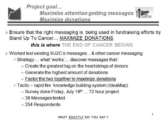
Figure 1: The introductory page to the project summary, showing the goals of the project, the timetable, and the tactics.

The process as described here followed the specifications of the Mind Genomics process [5-7]

The study proceeded very quickly. Author Onufrey worked with the SU2C team to create a set of 36 different messages. These messages are shown in Table 1. The rapid pace of the project (front to back in three days maximum) forced the creation of messages, followed by some polishing and then insertion into a matrix. Usually the groups comprise coherent questions and the series of such questions ‘tell a simple story.’ The virtually breakneck speed of message creation allowed for some polishing of the elements, improving the quality of the messages before the actual research. The messages required about four hours to develop, and two hours to polish. The field portion, with respondents, lasted a day and a half, and the report was finished the last night.

Table 1: The 36 elements for the study.

The conventional research approach would have been either to test these elements one-at-a-time (so-called promise testing), or to test a limited number of combinations created by the researcher or by a marketing specialist with a ‘sensibility of what the listener needs to hear to drive donation.’ These methods are hallowed in the research community because they introduce the ‘voice of the consumer.’

The reality of most research is that no one knows which elements will perform very well. It is fairly easy to spot losing elements, especially after the promise testing study is completed. These ‘losing’ elements may be adequate in and of themselves, but they don’t do well because they may be trite, or ‘off strategy.’ After the performance of each element, or the entire concept, is published for everyone to see, the opinions will emerge as to why the elements failed, alongside new and better elements.

The messages were combined by an underlying experimental design, creating 48 unique vignettes (combinations of messages), 36 comprising four elements (two questions not contributing), and the remaining 12 comprising 3 elements (three questions not contributing). The Mind Genomics experiment was set up so that the respondent was shown a vignette and had to assign two ratings, one for Question 1 dealing with probability of donating, and the second for Question 2, dealing with the amount to be donated.

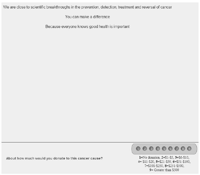
Figure 2: Example of a 3-element vignette, and rating question #2 (amount that would be donated, based upon reading the vignette).

To the untrained eye, and in fact even to someone who knows how the vignettes were developed, the combinations seem to be combined in a way that one might call constrainedly haphazard [8] All vignettes had a limited number of elements, and each element ended up appearing an equal number of times. The vignettes were created by a specially constructed experimental design, which was rotated to create hundreds of isomorphic permutations—combinations which were identical in a mathematical sense, but whose combinations were different.

These custom created experimental designs are the workhorses of Mind Genomics. They ensure that the respondent is exposed to each element the same number of times (five) in 48 vignettes, absent the same number of times (43), and that the 36 elements are statistically independent of other. The underlying experimental design ensured that each respondent evaluated a unique combination of 48 vignettes [9], and that each set of 48 vignettes suffices to estimate the contribution of each of the 36 elements both to propensity to donate (question #1) and amount expected to donate (question #2)

1. Probability of Donating – The first scale shows an anchored 1-9 scale, with the rating 1 anchored at ‘would not donate’ and the rating 9 anchored at ‘definitely would donate’. This is a Likert scale. It’s meaning is simple intuitively, but the scale must be anchored at both ends.
2. Amount donated – The second scale comprises nine numbers, each number corresponding to an amount of money. This second scale is easy to use.

To make the analysis easier, we converted the first scale (probability) of donating to nine values, ranging from a probability of 0% (original rating of 1, definitely not donate) to a probability of 100% (original rating of 9, definitely will donate). The nine points were considered to be equally spaced, so that a rating of 5, for example, was considered to be a probability of 50%, a rating of 6 a probability of 62.5% etc.

The first analysis looks at the distribution of ratings. Even before we look at the linkage between the different messages and donations (probability, amount, respectively), we can ask a simpler question, namely what is the relation between the probability of donating and the amount donated?

Table 2 shows a two-way cross tabulation. The numbers in the body of the table are the percent of times that the specific pair appears in the data (specific probability of donating, and amount donated).

Table 2: Distribution of probability of donating and amount donated. The numbers in the body of the table are percentages of all the responses.

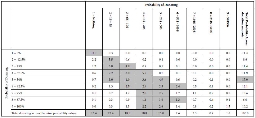
The far-right column in Table 2, labelled Total Probability, shows the distribution or probabilities of donating. Thus, 11.4% of the responses are ‘not donate,’ whether due to the respondents or to the messages. The source of the probability value is not clear. The most frequent response is ‘5’ (50% probability of donating), but that is only 17% of the responses. We can see that the percents not donating or donating (ratings 1-4) sum to 43% and the percents probably or definitely donating (ratings 6-9) total a bit over 40%,

The bottom row in Table 2, labelled Total Donating suggests, in contrast, that most donations are either 0 or less than 50$.

Is There a Discernible Relation between the Likelihood of Donating and Amount Donated?

Table 2 suggests that the relation between probability of donation and amount of donation exists, albeit in very rough and noisy form. Not surprisingly, there are more darkened cells towards the left side of the table, where the amount donated is lower, but there is not a correspondingly clearly shaded area when it comes to probability of donating.

We can create a less noisy data set by estimating the average donations and probability of donations for each of the 354 respondents. Figure 3 shows a plot of the averages, and suggests that with increasingly average likelihood of donating, there is a slight increase in the amount to be donated. The relation is noisy, however. It is clear, however, that when, on average the respondent is not interested in donating (low value of the abscissa), the respondent does not choose moderate to high amount of money to ‘not donate.’ This congruence of low donation probability and low/no donation amount, provides one indication of validity, in this case face validity. The pattern seems intuitively understandable.

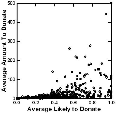
Figure 3: Relation between average rating of likely to donate and average amount to be donated. Each point is an average from 48 observations. There are 354 averages, one for each respondent.

Do Respondents Change Their Ratings as They Continue Rating Vignettes?

In the research community, and especially among applied research in a business setting, there is the ongoing dispute about the change in the criteria of judgment a respondent uses when judging a concept (vignette) or a product several times. Of course the concept or the product should be changed, but one can measure the effect of putting the concept or the product in the first position, the middle positions, or the last position. There is no end to the disputes about biases proposed by the purists who feel that every applied test of this type should be evaluated purely by itself, so-called pure monadic. There are others who feel that only with repeated experience does the respondent become able to validly rate the product. If the researcher relies only on the pure monadic, there is a great deal of extraneous variability, due to the proclivities and biases of the individual respondents.

The Mind Genomics approach attracts interest because the typical respondent evaluates as many as 24-48 vignettes, in short period of time, and without much consideration. The point of view espoused by a number of researcher is one of questioning the consistency of the data with repeated evaluations [10-14].

One of the analyses presented here looks at the change of the rating assigned by a respondent as the evaluations proceed from the first to the 48^th. Independent of the specific elements in a vignette, can we demonstrate a systematic bias, viz. that the average rating of the probability of donating will increase with repeated rating, or the amount given will increase with repeat rating?

Figure 4 shows an order ‘effect, both in terms of probability (likelihood) of donating (left panel), and amount of money to be donated (right panel). The two plots were created simply by averaging the rated likelihood to donate by ‘test order,’ and amount to be donated, also by ‘test order.’ For both likelihood and probability to donate, and for amount to donate, we see the upward pattern, suggesting that as the evaluations move on, respondents feel more generous. Respondents may not realize that they are being more generous, and the degree of generosity is not marked, but there is a noticeable increase.

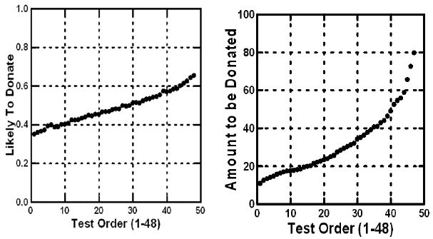
Figure 4: Average probability of donating (question #1) and average amount to be donated (question #2) versus the test order. Later vignettes are uprated on both ratings.

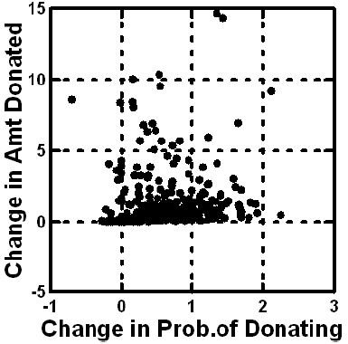
The foregoing analysis shown in Figure 3 suggests that on average, individuals become increasingly generous in terms of both likelihood and probability of donating, and amount to be donated. Does this pattern hold for the average individual? The slopes of the curves in Figure 3 provide us the answer. What does this slope look like on an individual basis? The answer appears in Figure 4. Each point corresponds to a respondent. The slopes were computed separately for the data of each respondent. Figure 5 shows the two slopes on a scatterplot. Slopes near zero mean no change. High positive slopes mean a strong positive increase in the rating with repeated evaluation. Negative slopes mean a decrease in the rating with repeated evaluation.

We conclude from Figure 4 that repeating the evaluation 48 times with new combinations ends up increasing the stated likelihood to donate, and the amount to be donated. The strength of the effect (slope) varies by respondent to respondent. There is only one respondent who strongly decreases the amount donated and the probability of donation, as the respondent progresses. Most respondents fall into the right half, and the top half, suggesting either a modest increase in probability of donating (to the right on the abscissa), or a modest increase in the amount to be donated (upwards on the ordinate). There is no clear pattern, however. As the person moves through the 48 vignettes, evaluating each, the person might increase the rated probability of donating, increase the rated amount to be donated, increase both, or increase neither.

Relating the Elements to the Ratings

Most research works with numbers to identify patterns. The preliminary, viz., surface analysis of the data, shown in Table 2 and Figures 3-5 tell us a lot about the respondent, in terms of likelihood to donate, response to repeated messages, etc. Yet, the deepest information is yet to be obtained, information which can only emerge when the stimuli are ‘cognitively rich.’

Figure 5: Distribution of changes in likelihood of donating (abscissa) and amount to be donated (ordinate), as shown by the slopes (versus test order). Numbers above 0 mean an increase in the likelihood or donating or the amount to be donated. Each point corresponds to one of the respondents.

Table 1 shows the 36 elements, with the underlying experimental design combining these elements into vignettes which communicate information about the efforts of SU2C. Table 2 shows us that respondents differentiate among these different vignettes. Beyond the effects of order, the underlying experimental design allows us to uncover the linkage between the specific element and the rating, either of probability to donate or amount to be donated.

The tool to be used is OLS (ordinary least-squares) regression analysis. OLS works regression with the underlying experimental design, deconstructing the rating assigned to the combination into the part-worth contributions of the elements. The experimental design was applied separately create the set of 48 vignettes for each respondent, allowing OLS regression to estimate, at either the level of the respondent or the level of the group, the part-worth contribution of each element.

We express the relation between the dependent variable and the independent variable by the simple equation: Dependent Variable = k₀ +k₁(A1) + k₂(A2) … k₃₆(F6)

The foregoing equation is easy to interpret. The equation for the dependent variables begins with an additive constant, k₀, which is the estimated value of the dependent variable when there are no elements in the vignettes. This situation is purely hypothetical because the underlying experiment ensured that EACH vignette created would have a precise set of either three elements or four elements, respectively. The additive constant, k₀, can thus be considered to be a baseline, the estimated value of the dependent variable without any other information.

1. Probability of donating – the baseline likelihood to donate to SU2C in the absence of any elements.
2. Estimated amount donate – the baseline amount that would be donated to SU2C, in the absence of any elements.
3. Expected value – the ‘adjusted’ amount that would be donated, defined as the amount to be donated, multiplied by the probability of the donation, again in the absence of any elements.

The OLS regression requires preparation of the data so that all of the data are in the proper format. The 36 independent variables, on for each elements, are coded as ‘1’ when the element is present in the vignette, and coded ‘0’ when the element is absent from the vignette. For statistical validity, the OLS regression approach requires more observations (viz., vignettes) than there are independent variables. Each respondent was presented with 36 independent variables, viz. our 36 elements, taking on the value 0 (absent) or 1 (present), and contributed 48 such cases or observations to the data set. Even at the level of the individual respondent, therefore, the OLS regression will run, delivering the coefficients.

As a side note, the study used three dependent variables. Each value was ‘adjusted’ by the additional of a very small random number (<10^-5), ensuring that there would be some slight variation in the dependent variable, and thus prevent a crash if the respondent assigned the same rating to each of the 48 vignette. This done not happen very often, but it is always better to add a bit of random variation to the dependent variable and prevent crashes.

We now move to the actual data itself, with the equations estimated using the data from the entire panel. Despite the apparent blooming buzzing confusion, a phrase that one might use to describe the person’s reaction to the vignettes, the results emerge quite clearly, or if not clearly, at least tell a story.

Table 3 shows two sets of three models—parameters for the equations. The first set is computed using all 36 elements, and estimating the additive constant, and the value of the individual coefficients. We can liken this first set of equations (columns A, B, and C) to a statue comprising two parts, a base, and then the statue part. The additive constant is the base, and the 36 elements are the parts of the statue. The height of the statue is estimated by adding together the magnitude of the additive constant and the coefficients of the particular, limited number of elements to be incorporated into a new vignette.

Table 3: The part-worth contribution of each of the elements to donations. The table shows the contributions when the model is estimated with an additive constant (baseline), and when the model is estimated without an additive constant (no baseline).

In contrast to the estimates of the coefficients in a model with an additive constant, we can choose to leave out the additive constant. Columns D, E, and F show the corresponding (and much larger) coefficients. Figure 6 shows, however, that there is little loss of relative information. The corresponding pairs of coefficients (viz., A & D, for probability of donating) are very highly related to each other, as are the other two corresponding pairs. Figure 6 shows the strong correlation.

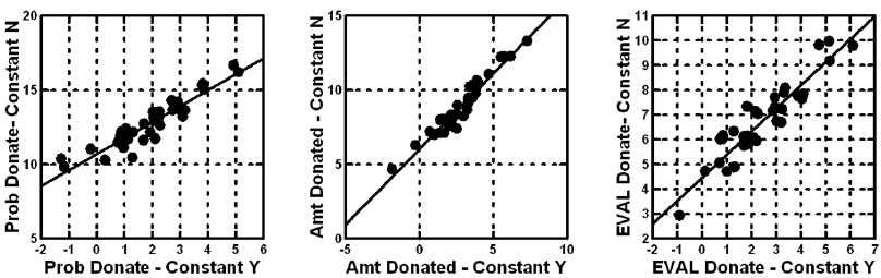
Figure 6: Scatterplots for each of the three dependent variables, showing the strong correlation between the 36 coefficients estimated with an additive constant (abscissa), and the 36 coefficients estimated but without an additive constant (ordinate).

Equations with the additive constant are estimated for those cases when there is a sense of a baseline ‘feeling,’ in the absence of elements. The judgments made based on the coefficients will be the same, because they line up so strongly in the same way.

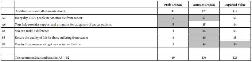
Table 4 makes it easy for managers to understand what is working. We need only sort the table to find those elements which generate high probabilities of donating, and/or high amounts of donated money, and/or high expected value.

Table 4 shows us that the additive constant for probability of donating is a base of 41%. The two elements which drive donation most strongly, here operationally defined as an addition 5%, are A3 and A6. In turn the additive constant for amount to be donated ins 23$ in the absence of elements. One can get an addition 6-7 dollars, however by the correct choice of elements. Finally, when we look at the expected value, combining probability and amount, we end up with an additive constant of 17$. Looking across Table 4, the manager of the campaign would be advised to choose combination of A3 and B2.

Table 4: Strong performing elements for the three dependent variables, and the recommended combination.

The Allure of Mind-Sets

A continuing theme in Mind Genomics is the discovery of underlying groups of respondents, distinguished not so much by WHO they are, but by how they think. Marketers call these psychographic segments. The segments are typically created on the basis of variables such as age, gender, geography. These geo-demographic variables are relative blunt measures, because people who resemble each other in their geo-demographics often think in radically different ways. One need only visit a neighborhood food store to see the array of different flavors of the same food, sold to people of similar geo-demographic profiles.

A better way is to discover how people think about a topic. There are various approaches for identifying groups of people, who are demonstrated to think differently on a set of related topics such as lifestyle. The problem with these methods of dividing the population is that the methods come from the top down, showing differences in the way people think about large topics. How does one translate membership in a big lifestyle segment to the exact words one needs to use for a targeted campaign, with limited focus, and even more limited budget?

Mind Genomics works from the bottom-up, creating mind-sets or groups of people, based exclusively on the patterns of their reactions to the important stimuli, namely the messages. The key benefit provided by Mind Genomics is the ability to create an equation or model for each respondent, based upon the responses to the 48 vignettes. One can then cluster the 354 respondents based upon the pattern of the coefficients. The actual clustering method is left to the researcher.

Mind Genomics follows a simple process to discover mind-sets.

1. Run three parallel analyses, one for each dependent variable; probability of donating, amount donated, expected value. The clustering analysis was thus done three times, once for each dependent variable.
2. Choose the dependent variable (e.g., Probability of Donating). For the chosen dependent variable create the 354 individual level models, using OLS regression. For this specific study on messaging, the models were estimated without an additive constant. As Figure 6 shows, the same pattern of coefficients appears whether the researcher incorporates or does not incorporate the additive constant.
3. Cluster the 354 respondents based upon the respondents’ patterns of coefficients, created using k-means clustering (Likas et. al., 2003). Individuals with similar patterns of 36 coefficients were put into the same cluster. The cluster will become the ‘mind-set’.
4. Extract three clusters of mind-sets and assign each of the 354 respondent to the appropriate mind-set.
5. Note that when we do the foregoing exercise three times, once for each dependent variable, the composition of the three mind-sets will change. That is, the composition of the three mind-sets or clusters, differs by the dependent variable.
6. The foregoing steps have now created three new groupings for every dependent variable. These groups are the mind-sets. For every dependent variable, every one of the 354 respondents is assigned to exactly one of the three mind-sets.

Now, consider one dependent variable, e.g., probability of donating. Each respondent fits into only one of the three mind-sets. We analyze the data on a mind-set basis.

1. Compute the average rating (or expected value) for each mind-set across all the respondents in the mind-set and all the 48 vignettes for each respondent. This average gives a sense of how the mine-set feels about the topic.
2. Once again, run the equation for the dependent variable selected (viz., Probability of Donating, dependent variable 1). This time, estimate the equation using the additive model. Run the OLS regression analysis three times, once incorporating all the data from the respondents assigned to the mind-set for that dependent variable.
3. Lay out the result and select only the strong-performing elements for each mind-set. The definition of ‘strong performing’ is a coefficient above a certain cutoff. The cutoff is operationally specified by the researcher.
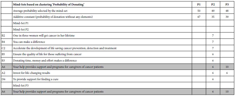
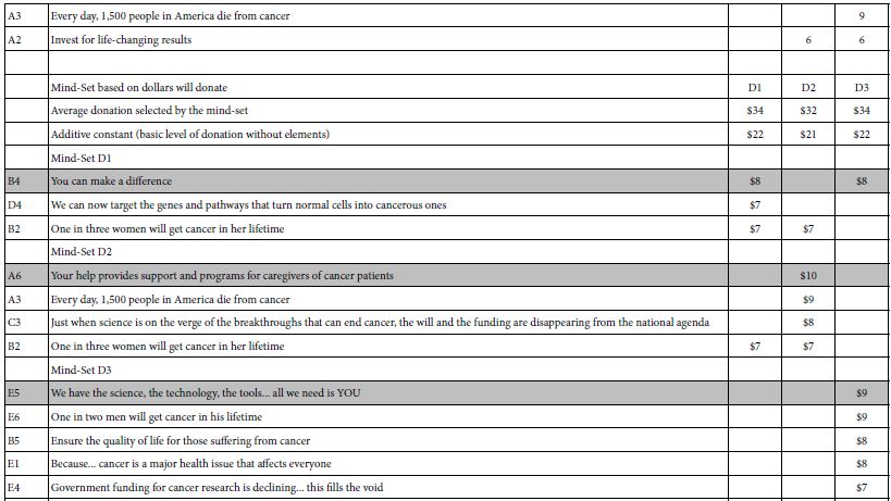
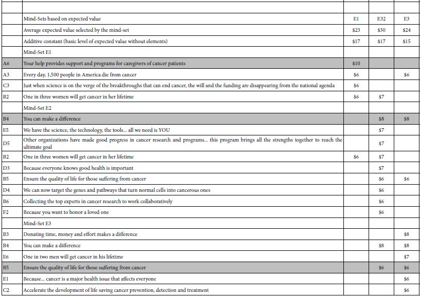
4. If an element fails to perform strongly for all three mind-sets, then eliminate the element. This action will eliminate most of the elements, allowing only the most promising elements. These are elements which do well for at least one mind-set. Tables 5shows the strong performing elements for each of the three mind-sets for a dependent variable.
5. For purposes of selecting the correct messages for the proposed SU2C, Table 5 presents the relevant information from which to craft messages.
6. For systematized understanding and data-basing in a ‘wiki of the mind,’ the original motivation for this reanalysis of the data 13 years later, Table 5 present the necessary information to better understand the mind of the donor, and to create a Mind Genomics of donation.

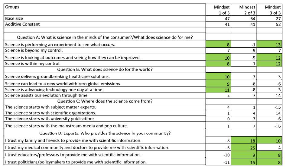
Table 5: Summary results for three mind-sets emerging for each dependent variable, and the strong performing elements for each mind-set. The recommended messages to use are shown in shaded cells.

Discussion and Conclusions

At the time of writing Selling Blue Elephants (2006 for the 2007 publication deadline), the realization emerged that one could do studies for companies and other groups, studies which would answer the question, but studies which would have great residual value. It was in this spirit that many studies were run, studies which created these so-called rules. The question then was asked: Can these studies be reopened a significant time later, when the issue had been long answered, and in turn, can these studies ‘teach.’ If so, the opportunity was emerging to create studies whose value would be immediate AND long term. It is to that issue that we addressed this paper, with a case history about what was done, and what was learned 13 years later of a general nature.

By their very nature, Mind Genomics study provides valuable information years, even decades after they have been executed. The reason for the retained value is two-fold. First, the raw material, the elements, is cognitively rich. A database of the type shown in Tables 4 and 5 but comprising all 36 elements rather than just ‘strong performers’, becomes a valuable. The database can be searched, and new facts and insights can be discovered. One can imagine a world where there are millions or even hundreds of millions of these databases created each year, and available for search to broaden our understanding. The result is a Wikipedia of the Mind, produced at the level of local issues, at the level of granularity.

There is a second use, as well. That is as a database from which one can extract meta-patterns, such as average ratings of subgroups, or change in response patterns over time. This second use pales, of course, when compared to the first application above, the Wikipedia of the Mind at the level of granular, everyday experience. Yet, when we emerge from the euphoria of what could be, we realize that it is this less-exciting second use which corresponds to today’s archival sciences. Information, but without the systematized, cognitive richness so readily available from Mind Genomics.

The final question is very simple. Was the study effective? Here is a direct quote from 2010. Although one might not attribute the massive success of SU2C, the fact that those running the simulcast in 2008 knew ‘what to say’ should be taken into account as a factor in the success of SU2C, in its effort to change the perception of cancer, and to highlight the efforts being made to treat it, control it, and cure it.

Stand Up to Cancer

LOS ANGELES—A look at some of the statistics culled from the Stand Up to Cancer (SU2C) Sept. 10 broadcast may seem to indicate that the fundraising and cancer awareness effort fell somewhat short of its original milestones two years before: The 2010 show announced that $80 million had been pledged, whereas in 2008 the number was approximately $100 million. ….

The first show was seen on only ABC, CBS, and NBC, which for this year’s show were joined by many more collaborative network and cable partners including Fox, Bio, Current TV, Discovery Health, E!, G4, HBO, HBO Latino, MLB Network, mun2, Showtime, Smithsonian Channel, the Style Network, TV One, and VH1…..(Source… [11]).

References

1. Moskowitz HR, Gofman A (2007) Selling Blue Elephants: How to Make Great Products That People Want Before They Even Know They Want Them. Pearson Education.
2. Christen SP, Levine AJ (2019) Facilitating cross-disciplinary interactions to stimulate innovation: Stand Up To Cancer’s matchmaking convergence ideas lab. In Strategies for Team Science Success. Springer.
3. Charlesworth D (2016) Stand Up to Cancer 2012 and 2014: The medical telethon as UK public service broadcasting in a neo-liberal age. Critical Studies in Television 11: 217-229.
4. Gabay G, Moskowitz H, Gere A (2019) Understanding the donating mind and optimizing messaging – public hospitals. In: 12th Annual Conference of the EuroMed Academy of Business.
5. Gere A, Radvanyi D, Moskowitz H (2017) The Mind Genomics metaphor – from measuring the every-day to sequencing the mind. International Journal of Genomic Mining.
6. Mehta-Shah N, Mehta S, Zemel R (2021) Mind Genomics (BimiLeap) to create new ideas. In Consumer-based New Product Development for the Food Industry. Royal Society of Chemistry 119-131.
7. Moskowitz HR, Gofman A, Beckley J, Ashman H (2006) Founding a new science: Mind Genomics. Journal of Sensory Studies 21: 266-307.
8. Ryan TP, Morgan JP (2007) Modern experimental design. Journal of Statistical Theory and Practice 1: 501-506.
9. Gofman A, Moskowitz H (2010) Isomorphic permuted experimental designs and their application in conjoint analysis. Journal of sensory studies 25: 127-145.
10. Schwarz N, Hippler HJ, Noelle-Neumann E (1992) A cognitive model of response-order effects in survey measurement.” In Context Effects in Social and Psychological Research. Springer 187-201.
11. Rosenthal ET (2010) Stand Up to Cancer 2010: Qualitative Success Transcends Quantitative Numbers Oncology Times 32: 20-23.
12. Fortunato J (2013) Sponsorship activation and social responsibility: How MasterCard and major league baseball partner to stand up to cancer. Journal of Brand Strategy 2: 300-311.
13. Likas A, Vlassis N, Verbeek J (2003) The global k-means clustering algorithm. Pattern Recognition, Elsevier 36: 451-461.
14. Milutinovic V, Salom J (2016) Mind Genomics: A Guide to Data-Driven Marketing Strategy. Springer.

DOI: 10.31038/CST.2021631

Abstract

Uterine leiomyomas are the most common gynecological tumors in women of reproductive age. However, there are cases of atypical localization, which could represent a diagnosis and treatment challenge. We describe the case of a 54-year-old female patient, with the finding of a large intra-abdominal mass, compatible with gynecological-type leiomyoma, located at the upper retroperitoneum, successfully diagnosed and treated with laparoscopic surgery.

Keywords

Retroperitoneal tumors, Ginecologic-type leiomyoma, Surgery, Laparoscopic surgery

Introduction

Uterine leiomyomas (also called myomata or fibroids) are the most common pelvic neoplasms in women [1,2]. They arise from the smooth muscle cells of the myometrium and extrauterine locations are extremely rare. Although they are histologically benign, in the presence of an atypical presentation, they could mimic malignant tumors at imaging and may become a diagnostic and treatment challenge that will require a multidisciplinary approach [3,4].

The case of a 54-year-old female patient, diagnosed with a large intra-abdominal mass, compatible with gynecological-type leiomyoma, located at the upper retroperitoneum, is presented.

Case Presentation

A 54-year-old female patient, with a history of hysterectomy for uterine fibroids, was diagnosed with an asymptomatic giant retroperitoneal mass, detected by ultrasound, as part of medical follow-up. In order to better assess this finding, a Magnetic Resonance Image (MRI) was carried out showing a left retroperitoneal lesion of 142 x 88 x 86 mm, of probable mesenchymal origin, causing displacement of the splenic vein, tail of the pancreas, kidney and spleen, with no clear dependence on any organ (Figure 1A and 1B).

Figure 1: MRI (A: Axial and B: coronal views) showing an heterogeneous retroperitoneal mass of 142 x 88 x 86 mm.

The case was discussed on a multidisciplinary committee and based on the size and unknown origin of the lesion, she was considered a candidate for resection. The patient was placed in a lateral decubitus position and a laparoscopic approach was performed. Retroperitoneum was accessed by previously dissecting the sigmoid colon in a lateral to medial fashion. After identification of the mass, a complete resection was performed emphasising not to open the tumor´s capsule (Figure 2). The postoperative course was uneventful and the patient was discharged on the third postoperative day. Pathological analysis of the resected specimen revealed a nodular lesion constituted by a proliferation of elongated, fusiform cells of typical  muscle appearance without marked mitotic activity (<1 mitosis in 50 HPF) (Figure 3A). Hormonal receptors (Estrogen and Progesterone) showed intense and diffuse positivity (Figure 3B). These findings are consistent with gynecologic type retroperitoneal leiomyoma.

Figure 2: Laparoscopic image showing retroperitoneal mass (black arrow), sigmoid colon (yellow asterisk), left kidney (green asterisk) (A, B and C). After complete dissection, the extraction was performed in a protective bag through a pfannenstiel incision (D).

Figure 3: A: Gynecologic-type leiomyoma of retroperitoneum. Hematoxylin-Eosin (H-E) staining sections show intersecting fascicles of slender tapered smooth muscle cells arranged in a whorled pattern separated by well vascularized connective tissue. B: Gynecologic-type leiomyoma of retroperitoneum. Estrogen receptor protein (ER) nuclear staining shows irregular packets and fascicles of spindle cells.

Discussion

Leiomyomas represent the most common gynecologic and uterine neoplasms, diagnosed in up to 70% of women during their lifetime [5]. They originate primarily from smooth muscle cell proliferation in the myometrium and extrauterine locations are extremely rare [6]. Although they are histologically benign, extrauterine leiomyomas may mimic malignant tumors at imaging and may become a diagnostic challenge [6,7].

Analyzing the differential diagnoses to be taken into account when facing a retroperitoneal mass, a wide range of tumors can be found, both benign and malignant. Generally, they are divided into solid or cystic, based on the different imaging modalities [8]. In turn, each subgroup is subdivided into neoplastic and non-neoplastic [9,10]. The real incidence of each of these pathologies is unknown [11]. However, it has been shown that 80% of primary retroperitoneal neoplasms are malignant [12]; in fact the retroperitoneal space is the second most frequent location, followed by the lower extremities, where malignant mesenchymal tumors arise. Approximately, one third of retroperitoneal tumors are sarcomas [13]. The most frequent sarcomas are liposarcoma, malignant fibrous histiocytoma, and leiomyosarcoma [14,15]. Given that treatment options vary, it is useful to be able to noninvasively distinguish these masses, this is why preoperative imaging including MRI must be performed [16]. Nevertheless, is a fact, that most of the times it will not be possible to define the tumor`s nature [17]. Due to the lack of diagnostic accuracy, using currently available radiologic modalities, prompt surgical intervention will usually be indicated; more if we take into account that these tumors are usually asymptomatic and they may become huge masses before diagnose.

A laparoscopic approach is technically feasible and safe, and should be considered for this cases, given the well described advantages of this approach such as less postoperative pain, rapid recovery, and better cosmetic results [10,18]. However, the size and location could potentially be factors to hinder laparoscopic feasibility. If adequate safety margins cannot be ensured, and risk of opening the tumor´s capsule is present, an open procedure should be performed [19].

Conclusion

The relevance of the present case lies in the unusual presentation of a gynecologic type leiomioma as a retroperitoneal mass. As mentioned before, it must be taken into account in the differential diagnosis of retroperitoneal masses, especially when the patient has a history of leiomyoma.

Acknowledgments

The authors would like to thank the pathology department of the Hospital Italiano de Buenos Aires, for their services.

Conflicts of Interest

The authors declare not having any conflicts of interest.

Ethical Disclosures

Protection of Human and Animal Subjects

The authors declare that no experiments were performed on humans or animals for this study.

Confidentiality of Data

The authors declare that they have followed the protocols of their work center on the publication of patient data.

Right to Privacy and Informed Consent

The authors have obtained the written informed consent of the patients or subjects mentioned in the article. The corresponding author is in possession of this document.

References

1. Stewart EA, Cookson CL, Gandolfo RA, Schulze-Rath R (2017) Epidemiology of uterine fibroids: a systematic review. BJOG: An International Journal of Obstetrics & Gynaecology 124: 1501-1512. [crossref]
2. Victory R, Romano W, Bennett J, Diamond MP (2015) Uterine leiomyomas: epidemiology, diagnosis, and management. Clinical Gynecology 223-252.
3. Fasih N, Shanbhogue AKP, Macdonald DB, Fraser-Hill MA, Papadatos D, et al. (2008) Leiomyomas beyond the uterus: Unusual locations, rare manifestations. Radiographics 28: 1931-1948. [crossref]
4. Poliquin V, Victory R, Vilos GA (2008) Epidemiology, Presentation, and Management of Retroperitoneal Leiomyomata: Systematic Literature Review and Case Report. Journal of Minimally Invasive Gynecology 15: 152-160. [crossref]
5. Giuliani E, As-Sanie S, Marsh EE (2020) Epidemiology and management of uterine fibroids. J. Gynaecol. Obstet 149: 3-9. [crossref]
6. Chin H, Ong XH, Yam PKL, Chern BSM (2014) Extrauterine fibroids: a diagnostic challenge and a long-term battle. BMJ Case Rep 2014: 2014204928. [crossref]
7. Takeda T, Asaoka D, Fukumura Y, Watanabe S (2017) Asymptomatic giant retroperitoneal mass detected at a medical checkup. Clin Case Rep 5: 2148-2150. [crossref]
8. Rajiah P, Sinha R, Carlos C, Dubinsky TJ, Bush WHJ, et al. (2011) Imaging of Uncommon Retroperitoneal Masses. RadioGraphics 31: 949-976. [crossref]
9. Osman S, Lehnert BE, Elojeimy S, Cruite I, Mannelli L, et al. (2013) A Comprehensive Review of the Retroperitoneal Anatomy, Neoplasms, and Pattern of Disease Spread. Current Problems in Diagnostic Radiology 42: 191-208. [crossref]
10. Wee-Stekly WW, Mueller MD (2014) Retroperitoneal Tumors in the Pelvis: A Diagnostic Challenge in Gynecology. Frontiers in Surgery 1: 49.
11. Scali EP, Chandler TM, Heffernan EJ, Coyle J, Harris AC, et al. (2015) Primary retroperitoneal masses: what is the differential diagnosis? Abdom Imaging 40: 1887-1903. [crossref]
12. Neville A, Herts B (2004) CT Characteristics of Primary Retroperitoneal Neoplasms. Critical Reviews in Computed Tomography 45: 247-270. [crossref]
13. Clark MA, Fisher C, Judson I, Meirion Thomas J (2005) Soft-Tissue Sarcomas in Adults. New England Journal of Medicine 353: 701-711.
14. Francis IR (2005) Retroperitoneal sarcomas. Cancer Imaging 5: 89-94.
15. Gupta AK, Cohan RH, Francis IR, Sondak VK, Korobkin M (2000) CT of Recurrent Retroperitoneal Sarcomas. American Journal of Roentgenology 174: 1025-1030. [crossref]
16. Shah JD, Kirshenbaum M, Shah KD (2008) CT Characteristics of Primary Retroperitoneal Tumors And the Importance of Differentiation From Secondary Retroperitoneal Tumors. Contemporary Diagnostic Radiology 31: 1-5.
17. Fasih N, Shanbhogue AKP, Macdonald DB, Fraser-Hill MA, Papadatos D, et al. (2008) Leiomyomas beyond the Uterus: Unusual Locations, Rare Manifestations. RadioGraphics 28: 1931-1948. [crossref]
18. Tsivian M, Ami Sidi A, Tsivian A (2009) Laparoscopic Management of Retroperitoneal Masses: Our Experience and Literature Review. World Journal of Laparoscopic Surgery with DVD 1-5.
19. Cadeddu MO, Mamazza J, Schlachta CM, Seshadri PA, Poulin EC (2001) Laparoscopic Excision of Retroperitoneal Tumors. Surgical Laparoscopy, Endoscopy & Percutaneous Techniques 11: 144-147. [crossref]

References

1. Reardon S (2015) Ebola’s mental-health wounds linger in Africa: Health-care workers struggle to help people who have been traumatized by the epidemic. Nature 519: 13-15. [crossref]
2. Shin J, Park HY, Kim JL, Lee JJ, Lee H, et al. (2019) Psychiatric Morbidity of Survivors One Year after the Outbreak of Middle East Respiratory Syndrome in J Korean Neuropsychiatr Assoc 58: 245-251.
3. Lee AM, Wong JG, McAlonan GM, Cheung V, Cheung C et al. (2007) Stress and Psychological Distress among SARS Survivors 1 Year after the Can J Psychiatry, 52: 233-240. [crossref]
4. Garcia R (2017) Neurobiology of fear and specific phobias. Learn Mem 24: 462-471. [crossref]
5. Shin LM, Liberzon I (2010) The neurocircuitry of fear, stress, and anxiety disorders. Neuropsychopharmacology 35: 169-191. [crossref]
6. Shigemura J, Ursano RJ, Morganstein JC, Kurosawa M, Benedek DM (2020) Public responses to the novel 2019 coronavirus (2019-nCoV) in Japan: mental health consequences and target populations. Psychiatry Clin Neurosci 74: 281-282. [crossref]
7. Kim, J (2020) Clinical Feature of Coronavirus Disease 2019 in Elderly. Korean J Clin Geri 21: 1-8.
8. Wang C, Pan R, Wan X, Tan Y, Xu L (2020) Immediate Psychological Responses and Associated Factors during the Initial Stage of the 2019 Coronavirus Disease (COVID-19) Epidemic among the General Population in China. Int J Environ Res Public Health, 17.
9. Brooks SK, Webster RK, Smith LE, Woodland L, Wessely S, et al. (2020) The psychological impact of quarantine and how to reduce it: rapid review of the evidence. Lancet. 395: 912-920. [crossref]
10. Gerst-Emerson K, Jayawardhana J (2015) Loneliness as a Public Health Issue: The Impact of Loneliness on Health Care Utilization Among Older Adults. Am J Public Health 105: 1013-1019. [crossref]
11. Xiang YT, Yang Y, Li W, Zhang L, Zhang Q, Cheung T et al. (2020) Timely mental health care for the 2019 novel coronavirus outbreak is urgently needed. Lancet Psychiatry 7: 228-229. [crossref]
12. Maunder R, Hunter J, Vincent L, Bennett J, Peladeau N, Leszcz M et al. (2003) The immediate psychological and occupational impact of the 2003 SARS outbreak in a teaching hospital. CMAJ 168: 1245-1251. [crossref]
13. Shigemura J, Ursano RJ, Morganstein JC, Kurosawa M, Benedek DM (2020) Public responses to the novel 2019 coronavirus (2019-nCoV) in Japan: mental health consequences and target populations. Psychiatry Clin Neurosci 74: 281-282. [crossref]
14. One in 5 COVID-19 patients develop mental illness within 90 days – study. Reuters. 10 November 2020.
15. Flaviane CristineTroglio da Silva, Caio ParenteBarbosa (2021) THE IMPACT OF THE COVID-19 PANDEMIC IN AN INTENSIVE CARE UNIT (ICU): PSYCHIATRIC SYMPTOMS IN HEALTHCARE PROFESSIONALS – A SYSTEMATIC REVIEW. Journal of Psychiatric Research. March 25.
16. Huang JZ, Han MF, Luo TD, Ren AK, Zhou XP (2020) [Mental health survey of 230 medical staff in a tertiary infectious disease hospital for COVID-19]. Zhonghua Lao Dong Wei Sheng Zhi Ye Bing Za Zhi 38: 192-195. [crossref]
17. Kang L, Li Y, Hu S, Chen M, Yang C, et al. (2020) The mental health of medical workers in Wuhan, China dealing with the 2019 novel coronavirus. Lancet Psychiatry [crossref]
fig 2
Huge Retroperitoneal Mass: Ginecologic-Type Leiomyoma
1. Cancer (2012, September 8) World Health Organization. https://www.who.int/news-room/fact-sheets/detail/cancer.
2. Cancer costs projected to reach at least $158 billion in 2020 (2011, January 11) National Institutes of Health (NIH). https://www.nih.gov/news-events/news-releases/cancer-costs-projected-reach-least-158-billion-2020
3. Cancer Facts & Figures 2018 | American Cancer Society. (2018) Cancer Facts & Figures 2018. https://www.cancer.org/research/cancer-facts-statistics/all-cancer-facts-figures/cancer-facts-figures-2018.html
4. Cancer Prevention Overview (PDQ®)–Patient Version—National Cancer Institute (nciglobal,ncienterprise) (2009, June 22) [PdqCancerInfoSummary]. https://www.cancer.gov/about-cancer/causes-prevention/patient-prevention-overview-pdq
5. CDC – Expected New Cancer Cases and Deaths in 2020 (2019, January 31). https://www.cdc.gov/cancer/dcpc/research/articles/cancer_2020.htm
6. Hanrahan, L. P., Anderson, H. A., Busby, B., Bekkedal, M., Sieger, T., Stephenson, L., Knobeloch, L., Werner, M., Imm, P., & Olson, J (2004) Wisconsin’s Environmental Public Health Tracking Network: Information Systems Design for Childhood Cancer Surveillance. Environmental Health Perspectives 112(14), 1434–1439. https://doi.org/10.1289/ehp.7150 [crossref]
7. History of the Cancer Prevention Studies. (n.d.). American Cancer Society. Retrieved October 7, 2019, from https://www.cancer.org/research/we-conduct-cancer-research/behavioral-and-epidemiology-research-group/history-cancer-prevention-study.html
8. Humans, I. W. G. on the E. of C. R. to. (2010) Summary of Data Reported. In Alcohol Consumption and Ethyl Carbamate. International Agency for Research on Cancer. https://www.ncbi.nlm.nih.gov/books/NBK326555/ [crossref]
9. Late-stage cancer detection in the USA is costing lives—The Lancet (2010, December 4). The Lancet. https://www.thelancet.com/journals/lancet/article/PIIS0140-6736(10)62195-2/fulltext
10. Limit Alcohol Consumption. (n.d.). American Institute for Cancer Research. Retrieved October 7, 2019, from https://www.aicr.org/cancer-prevention/recommendations/limit-alcohol-consumption/
11. Moolgavkar, S. H., Holford, T. R., Levy, D. T., Kong, C. Y., Foy, M., Clarke, L., Jeon, J., Hazelton, W. D., Meza, R., Schultz, F., McCarthy, W., Boer, R., Gorlova, O., Gazelle, G. S., Kimmel, M., McMahon, P. M., de Koning, H. J., & Feuer, E. J (2012) Impact of Reduced Tobacco Smoking on Lung Cancer Mortality in the United States During 1975–2000. JNCI Journal of the National Cancer Institute 104(7), 541–548. https://doi.org/10.1093/jnci/djs136
12. Nelson, D. E., Jarman, D. W., Rehm, J., Greenfield, T. K., Rey, G., Kerr, W. C., Miller, P., Shield, K. D., Ye, Y., & Naimi, T. S (2013) Alcohol-Attributable Cancer Deaths and Years of Potential Life Lost in the United States. American Journal of Public Health 103(4), 641–648. https://doi.org/10.2105/AJPH.2012.301199 [crossref]
13. Novello, A. C. (1990) Surgeon General’s report on the health benefits of smoking cessation. Public Health Reports 105(6), 545–548. [crossref]
14. Patel, A. V., Jacobs, E. J., Dudas, D. M., Briggs, P. J., Lichtman, C. J., Bain, E. B., Stevens, V. L., McCullough, M. L., Teras, L. R., Campbell, P. T., Gaudet, M. M., Kirkland, E. G., Rittase, M. H., Joiner, N., Diver, W. R., Hildebrand, J. S., Yaw, N. C., & Gapstur, S. M (2017) The American Cancer Society’s Cancer Prevention Study 3 (CPS-3): Recruitment, study design, and baseline characteristics. Cancer 123(11), 2014–2024. https://doi.org/10.1002/cncr.30561. [crossref]
15. Proctor, R. N (2012) The history of the discovery of the cigarette–lung cancer link: Evidentiary traditions, corporate denial, global toll. Tobacco Control 21(2), 87–91. https://doi.org/10.1136/tobaccocontrol-2011-050338.
16. Recommendations (2017, September) U. S. Preventive Services Taskforce. https://www.uspreventiveservicestaskforce.org/uspstf/topic_search_results?topic_status=P&category%5B%5D=15&type%5B%5D=5&searchterm=cancer+screening
17. Risk Factors: Infectious Agents – National Cancer Institute (nciglobal,ncienterprise) (2015, April 29) [CgvArticle]. https://www.cancer.gov/about-cancer/causes-prevention/risk/infectious-agents.
18. Rothman, Kenneth J (1998a) Case-Control Studies / Kenneth J. Rothman, Sander Greenland. In Modern epidemiology / Kenneth J. Rothman, Sander Greenland ; with 15 contributors (2nd ed., pp. 93–114). Lippincott-Raven.
19. Rothman, Kenneth J (1998b) Cohort Studies / Kenneth J. Rothman, Sander Greenland. In Modern epidemiology / Kenneth J. Rothman, Sander Greenland ; with 15 contributors (2nd ed., pp. 79–92). Lippincott-Raven.
20. Schütze, M., Boeing, H., Pischon, T., Rehm, J., Kehoe, T., Gmel, G., Olsen, A., Tjønneland, A. M., Dahm, C. C., Overvad, K., Clavel-Chapelon, F., Boutron-Ruault, M.-C., Trichopoulou, A., Benetou, V., Zylis, D., Kaaks, R., Rohrmann, S., Palli, D., Berrino, F., … Bergmann, M. M (2011). Alcohol attributable burden of incidence of cancer in eight European countries based on results from prospective cohort study. BMJ 342. https://doi.org/10.1136/bmj.d1584.
21. pdf. (n.d.). Retrieved June 7, 2020, from https://seer.cancer.gov/about/factsheets/SEER_Overview.pdf.
22. Site Recode—SEER Recodes. (n.d.). Surveillance, Epidemiology, and End Results Program. Retrieved October 7, 2019, from https://seer.cancer.gov/siterecode/icdo3_dwhoheme/index.html.
23. Torre, L. A., Siegel, R. L., Ward, E. M., & Jemal, A. (2016) Global Cancer Incidence and Mortality Rates and Trends—An Update. Cancer Epidemiology and Prevention Biomarkers 25(1), 16–27. https://doi.org/10.1158/1055-9965.EPI-15-0578 [crossref]
24. Ultraviolet (UV) radiation and skin cancer (2017, October 16). https://www.who.int/news-room/q-a-detail/ultraviolet-(uv)-radiation-and-skin-cancer. [crossref]
25. What Are the Risk Factors for Lung Cancer? | CDC (2019, November 18). https://www.cdc.gov/cancer/lung/basic_info/risk_factors.htm
26. WHO | Cancer prevention (2019) WHO; World Health Organization. http://www.who.int/cancer/prevention/en/
27. Why is early diagnosis important? (2015, April 2) Cancer Research UK. https://www.cancerresearchuk.org/about-cancer/cancer-symptoms/why-is-early-diagnosis-important
28. Worldwide cancer statistics (2019). Cancer Research UK. https://www.cancerresearchuk.org/health-professional/cancer-statistics/worldwide-cancer
fig 6
Utilization of Co-evaporation Technique for Enhancement the Solubility and Dissolution Rate of Etodolac
DOI: 10.31038/JPPR.2021422
Abstract
Etodolac (ETD), a member of non-steroidal anti-inflammatory drugs (NSAIDs), has a poor aqueous solubility. Long term administration of ETD causes severe gastrointestinal disturbances such as peptic ulcer and bleeding. The enhancement of its solubility and dissolution profile is expected to improve its bioavailability and reduce its side effects. In the present study, we tried to enhance the aqueous solubility and dissolution rate of ETD by two co-evaporation techniques. The first one is the formation of solid dispersion with different hydrophilic carriers, including polyethelene glycol (PEG 4000), polyvinyl pyrrolidones (PVP K25 and PVP K90) and urea. The second method is the formation of solid adsorbates using inert carriers such as avecil PH 101, bentonite and aerosil 200 as adsorbents. Co-evaporates were prepared at (1:1 w/w), (1:3 w/w) and (1:5 w/w) ETD to carrier ratios and the corresponding physical mixtures were also prepared. The solubility and dissolution studies of all formulations were measured. Moreover, the physicochemical properties of the modified co-evaporates were characterized using different techniques including, differential scanning calorimetry (DSC), infrared spectroscopy and X-ray diffractometry (XRD) analysis. The results showed that the co-evaporates exhibited higher dissolution rate than the corresponding physical mixtures and both showed higher dissolution rate than the unmodified drug. Increase polymer concentration led to increase in the dissolution rate of drug. Plus, the dissolution rate was enhanced by increasing the temperature of the dissolution medium. Avecil PH 101 exhibited the highest dissolution rate over all other polymers. Infrared studies showed no interaction between the drug and the investigated carrier. The DSC and XRD studies indicated the conversion of ETD to an amorphous state. The enhancement of the drug solubility may be attributed to the increase of drug surface area, the wettability, formation of hydrogen bonds and the conversion to amorphous state.
Keywords
Etodolac, Co-evaporate, Solubility, Dissolution rate, Solid dispersion, Adsorbate, Hydrophilic carriers
1. Guo Q, Qiang G, Yuxiang W, Dan Xu, Johannes N, Nathan J, et al., (2018) Rheumatoid arthritis: pathological mechanisms and modern pharmacologic therapies. Bone Research 6: 1-14.
2. Pareek, A, Nitin Chandurkar,Tenpe SR, Yeole PG (2014) research article Evaluation of anti-inflammatory activity of etodolac and colchicine combination in experimental animals. International Journal of Clinical Pharmacology and Therapeutics.
3. Harirforoosh S, W Asghar, F Jamali (2013) Adverse effects of nonsteroidal antiinflammatory drugs: an update of gastrointestinal, cardiovascular and renal complications. Journal of Pharmacy & Pharmaceutical Sciences 16: 821-847.
4. Khaleel NY, et al., (2011) Solubility and dissolution improvement of Ketoprofen by solid dispersion in polymer and surfactant using solvent evaporation method. International Journal of Pharmacy and Pharmaceutical Sciences 3: 431-435.
5. Buckley ST, Kerstin JF, Gert F, Martin B, et al., (2013) Biopharmaceutical classification of poorly soluble drugs with respect to “enabling formulations”. European Journal of Pharmaceutical Sciences 50: 8-16. [crossref]
6. Chaudhary V, Patel J (2013) Cyclodextrin inclusion complex to enhance solubility of poorly water soluble drugs: A review. International Journal of Pharmaceutical Sciences and Research 4.
7. Rasenack N, Müller BW (2002) Dissolution rate enhancement by in situ micronization of poorly water-soluble drugs. Pharmaceutical Research 19: 1894-1900. [crossref]
8. Chiou WL, Chen SJ, Athanikar N (1976) Enhancement of dissolution rates of poorly water‐soluble drugs by crystallization in aqueous surfactant solutions I: Sulfathiazole, prednisone, and chloramphenicol. Journal of Pharmaceutical Sciences 65: 1702-1704. [crossref]
9. Otsuka M, Ofusa T, Matsuda Y (1998) Dissolution improvement of water-insoluble glybuzole by co-grinding and co-melting with surfactants and their physicochemical properties. Colloids and Surfaces B: Biointerfaces. 10: 217-226.
10. Rascioni R (2016) Effect of particle size reduction and crystalline form on dissolution behaviour of nimesulide. Journal of Thermal Analysis and Calorimetry 123: 2213-2223.
11. Dhore PW, Vivek SD, Suprit DS, Yamini SB, Connor Mack, et al. (2017) Enhancement of the aqueous solubility and permeability of a poorly water soluble drug ritonavir via lyophilized milk-based solid dispersions. Pharmaceutical Development and Technology. 22: 90-102. [crossref]
12. Chokshi RJ, Hossein Z, Harpreet KS, Navnit HS, Waseem AM et al., (2007) Improving the dissolution rate of poorly water soluble drug by solid dispersion and solid solution—pros and cons. Drug Delivery 14: 33-45. [crossref]
13. Friedrich H, Bernd F, Karl K, Roland B et al., (2006) Dissolution rate improvement of poorly water-soluble drugs obtained by adsorbing solutions of drugs in hydrophilic solvents onto high surface area carriers. European Journal of Pharmaceutics and Biopharmaceutics 62: 171-177. [crossref]
14. Sharma D (2016) Solubility enhancement strategies for poorly water-soluble drugs in solid dispersions: A review. Asian Journal of Pharmaceutics (AJP): Free full text articles from Asian J Pharm 1.
15. Das SK, Abha Doshi, Bhagyashri Joshi, Vandana Wankhede, Jesal Doshi, et al., (2012) Solid dispersions: an approach to enhance the bioavailability of poorly water-soluble drugs. International Journal of Pharmacology and Pharmaceutical Technology. 1: 37-46.
16. Zayed G (2014) Dissolution Rate Enhancement of Ketoprofen by Surface Solid Dispersion with Colloidal Silicon Dioxide. Unique J. Pharm. and Bio. Sci 1: 33-38.
17. Biswal S, J Sahoo, PN Murthy, RP Giradkar, JG Avari (2008) Enhancement of dissolution rate of gliclazide using solid dispersions with polyethylene glycol 6000. AAPS PharmSciTech 9: 563-570. [crossref]
18. Balata G, M Mahdi, Rania AB (2011) Bakera, Improvement of solubility and dissolution properties of clotrimazole by solid dispersions and inclusion complexes. Indian Journal of Pharmaceutical Sciences. 73. [crossref]
19. Xie T, L.S. Taylor (2016) Improved release of celecoxib from high drug loading amorphous solid dispersions formulated with polyacrylic acid and cellulose derivatives. Molecular Pharmaceutics 13: 873-884.
20. Kuharski RA, Rossky PJ (1984) Solvation of hydrophobic species in aqueous urea solution: a molecular dynamics study. Journal of the American Chemical Society. 106: 5794-5800.
21. Saha R, et al., (2002) Solubility enhancement of nimesulide and ibuprofen by solid dispersion technique. Indian Journal of Pharmaceutical Sciences 64.
22. Lima,ÁA, et al. (2011) The use of solid dispersion systems in hydrophilic carriers to increase benznidazole solubility. Journal of Pharmaceutical Sciences 100: 2443-2451.
23. Thenmozhi K, Yoo YJ (2017) Enhanced solubility of piperine using hydrophilic carrier-based potent solid dispersion systems. Drug Development and Industrial Pharmacy 43: 1501-1509. [crossref]
24. Waghmare A, Pore Y, Kuchekar B (2008), Development and characterization of zaleplon solid dispersion systems: a technical note. Aaps Pharmscitech 9: 536-543.
25. Law S, Chiang C (1990) Improving Dissolution Rates of Griseofulivin by Deposition on Disintegrants. Drug Development and Industrial Pharmacy. 16: 137-147.
26. Ismail A, K Saleh, S Khalaf (2004) Preparation and evaluation of naproxen adsorbate as an attempt to improve drug dissolution characteristics. Drugs 9.
27. Chella N, N Shastri, RR Tadikonda (2012) Use of the liquisolid compact technique for improvement of the dissolution rate of valsartan. Acta Pharmaceutica Sinica B 2: 502-508.
28. Qian KK, RH Bogner (2012) Application of mesoporous silicon dioxide and silicate in oral amorphous drug delivery systems. Journal of Pharmaceutical Sciences 101: 444-463.
29. Srikanth M et al., (2013) Dissolution rate enhancement of bicalutamide by adsorption process. African Journal of Pharmacy and Pharmacology 7: 1357-1362.
30. Putra, E.K., Ramon P, Jaka S, Nani I, Suryadi I et al., (2009) Performance of activated carbon and bentonite for adsorption of amoxicillin from wastewater: Mechanisms, isotherms and kinetics. Water Research 43: 2419-2430.
31. Leuner C, Dressman J (2000) Improving drug solubility for oral delivery using solid dispersions. European Journal of Pharmaceutics and Biopharmaceutics 50: 47-60. [crossref]
32. Higuchi T, Connors K (1965) Phase solubility diagram. Adv. Anal. Chem. Instrum,. 4: p. 117-212.
33. S Singh , RS Baghel, L Yadav, (2011) A review on solid dispersion. International Journal of Pharmacy & Life Sciences 2.
34. Sharma A, Jain C (2010) Preparation and characterization of solid dispersions of carvedilol with PVP K30. Research in Pharmaceutical Sciences 5.
35. Kumar SGV, Mishra DN (2006) Preparation, characterization and in vitro dissolution studies of solid dispersion of Meloxicam with PEG 60001. Yakugaku Zasshi 126: 657-664.
36. Everaerts M, Van den Mooter G (2019) Complex amorphous solid dispersions based on poly (2-hydroxyethyl methacrylate): Study of drug release from a hydrophilic insoluble polymeric carrier in the presence and absence of a porosity increasing agent. International Journal of Pharmaceutics 566: 77-88.
37. Ibrahim M, et al., (2010) Formulation and evaluation of ketorolac tromethamine-Eudragit solid dispersions of potential sustained-release properties. STP Pharma Pratiques 20.
38. Ismail , El-Mahdy M, Al-Kubati S (2009) Enhancement of solubility and dissolution of nimesulide using solubilization, solid dispersion and complexation techniques. Bulletin of Pharmaceutical Sciences. Assiut 32: 321-338.
39. Swinehart D (1962) The beer-lambert law. Journal of Chemical Education 39.
40. Bobe K, Cr Subrahmanya, Sarasija Suresh, Dinanath Gaikwad, et al., (2011) Formulation and evaluation of solid dispersion of Atorvatstatin with various carriers. Int J Comp Pharm 1: 1-6.
41. Dwivedi A, Misra N (2010) Quantum chemical study of Etodolac (Lodine). Der Pharma Chemica,. 2: 58-65.
42. Al-Shammary F, Mian N, Mian M (1992) Analytical Profiles of Drug Substances and Excipients. Ed. Brittain HG Academic Press Inc. USA,.
43. Abdelbary A, et al., (2013) Influence of Various Polymers on the Improvement of Etodolac Solubility and Dissolution Rate via. Solid Dispersion Technique. Inventi Impact: Pharm Tech.
44. Ismail S, El-Mahdy M, Al-Kubati S (2009) Enhancement of solubility and dissolution of nimesulide using solubilization, solid dispersion and complexation techniques. Pharm. Sci 32: 321-338.
45. Ambike AA, Mahadik K, Paradkar A (2005) Spray-dried amorphous solid dispersions of simvastatin, a low T g drug: in vitro and in vivo evaluations. Pharmaceutical Research 22: 990-998.
46. Moseson DE, Andrew SP, Christopher JG, Andrew AS, Stephen PB et al., (2019) Dissolution of indomethacin crystals into a polymer melt: Role of diffusion and fragmentation. Crystal Growth & Design 19: 3315-3328.
47. Patil MP, Gaikwad NJ (2009) Preparation and characterization of gliclazide-polyethylene glycol 4000 solid dispersions. Acta Pharmaceutica 59: 57-65.
48. Wu K, Jing L, Wayne W, Denita AW (2009) Formation and characterization of solid dispersions of piroxicam and polyvinylpyrrolidone using spray drying and precipitation with compressed antisolvent. Journal of Pharmaceutical Sciences 98: 2422-2431. [crossref]
49. Yoshioka M, Hancock BC, Zografi G (1995) Inhibition of indomethacin crystallization in poly (vinylpyrrolidone) coprecipitates. Journal of Pharmaceutical Sciences 84: 983-986. [crossref]
50. Chiou WL, Niazi S (1971) Phase diagram and dissolution‐rate studies on sulfathiazole‐urea solid dispersions. Journal of Pharmaceutical Sciences 60: 1333-1338. [crossref]
51. Li Y, Huishi P, Zhefei G, Ling L, Yixuan D, et al., (2014) Interactions between drugs and polymers influencing hot melt extrusion. Journal of Pharmacy and Pharmacology 66: 148-166. [crossref]
Defining Science in the Minds of Generation Z
DOI: 10.31038/PSYJ.2021331