Author Archives: rajani

fig 9

Detailed Hydrogeological and Hydrochemical Reassessment of Coastal Basins of Southwestern Nigeria

DOI: 10.31038/GEMS.2021312

Abstract

Detailed knowledge of hydrogeological and hydrochemical characteristics of coastal basins is the prime basis for improved water quality management. This review presents a detailed hydrochemical and hydrogeological reassessment of coastal basins of southwestern Nigeria. Results indicate that the Abeokuta group is the oldest Formation and comprises the Ise, Afowo, and Araromi Formations. Despite the marked spatial variability of these formations, their lithology remains relatively the same. Also crucial in this area is the deltaic Formation, which contains alluvial deposits. The Ogun and Osse-Owena Basins are the central coastal basins in western Nigeria. Though the Osse-Owena Basin has not been fully explored hydrogeologically, it is not associated with good groundwater storage, since basement complex rocks underlie it. These coastal basins were further grouped into the upper surficial aquifer system; and the intermediate aquifer system. Also found in this area is the crystalline Basement Terrain. From the hydrogeologic point of view, unweathered basement rock contains negligible groundwater; though, a significant aquiferous unit can develop within the weathered overburden and fractured bedrock. The general hydrogeological condition in the area showed that groundwater is very localized. These basins’ hydrochemistry showed groundwater is relatively good in terms of its suitability for drinking, industrial and agricultural uses. Groundwater classification based on physical parameters showed mixed results, though groundwater sources are most suitable for drinking. Due to the increasing urbanization and other forms of land use in the area, preventive measures must protect groundwater from depletion.

Keywords

The Abeokuta Group; The Ilaro Formation; The deltaic formation and alluvial deposits; Hydrogeological condition; Groundwater chemistry

Introduction

Water is an indispensable prerequisite of life deemed an economic resource rather than a social good [1-4]. Even though freshwater storage in the ecosystem remains steady, freshwater pressure such as subsurface water has experience expansion due to population increase, development, dry season farming, and household activities [1,5]. Though, the quality and quantity of this economic resource are likewise critical factors in the perspective of modern water quality management, especially in coastal areas [1,6,7]. Factors such as quality of recharge, rock weathering and mineralogical composition of the underlying rock types, land use, and climate change usually play a vital role in groundwater chemistry, affecting groundwater quality [1,8].Understanding groundwater evolution involves the hydrochemical analyses of major dissolved ions of groundwater, discovering the principal geochemical processes, and evaluating the impacts of land-use types on groundwater quality in various regions of the world [1,9,10]. Many factors such as rock-water interactions, climate changes, precipitation or dissolution of mineral species, the intensity of chemical weathering of the different rock types, groundwater resources, exchange reactions, and human activities, prolonged residence time in the aquifer and saltwater intrusion account for the variability of hydrochemistry of groundwater in coastal aquifers [1,11-14]. The hydrochemistry of coastal aquifers of southwestern Nigeria is highly variable due to variation in geological configurations and human activities. Groundwater contamination stemming from human activities, and inadequate sewage discharge is on the rise in Nigeria [15-17]. Consequently, groundwater utilized for domestic uses is problematic and hence calls for scientific scrutiny. Examining hydrochemistry and groundwater quality in coastal regions is crucial to monitor and detect groundwater contaminants sources [18-21]. Groundwater quality analysis in Abeokuta South, Nigeria by Emenike, Nnaji [17] showed that water quality parameters exhibited wide variations from location to location. Sodium, magnesium, iron (++), and EC showed the most violation of drinking water quality standards. Anthropogenetic actions are escalating threat to groundwater quality and thus call for routine monitoring of groundwater in Abeokuta. Statistical and hydrochemical modelling of groundwater quality southwestern Nigeria showed a conjunctive imprint of anthropogenic and geogenic activities influencing the increasing dissolved chemical constituents in the groundwaters [1]. Hydrochemical analysis of groundwater quality along the coastal aquifers of southwestern Nigeria revealed that the primary process influencing the hydrochemistry is saltwater invasion while mineral dissolution and rainwater infiltration play less significant roles [22]. Nitrate controls biogeochemical process over Fe, and its concentrations are above the World Health Organization’s (WHO) standard for drinking water in most water samples in the Shallow Coastal Aquifer of Eastern Dahomey Basin, Southwestern Nigeria [8]. Integrated geophysical and geochemical investigations of saline water intrusion in a coastal alluvial terrain of southwestern Nigeria by Oyeyemi, Aizebeokhai [23], showed a lateral invasion and up coning of saline water within the aquifer systems. The water is alkaline, and salinity is high with a very high electrical conductivity. The impact of anthropogenic activities over groundwater quality of a coastal aquifer in Southwestern Nigeria indicated some metals such as Cu, Fe, Mn, Al, Zn, Pb, As, Cd, Cr and H2S) were detected in only some shallow wells. However, the effects on public health are still undocumented. The drainage, geology, chemistry and associated human factors play a vital role in the extent of shallow groundwater contamination in the area [24]. Potential sources of contaminants to the groundwater such as weathering of bedrocks, leachate from septic tanks and dumpsites, runoff of materials, hardness, nutrients from agricultural lands, and chlorine pollution were identified in basement rocks of Osun State, Southwest, Nigeria [25]. Groundwater in Abeokuta Southwestern, Nigeria, is not suitable for drinking but has good irrigation quality [26]. Assessment of the risks of groundwater pollution in the coastal areas of Lagos, southwestern Nigeria, showed that the lower aquifer is mostly affected with saline water intrusion while the phreatic aquifer pollutions are both from anthropogenic and saline sources [27]. While the hydrochemistry of coastal aquifers is well researched, studies combining the hydrogeological and hydrochemical analysis of groundwater are rare. This review presents a detailed hydrogeological and hydrochemical analysis of coastal basins of southwestern Nigeria.

Geographical Setting

Southwestern Nigeria’s coastal basins constitute the Benin Embayment’s eastern portion, forming an arcuate coastal basin [28-30]. The onshore parts underlie the coastal plains of southwestern Nigeria, Benin, and Togo [31]. The Okitipupa Basement Ridge separated the Benue Trough’s embayment until the Campanian-Maastrichtian period when subsidence and marine transgression united the two basins (Figure 1). Some basement chunks that underlie the Dahomey Embayment are displaced towards the basin’s northern and southern axis and the offshore [31]. An inventory of water resources in southwestern Nigeria confirms that water supplies are generally from surface sources, such as dams and weirs in streams and rivers. Borehole and shallow-wells, tapping groundwater, are used to complement the short supply from surface water. Existing data from UNICEF-water assisted projects suggests that boreholes in southwestern Nigeria are intended to tap water from the weathered regolith or the jointed/fractured basement rock aquifers. The Coastal Basins are comprising of the Osse, Ogun and Yewa River Basins.

fig 1

Figure 1: Coastal Basins of Southwestern Nigeria. After Ola-Buraimo, Oluwajana [31].

These basins are grouped as the geological formations outcrop parallel to each other in an east-west direction and transgressing the basins in the same Coastal River Basins. The Osse River Basin is about 51400 sqkm in landmass. On the other hand, the Ogun River Basin has about occupied an area of about 88800 sqkm. The two basins are drained by many dendritic flowing streams, which empty their water into the sea. The Osse Basin is perhaps the lateral equivalent of the Benin-Owena River Basin [32]. The main drainage in the Osse-Osiomo systems is little streams and rivulets flowing straight into the sea and forming part of the Delta composite. Parallel streams with the same pattern drained the Ogun Basin, most protuberant being the Ogun, Osun, and Yewa river systems. This basin’s climate is archetypally coastal with very high rainfall, ranging from 2250 mm in the north to over 2600 mm along the coastal line. The relative humidity is very high, >80%. The mean annual temperature is about 21°C [32].

Geological Setting

The coastal basin of southwestern Nigeria is restricted to the west by the Ghana ridge, which is an extension of the Romanche Fracture Zone; and eastwards, by the Benin Hinge line, a basement escarpment which splits the Okitipupa Structure from the Niger Delta Basin and also marks the inland extension of the Chain Fracture Zone (Figure 2). The Nigeria portion of the basin spreads from Nigeria’s boundary and Benin’s Republic to the Benin Hinge Line. The stratigraphy of the sediments in the Nigerian sector of the Benin Basin is contentious. Different stratigraphic names have been suggested for the same Formation in different localities within the basin [31]. This problem can be attributed to the lack of adequate borehole reporting and satisfactory outcrops for comprehensive stratigraphic studies. As a result, the stratigraphy of the entire basin was divided into three chronostratigraphic compendia. These are (i) pre-lower Cretaceous folded sediments and (ii) Cretaceous sediments and Tertiary sediments (Figure 3).

fig 2

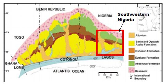
Figure 2: The Nigerian portion of Dahomey (Benin) Basin. After Ola-Buraimo, Oluwajana [31].

fig 3

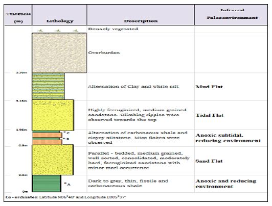
Figure 3: A Lithologic section of Arimogija – Okeluse exposure. After Ola-Buraimo, Oluwajana [31].

In the Nigerian sector of the basin the Cretaceous sequence, as compiled from outcrop and borehole records, consists of the Abeokuta Group, further divided into three geologic units: Ise, Afowo, and Araromi Formations. Ise Formation overlies the basement complex unconformably and comprises of coarse conglomeratic sediments [33,34]. Afowo Formation is composed of transitional to marine sands and sandstone with variable but thick interbedded shales and siltstone [35,36]. Araromi is the uppermost Formation and comprises shales and siltstone with interbeds of limestone and sands. The Tertiary sediments comprise Ewekoro, Akinbo, Oshosun, Ilaro, and Benin (bare coastal sand). The Ewekoro Formation comprises fossiliferous, well-bedded limestone while Akinbo and Oshosun Formations are made up of flaggy grey and black shales [37,38]. Glauconitic rock bands and phosphatic beds define the boundary between the Ewekoro and Akinbo Formations. The Ilaro and Benin Formations are predominantly coarse sandy estuarine, deltaic, and continental beds [31].

The Abeokuta Group

The sedimentary Formation of southwestern Nigeria, otherwise known as the Eastern Dahomey Basin, extending from the Nigeria/Benin border in the west of Makun-Omi and broken in the east. The Abeokuta Group is the oldest Formation, and it comprises of main sands with intercalations of argillaceous sediments, which lie unconformably on the crystalline basement complex formation [39,40]. This group can be subdivided into three geologic units;

  • The lse Formation, which overlies the basement complex and consists of pre-drift sediments of grits and siltstones and overlain by coarse-medium grained, loose sands interbedded generally by kaolinitic clays;
  • The Afowo Formation comprises intermediate to marine sands and sandstone with variable but thick interbedded shales and siltstones. The shale to sand ratio Increase upwards with the sediment becoming highly fossiliferous. The whole arrangement represents paralic sedimentation; and
  • The Araromi Formation, which is the youngest of the stratigraphic sequence, comprises shales and siltstones with Interbeds of limestone and sands. It Is opulently fossiliferous.

The Abeokuta Formation usually has a basal conglomerate with about 1 meter thick and mostly comprises poorly rounded quartz pebbles with a silicified and ferruginous sandstone matrix or a soft gritty white clay matrix [39]. The formation outcrops where there is no conglomerate, a coarse, poorly sorted pebbly sandstone with copious white clay establishes the basal bed. The superimposing sands are coarse-grained, clayey, micaceous, and ill-sorted, suggestive short distances of transportation, or short duration of weathering and possible derivation from the granitic rocks located to the northwards. Upward stratigraphically along with the outcrop areas, the shale content increases progressively in some places, particularly around Ijebu-Ode. Close to the embayment’s eastern margin, thin beds of lignite may be present together with a high impregnation of bitumen in the sand and clays. These features are displayed in most of the eastern part of the embayment, locally referred to as Tar sand. The basal beds’ upper horizons were found in some outcrops to contain thin beds of Oolitic ironstone. The stratigraphic dating from palynological studies indicates that the ages of the lower and upper limits of the neostratotype Formation are late Albian and late Senonian. This is a characteristic species for the late Turonian-early Senonian of the Ivory Coast and was reported from Gabon’s Coniacian-Campanian. Therefore, this pollen occurrence implies a late Senonian age for the Formation’s upper layers [39].

The Ise-Afowo, Araromi, Akinbo, and Ilaro Formations

Ise and Afowo Formations are similar; thus, the two geologic units are treated together in most literature [39,41,42]. The two formations contain sand and sandstones, but the latter is interbedded by thick of shale units. Similarly, the Ise, Afowo, and Abeokuta Formations showed a similar lithologic and electric log. The uppermost beds of Abeokuta Formation which outcrop in the Ijebu-Ode, Itori, Wasimi, and Ishaga, consist mainly of fine-coarse-grained sand which is occasionally interbedded by shale, mudstone, limestone, and silt. In most recent literature the Ise and Afowo Formations are discussed as Abeokuta Formation. The Abeokuta Formation consists mainly of grits, loose sand, sandstone, kaolinitic clay, and shale. It was further characterized as usually having a basal conglomerate or a basal ferruginised sandstone [39]. The Araromi Formation overlies the Afowo Formation and has been described as the youngest Cretaceous sediment in the eastern Dahomey Basin. It is composed of fine to medium-grained sandstone at the base, overlain by shales, siltstone with interbedded limestone, marl, and lignite. This Formation is highly fossiliferous [43]. The Ewekoro Formation overlies the Araromi Formation. It is an extensive limestone body, which is traceable over a distance of about 320 km from Ghana in the west, towards the eastern margin of the Dahomey (Benin) Basin in Nigeria [44,45]. It is Palaeocene in age. Superimposing the Ewekoro Formation is the Akinbo Formation, which is mainly composed of shale and clayey sequence. The clay stones are concretionary and are largely kaolinite. The Formation’s base is defined by the presence of a glauconitic band with lenses of limestones [43]. The Akinbo Formation and consists of greenish-grey or beige clay and shale with interbeds of sandstones. The shale is thickly laminated and glauconitic. The basal beds may consist of either, sandstones, mudstones, claystones, clay-shale, or shale. The Ilaro Formation superimposes the Oshosun Formation and consists of massive, yellowish poorly, consolidated, cross-bedded sandstones. The youngest stratigraphic sequence in this basin is the Benin Formation, otherwise known as the Coastal Plain Sands and contains poorly sorted sands with layers of clay units. The sands are occasionally interbedded and show transitional to continental characteristics. The age is from Oligocene to Recent [43]. Most of the boreholes constructed in the basin are either single-screened or multiple-screened and occasionally open wells are constructed through fractured basement rocks that produce a considerable amount of water. The Depth to water level hardly exceeds 24 meters. Most aquifers in this basin are found around 40 meters below the surface. These aquifers are rarely confined, and very few boreholes tap water below 60 meters [46]. The mean yield from boreholes is ~0.4 l/s. In the crystalline basement section of the basin, a borehole depth of 40–80 m is estimated. Data from available boreholes in the southern end of Kwara State extending to Osun State, indicate the range between 25–68 meters borehole depth. The overburden thickness is also highly variable, ranging between 3–24 meters. In places around Ibadan, the overburden thickness and borehole depth are within the same range. The thickness of the overburden aquifer in the rural areas of Oyo State is correlated to the tectonic fractures rather than weathering (regolith).

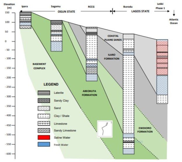
Borehole yield ranging from 1–2 l/s in the basement complex section is considered suitable for installing motorized submersible pumps. Borehole yields less than 0.5 l/s are also considered good for handpumps. The recharge into the weathered aquifer is predominantly through the infiltration of rainwater. Therefore, continued yields from motorized pumps may not be workable. Midwestern Nigeria’s coastal basin’s principal aquifers occur in sandy units and overburden/superficial deposits confined by shale and clay formations. The aquifers’ thickness is highly variable with first and third horizons reaching a thickness of about 200 meters and 250 meters at Lekki headland. The second horizon is roughly 100 meters thick (Figure 4). The estimated groundwater stored in the first aquifer horizon is about 2.87 × 10³ m3. The water table is mostly shallow, ranging 0.4–21 meters below the ground surface. It is estimated that annual fluctuation is less than 5 meters. The principal aquifer is within bare coastal sands, occasionally underlain by impermeable horizons of shale and clay units. Many high-yielding boreholes provide more than 30% of the water supply in Lagos and its hinterlands [46].

fig 4

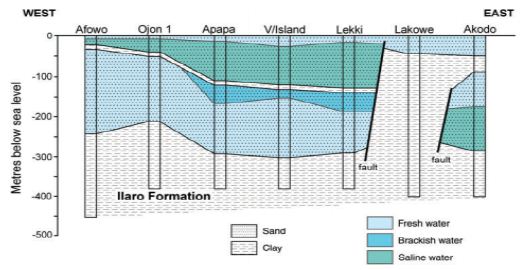
Figure 4: Typical hydrogeological section of coastal basins of southwestern Nigeria. After Adelana, Vrbka [46].

The geological succession in these basins simple, forming a simple monocline against the basement outcrop northward, with a slight faulting indication. The inclines are reportedly about 1° or less southwestwards (Table 1). The Basement Complex rocks superimpose more than 50% of the Coastal basins [47-49]. The Abeokuta Formation is the oldest outcropping sedimentary formation in the Ogun and Osse River Basin. This appeared to cover the basement complex directly. The Formation is in turn superimposed by the Ewekoro, Ilaro, and Benin Formations. The is the substantial development of alluvium in the coastal areas and along the course of the major drainage systems of the Rivers Ogun and Osse.

Table 1: Hydrogeology of coastal basins of southwestern Nigeria.
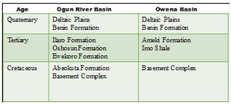
table 1

After Offodile [32]

The Abeokuta Formation

This is the oldest Formation in the Ogun Basin, outwardly covering the Basement Complex. The Formation thickness ranged from 250 to 300 meters, containing arkosic sandstones and grits, tending to be carbonaceous towards the bottom. There is an increase in thickness from about 250 meters in the western sections of the basin towards the Benin border. The basal conglomerates also were encountered. One of the outcrops gave the following units in Figure 5. The Abeokuta Formation has good potential for groundwater except that the bituminous constituents associated with the sands could affect groundwater quality. This Formation is being interrelated to the Nkporo Shale, east of the River Niger. The little report is existing about the groundwater potentials of the Abeokuta Formation. Nevertheless, its proximity to the Basement Complex and its high porosity, a substantial amount of groundwater is expected to be stored above the crystalline rock layer. This condition has been confirmed at the bottom near the Basement layer, intercepted by the borehole described in the following section. This Formation is outstanding in the basin. Hydrogeologically, groundwater in the basin’s northern parts is limited to the splintered and in-situ worn portions of the rocks. The in-situ worn portion either superimposes the unweathered basement or occurs within the unweathered basement [50].

fig 5

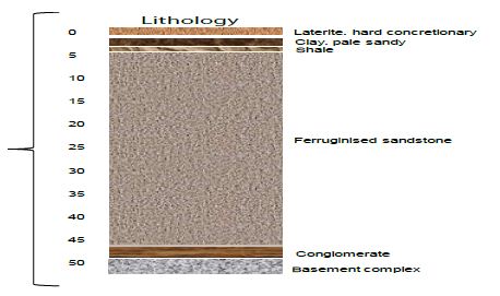
Figure 5: Section of Abeokuta Formation. After Offodile [32].

In the former, the worn materials create phreatic aquifers typically exploited through hand-dug shallow wells, while in the later, groundwater is confined in nature and can only be accessed through boreholes. Groundwater flow is strongly influenced by topography and two common types of springs, mainly, overland and slope springs have been observed in the area. Recharge to these aquifers is primarily by infiltrating rainfall and in some places, by the outflow from adjacent surface water. The recharge areas comprise decayed and splintered rocks in which pressure heads quickly spread through local water-bearing fractures and unified voids, thereby leading to an abrupt rise in ejections in response to rain. Spring discharges in the northern parts of the basin are very common in the rainy season but terminate totally during the dry season. The area underlain by sedimentary formations is regarded as having good groundwater potential due to an aquiferous sandy layer [50].

However, the success of boreholes in this basin is highly variable, and it could be credited to inferior drilling methods, or the frequent occurrence of the clayey matrix, which extends to seal the pores and reduce the absorptivity. The successful boreholes were reported from Aiyetoro and Ijebu Ode. Also, specific capacity ranging from 63 to 17550 list/hr/m (1300 gift) have been measured. Successful boreholes were also reported from Iboro, Imushin, and Ishaga as depicted below. In the eastern parts, within the Osse Basin, the Abeokuta Formation appears to thicken in Agenebode and Auchi’s higher regions, where the groundwater table is deep (120-300 meters). The low water table recorded is thought to be due to the aquifer’s high porosity, as typified in by the Kerri-Kerri Formation, in the Upper Benue Basin Nanka Sands of the Anambra Basin [32]. Some drilled boreholes in the Abeokuta Basin are shown in Figure 6. Figure 7 illustrates some successful boreholes in Abeokuta Formation. The GSN. BH. No. 2436 is located at Meko. The lies unconformably showed unconformity. It has a total depth of 57.9 meters. Although it penetrates the Basement Complex, yields are relatively low (1620 lits/hr (0.45 lits/sec)—the GSN. BH. No. 2612 was located at Igbogila. The borehole penetrates a Basement Complex section and has a total depth of 70.5 meters. Yield is relatively high (28350 lits/hr), or 7.87 lits/sec. it has a specific capacity of about 390.8 lits/hr—the GSN. BH. No. 2438 is located at Aiyetoro. The borehole penetrated a Basement Complex formation and showed unconformity. The total depth is about 55.9 meters. Yield is relatively low (2340 lit/hr), or 0.65 lits/sec (Offodile, 2002). Figure 7 further illustrates some boreholes penetrating the Abeokuta Formation. The GSN. BH. No. 2433 reached a depth of 48 meters below the ground level. This borehole’s actual location is unknown, but it is believed to penetrate the Abeokuta Formation. The borehole produced a yield of about 3600 lits/hr and had a specific capacity of 11880 lit/hr/m (Offodile, 2002). The GSN. BH. No. 2435 is located at Ishaga. It penetrated the basement complex (BC) and had a total depth of 75 meters. It had a yield of 31050 lits/hr. It also had a specific capacity of 3192.75 lit/hr/m [32]. The lithology is mainly sandy (Figure 7) – the GSN. BH. No. 2597 is located at Ijebu Ode about 46 km NE of the town. The borehole penetrated the BC and reached a depth of 54.6 meters. The yield obtained from this well is comparatively low (10800 lits/hr), with a specific capacity of 935.5 lits/hr/m. The last borehole in Figure 6 (GSN. BH. No. 1807), also lies unconformably on the BC. The well reached a depth of 72.8 meters and produced a yield of 13500 lits/hr, with a specific capacity of 4039.2 lit/hr/m [32]. Generally, boreholes penetrating the Abeokuta Formation has a higher proportion of sands.

fig 6

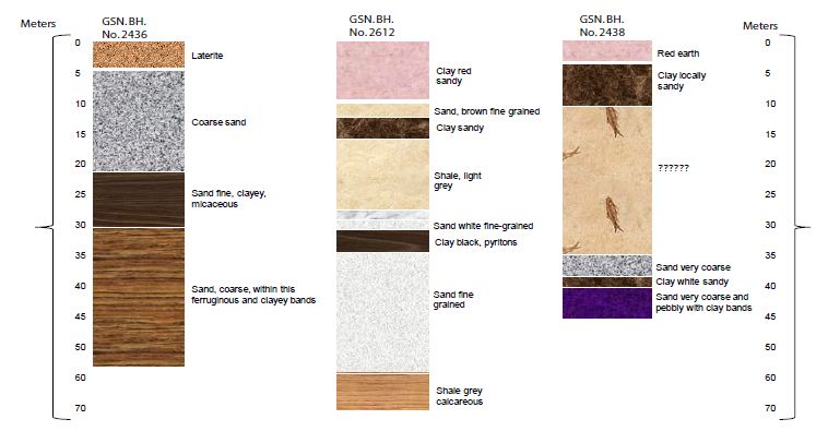
Figure 6: Lithological sections of boreholes in Abeokuta Formation. After Offodile [32].

fig 7

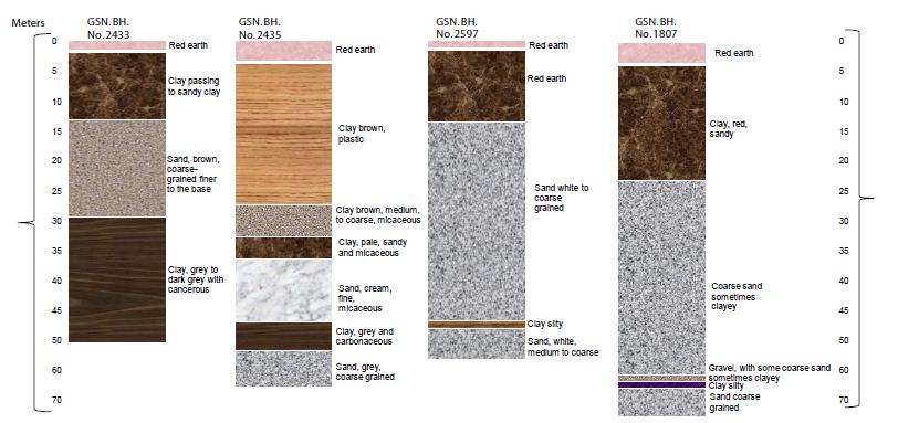
Figure 7: The lithology of boreholes in Abeokuta Formation. After Offodile [32].

The Ilaro Formation

The Ilaro Formation is comprised of fine to medium-grained which are reasonably well sorted. The Formation lies conformably on the Oshoshun Formation (Lower-Middle Eocene) and locally unconformably underneath the Benin Formation -Oligocene-Pleistocene [51-53]. The Ilaro Formation is typically Middle to Upper Eocene in age. The estimated thickness of this Formation is about 70 meters and displays rapid lateral facies changes. This can affect aquifer quality [54]. Hydrogeologically, not much information exists on the Ilaro Formation, though it is reported to be transitional to, and in part equivalent to the Ameki Formation. Given the Ilaro Formation’s geological physiognomies, its equivalent lateral part could be a good aquifer that can yield a substantial amount of water. However, GSN. BH. No. 2611 in Ilaro had reached a depth of 57 meters and gave a low yield of 2975 lits/hr and a specific capacity of 1023 lits/hr/m [32]. The lithology of this borehole is illustrated in Figure 8.

fig 8

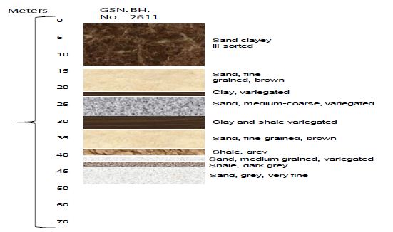
Figure 8: The lithology of the borehole in Ilaro. After Offodile [32].

The Benin Formation

The Benin Formation (Miocene-Recent) consists of thick bodies of ferruginous and white sands. The Formation lies conformably on Ilaro Formation. Friable, poorly sorted with intercalation of shale, clay, and sandy clay with lignite [55]. The Benin aquifer is an important reservoir of groundwater. It is well developed in the Osse Basin and underlies more than 50% of its sedimentary section. The Benin aquifer is underlain by the sandstones of and shales of the upper Ilaro Formation, consists of a sequence of predominant continental sands and some lenses of shales and clays proved to be up to 107.7 meters thick in the area. The cross-section of the Benin Basin is further illustrated below. The Benin Aquifer gives very high yields of up to 4500 lits/hr (10000 g/hr) in most parts of the outcrop area.

The water table is relatively shallow, ranging between 20 to 25 meters. The water quality is also good. By this Formation, the land area underlain extends from Ado-Odo, Ilaro, Ikeja, and Mushin, passing through Okitipupa of Ogun Basin, into a broad area Benin-Ugheli-Agbo province of Osse Basin, in Edo and Delta States [32]. The lithology of boreholes from the Benin formation is illustrated in Figure 8. The GSN. BH. No. 2608 is located at Ikeja, had a total depth of 99 meters. The yield from this borehole is comparatively high (55350 lits/hr) [32]. Figure 9 illustrates the lithology of Benin formation [56].

fig 9

Figure 9: Hydrogeologic Cross-section of the Benin Basin. After Oteri and Ayeni [56].

Figure 10 shows the specific capacity of this borehole is 9,220 lits/hr/m. This well penetrates the Benin Formation. The GSN. BH. No. 927 is located in Otta. The well had a depth of 243 meters. The remaining lithologies were not accessed. Yield from this borehole was estimated to be 22500 lits/hr in GSN. BH. No. 2599, located at Mushin penetrates a similar sequence, attained a depth of 108.6 meters. This well gave a yield of 32850 lits/hr (9 lits/sec). The specific capacity was 1930.5 lits/hr/m. This prolific yield is typical of the Benin Formation across the southwestern river basins of Nigeria. The Benin Formation is also very important in the Osse Owena Basin, where it is the primary groundwater source [32].

fig 10

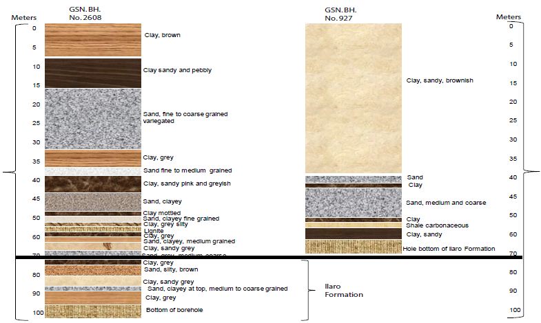
Figure 10: The lithology of the borehole in Ikeja and Otta. After Offodile [32].

The Deltaic Formation and Alluvial Deposits

This Formation contains alluvial deposits associated with Lagos’ coastal areas and the Osse Basin areas connecting to the Niger Delta Basin [57-59]. The hydrogeological conditions in areas were explained in studies on the Niger Delta Basin. Be sufficient to mention that the sandstone beds are limited in thickness and usually variable in the lateral extent. Furthermore, these aquifers have been exposed to saline water intrusion due to overdevelopment and seawater invasions. Correspondingly, the limitations in thickness and extent of the aquifers significantly reduce the boreholes’ specific capacity. The groundwater condition varies swiftly across the basins. In the Lagos region areas where the Formation appears to be least developed and has been polluted, the underlying Benin Formation provides a ready supply to the groundwater demand in the basin [32]. These comprise the Yewa, Ogun, and Oshun river networks’ vast basins, presenting a general alluvial development with considerable groundwater potential. The available drilling records have not distinguished this Formation. However, a 49275 lits/hr yield from GSN. BH. No. 2610 at Ibefun. The borehole was just 28.5 meters deep and had a specific capacity of 9234 lits/hr/m. This presents an excellent yield and underlines the high potential of these river basins’ alluvial deposits. The hydrogeology of these basins is similar to that of the Niger Delta Basin, discussed in the previous chapter.

Hydrogeological Condition in Coastal Basins of Southwestern Nigeria

The Ogun River Basin

The Ogun River Basin is one of the significant coastal basins located in southwestern Nigeria [60-62]. The basin is situated between latitudes 6° 26′ N and 9° 10’N and longitudes 2° 28’E and 4° 8 ‘E (Figure 11). About 98% of the basin area falls within Nigeria and the remaining 2% in the Benin Republic. The basin covers an of about 23,000 sqkm. The topography is generally low, with the gradient in the north-south direction. The Basin is drained by the Ogun River which had its source from the Iran hills at an elevation of about 530 meters above sea level. The river flows southwards over a distance of about 480 km before it discharges into the Lagos lagoon. The main tributaries of the Ogun River are the Ofiki and Opeki Rivers. Two seasons are distinguishable in the Ogun River Basin; a dry season from November to March and a wet season between April and October. The mean annual rainfall ranged from 900 mm in the northern parts to 2000 mm in the south. The total annual potential evapotranspiration ranged from 1600 and 1900 mm [63]. Hydrogeologically, very little is known about the Ogun Basin since the basin is often discussed in southwestern Nigeria’s coastal basins. However, Offodile [32], compiled data on borehole on borehole depths summarized in Table 2. There is not much reporting of hydrogeological physiognomies of the individual boreholes from western Nigeria’s coastal basins. Most of the boreholes in this basin penetrate the Pre Cambrian-Basement Complex. Yields from these boreholes are poorly known. However, GSN. BH. No. 2614 in Ewekoro gave an artesian flow of 90-135 lits/hr obtained near the borehole base. Similarly, GSN. BH. No. 1583 at Itori gave artesian flow at 81 meters. The estimated yield was 450 lits/hr and a specific capacity of 92.7 m 45000 lits/hr/m. Although, these two boreholes produced a substantial amount of water, a more detailed study on the hydrogeology Ogun Basin is required for further evaluation.

fig 11

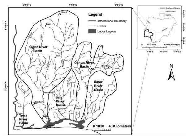
Figure 11: Ogun-Osun River Basins and the Adjacent Basins. After Oke, Martins [63].

Table 2: Borehole information from Ogun Basin.

S/no.

Borehole Locality (Abeokuta Formation)

GSN. BH. No. Total Depth (m) Depth to First Water (m) Final Depth to Water (m) Yield (lits/hr) Draw Down (m) Specific Capacity (lits/hr/m)

Remarks

1

Aiyetoro 2

2438 63 31.2 31.2 2340 15

Pre Cambrian-45.9-63 m

2

Aiyetoro 2

2439 53.7 20.7 20.7 18900 3.6 5250

Pre Cambrian-45.9-63 m

3

Ijebu Ife

1808 57 42 39.9 10655 10.6 1035
4

Ijebu Ode

2620

Abandoned Pre Cambrian-Very shallow

5

Ijebu Ode

2597 69.9 46.2 46.2 10800 11.4 945

Pre Cambrian-54.6-69.6 m

6

Ijebu Ode

2598 54

Abandoned Pre Cambrian-18.3-54 m

7

Imushin

1807 87 55.8 52.8 13500 3.3 4080

Pre Cambrian-72.9-87 m

8

Imushin

2616 75.9 51.9 35100 1.8 19500

Pre Cambrian-65.4-75 m

9

Ishage

2435 75 29.1 19.8 31050 9.6 3225

Pre Cambrian-67.8-75 m

10

Meko

2436 57.9 42.3 42.3 1620 10.5

Pre Cambrian-54.6-57.9 m

(a)                 Borehole Locality (Fugar Area)
11

Agenebodo

2604 127.2 105.9 105.9

Not tested

12

Fugar

1136 69.3

Abandoned

13

Fugar

1179 157.5 129.6 4500

14

Fugar

2603 157.8 129.6 129.6

Not tested

15

Ogbona

2613 213 183.3

Not tested

(b)                 Borehole Locality (Ewekoro Formation)
16

Ewekoro

2614 90 58500

Artesian flow 90-135 lits/hr Obtained near the bottom of the hole

17

Iboro2

2433 48 13.5 10.2 36000 3 1200

18

Labour

2434 33.6 32850 3 10950

19

Ifon2

2602 79.5 64.5 61.8 12600 2.1 6000

20

Igbogila2

2612 70.5 11.4 10.2 28350 11.7 2415

21

Itori

1583 96

Artesian flow at 81 m, 450 lits/hr; at 92.7 m 45000 lits

22

Yemoji

1590 348

(c)                 Borehole Locality (Ibeshe Area)
23

Ibeshe2

2437 121.2 57.5 57.9 10.26 9.3 1095

24

Ilaro

2611 132.9 17.4 20.4 26.55 22.5 1170

(d)                 Borehole Locality (Imo Shale)
25

Sabon Gida

2601 121.2 41.4 13.05 51 255

Artesian flow 900 to 1350 lits/hr

After Offodile [32]

The Osse Owena Basin

Also known as the Benin-Owena, River Basin occurs in Edo-State. The basin is situated within the Western Littoral Hydrological Area HA-6, one of the eight hydrological areas into which Nigeria is subdivided. The gauge station at which the hydrometric measurements were made is located at Osse River at Iguoriahki [64-66]. Hydrogeologically, this basin has not been well explored. Earlier, Offodile [32] summarised borehole information on this basin. Base on the borehole information presented in Table 3, it is clear that this basin has not been fully explored hydrogeologically.

Table 3: Borehole information from Osse Owena Basin.

Borehole Locality (Ameki Formation)

GSN. BH. No.

Total Depth (m) Depth to First Water (m) Final Depth to Water (m) Yield (lits/hr) Draw Down (m) Specific Capacity (lits/hr/m)

Remarks

1 Asaba

72

27.6 23.1 8325

2 Asaba

72

22.5 25.5 9450 3 31

3 Asaba

67.5

16.5 17.4 18000

4 Asaba

45.6

25.2 22.2 95850 3 31950

5 Asaba2

44.7

26.4 24 95850 4.2 22815

6 Isse-Uku

112.5

102.5

Abandoned

7 Isse-Uku

120

Abandoned

8 Iuue

241.5

Abandoned

9 Ogwashi-Uku

89.7

Abandoned

10 Uburu

114

108.5

Abandoned

Borehole Locality (Benin Formation)
11 Abafon

45.6

41.4 16.67

12 Ado Odo

96

I1 45000 2.7 9990

13 Ado Odo

14 Agbon

63

45 40500

15 Agbon

75 7.5 45000 4.5

16 Agbon

75 7.5 45000 32.13

17 Benin City

110.4 56.4 29.25 27.55

Borehole Locality (Ameki Formation)
18 Benin City

61.8 15 67500 2.1

19

Ethiope

34.5 10.5 49500 1.8

20 Sapele

37.5 4.8 31500

21 Sapele

37.5

No Data

22 Sapele

37.5 5.1 27000

23 Sapele

No Data

After Offodile [32]

The Osun River Basin

The Osun basin is drained by the Osun River system which rises from Oke-Mesi ridge, about 5 km North of Effon Alaiye along the Oshun and Ekiti States border and flows North through the Itawure gap to latitude 7° 53′ before winding its way westwards through Oshogbo and Ede and Southwards to enter Lagos lagoon about 8 km east of Epe [63,67]. A considerable part of the basin is underlain by rocks of the Precambrian Basement Complex, most of which are very ancient. This Basement Complex rocks showed significant variations in grain size and mineral composition [63]. The rocks are quartz gneisses and schist consisting essential of quartz with small amounts of white micaceous minerals. Even though the outcrops are visible, large areas are overlain by layers of laterite soil formed by weathering and decomposing the parent rock material. The minerals’ origin has been dealt with based on heavy mineral studies along the river basin. Moreover, the sedimentary rocks of Cretaceous and Tertiary deposits are found in the southern sector of the basin [63]. Generally, in coastal basins of southwestern Nigeria, groundwater is contained in four principal aquifers [56]:

  • The first is the shallow aquifer, which contained the Recent Sediments along the Atlantic Sea coast and river valleys. It is used for minimal private domestic supplies through dug wells and shallow boreholes.
  • The second and third aquifers are in the Coastal Plains Sands Formation. They are exploited through hand-dug shallow wells in some areas, shallow – and profound – boreholes. These aquifers provide considerable amounts of water for water supplies. This is the principal aquifer exploited, particularly in Lagos and its environs.
  • The fourth aquifer is the deep and highly productive Abeokuta formation, which was discussed in previous sections.

A few boreholes located mostly in Ikeja industrial area in Lagos only extract water from the fourth aquifer. The water from this aquifer is hot with temperatures as high as 80°C recorded in a few boreholes. This aquifer is undergoing massive development in adjoining Ogun State when encountered at shallower depths of between 300 and 550 meters. Figure 12 is a north-south geologic cross-section showing various Formations in the sedimentary basin. In Figure 12, a hydrogeologic cross-section from west to east along the coast shows both the lithologic and water-quality variations in the Coastal Plains Sands and Recent Sediments [56].

fig 12

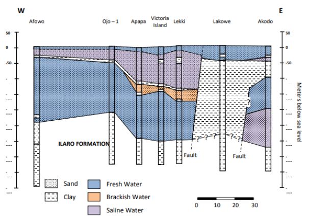
Figure 12: Hydrogeological cross-section of coastal basins along with Lagos State. After Oteri and Ayeni [56].

The delineation of shallow aquifers in the coastal plain sands of Okitipupa Area, Southwestern Nigeria, revealed two central aquifer units within the Okitipupa Area, Southwestern Nigeria [56]:

  • The upper/surficial aquifer system, which occurs at depths ranging from 5.8 m (around Agbabu) to 61.5 m (around Ikoya), and with materials of higher average resistivity (504.7 Ωm), suggestive of gravelly/coarse to medium-grained sand; and
  • The intermediate aquifer system, characterized by depth range of 32.1-127.5 m, average resistivity of 296.8 Ωm, typical of medium-grained sand saturated with water.

The highly resistive, impermeable materials overlying the aquifer units around Ajagba, Aiyesan, Agbetu, Ilutitun, Igbotako, and Erinj suggests that the aquifer units are less vulnerable to near-surface contaminants than in Agbabu, Igbisin, Ugbo, and Aboto where less resistive materials overlie aquifers. However, this indicates that the aquifer cannot be recharged in these areas. The geoelectric sequence suggests subsurface geology characterized by the alternation of sands/gravel, clay/shale, and sandstone occurring at varying depths with variable thicknesses. The sand and gravel layers constitute the aquifer units [56]. The aquifer units’ geoelectric parameters were determined by interpreting the sounding curves, assisted by the distinctive resistivity contrasts between the discrete geoelectric layers.

The upper and lower aquifer horizons work are referred to as the surficial (upper) and intermediate (lower) aquifers. In a different study by Adepelumi, Ako [68], which delineates saltwater intrusion into the freshwater aquifer of Lekki Peninsula, Lagos, Nigeria, the study delineates four distinct resistivity zones viz:

  • The unconsolidated dry sand having resistivity values ranging between 125 and 1,028 Xm represents the first layer;
  • The fresh water-saturated soil having resistivity values which correspond to 32–256 Xm is the second layer;
  • The third layer is interpreted as the mixing (transition) zone of fresh with brackish groundwater. The resistivity of this layer ranges from 4 to 32 Xm; and
  • Layer four is characterized by resistivities values generally below 4 Xm reflecting an aquifer possibly containing brine. The rock matrix, salinity, and water saturation are the major factors controlling the Formation’s resistivity. Furthermore, this study illustrates that saline water intrusion into the aquifers can be accurately mapped using the surface DC resistivity method.

The Crystalline Basement Terrain

The Basement Complex terrains of South-western Nigeria are underlain by Precambrian basement rocks, which comprise crystalline igneous and metamorphic rocks mostly granite/porphyritic granite, granite-gneiss, quartz-schist, migmatite as well as Augen-gneiss, Pegmatite intrusions and variably Migmatized Biotite-hornblende Gneiss [28,69,70]. Descriptions on the field and petrographic/mineralogical characteristics of the different rock types are subject to various works. Textural and compositional attributes are wide-ranging. Directional fabrics such as foliation, lineation, and lamination are often developed in the Gneisses, Schists, Quartzites, and Tectonized rocks [71]. From the hydrogeologic perspective, unweathered basement rock contains negligible groundwater; however, the significant aquiferous unit can develop within the weathered overburden and fractured bedrock. It is this weathered and fractured zone, which forms potential groundwater zones. However, several factors that usually contribute to the weathering and development of fracture systems in the basement rocks can be summarized as follows [71]: (i) Presence and stress components of fractures; as conduit zones, hydro-geomorphological conditions that dictate the influence of weathering agents; (ii) Hydro-climatic/temperature regimes that dictate chemical weathering pace; and (iii) Mineral contents of the rock which affect the degree of weathering/overburden thickness.

The availability of groundwater in Pre Cambrian-Basement of southwestern Nigeria depends not only on the geology but also on the complex interactions of the various hydroclimatic and geomorphologic factors [72,73]. Accordingly, several methods have been established to locate favourable sites for groundwater resources extraction within basement rocks. These include remote sensing geophysical methods and geomorphological studies [71]. Assessment of previous studies on groundwater in the crystalline basement terrain of southwestern Nigeria discovered that the hydrogeological setting of the terrain is characterized by weathered saprolite units with varied thickness over the different bedrock units, Porphyritic Granites, Granite-gneiss, Migmatite, Pegmatite, and Quartz-schist settings. Such a setting suggests the influence of rock types and mineralogy on the extent of fracturing and weathering. Consequently, groundwater occurrences in the study area are in localized, disconnected phreatic regolith aquifers, practically under unconfined to semi-confined conditions. Nonetheless, groundwater in the study area can be categorized under two central units: area with highly weathered and fractured bedrock units and poorly weathered/sparsely fractured bedrock units [71]. In an area with deeply weathered regolith and highly fractured zones, groundwater occurrences usually depend on the thickness of the water-bearing rock; this rock can be gravelly and fractured with possible quartz veins within the deep weathered zone of between 10 m to 30 m. These are characteristic of areas underlain in the study area by weathered crystalline and metamorphic rocks such as schist/quartz-schist, fractured granite-gneiss, and porphyritic granites as well as Augen gneiss with vertical fracture zones. These are generally characterized by moderate to high yield of about 75 m3/day and up to >150 m3/day. The borehole depth usually varies from 20 to 60 m, while the saturated thickness varies from 20 to 35 m below the ground surface [71]. In areas where the weathered zone is thin or absent, groundwater is usually tricky due to widely spaced fractures and the weathered zone’s localized zone/pockets. In the study area, these are characteristic of areas underlain by crystalline and metamorphic rocks, especially migmatite and variably Migmatized gneiss characterized by thin/shallow overburden unit of usually less than 10 meters in thickness and low yield of generally less than 75 m3/day. In such a setting also, the borehole depth varies from 20 to 30 m while saturated thickness varies from 8 to 20 m below the ground surface [71]. Nonetheless, towards the base of the weathered zone at the interface with the fresh bedrock, the permeability is usually high, allowing water to move freely due to the low proportion of clayey materials. However, deep-seated fractures are vital in such situations and can sometimes provide appreciable water supplies, mainly when tectonically controlled. Wells or boreholes that penetrate this horizon can usually provide sufficient water to sustain even hand-dug wells. Due to the complex interactions of the various factors affecting weathering in a typical basement complex setting like the study area, the groundwater potential zone distribution can be erratic and may not be present in some locations [71]. The analysis that involved characterization of weathered overburden revealed estimated overburden thickness using geoelectrical VES surveys from 3.8 to 50 meters with a mean value of about 20 meters as dictated by bedrock types. These values are within the range of values obtained for similar Basement Complex terrains of Africa. Furthermore, it was observed that areas with thin/shallow overburden coincided mostly with areas underlain by variably Migmatized gneiss complex, while the area with thicker overburden unit coincided with area mainly underlain by schist. However, the quartzite/quartz-schist setting coincided with areas of moderate to shallow overburden thickness [71]. In a nutshell, the varied thickness and the weathered overburden units’ isolated pockets also confirm the localized nature of weathered basement aquifers under the crystalline basement setting. The implication of this lies in the fact that there is the need for careful characterization and delineation of areas of possible fracturing and deep weathering as an aquiferous zone in respect of groundwater developments in Basement Complex settings of the study area. Therefore, the present study addresses the aspect of characterization of the groundwater potential using integrated GIS, RS, and MCDA techniques in conjunction with conventional hydrological and hydrogeological data [71]. Although the hydrogeology of southwestern Nigeria’s coastal basins is well described in the literature, a comprehensive description of its hydrochemistry has been lacking. The following section presents a synthesis of physicochemical physiognomies of groundwater in the basin.

Groundwater Chemistry

Physical Chemistry

Figures 13-15 present a summary of groundwater’s physical and chemical parameters in southwestern Nigeria’s coastal basins. Evaluation of pH concentration from 210 locations showed that pH ranged from 3.9 to 10.2 with a mean pH value of 7.4. Generally drinking water having pH < 7 is measured as acidic, and pH > 7 is considered basic. The normal range for pH in surface water systems is 6.5 to 8.5 and for groundwater aquifers 6 to 8.5 [74-76]. Unlike the Niger Delta Basin, groundwater in coastal basins of southwestern Nigeria is slightly alkaline. Alkalinity is a degree of the water’s capacity to resists a change in pH that would tend to make the water more acidic. The measurement of alkalinity and pH is needed to determine the water’s corrosivity [77-80]. The pH of clean water is 7 at 25°C, but when exposed to the atmosphere’s carbon dioxide, this equilibrium results in a pH of approximately 5.2. Because of the association of pH with atmospheric gasses and temperature, it is strongly recommended that the water is tested as soon as possible. The water’s pH is not a measure of the acidic or basic solution’s strength and alone does not provide a full picture of the characteristics or limitations with the water supply. In general, groundwater sources with low pH (< 6.5) could be acidic, soft, and corrosive. Therefore, the water could leach metal ions such as iron, manganese, copper, lead, zinc from the aquifer, plumbing fixtures, and piping. Consequently, groundwater with low pH could contain elevated levels of toxic metals, cause premature damage to metal piping, and have associated aesthetic problems such as a metallic or sour taste, laundry staining, and the characteristic blue-green staining of sinks and drains [81-83].

Groundwater sources having pH > 8.5 could indicate that the water is hard [84-86]. Hard water does not pose a health risk but can cause aesthetic problems. These problems include:

  • Formation of a ‘scale’ or precipitate on piping and fixtures causing water pressures and the interior diameter of piping to decrease;
  • Causes an alkali taste to the water and can make coffee taste bitter;
  • Formation of a scale or deposit on dishes, utensils, and laundry basins;
  • Difficulty in getting soaps and detergents to foam and Formation of insoluble precipitates on clothing, etc.; and Decreases efficiency of electric water heaters.

The temperature ranged from 22.7 to 30.5°C, with a mean value of 27.5°C. The causes for the temperature rise in aquifers are numerous, and these are directly linked to the continuing structural developments and the existing uses at the earth’s surface. These influences can be direct or indirect. The direct influences on the groundwater temperature include all heat inputs to the groundwater through the sewage network, district-heat pipes, power lines, and sources connected with groundwater heat use and storage [87-89]. The indirect influences on groundwater temperature processes are linked with urbanization-related changes in the heat balance in the near-surface atmosphere. The most important factors are:

  • The disturbance of the water balance due to a high degree of surface imperviousness;
  • The change of soil characteristics caused by an aggregation of structures (differences in the near-surface heat input and heat capacity);
  • Changes in the irradiance balance by changes in the atmospheric composition; and
  • Anthropogenic heat generation (domestic heating, industry, and transport).

The differences mentioned above cause changes in the heat balance by comparison with the areas surrounding the city. The city heats itself slowly, stores more heat overall, and passes it on again slowly to the surrounding areas, i.e., it can generally be considered an enormous heat storage unit [90,91]. Over the long term, this process increases the annual mean air and soil temperatures. The long-term warming of the near-surface soil also leads to a heating of the groundwater. Since the temperature affects the physical qualities and the groundwater’s chemical and biological nature, deterioration of groundwater quality and an impairment of the groundwater fauna may result from high temperatures [92-94]. The concentration of EC was synthesized from 177 locations from the basins. Conductivity values ranged from 31.9 to 1643 µS/cm with a mean value of 526.47 µS/cm. Electrical conductivity is widely used for monitoring the mixing of fresh and saline water, for separating stream hydrographs, and for geophysical mapping of contaminated groundwater [95,96]. Distilled water should typically have an EC of less than 0.3 µS/cm. For groundwater, EC values greater than 500 µS cm-1 indicate that the water may be polluted, although values as high as 2000 µS/cm may be acceptable for irrigation water [97,98]. In Europe, the EC of drinking water should be no more than 2500 µS/cm; water with a higher TDS may have water quality problems and be unpleasant to drink [99-101]. Synthesis of hardness from 211 locations revealed that hardness ranged from 11 to 3215 mg/l with a mean value of 467.05 mg/l. Initially, water hardness was understood to be the capacity of water to precipitate soap. Hard water does not allow soap to form as many suds. Water high in hardness is detrimental to plumbing and will reduce the life of water heaters. Water softeners will typically reduce hardness to below 10 mg/l. However, they replace the calcium and magnesium metals with sodium which is undesirable for low salt intake diets [102-104]. Water softener companies often discuss hardness in ‘Grains per Gallon’ instead of the standard units mg/l. To convert hardness from mg/L to grains per gallon, multiply mg/l by 17. Thus, 525 mg/l is equal to 31 gram/gallon. Salinity ranged from 0.08 to 1109 mg/l with a mean value of 178.90 mg/l. There is a substantial reporting on salinity in coastal basins of southwestern Nigeria. All-natural water holds some salt level, and in groundwater, the concentration can naturally vary from fresh to saltier-than-seawater. While small amounts of salt are vital for life, high levels can limit groundwater use and affect ecosystems that depend on groundwater. Small quantities of salt are deposited on the landscape every time it rains. Evaporation and plant transpiration remove water from the landscape but leave the salt behind. It concentrates salt over time. Evaporation can also directly increase groundwater salinity in areas where groundwater is close to the surface. Old groundwater can also become saltier as it passes through aquifers and picks up salts from dissolved minerals.

Although salt in the southwestern Nigeria landscape’s coastal aquifers is natural, groundwater and salt movement’s salinity into groundwater-dependent ecosystems can be increased by human activities. Increases in groundwater salinity can be caused by:

  • Increased groundwater recharge because of irrigation, which mobilizes salts naturally accumulated in the soil (irrigation salinity);
  • Increased groundwater recharge because of land clearing, bringing groundwater near the land surface, causing evaporation from the soil surface and salt accumulation (dryland salinity);
  • Leaking pipes, over-watering of gardens, and runoff from compacted surfaces can raise groundwater levels and concentrate salts in urban areas, which can lead to salt damage on buildings and roads (urban salinity);
  • Over-pumping near the coast, which can cause seawater to seep into replenishing water levels.

Groundwater salinity can also be reduced at times, such as when rapid recharge from flooding flushes out or dilutes salty groundwater. Broadscale changes in groundwater salinity occur very slowly, over decades or longer. Therefore, groundwater salinity is usually monitored rarely except where human impacts are of concern. Measurements on Turbidity, TSS, and Alkalinity were not much in the coastal basins of southwestern Nigeria. Turbidity ranged from 0.86 to 26.34 mg/l, with a mean value of 8.06 mg/l. This estimate was based on two studies (Figure 13f). Therefore, more reporting on turbidity is required in the basin. There is currently little information regarding turbidity in groundwater, and the cause is not fully understood. The common assumption is that groundwater turbidity indicates a fast transport pathway connecting potentially contaminated surface water with the aquifer. Studies found no relationship between turbidity and microbiology, although Chalk sources appear more susceptible to E. coli than other aquifers [105]. The occurrence of turbidity tends to be site-specific with a variety of causes. Mitigation measures in groundwater might include variable speed pumps, automatic pumping to waste, blending, or engineered solutions. Discussion on TSS was based on one study (Figure 13g). Total suspended solids ranged from 153 to 1109 mg/l with a mean value of 472.67 mg/l. Total Suspended Solids (TSS), also known as non-filterable residue, are those solids (minerals and organic material) that remain trapped on a 1.2 µm filter. Suspended solids can enter groundwater through runoff from industrial, urban, or agricultural areas [106]. Elevated TSS can reduce water clarity, degrade habitats, clog fish gills, decrease photosynthetic activity, and cause an increase in water temperature. TSS has no drinking water standard; drinking water with high TSS concentration can increase people’s severity with liver diseases. Similarly, there is not much reporting on alkalinity from these basins. Alkalinity ranged from 0.3 to 1.5 mg/l, with a mean concentration of 0.67 mg/l (Figure 13h). Alkalinity is not a chemical in water, but, instead, it is a property of water-dependent on the presence of certain chemicals in the water, such as bicarbonates, carbonates, and hydroxides. Groundwater aquifers with high alkalinity will experience less of a change in its acidity, such as acidic water, such as acid rain or an acid spill, introduced into the water body [107-109]. In a surface water body, such as a lake, the water’s alkalinity comes mostly from the lake’s rocks and land. Precipitation falls in the lake’s watershed, and most of the water entering the lake comes from runoff over the landscape. If the landscape is in an area containing rocks such as limestone, then the runoff picks up chemicals such as calcium carbonate (CaCO3), which raises the water’s pH and alkalinity. In areas where the geology contains large amounts of granite, lakes will have lower alkalinity. A pond in a suburban area, even in a granite-heavy area, as in some parts on the coastal basins (e.g., Lagos and its environs), could have high alkalinity due to runoff from home lawns where limestone has been applied. However, studies are required for further evaluation. Studies on dissolved oxygen from coastal basins of southwestern Nigeria are quite small in number. Ayolabi, Folorunso [110]’s integrated geophysical and geochemical methods for environmental assessment of the municipal dumpsite system in Lagos revealed DO ranging between 4 to 4.4 mg/l with a mean value of 4.1 mg/l. Similarly, Awomeso, Taiwo [111]’s study on the pollution of a waterbody by textile industry effluents in Lagos, Nigeria showed that COD concentration varies with distance from the discharge point. The concentration of was 890 mg/l at 0 meters, 600 mg/l at 50 meters, 214 mg/l at 100 meters, 1703 at 150 meters, 1172 ta 200 meters, 10 mg/l at 250 meters, 1693 mg/l at 300 meters, 860 mg/l at 350 meters, 1901 mg/l at 400 meters and 10 mg/l at 450 meters respectively. Omale and Longe [112]’s, assessment of the impact of abattoir effluents on River Illo, Ota, Nigeria showed that BOD ranged from 140 to 670 mg/l with a mean value of 333.33 mg/l. Most of the studies reporting BOD came from surface water bodies. Groundwater is yet to be fully explored in southwestern Nigeria’s coastal basins, based on these parameters. Dissolved oxygen significantly affects groundwater quality by regulating the valence state of trace metals and constraining dissolved organic species’ bacterial metabolism [113-115]. Consequently, the measurement of dissolved oxygen concentration should be considered vital in most water quality researches. Measurements of dissolved oxygen have been often ignored in groundwater monitoring. Oxygen has regularly been assumed absent below the water table; O2 measurements are not mandated by drinking water standards. Regular organic debris and organic waste derived from wastewater treatment plants, failing septic systems, and agricultural and urban runoff act as food sources for water-borne bacteria. Bacteria decompose these organic constituents using DO, consequently reducing the DO present for aquatic organisms. Chemical oxygen demand does not discriminate between biologically available and inert organic matter, and it is a measure of the total quantity of oxygen required to oxidize all organic material into carbon dioxide and water [116-119]. The COD values are always greater than BOD values, but COD measurements can be made in a few hours while BOD measurements take five days. Since parameters play a significant role in groundwater quality, it is recommended that such parameters are measured throughout the coastal basin of southwestern Nigeria. Figure 14 presents the groundwater classification based on pH, Hardness, Conductivity, and TDS. Based on pH 50.95% of groundwater sources in coastal basins of southwestern Nigeria fall in neutral class, 35.24% fall in acidic class, and 13.80% fall in alkaline class. Conversely, total hardness is also varying in the basin. About 43.37% of groundwater sources fall in soft class, 24.29% fall in intermediate class, 23.72% fall in hard class, and 9.60% fall in the very hard-water class. About 67.80% of groundwater sources have conductivity below 750 µS/cm, and 32.24% have EC values between 750 to 2250 µS/cm. Low TDS levels further show the low conductivity of groundwater sources in the basin. About 62.55% groundwater sources have TDS below 500 mg/l, 27.96% have TDS concentration between 500 to 1000 mg/l, 9.00% have TDS level between 1000 to 3000 mg/l and 0.47% have TDS above 3000 mg/l. This variability is further illustrated in Figure 14d.

fig 13

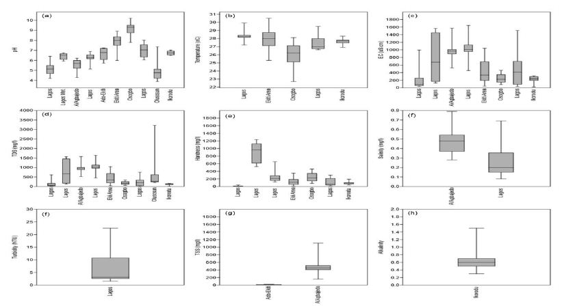
Figure 13: Hydrogeological cross-section of coastal basins along with Lagos State.

fig 14

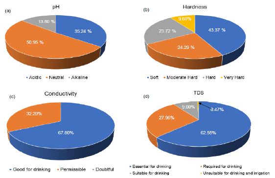
Figure 14: Groundwater classification (a) pH, (b) Total hardness, (c) Conductivity and (d) TDS.

Cation Chemistry

Understanding the chemical physiognomies of groundwater is essential as a result of their contrasting sources. As soon as their concentration is above the suggested reference guidelines, these prerequisites may render groundwater unusable. Chemical essentials including Ca, Mg, Cu, Cd, B, Al, K, PO4, SO4 As, and Cl, for instance, are primarily derived from rocks. Nonetheless, elements like NO3 and SO4 are derived mainly from anthropogenic sources [118,119]. Understanding the derivation and absorption level of these chemical elements in groundwater is needed for effective groundwater management. Generally, there is little reporting on Al, NH4, and southwestern Nigeria’s coastal basins. For instance, Ayolabi, Folorunso [110]’s analysis of the municipal dumpsite system in Lagos showed Al ranged from 0.001 to 1.641 mg/l with a mean value of 0.29 mg/l.

Longe and Enekwechi [120] investigated potential groundwater impacts, and the influence of local hydrogeology on natural attenuation of leachate at a municipal landfill from Olusosun landfill showed that NH4 ranged from 0.14 to 1.5 mg/l with an average value of 0.41 mg/l. A review of the level of arsenic in potable water sources in Nigeria and their potential health impacts by Izah and Srivastav [121]’s analysis showed that arsenic concentration in western Nigeria ranged from 0.00 to 0.38 mg/l at Ibadan, 0.00 to 0.05 mg/l in Odeda region, 0.03 to 0.47 mg/l at Ijebu land and 0.01 to 0.70 mg/l at Igun-ijesha. People are exposed to elevated levels of inorganic arsenic through drinking contaminated water, using contaminated water in food preparation and irrigation of food crops, industrial processes, eating contaminated food and smoking tobacco. Long-term exposure to inorganic arsenic, mainly through drinking water and food, can lead to chronic arsenic poisoning. Skin lesions and skin cancer are the most characteristic effects. The SON has recommended 0.2 mg/l as a maximum permissible limit in drinking water. Aluminium is an excellent metal in the earth’s crust and is regularly found in the form of silicates such as feldspar. The oxide of Al known as bauxite provides a suitable source of uncontaminated ore. Aluminium can be selectively leached from rock and soil to enter groundwater aquifer. Aluminium is known to exist in groundwater in concentrations ranging from 0.1 ppm to 8.0 ppm. Al can be present as Aluminum Hydroxide, a residual from the municipal feeding of aluminium (Aluminum Sulfate), or as Sodium Aluminate from clarification or precipitation softening. It has been known to cause deposits in cooling systems and contributes to the boiler scale. Aluminium may precipitate at normal drinking water pH levels and accumulate as a white gelatinous deposit. Aluminium is controlled in drinking water with a recommended Secondary Maximum Contaminant Level (SMCL). SMCL’s are used when the taste, odour, or appearance of water may be adversely affected. In this case, the WHO [122] established that an Al concentration above 0.1–0.2 mg/l might impact colour but recognize that level may not be appropriate for all water supplies. The Nigerian Standard for Drinking Water Quality (NSDWQ) has recommended 0.2 mg/l as a maximum permissible limit because of potential neuro-degenerative disorders associated with high Al concentrations in water. The natural levels of NH4 in groundwater and surface water are usually below 0.2 mg/litre. Anaerobic groundwaters may contain up to 3 mg/l. Leached effluents from the concentrated rearing of farm animals can give rise to much higher levels in groundwater. Ammonia pollution can also rise from cement mortar pipe linings. Ammonia is an indicator of possible bacterial, sewage, and animal waste effluence. Contact from environmental sources is insignificant in comparison with the endogenous synthesis of NH4. Toxicological effects are observed only at exposures above about 200 mg/kg of body weight. Ammonia in drinking water is not of immediate health significance, and consequently, no health-based guideline value is proposed by SON. There are few studies on Barium concentration in groundwater from coastal basins of southwestern Nigeria. Odukoya and Abimbola [123]’s assessment of contamination of surface and groundwater within and around two dumpsites in Lagos revealed that Ba concentrations ranged from 40 to 100 mg/l with a mean value of 49 mg/l within and around abandoned dumpsite. Barium also ranged from <0.001 to 80 mg/l with a mean value of 56 mg/l within and around active dumpsite. Barium is available as a trace element in both igneous and sedimentary rocks. Even though it is not found free, it occurs in several compounds, most commonly barium sulfate (or barite) and, to a lesser extent, barium carbonate (or witherite). Barium goes into the environment naturally via the weathering of rocks and minerals. Anthropogenic releases are primarily connected with industrial processes. The over-all population is exposed to Ba through the ingestion of drinking water and foods, usually at low levels. Figure 15a presents a synthesis of Ca from groundwater from coastal basins of southwestern Nigeria. Calcium ranged from 1.49 to 1460 mg/l with a mean value of 56.78 mg/l. Calcium in drinking water is beneficial, but it is important to note that calcium is a significant constituent of hardness. Based on SON guidelines, Ca is not limited to drinking water. Based on the results of the WHO meeting of experts held in Rome, Italy, in 2003 to discuss nutrients in drinking water [124], the assembly focused its attention on Ca and Mg, for which, next to F, a sign of health benefits accompanied by their existence in drinking water is robust. The Ca’s insufficient consumption has been accompanied by increased risks of osteoporosis, nephrolithiasis (kidney stones), colorectal cancer, hypertension and stroke, coronary artery disease, insulin resistance, and obesity. Most of these disorders have treatments but no cures. Due to a lack of convincing evidence for Ca’s role as a single influential element about these diseases, estimates of the Ca requirement have been made based on bone health outcomes to improve bone mineral density. Calcium is exclusive among nutrients because the body’s reserve is also functional: increasing bone mass is correlated to a decrease in fracture risk. There relatively high Ca level in these basins could be beneficial to the health of the people living there. Figure 15b presents a synthesis of Mg from groundwater in coastal basins of southwestern Nigeria. Evaluation of Mg from 183 sites across these basins showed that Ca ranged from 0 to 108 mg/l with a mean value of 12.26 mg/l. Based on the NSDWQ [125] reference guidelines, 0.2 mg/l was suggested as the maximum permissible Mg concentration in drinking water. The relatively high Ca and Mg recorded in these basins have resulted in the hard water as 56.63% of groundwater in these basins is either moderately hard, hard, or very hard. Numerous epidemiologic researches carried out during recent years have established an inverse relationship between water hardness and death from cardiovascular disease. Many recommendations leave been offered concerning, the causal agent for the association between death from cardiovascular disease and water hardness. Two standards have been debated: a toxic effect brought by the contamination of lead or cadmium or a shielding effect from Ca or Mg’s water content. What is vital is to limit the concentrations of these elements in drinking water. Figure 15c presents a synthesis of Mn from groundwater across the coastal basins of southwestern Nigeria. Manganese ranged from <0.001 to 108 mg/l with a mean concentration of 10.05 mg/l. The SON has recommended 0.2 mg/l Mn as the maximum permissible limit in drinking water due to the neurological disorder associated with water ingestions having a high Mn level [125]. Manganese has recently come under inspection in drinking water due to its possible toxicity and its impairment to water distribution networks. Manganese is rarely found alone in groundwater. It is often found in iron-bearing waters but is rarer than iron. Chemically it can be measured as a close relative of iron since it occurs in much the same iron forms. When manganese is available in groundwater, it is as annoying as iron, perhaps even more. At low concentrations, it produces incredibly objectionable stains on everything with which it comes in contact. Evaluation of K from 207 sites (Figure 15d), in the coastal basin of southwestern Nigeria, showed that K ranged from <0.001 to 341.7 mg/l with a mean value of 24.77 mg/l. Potassium is an essential electrolyte, which is a mineral required by the body to function correctly. Potassium is especially vital for nerves and muscles, including the heart. While K is central to human health, too much ingestion of K can be just as harmful as, or worse than, not getting enough. Usually, kidneys keep a healthy balance of K by flushing excess potassium out of the body. However, for many reasons, the level of potassium in the blood can be too high. This is called Hyperkalemia, or high potassium. The NSDWQ [125], issued no guidelines on K levels in drinking water. Figure 15e presents a synthesis of Na from groundwater across the coastal basins of southwestern Nigeria. Sodium concentration from 152 sites showed that Na ranged from <90.001 to 483.42 mg/l with a mean value of 38.02 mg/l. There is an increasing call to use K in combination with Na to treat and soften drinking water. However, this would cause the level of K in drinking water to increase. The WHO found that the level of K found in drinking water would present no health concerns for healthy adults; though, for specific populations with comprised renal functions, such as infants or individuals suffering from specific diseases, there is the likelihood of adverse health effects. Sodium is not measured to be toxic. The human body requires Na to maintain blood pressure, control fluid levels, and normal nerve and muscle function. However, there are no health-based criteria for Na in drinking water. Only a small amount of the Na we ingest practically comes from water. As a substitute, the standard for Na is based on taste. The mean Na concentration in these basins is below [125] recommended value (200 mg/l).

Quality assessment of groundwater in the vicinity of dumpsites in Ifo and Lagos, Southwestern Nigeria by Majolagbe, Kasali [126], showed that Cd concentration was below the detection limit at Ifo, whereas, mean Cd concentration was 0.005 in Lagos. In the same vein, groundwater quality assessment in a typical rural settlement (Igbora, Oyo state,) in southwest Nigeria by Adekunle, Adetunji [127], showed Cd concentration varies with distance from dumpsites. The Mean Cd concentration was 0.78 mg/l at 50 meters, 0.30 mg/l at 100 meters, 0.32 mg/l at 150 meters, and 0.30 mg/l at 200 meters away from during the dry season. Cadmium concentration was 0.34 mg/l at 50 meters, 0.32 mg/l at 100 meters, 0.30 mg/l at 150 mg/l and 0.24 mg/l at 200 meters away from dumpsite during wet season. Ayolabi, Folorunso [110]’s assessment of the municipal dumpsite system in Lagos indicated that Cd ranged from <0.001 to 0.025 mg/l. There are many studies on Cd in these basins, but the underline reasons for higher Cd in groundwater need to be understood. Many studies have been carried out to decode relationships between geological environment, potable/drinking water, and diseases as they were considered to have caused suffering due to diseases among people. Chronic anaemia can be caused by protracted exposure to drink water polluted with Cd. The Cd’s accumulation is established in the kidney under such conditions, resulting in cancer and cardiovascular diseases. The NSDWQ [125] has limit Cd concentration in drinking water to be 0.003 mg/l. Cadmium is restrained in drinking water because of its toxic effects on the kidney. Assessment of groundwater fluoride and dental fluorosis in Southwestern Nigeria by Gbadebo [128], revealed that groundwater samples from Abeokuta Metropolis (i.e., basement complex terrain) had F concentrations in the range of 0.65 to 1.20 mg/l. These values were lower than the F contents in the groundwater samples from Ewekoro peri-urban and Lagos metropolis where the values ranged between 1.10 to 1.45 and 0.15 and 2.20 mg/l, respectively. The F concentrations in nearly all locations were generally above the WHO recommended 0.6 mg/l. The study also revealed that the F distribution of groundwater samples from the different geological terrain was more dependent on pH and TDS than on temperature. The result of the analyzed social-demographic characteristics of the residents indicated that the adults (between the age of 20 and >40 years) showed dental decay than the adolescent (<20 years). This indicates an incidence of dental fluorosis by the high fluoride content in the populace’s drinking water. Conversely, evaluation of groundwater contamination in Ibadan, South-West Nigeria by Egbinola and Amanambu [129], revealed that F concentration is above the recommended limits in 13% and 100% the dry and wet season samples. The occurrence of F in groundwater has become one of the most significant toxicological environmental hazards worldwide. Fluoride in groundwater is due to the weathering and leaching of fluoride-bearing minerals from rocks and sediments. When consumed in small quantities (<0.5 mg/l), F is advantageous in promoting dental health by reducing dental caries, but higher concentrations (>1.5 mg/l) may cause fluorosis [130]. It is projected that about 200 million people, from among 25 nations the world over, may suffer from fluorosis and the causes have been attributed to fluoride pollution in groundwater including Nigeria. High F concentration in groundwater is expected from sodium bicarbonate-type water, which is calcium deficient. The alkalinity of water also mobilises fluoride from fluorite (CaF2) [131-133]. Exposure to F in humans is related to:

i. Fluoride concentration in drinking water

ii. Duration of consumption; and

iii. The climate of the area. In hotter climates where water consumption is more significant, exposure doses of fluoride (F) need to be modified based on mean F intake.

Many cost-effective and straightforward measures for water defluoridation methods are already known. Nonetheless, the benefits of such methods have not reached the affected rural population due to limitations. Consequently, there is a need to develop workable plans to provide fluoride-safe drinking water to rural communities [130]. There are few studies reporting lead in groundwater from coastal basins of southwestern Nigeria. An assessment of drinking water quality using the Water Quality Index in Ado-Ekiti and environs, by Olowe, Oluyege [134], showed that Pb ranged from <0.001-7.0 mg/l with a mean value of 1.94 mg/l. The quality assessment of groundwater in the vicinity of dumpsites in Ifo and Lagos, Southwestern Nigeria by Majolagbe, Kasali [126], showed that Pb concentrations at Ifo were below the detection limit. The Pb level at Lagos was 0.003 mg/l, and this value is below NSDWQ [125], reference guidelines. The primary reason for restraining Pb in groundwater is that Pb is associated with cancer, interfering with Vitamin D metabolism, affects mental development in infants, and is toxic to central and peripheral nervous systems.

Studies on Mercury are few in coastal basins of southwestern Nigeria. The geostatistical exploration of the dataset assessing the heavy metal contamination in Ewekoro limestone, Southwestern Nigeria by Oyeyemi, Aizebeokhai [135], showed that Hg ranged from 0.002 to 0.38 mg/kg with an average value of 0.12 mg/kg. The absence of Hg reporting groundwater in these basins at the time of this study revealed a possible research gap in groundwater quality in southwestern Nigeria’s coastal basins. Mercury is a scarce element in the Earth’s crust, having an average crustal abundance by mass of only 0.08 parts per million (ppm). Typical Hg sources comprise volcanoes, geologic deposits of Hg, volatilization from the ocean, and some geothermal springs. Nearly half of all Hg released to the environment is natural in origin. About 5,000 tons of Hg is released to the environment per year due to anthropogenic activities worldwide. The NSDWQ [125] has recommended 0.001 mg/l of Hg as the maximum permissible limit for Hg in drinking water due to its health effects on the kidney and central nervous system [125].

Figure 15f presents a synthesis of Ni from groundwater in coastal basins of southwestern Nigeria. Ni ranged from <0.001 to 9.2 mg/l with a mean concentration value of 1.84 mg/l. The NSDWQ [125], set 0.02 mg/l as the maximum permissible limit of Ni in drinking water, because of possible carcinogenicity. The risk of developing cancer from the ingestion of Ni contaminated water is high in western Nigeria since the average Ni (1.84 mg/l) is very much higher than the NSDWQ [125] reference guidelines. Nickel absorptions in groundwater hang on the soil use, pH, and depth of sampling. The mean concentration in groundwater in the coastal basins of western Nigeria is 1.84 mg/l. This value is very much high. Acid rain raises the mobility of Ni in the soil and thus might increase Ni concentrations in groundwater. In groundwater with a pH below 6.2, Ni concentrations up to 0.098 mg/l have been measured. The acidic composition of groundwater sources (35.24%) perhaps is responsible for high Ni levels in the basins. Table 4 shows silica concentrations in groundwater from Abeokuta. Silica varied markedly between the studied locations. The range was higher at Ikereku 12.5-16.4 mg/l [136]. Silica in groundwater has become an exciting element to hydrogeologists as an index to aquifers’ general lithology. Groundwater travelling slowly in the subsurface will approach chemical equilibrium with minerals present in the aquifers. Under average temperature and pressure, mean silica concentrations in groundwater vary from low values of about 7 mg/l in carbonate aquifers to about 85 mg/l in aquifers containing unaltered rhyolitic ash. Groundwater from unweathered or slightly weathered basaltic aquifers generally ranges from 25 to 75 mg/l and has a mean silica value of ~45 mg/l.

Table 4: Silica concentrations in groundwater from Abeokuta.

S/No Location

No. of Sample

SiO2 (mg/l) S/No. Cont. Location Cont. No. of Sample Cont.

SiO2 (mg/l) Cont.

L1 Itoko

3

7.5-8.5 L25 Saje 6

6.9-8.2

L2 Erube

3

6.2-8.0 L26 Aregba 5

7.5-9.0

L3 Olumo

2

18.5-19.3 L27 Ikija 4

1.3-1.5

L4 Ijaye

2

8.7-10.5 L28 Ikereku 2

2.4-2.6

L5 Ago-Ika

2

4.6-5.4 L29 Efon 3

2.5-3.0

L6 Adatan

2

1.8-2.3 L30 Bode Olude 5

6.0-6.4

L7 Ake

2

2.0-4.3 L31 Housing Estate 5

6.5-6.8

L8 Ijemo

2

2.7-4.0 L32 Iberekodo 2

2.4-2.6

L9 Idomapa

2

3.6-6.3 L33 Lafiaji 2

7.9-8.2

L10 Ikija

2

4.0-6.0 L34 Ita Elega 7

3.9-4.5

L11 Kemta

2

4.0-4.9 L35 Mokola 3

2.0-2.5

L12 Itesi

2

2.3-2.6 L36 Adigbe 2

1.0-1.7

L13 Okejigbo

2

1.9-2.3 L37 Amolaso 2

3.3-3.9

L14 Oke Lantoro

2

0.5-1.8 L38 Ibara HE 5

3.8-4.7

L15 Ilugun

2

3.1-3.9 L39 Ijeja 5

1.2-2.6

L16 Itoku

2

1.4-1.6 L40 Isabo 4

2.1-2.5

L17 Iporo Ake

2

2.4-2.6 L41 Ita-Eko/Ita Iyalode 3

0.5-4.6

L18 Ijeun

2

8.5-9.0 L42 Kuto 5

2.0-3.6

L19 Sapon

2

3.1-4.7 L43 NEPA/NUD 7

1.2-1.6

L20

Lantoro

2 3.5-4.0 L44 Oke-Sokori 3

1.2-1.7

L21 Olorunsogo

2

3.2-3.5 L45 Oke-Ilewo 2

1.3-4.7

L22 Ikereku

2

12.5-16.4 L46 Onikolobo 2

1.4-2.6

L23 Ago Oko

2

5.5-6.5 L47 Quarry Rd 2

1.2-2.5

L24 Asero

6

9.0-13.6

After Offodile [32]

Hypothetically, if the water were in chemical equilibrium and if the thermodynamic properties and amounts of all minerals present were known, then the exact silica concentrations of water in the subsurface might be predicted. However, many reactions involving silicate minerals are sluggish, and equilibrium cannot be assumed, mostly in highly permeable basaltic aquifers. Moreover, the types and distribution of minerals may be quite varied and hard to determine in most aquifers. Notwithstanding these complicating factors, field data indicate that silica values for any given aquifer lithology are moderately uniform.

There are many studies on copper in coastal basins of southwestern Nigeria (Figure 15g). The concentrations of Cu ranged from 0.01 to 19.6 mg/l with a mean value of 2.86 mg/l. Dissolved Cu in groundwater can occasionally impart a light blue or blue-green colour and an unfriendly metallic, acrimonious taste to drinking water. Metallic Cu is soft, yielding, and an excellent thermal and electrical conductor. Groundwater analysis revealed high electrical conductivity, it may indicate high Cu concentrations, mainly if other ions, including Fe, Zn, Mn showed a lower concentration. Copper concentration is limited in drinking water since excessive ingestion (>1.0 mg/l), is associated with the gastrointestinal disorder [125]. Figure 15h presents a synthesis of Fe concentrations in groundwater from coastal basins of southwestern Nigeria. The Fe’s concentration was highly variable and ranged from 0 to 2.95 mg/l with a mean value of 0.31 mg/l. Fe in groundwater is a direct result of its natural availability in underground rock formations and precipitation water that infiltrates through these formations as the recharge water moves through the rocks some of the iron dissolves and accumulates in aquifers which serve as a source for groundwater. Since the earth’s underground rock formations contain about 5% iron, it is common to find iron in many geographical areas worldwide. Iron is naturally found in three significant forms and is rarely found in concentrations greater than 10 mg/l [137]. The degree to which Fe and Mn dissolve in groundwater hinge on the amount of oxygen in the water and, to a lesser extent, upon its degree of acidity, i.e., its pH. For instance, iron can occur in two forms: as Fe(++) and as Fe (+++). When the DO level is greater than 1-2 mg/l, iron occurs as Fe3+, while at lower DO levels, the iron occurs as Fe(++). Even though Fe(++) is very soluble, Fe(+++) will not dissolve substantially. Therefore, if the groundwater is oxygen-deprived, iron (and Mn) will dissolve more readily, especially if the water’s pH is on the acidic side. The DO content is decreased with an increased aquifer depth, mainly if the aquifer contains organic matter (OM). The OM decomposition depletes the oxygen in the water, and the iron dissolves as Fe(++) [138,139]. Under these circumstances, the dissolved iron often goes with dissolved manganese or hydrogen sulfide (rotten egg smell). When this water is pumped to the surface, the dissolved iron reacts with the oxygen in the atmosphere, changes to Fe(+++) (i.e., is oxidized), and forms rust-coloured iron minerals. Dissolved manganese may form blackish particulates in the water and cause similar coloured stains on fixtures. The mean Fe concentration is with the [125] reference guidelines, even though high Fe ingestion in drinking water is not associated with any health hazard. Figure 15i presents a synthesis of Zn concentration in groundwater from the coastal basins of southwestern Nigeria. The concentration of Zn ranged from 0 to 45.9 mg/l with a mean value of 3.65 mg/l. The Nigerian standard has set 3.0 mg/l as a maximum permissible limit of Zn in drinking water. Mean Zn (3.65 mg/l) is above the SON limits. Zinc is an indispensable nutrient needed for good health. Too little Zn in the diet is associated with adverse health effects such as loss of appetite, decreased sense of taste and smell, lowered ability to fight off infections, slow growth, slow wound healing, and skin sores. Eating or drinking too much Zn in a short period can lead to adverse health effects, such as stomach cramps, nausea, and vomiting. Eating large amounts of Zn for more extended periods may cause anaemia, nervous system disorders, damage to the pancreas, and lowered required cholesterol levels. There is no evidence that zinc causes cancer in humans.

fig 15

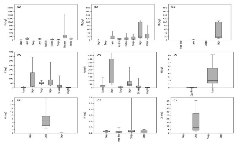
Figure 15: Cation chemistry (a) Ca, (b) Mg, (c) Mn, (d) K, (e) Na. (f) Ni, (g) Cu, (h) Fe, and (i) Zn.

Anion Chemistry

Evaluation of HCO3 concentrations from 119 locations in coastal basins of southwestern Nigeria revealed that HCO3 ranged from 3.6 to 456.28 mg/l with a mean value of 116.98 mg/l (Figure 16a). There are no reference guidelines set up by NSDWQ [125]. Studies on CO3 were not accessed at the time of this study. The two ions are essential to water quality parameters because when CO3 and HC03 are joint with Ca and Mg, they form carbonate hardness. However, if soil concentrates on drying solution, it advances as CaCO3 or MgCO3. Ca and Mg decrease Na concentration levels and the SAR index rise, initiating an alkalizing effect and elevated pH levels. When groundwater analysis shows elevated pH levels, it may indicate the high content of carbonate and bicarbonate ions. Figure 16b presents a synthesis of Cl concentrations in the coastal basin of southwestern Nigeria. Evaluation of Zn in groundwater from 203 sites across the basin revealed that it ranged from 0.12 to 387 mg/l with a mean concentration value of 47.15 mg/l. The NSDWQ [125], has set 250 mg/l as the maximum permissible allowable drinking water limit. Chloride is one of the most common anions found in tap water. Chloride generally combines with Ca, Mg or Na to form various salts: for example, sodium chloride (NaCl) is formed when Cl and Na combine. Chloride occurs naturally in groundwater but is found in high concentrations where seawater and run-off from road salts can make their way into groundwater aquifers. Although Cl is harmless at low levels, groundwater sources having high in NaCl can harm plants if used for gardening or irrigation and give drinking water an unpleasant taste. Over time, NaCl’s high corrosivity will also damage the water system, appliances, and water heaters, causing toxic metals. Nitrate ranged from <0.001 to 50.6 mg/l with a mean value of 8.81 mg/l. There are very few studies on NO2 in coastal basins of southwestern Nigeria (Figure 16c). Akinbile and Yusoff [140]’s environmental impact of leachate pollution on groundwater supplies in Akure, Nigeria, showed that NO2 ranged from 0.7 to 0.9 mg/l with an average value of 0.8 mg/l. The impact of pit latrines on groundwater quality of Fokoslum, Ibadan, Southwestern Nigeria [141], showed that NO2 concentrations vary with pits’ distance. The mean NO2 concentration was 0.12 mg/l at 10.9 meters, 0.05 mg/l at 11.8 meters, 0.12 mg/l at 13.1 meters, 0.21 mg/l at 16.3 meters, 0.22 mg/l at 13.3 meters, 0.19 mg/l at 17.9 meters, 0.23 mg/l at 9.4 meters and 6.1 mg/l at 6.1 meters, respectively. The NO2 from these sites was below the NSDWQ [125] reference limits.

Figure 16d presents a synthesis of PO4 in groundwater from coastal basins of western Nigeria. The PO4 ranged from 0 to 3.5 mg/l with a mean value of 0.65 mg/l. High PO4 in drinking water is not associated with any severe health risks. The presence of PO4 in groundwater is an indicator of anthropogenic pollution since PO4 is mainly derived from organic wastes. The significance of PO4 is mostly linked to eutrophication of surface water bodies. High PO4 and NO3 in water, help plant and algal growths, leading to a variation of diurnal dissolved oxygen, blooms, and littoral slimes [142]. Figure 16e presents a synthesis of SO4 concentrations in groundwater from coastal basins of southwestern Nigeria. The Concentration of SO4 ranged from <0.001 to 1855 mg/l with a mean value of 52.01 mg/l. The NSDWQ [125], has set 100 mg/l as the maximum allowable limit of SO4 in drinking water, even though there is no health risk associated with high ingestion of SO4 drinking water. However, high concentrations of SO4 in drinking water can cause diarrhoea in humans, especially infants. However, adults usually become adapted to high SO4 concentrations after a few days [143].

fig 16

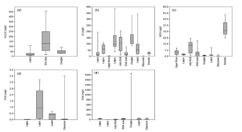
Figure 16: The anion chemistry (a) HCO3, (b) Cl, (c) NO3, (d) PO4, and (e) SO4.

Conclusion

The literature is unanimous about the importance of understanding the hydrogeology and hydrochemistry of groundwater in coastal basins of southwestern Nigeria. Based on the reviewed works, the following remarks can be made:

i. In southwestern Nigeria’s coastal basins, the Abeokuta group is the oldest formation in the area. This group comprised of the Ise, Afowo, and Araromi Formations. Other formations in the basin include the Akinbo and Ilaro formations. Despite the marked spatial variability of these formations, their lithology remains relatively the same.

ii. Also found in this area is the deltaic formation, which contains alluvial deposits. The Ogun Basin is the central coastal basin in western Nigeria, followed by the Osse-Owena Basin. The later has not been fully explored hydrogeologically. The Osun Basin, drained by the Osun River, covers most Osun and Ekiti States parts. This basin is not associated with good groundwater storage, since basement complex rocks underlie it.

iii. These coastal basins were further grouped into the upper surficial aquifer system; and the intermediate aquifer system. Also found in this area is the crystalline Basement Terrain. From the hydrogeologic point of view, unweathered basement rock contains negligible groundwater; though, a significant aquiferous unit can develop within the weathered overburden and fractured bedrock. The general groundwater condition in the area showed that groundwater is very localized.

iv. Groundwater classification based on physical parameters showed mixed results, though groundwater sources are most suitable for drinking.

These basins’ hydrochemistry showed groundwater is relatively good in terms of its suitability for drinking, industrial and agricultural uses. Owing to the increasing urbanization in the area, reasonable measures are required to protect groundwater from overexploitation and pollution.

Acknowledgement

Federal University Birnin kebbi supported this review. Thanks to all anonymous contributors.

References

  1. Olofinlade WS, Daramola S, Olabode OF (2018) Hydrochemical and statistical modeling of groundwater quality in two contrasting geological terrains of southwestern Nigeria. Modeling Earth Systems and Environment 4: 1405-1421.
  2. Arfanuzzaman M, Atiq Rahman A (2017) Sustainable water demand management in the face of rapid urbanization and groundwater depletion for social-ecological resilience building. Global Ecology and Conservation 10: 9-22.
  3. Pahl-Wostl C (2019) The role of governance modes and meta-governance in the transformation towards sustainable water governance. Environmental Science & Policy 91: 6-16.
  4. Rao ND, Min J (2018) Decent Living Standards: Material Prerequisites for Human Wellbeing. Soc Indic Res 138: 225-244. [crossref]
  5. Ficke AD, Myrick CA, Hansen LJ (2007) Potential impacts of global climate change on freshwater fisheries. Reviews in Fish Biology and Fisheries 17: 581-613.
  6. Heathwaite AL (2010) Multiple stressors on water availability at global to catchment scales: understanding human impact on nutrient cycles to protect water quality and water availability in the long term. Freshwater Biology 55: 241-257.
  7. Peters NE, Meybeck (2000) Water Quality Degradation Effects on Freshwater Availability: Impacts of Human Activities. Water International 25: 185-193.
  8. Jamiu AA, Robert M. Kalin, Philippe Sentenac, Ibrahim Hassan, et al. (2020) Assessing the Impact of Climate Change on Groundwater Quality of the Shallow Coastal Aquifer of Eastern Dahomey Basin, Southwestern Nigeria. Water
  9. Md Enamul Huq, Shah Fahad, Zhenfeng Shao, Most Sinthia Sarven, Imtiaz Ali Khan, et al. (2020) Arsenic in a groundwater environment in Bangladesh: Occurrence and mobilization. J Environ Manage [crossref]
  10. Zacchaeus OO (2020) Effects of industrialization on groundwater quality in Shagamu and Ota industrial areas of Ogun State, Nigeria. Heliyon
  11. Asiwaju-Bello YA, Olabode, Ogunsuyi MT (2020) Pollution potential and causative hydrogeochemical processes in unconfined aquifer systems in a typical urban setting: emphasis on recharge and discharge areas. Applied Water Science 10: 1-23.
  12. Fan Feng, Yongfeng Jia,, Yu Yang, Huan Huan, Xinying Lian, et al. (2020) Hydrogeochemical and statistical analysis of high fluoride groundwater in northern China. Environ Sci Pollut Res Int 27: 34840-34861.
  13. Jebreen H (2018) Recharge, geochemical processes and water quality in karst aquifers: Central West Bank, Palestine. Environmental Earth Sciences 77: 1-16.
  14. Muhammad Afnan Talib, Zhonghua Tang, Asfandyar Shahab, Jamil Siddique, Muhammad Faheem, et al. (2019) Hydrogeochemical Characterization and Suitability Assessment of Groundwater: A Case Study in Central Sindh, Pakistan. International Journal of Environmental Research and Public Health 16: 1-21. [crossref]
  15. Osin OA, Yu, S Lin (2017) Oil refinery wastewater treatment in the Niger Delta, Nigeria: current practices, challenges, and recommendations. Environ Sci Pollut Res Int 24: 22730-22740. [crossref]
  16. Ibe KM, PU Agbamu (1999) Impacts of human activities on groundwater quality of an alluvial aquifer: A case study of the Warri River, Delta State, SW, Nigeria. International Journal of Environmental Health Research 9: 329-334.
  17. Emenike PC, CC Nnaji, IT Tenebe (2018) Assessment of geospatial and hydrochemical interactions of groundwater quality, southwestern Nigeria. Environmental Monitoring Assessment 190: 1-17.
  18. Güler C (2012) Assessment of the impact of anthropogenic activities on the groundwater hydrology and chemistry in Tarsus coastal plain (Mersin, SE Turkey) using fuzzy clustering, multivariate statistics and GIS techniques. Journal of Hydrology 414-415: 435-451.
  19. Huang G (2013) Impact of anthropogenic and natural processes on the evolution of groundwater chemistry in a rapidly urbanized coastal area, South China. Sci Total Environ 463-464: 209-21. [crossref]
  20. Ma F (2014) Hydrochemical characteristics and the suitability of groundwater in the coastal region of Tangshan, China. Journal of Earth Science 25: 1067-1075.
  21. Masoud AA (2014) Groundwater quality assessment of the shallow aquifers west of the Nile Delta (Egypt) using multivariate statistical and geostatistical techniques. Journal of African Earth Sciences 95: 123-137.
  22. Badmus GO (2020) Hydrochemical analysis of groundwater quality along the coastal aquifers in part of Ogun Waterside, Ogun State, southwestern Nigeria. Heliyon
  23. Oyeyemi KD, AP Aizebeokhai, MA Oladunjoye (2015) Integrated Geophysical and Geochemical Investigations of Saline Water Intrusion in a Coastal Alluvial Terrain, Southwestern Nigeria. International Journal of Applied Environmental Sciences 10: 1275-1288.
  24. Adelana SMA (2005) The impact of anthropogenic activities over groundwater quality of a coastal aquifer in Southwestern Nigeria. Aquifer Vulnerability and Risk, 2nd 4th International Workshop Congress on the Protection and Management of Groundwater Reggia di Colorno – Parma, 21-22-23 Settembre: p. 1-10.
  25. Awomeso JA, SM Ahmad, AM Taiwo (2020) Multivariate assessment of groundwater quality in the basement rocks of Osun State, Southwest, Nigeria. Environmental Earth Sciences 79: 1-9.
  26. A AJ, TA O (2013) Assessment of Groundwater Quality in Abeokuta Southwestern, Nigeria. Research Inventory: International Journal of Engineering and Science 2: 21-31.
  27. Yusuf MA, TA Abiye (2019) Risks of groundwater pollution in the coastal areas of Lagos, southwestern Nigeria. Groundwater for Sustainable Development
  28. Aizebeokhai AP, KD Oyeyemi, ES Joel (2016) Groundwater potential assessment in a sedimentary terrain, southwestern Nigeria. Arabian Journal of Geosciences
  29. Akaegbobi IM, GO Ogungbesan (2016) Geochemistry of the Paleocene limestones of Ewekoro Formation, Eastern Dahomey Basin, Southwestern Nigeria: Implication on Provenance and Depositional Conditions. Ife Journal of Science 18: 669-684.
  30. Ola-Buraimo AO (2014) Biostratigraphy of the Campano-Maastrichtian Uzeeba Shale deposit, Dahomey Basin Southwestern Nigeria. Elixir Geoscience 69: 22812-22818.
  31. Ola-Buraimo OA (2012) Palynological Investigation of a Type Section of Early Maastrichtian Arimogija – Okeluse Shale Sequence, Dahomey (Benin) Embayment, Southwestern Nigeria. International Journal of Science & Emerging Technologies 3: 37-45.
  32. Offodile ME (2002) Groundwater Study and Development in Nigeria, second edition, Mecon Geology and Eng. Services Ltd. Pg: 1- 453.
  33. Oli IC (2019) A Review of the Geology and Mineral Resources of Dahomey Basin, Southwestern Nigeria. International Journal of Environmental Sciences & Natural Resources 21: 1-5.
  34. Obomighie PO, JO Gwegwe, AG Oluwadebi (2016) Petrographic Studies and Paleoenvironmental Reconstruction of Some Outcropping Sediments in Parts of Eastern Dahomey Basin, South-Western, Nigeria. IOSR Journal of Applied Geology and Geophysics 4: 9-15.
  35. Nton NE, PR Ikhane, MN Tijani (2009) Aspect of rock-eval studies of the Maastrichtian-Eocene sediments from subsurface, in the eastern Dahomey basin southwestern Nigeria. European Journal of Scientific Research 25: 417-427.
  36. Olabode, S.O. and M.Z. (2016) Mohammed, Depositional Facies and Sequence Stratigraphic Study in Parts of Benin (Dahomey) Basin SW Nigeria: Implications on the Re-Interpretation of Tertiary Sedimentary Successions. International Journal of Geosciences 7: 210-228.
  37. Olabode SO, JA Adekoya (2008) Seismic stratigraphy and development of Avon canyon in Benin (Dahomey) basin, southwestern Nigeria. Journal of African Earth Sciences 50: 286-304.
  38. Olatinsu O (2017) Lithotype characterizations by Nuclear Magnetic Resonance (NMR): A case study on limestone and associated rocks from the eastern Dahomey Basin, Nigeria. Journal of African Earth Sciences 129: 701-712.
  39. Okosun EA (1990) A review of the Cretaceous stratigraphy of the Dahomey Embayment, West Africa. Cretaceous Research 11: 17-27.
  40. Adeoti L, OM Alile, O Uchegbulam (2010) Geophysical investigation of saline water intrusion into freshwater aquifers: A case study of Oniru, Lagos State. Scientific Research and Essays 5: 248-259.
  41. Mohammed S, M Opuwari, S Titinchi (2020) Source rock evaluation of Afowo clay type from the Eastern Dahomey Basin, Nigeria: insights from different measurements. Sci Rep
  42. Adeoye JA (2020) Geochemistry and paleoecology of shales from the Cenomanian-Turonian Afowo formation Dahomey Basin, Nigeria: Implication for provenance and paleoenvironments. Journal of African Earth Sciences
  43. Nton ME, PR Ikhane, MN Tijani (2009) Aspect of Rock-Eval Studies of the Maastrichtian-Eocene Sediments from Subsurface, in the Eastern Dahomey Basin Southwestern Nigeria. European Journal of Scientific Research 25: 417-427.
  44. Akaegbobi IM, GO Ogungbesan, JE Ogala (2011) Carbonate Microfacies and Major Element Content of The Paleocene – Eocene Sections Exposed at the Sagamu Quarry, Eastern Dahomey Basin, Nigeria. Global Journal of Geological Sciences 9: 241-251.
  45. PR I (2012) Petrography and Geochemical Appraisal of Afowo Sandstone Facies, Dahomey Basin, Southwestern Nigeria. Chemistry and Materials Research 2: 50-59.
  46. Adelana, SMA (2008) An overview of the geology and hydrogeology of Nigeria. Chapter 11. 15(11): pg: 171-198.
  47. Adekeye OA (2019) Biostratigraphic Analysis of the Cretaceous Abeokuta Group in the Eastern Dahomey Basin, Southwestern Nigeria. Journal of African Earth Sciences 152: 171-183.
  48. Joel ES (2019) Integration of aeromagnetic and electrical resistivity imaging for groundwater potential assessments of coastal plain sands area of Ado-Odo/Ota in southwest Nigeria. Groundwater for Sustainable Development
  49. Osinowo OO, AO Akanji, AI Olayinka (2014) Application of high-resolution aeromagnetic data for basement topography mapping of Siluko and environs, southwestern Nigeria. Journal of African Earth Sciences 99: 637-651.
  50. Aladejana JA, AO Talabi (2013) Assessment of Groundwater Quality in Abeokuta Southwestern, Nigeria. Research Inventy: International Journal of Engineering And Science 2: 21-31.
  51. Oyedele KF, EI Momoh (2009) Evaluation of Seawater Intrusion in Freshwater Aquifers in a Lagoon Coast: A Case Study of the University of Lagos Lagoon, Akoka, Nigeria. Report and Opinion 1: 1-12.
  52. Adeyemi GO (2013) Geophysical and Sedimentological Characterization of a Tar Sand Rich Area in South-western Nigeria. Journal of Environment and Earth Science 2: 71-83.
  53. Akinmosin A, AO Shoyemi (2010) Technical Feasibility of Direct Application of the Nigerian Tar Sand Deposits as Road Asphalt. The Pacific Journal of Science and Technology 11: 526-536.
  54. Adepelumi A, B Ako, T Ajayi (2001) Groundwater contamination in the basement-complex area of Ile-Ife, southwestern Nigeria: A case study using the electrical-resistivity geophysical method. Hydrogeology Journal 9: 611-622.
  55. Oyedele KF, S Oladele, C Okoh (2012) Geo-Assessment of subsurface conditions in Magodo Brook Estate, Lagos, Nigeria. International Journal of Advanced Scientific and Technical Research 2: 731-741.
  56. Oteri, UO, RA Ayeni (2016) The Lagos Mega City: Water Megacities and Global Change. Available at: http://eaumega.org/wp-content/uploads/2016/05/EN-Lagos-Monograph.pdf,: pg: 1-36.
  57. Amajor LC (1991) Aquifers in the Benin Formation (Miocene Recent), Eastern Niger Delta, Nigeria: Lithostratigraphy, Hydraulics, and Water Quality. Environmental Geology and Water Science 17: 85-101.
  58. Oomkens E (1974) Lithofacies relations in the Late Quaternary Niger Delta complex. Sedimentology 21: 195-222.
  59. Reijers TJA, SW Petters, CS Nwajide (1997) The Niger Delta Basin. African Basins. Sedimentary Basins of the World, 3 edited by R.C. Selley (Series Editor: K.J. Hsti) p. 151-172.
  60. Adeyemi O, F Olutoyin, O Olumide (2020) Downstream hydraulic geometry across headwater channels in Upper Ogun River Basin, Southwestern Nigeria. African Geographical Review 39: 345-360.
  61. Eludoyin AO, AO Adewole (2019) A remote sensing-based evaluation of an ungauged drainage basin in Southwestern Nigeria. International Journal of River Basin Management 18: 307-319.
  62. Olusola A (2020) Morphologic and hydraulic variability of small bedrock and alluvial channels in relation to lithological controls, Upper Ogun River Basin, Southwestern Nigeria. Physical Geography 41: 537-557.
  63. Oke MO (2015) Comparative analysis of groundwater recharge estimation value obtained using empirical methods in Ogun and Oshun river basins. Ife Journal of Science 17: 53-63.
  64. Ikhile CI (2012) The Impacts of Climate Change on the Discharge of OsseOssiomo River Basin, South Western Nigeria under Different Climatic Scenarios. An International Journal of Science and Technology Bahir Dar, Ethiopia 1: 1-13.
  65. Catherine II, O Lekan (2007) Application of GIS in land-use studies in the Osse-Ossiomo River basin, Nigeria. Remote Sensing for Environmental Monitoring and Change Detection (Proceedings of Symposium HS3007 at IUGG2007, Perugia, July 2007). IAHS Publ. 316: 245-251.
  66. Solomon O, O Prince (2013) Flood Frequency Analysis of Osse River Using Gumbel’s Distribution. Civil and Environmental Research 3: 55-59.
  67. Oke MO (2013) Comparative Analysis of Empirical Formulae Used in Groundwater Recharge in Ogun – Oshun River Basins. Journal of Scientific Research & Reports 2: 692-710.
  68. Adepelumi AA (2009) Delineation of saltwater intrusion into the freshwater aquifer of Lekki Peninsula, Lagos, Nigeria. Environmental Geology 56: 927-933.
  69. Bayewu OO (2017) Geophysical evaluation of groundwater potential in part of southwestern Basement Complex terrain of Nigeria. Applied Water Science 7: 4615-4632.
  70. Lateef TA (2012) Geophysical Investigation For Groundwater Using Electrical Resistivity Method – A Case Study Of Annunciation Grammar School, Ikere Lga, Ekiti State, South-Western Nigeria. IOSR Journal of Applied Physics 2: 1-6.
  71. Fashae OA (2014) Delineation of groundwater potential zones in the crystalline basement terrain of SW-Nigeria: an integrated GIS and remote sensing approach. Applied Water Science 4:19-38.
  72. Egbinola CN (2014) Amanambu, Christiana Ndidi Egbinola* and Amobichukwu Chukwudi Amanambu. SpringerPlus 3: 1-6.
  73. Akinyemi FO (2013) An assessment of land-use change in the Cocoa Belt of south-west Nigeria. International Journal of Remote Sensing 34: 2858-2875.
  74. DeSimone LA, JP Pope KM (2020) Ransom, Machine-learning models to map pH and redox conditions in groundwater in a layered aquifer system, Northern Atlantic Coastal Plain, eastern USA. Journal of Hydrology: Regional Studies
  75. Laluraj CM, G Gopinath (2006) Assessment on seasonal variation of groundwater quality of phreatic aquifers – a river basin system. Environ Monit Assess 117: 45-57.
  76. Takem GE (2015) Acidification of shallow groundwater in the unconfined sandy aquifer of the city of Douala, Cameroon, Western Africa: implications for groundwater quality and use. Environmental Earth Sciences 74: 6831-6846.
  77. Douglas TM, LS Robert (2015) Corrosion Control by Deposition of CaCO₃ Films: Part 1, A Practical Approach for Plant Operators. American Water Works Association 69: 592-599.
  78. Marc, E., R.S. Michael, and E.M. Travis (1996) Alkalinity, pH, and copper corrosion by-product release. American Water Works Association.
  79. Gouda VK (1970) Corrosion and Corrosion Inhibition of Reinforcing Steel: I. Immersed in Alkaline Solutions. British Corrosion Journal 5:198-203.
  80. Melidis P (2007) Corrosion control by using indirect methods. Desalination 213: 152-158.
  81. Asare-Donkor NK, DD Wemegah, AA Adimado (2013) Chemical Analysis of Freshwater Bodies in the Kumasi Metropolis and Its Environs, Ghana. Journal of Environment and Earth Science 3: 37-45.
  82. Bacha AA, MI Durrani, PI Paracha (2010) Physical and Bacteriological Characteristics of Drinking Water of Peshawar. Pakistan Journal of Nutrition 9: 1028-1033.
  83. Haziq MA, NA Qani (2017) Physiochemical Assessment of Drinking Water Quality in Kandahar City, Afghanistan. International Journal of Innovative Science and Research Technology 2: 7-24.
  84. Timothy AO, KH M (1978) The effect of pH and hardness metal ions on the competitive interaction between trace metal ions and inorganic and organic complexing agents found in natural waters. Water Research 12: 703-711.
  85. Karthikeyan S, PLR Palaniappan, S Sabhanayakam (2007) Influence of pH and water hardness upon nickel accumulation in edible fish Cirrhinus mrigala. Journal of Environmental Biology 28: 489-492.
  86. Ruiz-Ramirez J (2005) Relationship between water content, NaCl content, pH and texture parameters in dry-cured muscles. Meat Sci 70: 579-587.
  87. Florides G, S Kalogirou (2007) Ground heat exchangers—A review of systems, models and applications. Renewable Energy 32: 2461-2478.
  88. Green TR (2011) Beneath the surface of global change: Impacts of climate change on groundwater. Journal of Hydrology 405: 532-560.
  89. Keery J (2007) Temporal and spatial variability of groundwater-surface water fluxes: Development and application of an analytical method using temperature time series. Journal of Hydrology 336: 1-16.
  90. Alva G, Y Lin, G Fang (2018) An overview of thermal energy storage systems. Energy 144: 341-378.
  91. Zhu S (2020) Using seasonal temperature difference in underground surrounding rocks to cooling ventilation airflow: A conceptual model and simulation study. Energy Science & Engineering 8: 3457-3475.
  92. Boulton AJ, PJ Hancock (2006) Rivers as groundwater-dependent ecosystems: a review of degrees of dependency, riverine processes and management implications. Australian Journal of Botany 54: 133-144.
  93. Humphreys WF (2008) Hydrogeology and groundwater ecology: Does each inform the other?. Hydrogeology Journal 17: 5-21.
  94. Strona G (2019) AQUA LIFE Software: A New Tool for a Standardized Ecological Assessment of Groundwater Dependent Ecosystems. Water 11: 1-17.
  95. Hayashi M (2004) Temperature-electrical conductivity relation of water for environmental monitoring and geophysical data inversion. Environmental Monitoring and Assessment 96: 119-128.
  96. Beddows PA (2007) Decoupled fresh–saline groundwater circulation of a coastal carbonate aquifer: Spatial patterns of temperature and specific electrical conductivity. Journal of Hydrology 346: 18-32.
  97. Sargaonkar A, V Deshpande (2003) Development of an overall index of pollution for surface water based on a general classification scheme in Indian context. Environmental Monitoring and Assessment 89: 43-67.
  98. Zakir HM (2017) Quality and Metallic Pollution Level in Surface Waters of an Urban Industrialized City: A Case Study of Chittagong City, Bangladesh. Journal of Industrial Safety Engineering 4: 9-18.
  99. Güler C, M Alpaslan (2009) Mineral content of 70 bottled water brands sold on the Turkish market: Assessment of their compliance with current regulations. Journal of Food Composition and Analysis 22: 728-737.
  100. Karavoltsos S (2008) Evaluation of the quality of drinking water in regions of Greece. Desalination 224: 317-329.
  101. Naveen BP (2017) Physico-chemical and biological characterization of urban municipal landfill leachate. Environmental Pollution 220: 1-12.
  102. Rubenowitz-LundinKevin, E. and K.M. Hiscock, Water Hardness and Health Effects. In: Essentials of Medical Geology. Revised Edition. Eds: O. Selinus. Springer Dordrecht Heidelberg New York London, 2013: pg: 1-808.
  103. Ghernaout (2018) Combining lime softening with alum coagulation for hard Ghrib dam water conventional treatment. International Journal of Advanced and Applied Sciences 5: 61-70.
  104. Richards CS (2018) A 21st-Century Perspective on Calcium Carbonate Formation in Potable Water Systems. Environmental Engineering Science 35: 143-158.
  105. Farrell C (2018) Turbidity composition and the relationship with microbial attachment and UV inactivation efficacy. Sci Total Environ 624: 638-647.
  106. Edwards AC, PJA (2008) Withers, Transport and delivery of suspended solids, nitrogen and phosphorus from various sources to freshwaters in the UK. Journal of Hydrology 350: 144-153.
  107. Appleyard, S, T Cook (2008) Reassessing the management of groundwater use from sandy aquifers: acidification and base cation depletion exacerbated by drought and groundwater withdrawal on the Gnangara Mound, Western Australia. Hydrogeology Journal 17: 579-588.
  108. Mushtaq N (2018) Hydrogeochemical and isotopic evaluation of groundwater with elevated arsenic in alkaline aquifers in Eastern Punjab, Pakistan. Chemosphere 200: 576-586.
  109. Sabarathinam C, H Bhandary, A Al-Khalid (2020) Tracing the evolution of acidic hypersaline coastal groundwater in Kuwait. Arabian Journal of Geosciences 13: 1-19.
  110. Ayolabi EA, AF Folorunso, OT Kayode (2013) Integrated Geophysical and Geochemical Methods for Environmental Assessment of Municipal Dumpsite System. International Journal of Geosciences 4: 850-862.
  111. Awomeso JA (2010) Studies on the pollution of waterbody by textile effluents in.Lagos, Nigeria. Journal of Applied Sciences in Environmental Sanitation 5: 353-359.
  112. Omale DO, EO Longe (2008) An assessment of the impact of abattoir effluents on River Illo, Ota, Nigeria. Journal of Environmental Science and Technology 2: 56-64.
  113. Siljic Tomic A (2018) A linear and non-linear polynomial neural network modelling of dissolved oxygen content in surface water: Inter- and extrapolation performance with inputs’ significance analysis. Sci Total Environ 610-611: 1038-1046.
  114. Voisin J (2018) Aquifer recharge with stormwater runoff in urban areas: Influence of vadose zone thickness on nutrient and bacterial transfers from the surface of infiltration basins to groundwater. Sci Total Environ 637-638: 1496-1507.
  115. Ward, C.P. and R.M. Cory (2020) Assessing the prevalence, products, and pathways of dissolved organic matter partial photo-oxidation in Arctic surface waters. Environ Sci Process Impacts 22: 1214-1223.
  116. Baldock JA, JO Skjemstad (2000) Role of the soil matrix and minerals in protecting natural organic materials against biological attack. Organic Geochemistry 31: 697-710.
  117. Chu L (2009) Progress and perspectives of sludge ozonation as a powerful pretreatment method for minimization of excess sludge production. Water Res 43: 1811-22.
  118. Wali SU, N Alias, SB Harun (2020) Quality reassessment using water quality indices and hydrochemistry of groundwater from the Basement Complex section of Kaduna Basin, NW Nigeria. SN Applied Sciences
  119. Wali, SU, N Alias, BH Sobri (2020) Hydrogeochemical evaluation and mechanisms controlling groundwater in different geologic environments, Western Sokoto Basin, Northwestern Nigeria. SN Applied Sciences
  120. Longe, EO, LO Enekwechi (2007) Investigation on potential groundwater impacts and influence of local hydrogeology on natural attenuation of leachate at a municipal landfill. International Journal of Environmental Science and Technology 4: 133-140.
  121. Izah, SC, AL Srivastav (2015) Level of arsenic in potable water sources in Nigeria and their potential health impacts: A review. Journal of Environmental Treatment Techniques 3:15-24.
  122. WHO, Guidelines for drinking‑water quality: Fourth edition incorporating the first addendum. WHO Library Cataloguing-in-Publication Data. World Health Organization Geneva 2018: 631.
  123. Odukoya AM, AF Abimbola (2010) Contamination assessment of surface and groundwater within and around two dumpsites. International Journal of Environmental Science and Technology 7: 367-376.
  124. WHO, Guidelines for drinking-water quality: First Addendum to Third Edition Recommendations. World Health Organization Geneva, 2006 1: 595.
  125. NSDWQ, Nigerian Standard for Drinking Water Quality: Nigerian Industrial Standard NIS 554. Standards Organisation of Nigeria, 2007: 30.
  126. Majolagbe AO, AA Kasali, LO Ghaniyu (2011) Quality assessment of groundwater in the vicinity of dumpsites in Ifo and Lagos, Southwestern Nigeria. Advances in Applied Science Research 2: 289-298.
  127. Adekunle IM (2007) Assessment of Groundwater Quality in a Typical Rural Settlement in Southwest Nigeria. International Journal of Environmental Research and Public Health 4: 307-318.
  128. Gbadebo AM (2012) Groundwater fluoride and dental fluorosis in southwestern Nigeria. Environ Geochem Health 34: 597-604.
  129. Egbinola CN, AC Amanambu (2014) Groundwater contamination in Ibadan, South-West Nigeria. SpringerPlus 3: 1-6.
  130. Jha SK (2013) Fluoride in groundwater: toxicological exposure and remedies. Journal of Toxicology and Environmental Health, Part B 16: 52-66.
  131. Adimalla N, S Venkatayogi (2016) Mechanism of fluoride enrichment in groundwater of hard rock aquifers in Medak, Telangana State, South India. Environmental Earth Sciences 76:1-10.
  132. Jha SK (2013) Fluoride in groundwater: toxicological exposure and remedies. J Toxicol Environ Health B Crit Rev 16: 52-66.
  133. Singh CK (2011) Application of GWQI to Assess Effect of Land Use Change on Groundwater Quality in Lower Shiwaliks of Punjab: Remote Sensing and GIS-Based Approach. Water Resources Management 25: 1881-1898.
  134. Olowe B, J Oluyege, O Famurewa (2016) An Assessment of Drinking Water Quality Using Water Quality Index in Ado-Ekiti and Environs, Nigeria. American Chemical Science Journal 12:1-7.
  135. Oyeyemi KD, AP Aizebeokhai, HI Okagbue (2017) Geostatistical exploration of dataset assessing the heavy metal contamination in Ewekoro limestone, Southwestern Nigeria. Data Brief 14: 110-117.
  136. Gbadebo AM, AM Taiwo, AJ Adeola (2013) Assessment of Dissolved Silica Content of Groundwater from Southwestern Nigeria. Journal of Human Ecology 43: 273-279.
  137. Ityel D, Groundwater: Dealing with iron contamination. Available at https://www.sciencedirect.com/science/article/abs/pii/S001518821170043X. Retrieved on 09/09/2020, 2011: 1-3.
  138. Noffke A (2012) Benthic iron and phosphorus fluxes across the Peruvian oxygen minimum zone. Limnology and Oceanography 57: 851-867.
  139. Spuhler D, J Andrés Rengifo-Herrera, C Pulgarin (2010) The effect of Fe2+, Fe3+, H2O2 and the photo-Fenton reagent at near-neutral pH on the solar disinfection (SODIS) at low temperatures of water containing Escherichia coli K12. Applied Catalysis B: Environmental 96: 126-141.
  140. Akinbile CO, MS Yusoff (2011) Environmental Impact of Leachate Pollution on Groundwater Supplies in Akure, Nigeria. International Journal of Environmental Science and Development 2: 81-86.
  141. Ahaneku IE, PA Adeoye (2014) Impact of Pit Latrines on Groundwater Quality of Fokoslum, Ibadan, Southwestern Nigeria. British Journal of Applied Science & Technology 4: 440-449.
  142. EPA, Parameters of water quality: Interpretation and Standards. An Ghniomhaireacht um Chaomhnu Comhshaoil. Ireland. 2001 1-132.
  143. Miao Z (2012) Sulfate reduction in groundwater: characterization and applications for remediation. Environ Geochem Health 34: 539-50.
fig 1

Formulation of Rivastigmine, a Liquid Drug Substance, for Use in a Simulating Study of Hollow Microstructured Transdermal Delivery System

DOI: 10.31038/JPPR.2020333

Abstract

Rivastigmine, used in the treatment of Alzheimer’s Disease, is in liquid state at controlled room temperatures. This project was aimed at developing a 0.5-mL isotonic liquid containing rivastigmine with the choice of 0.9% NaCl or 5% Dextrose Solutions for Injection as a simulating study to formulate a liquid dosage form per description of 3M hollow microneedles (https://multimedia.3m.com/mws/media/1004089O/solid-microstructured-transdermal-system-smts-sell-sheet.pdf). The surfactants were compared among Span 20, Span 80, Tween 40 and Tween 80 with benzyl alcohol or chlorobutanol as a preservative. Those formulations which formed microemulsions were further studied for stability at 4°C and 25°C up to one month. HPLC confirmed that there were no drug losses among the four microemulsions. Based on zeta potential and particle size analysis, Tween 80 with benzyl alcohol in 0.9 % NaCl is the best project formulation.

Keywords

Benzyl alcohol, chlorobutanol, Hollow Microstructured Transdermal System (hMTS), microneedles, rivastigmine, Tween and Span

Introduction

Alzheimer’s disease is an irreversible, progressive neurodegenerative disorder subsequently becoming a common cause of death [1]. Alzheimer’s is the most common cause of dementia affecting an estimated 5.8 million people in the United States [1]. In 2018, the approximate cost of caring for people with Alzheimer’s disease and other dementias was $290 billion USD, making it a huge economic burden for both patients’ families and our society and leading to a major public health problem. It is a huge economic burden for patients’ families and our society. Unfortunately, there has not been an effective treatment for Alzheimer’s disease thus far. One of the reasons is that the exact mechanism of disease development is still unclear. Acetylcholinesterase inhibitors such as donepezil, rivastigmine and galantamine, and N-methyl D-asparate receptor antagonist, and memantine are therapeutic agents. Among them, rivastigmine has the advantage of inhibiting both acetylcholinesterase (AChE) and butyrylcholinesterase (BuChE). It is also superior to the aforementioned other drugs in having two US FDA approved commercial dosage forms, that is oral capsules and transdermal patches (Table 1) [2,3]. Unfortunately, nausea and vomiting have been reported by patients taking rivastigmine oral dosage form [4]. Transdermal delivery system has a better tolerability and more efficacy compared to oral capsules [5] and enables patients who have difficulties in swallowing to take medicine more easily, and less frequently (once daily, Table 1b) [6]. However, it was reported that transdermal patch may cause skin irritation when a 24-h patch is worn. Therefore, this study focuses on the feasibility of formulating rivastigmine for use of microneedle administration and formulation characterizations. Microneedle has been gathering attention on their merits, including shorter time to reach Cmax and penetrating more drugs, especially macromolecules, than the transdermal patch dosage form [7].

Table 1: Rivastigmine dosage forms on the market: (a) oral capsules, and (b) extended release transdermal films [2,3].

(a) Oral capsules

Strength Manufacturers Applicant Holder
EQ 1.5, 3, 4.5, 6 mg BASE Brand name product Novartis
EQ 1.5, 3, 4.5, 6 mg BASE Generic products Alembic; Apotex; Aurobindo; Cadila; Chartwell; Dr. Reddy’s; Macleods; Orchid; Sun; Watson

(b) Extended release transdermal film

Strength Manufacturers Applicant Holder
4.6, 9.5, 13.3 mg/24 h Brand name product Novartis
4.6, 9.5, 13.3 mg/24 h Generic products Alvogen malta operations;

Amneal; Mylan; Zydus

Microneedles devise a pain-free penetration feature (minimally invasive device which pierces through the stratum corneum without touching the nerve endings and capillaries). Its other merits are avoidance of the first-pass, improvement of skin permeability and permeation, the delivery of both small and large molecules, achieve stable plasma concentrations for up to 7 days and possibly improvement of bioavailability. There are four subtypes of microneedles: solid, coated, dissolving, and hollow [8-10].

Colloidal Dispersions, Emulsions and Microemulsions

Colloids are heterogeneous mixture systems. Colloidal dispersion is characterized by their particle sizes and shapes. A particle size ranged between 1 nm and 1 μm makes the properties of colloids fall between solution and suspensions. Whether their particles are small enough to separate on standing or are large enough to scatter light (a phenomenon called Tyndall effect, which makes the liquid’s appearance cloudy or opaque) depends on the particle size. Therefore, colloidal dispersions are further divided into molecular colloids (solutions), association colloids and dispersion colloids [11]. Emulsions are composed of two or more immiscible liquids and suitable emulsifying agent(s), which appear milky and nontransparent because of the different optical refraction of the components. Depending on the hydrophilic and lipophilic characters, emulsions may be divided into oil in water (O/W) and water in oil (W/O) subtypes. In addition to these, multiple phases of emulsions exist as W/O/W and O/W/O microemulsions. Emulsions are kinetically stable but thermodynamically unstable based on their dispersed state and the corresponding high interfacial energy. On the other hand, microemulsions are fundamentally different from emulsions in terms of appearance, structure, and properties, which are considered between micellar solution and emulsions. Their appearances vary from transparent to opalescent, moderately viscous, and optically isotropic. Microemulsions are thermodynamically stable [11,12].

Materials

Rivastigmine (1 g and 0.5 g HY-17368 in two separate orders; liquid state in controlled room temperature) was obtained from MedChem Express (Monmouth Junction, NJ). 5 % Dextrose (also known as D5W, Lot J4J577) and 20 mL syringes were acquired from Cardinal Health (Dublin, OH). Sodium chloride (Lot: 284929), Tween 40 (polyxyethylene sorbitan monopalmitate, Lot: D5ZONHK, TGI Tokyo, Japan), methanol and 0.2 micron VWR syringe filters were ordered from VWR International (Randor, PA). Span 20 (Sorbitan monolaurate, Lot: C1885020), Span 80 (sorbitan monooleate, Lot: C182545), Tween 80 (polysorbate, Lot: C188508), benzyl alcohol (Lot: C171703), chlorobutanol, and sodium phosphate dibasic were bought from PCCA (Houston, TX).

Methods

Determination of High Performance Liquid Chromatographic (HPLC) Column

USP43-NF38 2020 recommended to assay rivastigmine and its tartrate salt by using Symmetry C18, Nova Pak C18, and Spherisorb C8 columns [13]. Buffer was first prepared as 8.9 g/L of dibasic sodium phosphate dihydrate in water (0.05 M). Mobile phase was the mixture of methanol and Buffer (0.05M sodium phosphate dibasic) in 58:42 v/v ratio. The solution was let cool to controlled room temperature before the pH adjustment to the value of 8.45 using phosphoric acid. The LC assay conditions were flow rate of 1.0 mL/min, and column temperature at 40°C. The detection wavelength was chosen at 214 nm for all study LC columns with run time at 20 minutes initially. When no impurities were seen, the run time was reduced to 15 minutes or shorter to avoid the generation of biohazard wastes from the prolonged use of mobile phase containing methanol.

Standard Curve

Ten mL of rivastigmine (which density is 1.0 g/mL) initially placed in a volumetric flask to determine its weight. A sufficient amount of the mobile phase was then added to make it into 10 mL as the stock solution, which has a concentration of 1 mg/mL (because the density of rivastigmine is 1 g/mL). This stock solution was further diluted 5-fold with mobile phase each time for sequentially six times with the eighth sample only being diluted two-fold from the seventh sample. One mL of each was transferred into a HPLC vial for assay injection. Accuracy is determined based on how close a measured value is to the actual (true) value. One of the actual (true value) may rely on the use of USP Reference Standard for comparison. Precision is determined based on how close the measured values are to each other. Since Rivastigmine USP Reference Standard was not available for the free base form to report Accuracy (but available as Rivastigmine Tartrate). This project reported the Precision instead. The HPLC conditions were as the follows: wavelength at 214 nm; flow rate 1.0 mL/min; run time 12 min; column temperature 40°C.

Formulation Preparation

3M Hollow Microstructured Transdermal System (hMTS) is an integrated device containing actuator, glass injection cartridge, delivery spring, adhesive, hollow microstructured array and application spring with information available at 3M, St. Paul, MN [12]. Each glass cartridge may house 0.5 mL to 2 mL of intradermal delivery solution (Figure 1a and 1b). In this project, 4.6 μL of rivastigmine (that is 4.6 mg) was selected to develop into 0.5 mL of liquid dosage form as a single dose. As aforementioned, rivastigmine is in liquid state at controlled room temperature, its density is 1.0 g/mL. Therefore, rivastigmine was measured by volume, instead of weight in this project. Suitable excipients such as solution for injection, surfactant and preservative were added into the final volume of 0.5046 mL, which is within the glass cartridge capacity between 0.5 mL to 2 mL. The selection of excipients such as Solutions for Injection, surfactants, and preservatives are briefly described as follows. Isotonic 0.9% saline and 5% dextrose (D5W) were chosen as Solutions for Injection. Since rivastigmine is lipophilic and in liquid state at controlled room temperature (23 ± 2°C), four surfactants (Span 20; Span 80; Tween 40 and Tween 80 (Figure 2) were added respectively to check compatibility. In addition, two preservatives (benzyl alcohol or chlorobutanol) were included. Each formulation in the saline group was composed of 0.9 g of NaCl, 5.0 g of surfactants and 1.0 g of benzyl alcohol (or 0.5g of chlorobutanol) in 100 mL final volume. The D5W group contained 5.36 g of surfactants, 1.0 g of benzyl alcohol (or 0.5 g of chlorobutanol) with sufficient amount of D5W in the total of 100 mL final volume. After mixing, the degree of transparency vs. cloudiness of all formulations were visually observed to determine candidacy for further testing. Rivastigmine 0.92 mL was taken and mixed with each 100 mL of liquid to assess particle size, zeta potential and conduct HPLC.

fig 1

Figure 1: Hollow Microneedle Transdermal System (hMTS): (a) 3M device, (b) scheme showed the inside view of the integrated device, and (c) polymer microneedle array with 12 hollow microneedles, each approximately 1500 µm [12].

fig 2

Figure 2: The appearance of surfactants from left to right: Span 20 (HLB 8.6), Span 80 (HLB 4.0), Tween 40 (HLB 15.6) and Tween 80 (HLB 15.0).

Visual Characterization

The miscibilities of resultant formulations after rivastigmine mixed with one of the two Solutions for Injection, one of the four surfactants and one of the two preservatives were visually observed.

Particle Size Analysis and Zeta Potential

Rivastigmine (9.2 μL, density 1 g/mL) was added to the aforementioned different blank formulations into the total volume of 2 mL for each. The formulations were analyzed by the NanoBrook 90 Plus Particle Sizer. The refractive indexes of rivastigmine, Span 20, Tween 40, Tween 80, benzyl alcohol, and chlorobutanol used in particle size analysis were 1.518, 1.474, 1.470, 1.473, 1.539, and 1.491, respectively (Refractive index of a medium is the ratio of the speed of light in vacuum to the speed of light in the medium. Therefore, it has no units). The zeta potentials of formulations were analyzed using NanoBrook 90 Plus Zeta Potential Reader.

One-Month Stability Study

Each formulation sample containing 4.6 μL of rivastigmine (equivalent to 4.6 mg) was subject to HPLC assay as Time 0 samples. The LC method was adopted from USP-NF 2020 [13]. One half mL of this liquid plus 4.6 μL (4.6 mg) of rivastigmine was then taken into an amber vial and crimped with an aluminum cap (as a single dose) and stored at 4°C and 25°C respectively (n = 3) for one month prior to HPLC assay to determine the drug loss and compare the stabilities among formulation candidates.

Statistics

AUCs obtained from HPLC were statistically assessed by one way or two way ANOVA tests when normality and equal variance were met. Kruska-Wallis test was used if normality and equal variance were not met. Tukey as postdoc was used to compare the three groups. Population differences are considered significant at P < 0.05.

Results

Visual Observation

When using D5W as the Solution for Injection and mixed with one of the four surfactants, the Span 20 group looked homogeneous, but Span 80 appeared as heterogeneous. Tween 40 formed a yellowish clear solution. Tween 80 was a pale yellowish clear solution. Therefore, Span 80 was excluded from further experiments. Next, one of the two preservatives was added into these formulations. Preservative (either benzyl alcohol and chlorobutanol) in Span 20 formed milky microemulsion (Table 2). Benzyl alcohol with Tween 40 resulted in colloidal dispersion, while chlorobutanol formed microemulsion. Like Tween 40, chlorobutanol with Tween 80 formed microemulsion but benzyl alcohol had colloidal dispersion. Using 0.9 % NaCl for Solution for Injection, in contrast with D5W, Span 20 and Span 80 were heterogeneous and immiscible. From these results, they were eliminated from the formulation. Tween 40 in 0.9% NaCl was a yellowish clear solution. When benzyl alcohol was added as a preservative, it formed yellowish colloidal dispersion, while chlorobutanol formed precipitations. Tween 80 in 0.9% saline was also a clear solution. When either preservative was added to Tween 80, they formed clear microemulsion.

Table 2: Miscibilities of surfactants and preservatives in D5W or 0.9% NaCl Solution.

Surfactant

Preservative

D5W

0.9% NaCl

Span 20 Benzyl Alcohol

Emulsion

Non-miscible

Chlorobutanol

Emulsion

Non-miscible

Span 80

Non-miscible

Non-miscible

Tween 40 Benzyl Alcohol

Colloidal dispersion

Colloidal dispersion

Chlorobutanol

Microemulsion

Precipitation

Tween 80 Benzyl Alcohol

Colloidal dispersion

Microemulsion

Chlorobutanol

Microemulsion

Microemulsion

Particle Size and Zeta Potential Analyses

Span 20 with each preservative in D5W, Tween 80 with chlorobutanol in D5W and Tween 80 with each preservative in 0.9% NaCl were good candidates only in terms of particle sizes (Table 3). Among D5W, Tween 40 was significant different with Span 20 and Tween 80. However, there was no significant difference by using one or the other preservatives. Within benzyl alcohol in D5W, Span 20 and Tween 40 showed significantly different. Nevertheless, Span 20 and Tween 80 or Tween 40 and Tween 80 showed no difference. Furthermore, within chlorobutanol, between Tween 40 and Span 20 or Tween 80 showed a significant difference. Among the sample groups made of 0.9 % NaCl as Solution for Injection, there is no significant difference neither caused by surfactants nor by preservatives. Tween 80 with chlorobutanol in D5W and Tween 80 with either preservative in 0.9% NaCl can especially be considered as good candidates at time zero. Zeta potentials were also showed in the first right column of Table 3. There was no significant difference in terms of which surfactant or preservative was used in D5W or 0.9% NaCl. This suggests the stabilities of all formulation were similar at time zero.

Table 3: Particle sizes and Zeta potentials of six formulas using D5W as Solution for Injection and three formulas using 0.9% NaCl as Solution for Injection.

(a) D5W as Solution for Injection

Surfactant

Preservative

Particle Size (nm)

Mean ± SD

Zeta Potential (mV)

Rivastigmine in D5W alone

434.27 ± 74.90

Span 20


Benzyl Alcohol

105.08 ± 25.53

-2.40 ± 5.85

Chlorobutanol

148.67 ± 60.42

-4.49 ± 9.67

Tween 40

Benzyl Alcohol

6356.20 ± 6314.59

-4.90 ± 1.26

Chlorobutanol

7186.41 ± 5069.88

-2.14 ± 3.10

Tween 80

Benzyl Alcohol

1749.11± 1902.47

-5.88 ± 0.62

Chlorobutanol

10.33 ± 0.17

-1.31 ± 4.77

(b) NaCl as Solution for Injection

Surfactant

Preservative

Particle Size (nm)

Mean ± SD

Zeta Potential (mV)

Rivastigmine in 0.9% NaCl alone 360.93 ± 16.68  –
Tween 40

Benzyl Alcohol

13063.80 ± 13634.23

-4.13 ± 6.75

Tween 80

Benzyl Alcohol

12.74 ± 0.17

10.54 ± 16.86

Chlorobutanol

11.49 ± 0.10

5.46             18.06

HPLC Assay

Column Selections and Standard Curve Linearity Range

Three LC columns (Symmetry C18, Nova Pak C18, and Spherisorb C8) were evaluated in this project. The tailing factors of column kinetics showed that Symmetry C18 was the best column to assay both rivastigmine and its tartrate salt form. The limit of detection of rivastigmine dissolved in mobile phase, and assayed by HPLC according to the method described in Section 5.5 was 0.00032 μL (0.0000320 mg/mL). The limit of quantification was 0.00064 μL (0.0000640 mg/mL). The linearity ranged from 0.000032 mg/mL to 1.0 mg/mL.

The AUC of the formulations which were compounded with different combinations of Solutions for Injection, surfactants and preservatives were assayed and converted into concentrations by applying with an established standard curve. In the group of using D5W as the Solution for Injection, whether the preservative was benzyl alcohol or chlorobutanol, the sample containing Span 20 had a significantly low concentration than those containing Tween 40 and Tween 80 (n = 4, p < 0.01, Figure 3a). There was no difference between either preservative (benzyl alcohol and chlorobutantol) whether the surfactant was Span 80, Tween 40 or Tween 80 (Figure 3a). When 0.9% NaCl solution was used as the solution for injection, there were no differences between Tween 40 and Tween 80 as surfactant while benzyl alcohol was the preservative (Figure 3b). Also, when Tween 80 was used as the surfactant, there was also no difference in using either preservative. The formulation containing benzyl alcohol and Tween 40 was not different to the formulation containing chlorobutanol and Tween 80 in 0.9% NaCl (n = 3, p > 0.05, Figure 3b).

fig 3

Figure 3: The rivastigmine concentrations of time 0 formulation candidates after chromatographic AUC being converted into concentrations using standard curves: (a) they were differed when D5W was used as the Solution for Injection; while (b) there was no differences when 0.9% NaCl solution was used as the solution for injection. (**p < 0.01, and ***p < 0.001).

One-Month Stability Study

Table 2 showed four of the studied formulations formed into microemulsion. They were further followed up with a stability study at 4°C and 25°C. They were Tween 40 and Tween 80 with chlorobutanol in D5W, and Tween 80 with either chlorobutanol or benzyl alcohol in 0.9% NaCl. When the samples were assayed by HPLC for drug content, there was no significant difference between time 0 and one-month in the metal-cap sealed glass vial samples stored at 4°C and 25°C, respectively (Table 4).

Table 4: The Concentration of Each Formulation at Time 0 and Stored at 4 and 25°C.

Solution for Injection

Surfactant

Preservative Mean ± SD (n = 3)
Time 0 4°C

25°C

D5W

Tween 40

Chlorobutanol 0.5165 ± 0.06047 0.5178 ± 0.06480

0.5537 ± 0.06496

D5W

Tween 80

Chlorobutanol 0.4655 ± 0.03859 0.4571 ± 0.04455

0.4693 ± 0.03319

0.9 % NaCl

Tween 80

Benzyl Alcohol 0.4358 ± 0.01938 0.4472 ± 0.00303

0.4424 ± 0.01940

0.9 % NaCl

Tween 80

Chlorobutanol 0.4519 ± 0.01719 0.4490 ± 0.00949

0.4539 ± 0.01468

After One-Month

Discussion

The stability test performed by EMEA was for up to 5 years reported that rivastigmine free base is very sensitive to oxidation, moisture and heat [14]. Degradation is accelerated by the influence of heat. Therefore, it is recommended to be stored at 5 ± 3°C with protection from light and with protective gas [14]. Although the commercial Exelon Rivastigmine Patches also used free base drug, and the FDA approved labels indicated that they may be stored at controlled room temperature, perhaps it is because this commerical patch is packaged in aluminum pouch with an internal polymer coat and external composite printable surface. In our study, we compared the product concentrations at Time 0 and after one month and found no drug loss threatened by oxidation and moisture whether the formulations were stored at 4°C or 25°C. It was because our formulation was packed in metal-cap sealed glass vials prior to being subject to each storage temperature. Since the product of this project is in liquid form (unlike the transdermal patches and oral capsules which are solids), it is suggested that the long-term storage temperature be studied.

Conclusion

When the rivastigmine concentrations among the three surfactants (Span 20, Tween 40 and Tween 80) using benzyl alcohol as the preservative in D5W were compared, Span 20 was significantly different from Tween 40 (p < 0.01). It was also different from Tween 80 (p < 0.01), while Tween 40 and Tween 80 were no different (p = 0.981). This identified that Span 20 is not a suitable surfactant. The same results were acquired when using chlorobutanol as the preservative in D5W. Span 20 was different from Tween 40 (p < 0.001) and Tween 80 (p < 0.001), while Tween 40 and Tween 80 were no different (p = 0.996). Therefore, rivastigmine is not emulsifiable by Span 20 whether the continuous phase is D5W or 0.9% NaCl. Microneedle dosage form is pain-free, minimal invasive and can be administered by health care professionals in clinics and hospital settings, trained home care personnel, or patients themselves at home. This is due to the short injection time to administer 0.5 to 2 mL without having to use a battery or electrical power (Figure 1a and 1b). Syringe filtration of 0.2 micron was applied to obtain the required sterilization of project formulations. Vacuum filtration may be tested as the first sterilization strategy in scale up due to the small volume per dose before studying another method. Future investigation can also focus on whether a preservative in the formulation of this single dose sealed product can be omitted. In the dermis dendritic cells function as immune system responses. Therefore, there will be great potential to deliver vaccines or large molecules using different subtypes of microneedles into the dermis, especially for pediatric, geriatric and other special needs patient populations.

References

  1. Alzheimer’s Association (2019) Alzheimer’s Disease Facts and Figures. Alzheimers Dement 17-57.
  2. https://www.accessdata.fda.gov/scripts/cder/ob/search_product.cfm (Accessed Nov 22, 2020).
  3. Exelon Scientific Discussion. Available at: https://www.ema.europa.eu/en/documents/scientific-discussion-variation/exelon-h-c-169-x-0038-epar-scientific-discussion-extension_en.pdf (accessed Nov 22, 2020).
  4. Birks JS, Chong LY and Grimley Evans J. (2015). Rivastigmine for Alzheimer’s disease. Cochrane Database Syst Rev. [crossref]
  5. Cummings J, Lefèvre G, Small G, Appel-Dingemanse S (2007) Pharmacokinetic rationale for the rivastigmine patch. Neurology [crossref]
  6. Sadowsky CH, Micca JL, Grossberg GT, Velting DM (2014) Rivastigmine from capsules to patch: therapeutic advances in the management of Alzheimer’s disease and Parkinson’s disease dementia. Prim Care Companion CNS Disord. [crossref]
  7. Donnelly RF, Singh TRR, Morrow DIJ, Woolfson MAD (2012) Microneedle-Mediated Transdermal and Intradermal Drug Delivery. Wiley.
  8. Dharadhar S, Majumdar A, Dhoble S and Patravale V (2019) Microneedles for transdermal drug delivery: a systematic review. Drug Development and Industrial Pharmacy 45: 188-201. [crossref]
  9. Larraneta E, Lutton RE, Woolfson DA and Donnelly RF (2016). Microneedle arrays as transdermal and intradermal drug delivery systems: Materials science, manufacture and commercial development. Materials Science and Engineering R 104: 1-32.
  10. Corrie SR, Kendall MAF (2017) Transdermal Drug Delivery. In: Hillery A, editor. Drug Delivery: Fundamentals and Applications, CRC Press, pg: 225-226.
  11. 3: Physical and Physicochemical Principles of Drug Formulation, and Ch. 18 Emulsions. (2018). In: Fahr A, Voigt’s Pharamaceutical Technology . Wiley, pg: 41-42, 549-550.
  12. https://multimedia.3m.com/mws/media/1004089O/solid-microstructured-transdermal-system-smts-sell-sheet.pdf (Accessed Nov 22, 2020)
  13. S. Pharmacopeial Convention (2020) USP Monographs: Rivastigmine. In: USP43-NF38. Rockville MD: U.S. Pharmacopeia, pg: 3922.
  14. Scientific Discussion (2007). London: EMEA. https://www.ema.europa.eu/en/documents/scientific-discussion-variation/exelon-h-c-169-x-0038-epar-scientific-discussion-extension_en.pdf (Accessed Nov 22, 2020).

Incidence and Factors of Prolonged Postoperative Ileus in Gastric Cancer Surgery

DOI: 10.31038/CST.2021612

Abstract

Objective: Prolonged Postoperative Ileus (PPOI) is a common complication after abdominal surgery, but data about incidence and risk factors of PPOI for patients with gastric cancer are rare. We sought to investigate the incidence and related incidental factors of PPOI.

Methods: A retrospective cohort study was carried out using a registry database consecutively collected from June 2016 to October 2016. The incidence and incidental factors of PPOI after gastric cancer surgery were calculated and analyzed.

Results: There were 22 patients diagnosed with PPOI. The incidence of PPOI after gastric cancer surgery was 26.5%. There were significant differences in the PPOI among ages, postoperative body temperature, postoperative opioid agents use (Dezocine) (P<0.05). Logistic regression analysis results showed that the age ≥65 years, postoperative temperature ≥38℃, the use of Dezocine after surgery were the independent risk factors of PPOI after gastric cancer surgery.

Conclusion: The occurrence of PPOI after gastric cancer surgery has great relationship with age, postoperative temperature, the use of Dezocine after surgery. We may accelerate the course of convalescence by strengthening the management of perioperative periodandtaking reasonable measures to against the risk factors.

Keywords

Gastric cancer, Prolongedpostoperative ileus, Incidental factor

Prolonged Post-Operative Ileus (PPOI) is an aberrant pattern of gastrointestinal motility, most frequently occurring after abdominal surgery. The clinical manifestations include abdominal pain, nausea, vomiting, moderate to severe sick, intolerable of a solid diet and a delayed passage of flatus and stool, which usually resolves spontaneously within 2 to 3 days [1,2]. If the symptoms persist for more than 4 days, Prolonged Postoperative Ileus (PPOI) is defined [3]. PPOI hampers the patients’ recovery, increases postoperative morbidity and leads to longer length of hospital stay [4]. Understanding the incidence and factors of PPOI can help clinicians take effective measures to reduce the incidence of PPOI, and ultimately achieve rapid recovery of patients. This study retrospectively collected the clinical information of gastric cancer patients who received surgical treatment in our department, analyzed the related factors of PPOI occurrence, in order to take targeted prevention and treatment measures.

Materials and Methods

1. Study Population

A retrospective cohort study was carried out using a PPOI registry database consecutively collected between June 2016 and October 2016 in Chinese PLA General Hospital. Among them, 62 were male and 21 were female, the ratio of male to female was about 3:1, they were between 39 and 89 years old , and the average age was (60.1 ± 11.0) years . Among them, 34 cases underwent total gastrectomy, 40 cases underwent distal gastrectomy and 9 cases underwent proximal gastrectomy.

2.  Diagnosis of PPOI

The definition of PPOI was adopted from the results of a systematic review and global survey [3]. The validity of this concept was universally accepted by a variety of investigators [5-8]. Accordingly, diagnoses of PPOI were identified if two or more of following events after day 4 postoperatively: (a), nausea or vomiting; (b) inability to tolerate an oral diet over the prior 24 hour; (c) absence of flatus over the prior 24 hours; (d) abdominal distension; (e) radiologic confirmation.

3.  Method

The clinical data of 83 patients with gastric cancer were collected, including gender, age, BMI index, previous abdominal surgery history, surgical method, surgical resection range, abdominal incision length, operation time, intraoperative blood loss, postoperative body temperature, postoperative serum leukocyte level, preoperative serum albumin level, postoperative serum albumin level, preoperative serum K + level, postoperative blood loss, the level of serum K +, the use of dezocine after operation, perioperative blood transfusion, the first time to get out of bed after operation and pathological stage. Objective to analyze the influence of various factors on the occurrence of PPOI.

Statistical Analysis

SPSS 22.0 software was used for statistical analysis. c2-test was used for count data. Logistic regression model was used for independent factor analysis. P < 0.05 was considered as statistical significance.

Results

1. Postoperative Complications of PPOI

There were 30 patients who did not exhaust and defecate within 96 hours after gastric operation, 14 patients with moderate to severe nausea and vomiting, and 28 patients with moderate to severe abdominal distension. According to the diagnostic criteria, 22 cases of PPOI occurred in 83 patients (including 3 cases of non-exhaust defecation combined with moderate to severe nausea and vomiting within 96 h, 15 cases of non-exhaust defecation combined with moderate to severe abdominal distension within 96h, and 4 cases of non-exhaust defecation combined with moderate to severe nausea, vomiting and moderate to severe abdominal distension within 96h), with an incidence of 26.5%. After conservative treatment, the clinical symptoms of 22 patients with PPOI were improved.

2. Relationship between PPOI and Clinical Factors

Univariate analysis showed that age (P = 0.001), postoperative body temperature (P = 0.031), postoperative serum K + level (P = 0.017) and postoperative analgesia with dezocine (P = 0.014) were significantly associated with PPOI. See Table 1.

Table 1: The results of the univariate analysis for factors related to PPOI.

Subgroup

Number of study’s PPOI [ (%)] X2 Value P Value
Sex

Male

62 17 (27.4) 0.105 0.746
Female 21

5 (23.8)

Age (years)

≥65 26 13 (50.0) 10.727

0.001

<65

57

9 (15.8)

BMI (kg/m²)

≥24 49 12 (24.5) 0.250

0.617

<24

34

10 (29.4)

Previous abdominal surgery

Yes 16 4 (25.0) 0.023

0.879

No

67 18 (26.9)
Operation methods

Open surgery

31 10 (32.3) 0.840 0.359
Laparoscopic surgery 52

12 (23.1)

Surgical resection range

Total stomach 34

10 (29.4)

0.279

0.870

Distal stomach

40

10 (25.0)

Proximal stomach

9

2 (22.2)

Length of abdominal incision (cm)

>10 34

9 (26.5)

0

0.995

≤10

49 13 (26.5)
Operation time (h)

≥4

39 9 (23.1) 0.444 0.505
<4 44

13 (29.5)

Operative blood loss (ml)

≥200 39

7 (17.9)

2.765

0.096

<200

44

15 (34.1)

Postoperative body temp (℃)

≥38.0 17

8 (47.1)

4.636

0.031

<38.0

66

14 (21.2)

Postoperative WBC (×109/L)

≥10 66

17 (25.8)

0.093

0.761

<10

17

5 (29.4)

Preoperative albumin (g/L)

≥30

82

21 (25.6)

2.807

0.094

<30 1

1 (100.0)

Postoperative albumin (g/L)

≥30 62 14 (22.6) 1.938

0.164

<30

21

8 (38.1)

Preoperative K+ (mmol/L)

≥3.0 83 22 (26.5)

<3.0

0

0

Postoperative K+ (mmol/L)

≥3.0 81 20 (24.7) 5.682

0.017

<3.0

2 2 (100)
Postoperative analgesia with Dezuocine

Yes

38 15 (39.5) 6.050 0.014
No 45

7 (15.6)

Blood transfusion

Yes 22 7 (31.8)

0.434

0.510

No

61 15 (24.6)
Postoperative ambulation time (h)

≥24

47 15 (31.9) 1.627 0.202
<24 36

7 (19.4)

Postoperative tumor stage

Ⅲ~Ⅳ 41

13 (31.7)

1.125

0.289

Ⅰ~Ⅱ

42

9 (21.4)

The results showed that age ≥ 65 years old, postoperative body temperature ≥ 38 ℃, postoperative use of dezocine analgesia were the independent risk factors of PPOI in patients after gastric surgery. See Table 2.

Table 2: The results of the multivariable logistic analysis for factors related to PPOI.

B

SE Wald P OR

95CI

Age(years)≥65

2.857 1.177 5.895 0.015 17.415 0.3505-0.6495
Postoperative body temp (℃) ≥38 2.764 1.110 6.202 0.013 15.855

0.2066-0.7334

Postoperative analgesia with Dezuocine

3.062 1.189 6.631 0.010 21.379

0.2859-0.4941

Discussion

Ambiguity surrounding the definition of PPOI has obscured the ability to accurately determine its incidence, although studies have typically placed this at between 10-25% following major elective abdominal surgery [9,10]. In our study, the incidence of PPOI after gastric surgery was 26.5%, which was lower to that reported by Huang et al., (32.4%) in gastric cancer [6]. The incidence of PPOI was variable in different studies due to the ambiguity about the definition. Controversies have mainly focused on the duration of ileus that should be regarded as prolonged. An observational study of 2400 consecutive patients determined 3 days as prolonged ileus, whereas Dai et al., specified 4 days and Artinyan et al., defined more than 6 days [5,11,12]. A global survey and systematic review extracted definitions from 52 identified trials and proposed 4 days as a standardized endpoint for PPOI [2]. It was well accepted in subsequent studies, and we also adopted this definition as diagnostic criteria in our study [4,13]. Given the variability in the definitions of this significant complication, further research is necessary to establish a more precise, validated definition.

Advanced age (>65 years) was identified as an independent risk factor for PPOI in our study, consistent with the finding of several previous studies [6,14]. A previous mechanism research has demonstrated that imbalances between pro- and anti-inflammatory mechanisms may be the underlying pathophysiology for the increased susceptibility to POI and the increased severity and duration of POI observed in the elderly. Moreover, elderly patients generally have a decreased nutritional and functional condition, as reflected by a higher NRS 2002 score and a higher prevalence of anemia and hypoalbuminemia in this study. Preoperative hypoalbuminemia and comorbidities were reported to be independent risk factors for PPOI in several previous studies, indicating that the decreased nutritional and functional status may play a role in the development of PPOI. In our study, these factors were associated with PPOI in the univariate analysis (Table 1), but when they were included in the multivariate analysis, these associations became not significant, which can be explained by their connections with advanced age. This result suggested that advanced age can reflect a more comprehensive body functional and nutritional status, serving as an independent risk factor for PPOI.

In the present study, we identified postoperative body temperature as an independent risk factor for PPOI. The postoperative fever after gastric surgery is mostly absorbed heat which was caused by the absorption of aseptic necrotic substances and inflammatory factors, generally no more than 38.5°C. Some fever was caused by postoperative infection, drug allergy and other reasons. Gastrointestinal tract is dominated by sympathetic nerve, parasympathetic nerve and enteric nerve. Sympathetic nerve usually inhibits gastrointestinal motility and gland secretion, while parasympathetic nerve regularly does the opposite. Fever may cause sympathetic nerve excitation, parasympathetic nerve inhibition and more water evaporation , thus causing gastrointestinal motility hypofunction, decreased secretion of digestive juice and decreased activity of digestive enzymes lead to anorexia, dry oral mucosa, abdominal distension and other clinical signs [15]. In this study, postoperative use of dezocine analgesia is also an independent risk factor for PPOI. Opiates have been widely reported to be independently associated with POI after colorectal surgery. [16-18]. This conclusion was also confirmed in gastric cancer surgery by our study. It has been demonstrated that the inhibitory effect of opiates on postoperative gastrointestinal motility was mediated by peripheral μ-opioid receptors. Postoperative opiates dose is one of the most important modifiable risk factors for POI. Therefore, various measures should be adopted to reduce the usage of opiates, including using nonsteroidal anti-inflammatory drugs as alternatives to opiate analgesics and using thoracic epidural analgesia.

In addition, it was reported that open surgery, previous abdominal surgery, hypoproteinemia, excessive infusion, perioperative blood transfusion, and delayed ambulation after operation were not conducive to the recovery of gastrointestinal function [19,20]. However, no significant statistical difference was found in the occurrence of PPOI among the above clinical indicators in this study. The reason may be related to the sample size.

There are several other limitations in this study. First, our current study is a single-center study. However, we optimized the study design to minimize possible bias. Second, there was a lack of robust external validation of the scoring system. Therefore, whether the proposed scoring system will retain its predictive capability in an independent dataset is yet to be determined. A prospective multiple-center study is required to provide evidence for the validation of the scoring system in the future.

References

  1. Vather R, Bissett I (2013) Management of prolonged post-operative ileus: Evidence-based recommendations. ANZ J Surg 83: 319-324. [crossref]
  2. Wolthuis AM, Bislenghi G, Lambrecht M, fieuws S, Buck van Overstraeten A, et al. (2017) Preoperative risk factors for prolonged postoperative ileus after colorectal resection. Int J Colorectal Dis 32: 883‐ [crossref]
  3. Vather R, Trivedi S, Bissett I (2013) Defining postoperative ileus: Results of a systematic review and global survey. J Gastrointest Surg 17: 962-972. [crossref]
  4. Mao H, Milne T, O’Grady G, Vather R, Edlin R, et al. (2018) Prolonged postoperative ileus significantly increases the cost of inpatient stay for patients undergoing elective colorectal surgery: results of a multivariate analysis of prospective data at a single institution. Dis Colon Rectum 62: 631‐ [crossref]
  5. Chapuis PH, Bokey L, Keshava A, Rickard MJFX, Stewart P, et al. (2013) Risk factors for prolonged ileus after resection of colorectal cancer: An observational study of 2400 consecutive patients. Ann Surg 257: 909‐ [crossref]
  6. Huang DD, Zhuang CL, Wang SL, Pang WY, Lou N, et al. (2015) Prediction of prolonged postoperative ileus after radical gastrectomy for gastric. Medicine (Baltimore) 94: 2242. [crossref]
  7. Moghadamyeghaneh Z, Hwang GS, Hanna MH, et al. (2016) Risk factors for prolonged ileus following colon surgery. Surg Endosc 30: 603‐
  8. Wolthuis AM, Bislenghi G, Fieuws S, de Buck van Overstraeten A, Boeckxstaens G, et al. (2016) Incidence of prolonged postoperative ileus after colorectal surgery: A systematic review and meta‐ Colorectal Dis 18: 1‐9.
  9. Kronberg U, Kiran RP, Soliman MSM, Hammel JP, Galway U, et al. (2011) A characterization offactors determining postoperative ileus after laparoscopic colectom enables the generation of a novel predictive score. Ann Surg 253: 78-81. [crossref]
  10. Millan M, Biondo S, Fraccalvieri D, Frago R, Golda T, et al. (2012) Risk factors for prolonged postoperative ileus after colorectal cancer surgery. World J Surg 36: 179-185. [crossref]
  11. Dai X, Ge X, Yang J, Zhang T, Xie T, et al. (2016) Increased incidence of prolonged ileus after colectomy for inflammatory bowel diseases under ERAS protocol: a cohort analysis. J Surg Res 212: 86‐ [crossref]
  12. Artinyan A, Nunoo‐Mensah JW, Balasubramaniam S, Gauderman J, Essani R, et al. (2008) Prolonged postoperative ileus‐definition, risk factors, and predictors after surgery. World J Surg 32: 1495‐ [crossref]
  13. Vather R, Josephson R, Jaung R, Kahokehr A, Sammour T, et al. (2015) Gastrografin in prolonged postoperative ileus: a double‐blinded randomized controlled trial. Ann Surg 262: 23‐ [crossref]
  14. Hain E, Maggiori L, Mongin C, Prost AlDJ, Panis Y (2018) Risk factors for prolonged postoperative ileus after laparoscopic sphincter‐saving total mesorectal excision for rectal cancer: An analysis of 428 consecutive patients. Surg Endosc 32: 337‐ [crossref]
  15. Wolthuis AM, Bislenghi G, Fieuws S, Overstraeten AB, Boeckxstaens G, et al. (2016) Incidence of prolonged postoperative ileus after colorectal surgery: A systematic. Colorectal Dis 18: 1-9.
  16. Bragg D, El-Sharkawy AM, Psaltis E, Maxwell-Armstrong CA, Lobo DN, et al. (2015) Postoperative ileus: Recent developments in pathophysiology and management. Clin Nutr 34: 367-376. [crossref]
  17. Thomas J (2008) Opioid-induced bowel dysfunction. J Pain Symptom Manage 35: 103-113.
  18. Wood JD, Galligan JJ (2004) Function of opioids in the enteric nervous system. Neurogastroenterol Motil 16: 17-28.
  19. Kibler VA, Hayes RM, Johnson DE, Anderson LW, Just SL, et al. (2012) Cultivating quality: early postoperative ambulation: Backtobasics. Am J Nurs 112: 63-69. [crossref]
  20. Brandstrup B (2006) Fluid therapy for the surgical patient. Best Pract Res Clin Anaesthesiol 20: 265-283. [crossref]
fig 1

Distinction between Natural and Anthropogenic Contaminants of Atmospheric Precipitates from Northeastern Kansas Based on Their Elemental Contents and Strontium Isotopic Signatures

DOI: 10.31038/GEMS.2021311

Abstract

This study was designed to identify and possibly evaluate the changing occurrence of major pollutants in different atmospheric precipitates (rain, snow and hail) that were collected in northeastern Kansas next to the Konza Prairie Preservation site by analyzing their elemental and Sr isotope compositions. Potential pollutants like the local soils and their clay material, as well as the fly ash of a nearby coal-burning power plant were also analyzed. Positively correlated with K in the analyzed precipitates, the Na contents suggest a supply of fertilizers and/or natural plant organics. Combining the four identified pollutants of the precipitates that is to say the soils, the fly ash, the fertilizers and the plants allows evaluation of their changing contribution during a single precipitation event. The duration of the rain events monitors also the changing contribution of the identified pollutants. Variations of the 87Sr/86Sr ratio from precipitates during lasting events are confirmed by changing distribution patterns of the REEs. In fact, soil minerals contribute mostly at the beginning of the precipitation events and are replaced progressively by the industrial fly ash that becomes dominant towards the end of the precipitation events, depending on the duration and wind directions. At last not least, the different contaminants are recognizable by changing elemental contributions, REE distribution patterns and 87Sr/86Sr ratios. Their variable occurrence can be followed in the wet solutes, but a strict quantification cannot be provided due to elemental and isotopic interconnections between the natural and the anthropogenic contributors.

Keywords

Wet precipitates; Major, Trace and rare-earth elemental contents; Sr isotopic compositions; Soil particles; Fly ash from a power plant; Fertilizers; Plant organics; Northeastern Kansas, USA

Introduction

Myriads of complex chemical reactions between vapor-liquid molecules and dust particles of multifarious types of organic and inorganic origin constitute important links in the atmosphere between continental land and ocean mass. The survey of the solute compositions of such wet atmospheric precipitations during successive seasons or years as monitoring experiments is of high practical value to various human issues. In fact, the contents of rain solutes vary temporally and spatially in most cases due to interactions between moisture often of marine source and local nanometer-sized solid particles of natural and/or anthropogenic sources. Much information about these parameters provides sound bases for a critical understanding of the bio-geochemical influences in ecological standings on the continents and in the oceans, often on the basis of anion analyses. In fact, identification and quantification of such interactions in a given temporal and spatial setting helps understand atmospheric responses to changes in continental and oceanic conditions impacted more and more heavily by human activities. Finding the nature of the chemical imprints of atmospheric rainwaters may, therefore, increase the identification of the contributors influencing and possibly modifying the interactions between solid particles and atmospheric moist. Reconstructing chemical paths of solute atmospheric precipitations remains a challenging task as the components of rain solutes can be, even during a single precipitation event, of multiple sources including sea-spay, a wide variety of land-derived aerosols (fine erosional debris of organic and inorganic origins from land surfaces, cultivated or not), a mix of aerosols from local and regional industrial activity, together with secondary aerosols resulting from reactions in the cloudy atmosphere. In fact, nearly similar chemical and isotopic signatures may correspond to different sources, and different sources may combine to produce the same effects. The main interest, if not the only one, in the selection of specific effects in natural processes should be in the identification of the natural and anthropogenic contributors with as many criteria as possible to identify and evaluate all side impacts. The challenge is then in the identification of specific geochemical signatures that are the keys to shed light on the source or the sources of solutes in diverse atmospheric precipitations over a given region and during a given period of time. Of course, the literature is abundant with documents on the significance of the currently analyzed anions [1,2], as well as on the presence of metals and non-metals, of atmospheric precipitations for the reconstruction of their chemical evolution [3]. In many instances, they have been used to portray the potential sources of the solutes and to contribute to the understanding of elementary fluxes.

However, not speaking about organic aerosols that have been identified often in wet clouds [4], another type of rain components was seldom mentioned in the identification process, for instance the organic remnants of the plants from the Earth surface. In turn, the contours of the components from rain solutes include potentially: (1) sea-spray (and hence sea-derived solutes), (2) continental dust consisting of soil minerals, (3) industrial aerosols including atmospheric condensation products formed from industrial-derived reactants, and (4) various chemical aerosols carried by solid compounds [5]. Therefore, organic pollutants of rainwaters collected in cities [6] or in mountain snow [7] represent apparently additional components that can help identifying and evaluating the degree of natural relative to industrial pollution. However, to the best of our knowledge, an identification of natural organics deriving strictly from terrestrial plants and contaminating wet precipitations has not been addressed often until now, excluding the organics of the clouds [8] and those integrating dissolved organic carbon [9,10]. Exploring this potential organic contribution is one of the challenges of the present attempt based on elemental contents and Sr isotopic signature from varied local atmospheric precipitates, not including intentionally the anionic components. In fine, another purpose here was the use of less conventional tools susceptible to balance the supply of varied natural or anthropogenic contaminants of organic or inorganic origin in order to explore another way to analyze wet precipitates than by their anionic compositions. In addition to the major- and trace-element analyses as origin markers, the potentials of rare-earth elements (REEs) and 87Sr/86Sr isotopic ratios were also addressed to decrypt the chemical characteristics of atmospheric solutes that were collected over a local area to the NW of the city of Manhattan in eastern Kansas, U.S.A. (Figure 1A). The REE data of rainwaters, for instance, were already used as tracers of natural and anthropogenic pollution [11-14] and were included in studies of continental and oceanic aquatic systems [15]. The sampling of snow, rain and hail precipitates was completed on the site of the Kansas State University at the northwestern part of the city of Manhattan in northeastern Kansas (U.S.A.), not as a long term monitoring experiment but as a comparative determination of the chemical compositions of precipitate solutes in order to identify the major “contaminants”, natural and anthropogenic, organic and inorganic. This sampling location was chosen because it is close to the Konza National Preservation Site and about 40 km to the SWS of the operational Jeffries coal-powered electric plant of Pottawatomie. The ash rejections of this power plant were also collected and analyzed, as well as soil samples of nearby agricultural fields outside the city of Manhattan. A reason of the location choice is also the nearby occurrence of the Flint Hills that represent a huge natural space that extends from Nebraska to the N to Oklahoma to the S (Figure 1A) as alternating limestones and shales covered by surficial soils, especially along valley cuts. The basement rocks and the associated soils contain large amounts of cherts that rendered difficult crop cultivation, which explains in turn why this regional landscape is mostly covered by grass for cattle ranching [16]. Some land is also farmed next to the Flint Hills, on which the farmers spread fertilizers, another temporary pollutant of the atmosphere and the wet precipitations.

GEMS 2021-311-Fig1-Updated

Figure 1: (A) The extend of the Flint Hills in Kansas and the locations of the Konza Prairie and the Jeffries power plant with the names of the nearby cities highlighted in grey (modified from Reichman, 1991); (B) Locations of the Konza Prairie to the South of the city of Manhattan and the collection site to the North-West.

Materials and Methods

The collection period of the precipitates for the present study started at the end of 2003 until the middle of 2005 with, even, a hail event in June 2008 (Table 1). The successive wet samples were stored after collection in large super-clean polyethylene containers rinsed first with the ambient rainwaters before collection, and were analyzed right after. In the case of the long-lasting rainfalls, individual sets of samples were collected successively and were analyzed (Table 1). The pHs were measured immediately after collection and before analysis. Then, the precipitates were filtered through Gelman 0.4 μm filters and stored in super clean polyethylene bottles that were rinsed with purified nitric acid solution, and several times afterwards with deionized water. An aliquot of each precipitate was pored into a 100 cm3 clean bottle for storage, and the remainder kept in the acidified state at a pH of approximately 2.5 by adding a few drops of highly purified, vacuum distilled concentrated HNO3 acid. As the rainwaters were filtered at a 0.4 μm cut-off size, it is assumed that the analyses were completed on the total contents of the rain solutes, that is to say on the dissolved compounds and the nanometer-sized solids. A given amount of filtered and acidified rains, snow and hail-melts (generally 1500 to 2000 ml with 15 to 20 ml of highly purified 1.5N HNO3 acid) was transferred into super-clean Teflon© bottles for evaporation to dryness and re-dissolution of the evaporated mass at a known volume. The contents of the major elements were measured by inductively coupled plasma atomic emission spectrometry (ICP-AES) and those of the rare-earth elements were determined by inductively coupled plasma mass spectrometry (ICP-MS). The contents of the other metals were measured either by ICP-MS or ICP-AES, depending on their concentrations. Based on a weakly analysis of the international geo-standards like GL-O and BE-N, the analytical precisions are at a ±3.5% precision level for the concentrations of the major-elements, whereas that of the trace metals is better than ±5% and that of the REEs better than ±10% on the basis of Samuel [17] procedure. The procedural blanks for the analyses were typically below 1%, while the blank solutions were systematically below detection limit. The nanometer-sized solids that could have potentially contaminated the wet precipitations, such as minerals and organics of the local soils and the fly ash released by the coal power plant were also analyzed for their chemical contents and their 87Sr/86Sr ratios. Conversely, due to the large variety of fertilizers available on the marked [18], which obscures any average composition, this component was deliberately not analyzed, as its composition might not correspond to the local/regional situation. Alternatively, the contribution of the fertilizers was evaluated by the P contents of the precipitates, based also on the fact that fertilizers from carbonatites yield higher contents of REE, Sr, Ba and Th than fertilizers from phosphorites that are characterized by higher contents of metals, such as Cd, U and As [18]. As for the rainwaters, the major elements of the potential solid contaminants were analyzed following the same sample preparation and analysis by ICP-AES and/or ICP-MS depending on the contents. As stated, the analytical accuracy of the method was controlled routinely by the weekly analysis of the glauconite (GL-O) and basalt (BE-N) international geo-standards. The REE concentrations of the solids and precipitates were normalized relative to either the contents of the Post-Archean Average Shale [19] or compared among each other. The 87Sr/86Sr ratios of the wet precipitates and of two soil samples, their extracted <2 μm clay fractions and the ash falls were also determined. Approximately 3 to 5 μg of Sr of each liquid and solid sample were separated prior to Sr isotope analysis following a standard ion chromatography procedure on a clean cation-exchange column with double-distilled 2N HCl as the eluent [20]. Total blank Sr was less than 0.5 ng for the entire procedure including filtration, storage and chemical separation. After the column separation, about 1 μg of Sr was loaded onto a Ti filament and analyzed for the 87Sr/86Sr ratio on a multi-collector mass spectrometer. To compensate for any isotope fractionation during the isotope measurements, the measured 87Sr/86Sr ratios were normalized to an 86Sr/88Sr ratio of 0.11940. The external reproducibility of the 87Sr/86Sr ratio was controlled by periodic analysis of the NBS 987 standard that provided a mean ratio of 0.710227 ± 0.000017 (2σ of the mean for n = 70) at the time of the study. The internal precision of the 87Sr/86Sr ratio was close to 10 x 10-6 expressed as 2σ errors. Also to consolidate best the analytical database, the analyses of the soil and fly ash samples were systematically duplicated.

Table 1: Some information about the snow, rain and hail events and the collected precipitate samples.

Sample IDs

Agenda Timing pHs

Comments

Snow1

Snow2

Snow3

Snow4

26 jan. 2004

31 jan.-1 feb. 2004

1 feb.-2 feb. 2004

5 feb. 2004

8:05 AM-9:05 AM

10:40 PM-10:30 AM

3:00 PM-2:30 AM

1:00 PM-11:00 AM

nd

nd

4.55

4.71

Snow storm

same lasting snow storm

Rain1

Rain2

Rain3

Rain4

Rain5

Rain6

Rain7

Rain9

Rain10

Rain11

Rain12

Rain13

Rain14

Rain15

Rain19

Rain25

2 dec. 2003

2 dec. 2003

9 dec. 2003

25 jan. 2004

19 feb. 2004

29 feb. 2004

29 feb. 2004

3 mar. 2004

3 mar. 2004

4 mar. 2004

4 mar. 2004

21 mar. 2004

18 apr. 2004

29 apr. 2004

1 may 2004

18 june 2005

11:00 AM-11:30 AM

4:30 PM-6:30 PM

8:00 AM-8:30 AM

9:30 PM-11:00 PM

11:00 AM-1:00 PM

1:00 PM-2:30 PM

1:30 AM-4:00 AM

10:45 AM-11:15 AM

8:30 AM-11:30 AM

11:30 AM-7:30 PM

4:30 AM-8:30 AM

4.87

4.39

4.51

4.35

4.76

4.92

4.20

2.82

3.26

3.73

3.84

3.95

3.62

4.87

4.99

4.69

After the previous rain

at 10:00 AM-12:00 AM: pH 5.03

1 hour later during the same event

beginning pH at 2.82

1 hour later during the same event

Hail1

2 june 2008 10:00 AM 5.52

Hailstorm

Results

The Chemical Composition of the Solids

The contents of most major elements from soils are significantly different from those of the fly ash (Table 2). Some of these differences can be helpful to distinguish these two major contributors to the precipitates with a Si/Al ratio of the soil samples about 8 times higher than that of the fly ash, a Si/Mg ratio about 21 times higher, a Si/Ca ratio 30 to 50 times higher, a Si/Fe ratio about 9 times higher, and a Si/P ratio 40 to 50 times higher. The comparison of the major elemental contents of the rain1 and rain2 precipitates with the solid particles that passed the 0.4 μm diameter of the filter pores, with those of the elemental contents of the fly ash show about 2 to 12 times more major oxides in the wet solutes than in the fly ash (Table 3). Some precipitates contain up to 10 times more Si than Al, while others yield 4 times more Si than Al or as much Si as Al (Figure 2A). Others remain with the same Si/Al ratio during the whole length of the event (rain6 and rain7, or rain9 and rain10) unless their Si content increases. As for the Si and Al contents, those of Mg and Ca vary in the precipitates (Figure 2B), but the contents may also remain constant during a single event such as for rain6 and rain7, or for rain1 and rain2, while the ratio Na/K can change from a factor 2 during the event rain6 to rain7, to a factor 22 in rain9 to rain10 episode (Figure 2C). Similar significant differences are also visible for the trace elements with, for instance, about 7 times more Sr in the fly ash than in the soils or 43 times more Cu (Table 3). The REE contents of the fly ash are about 4 times higher than in the soils, also with different distribution patterns relative to the PAAS reference: that of the soils is irregularly increasing from La to Lu with a somewhat intermediate flat pattern from Sm to Er (Figure 3A). The REE pattern of the fly ash shows also a somewhat strong up and down centered on a positive Eu anomaly.

Table 2: Major, trace and rare-earth elemental contents of the collected precipitate samples. The contents of the major elements are in μg/g, and those of the trace and rare-earth elements are in pg/g. ∑ stands for the sum of all elements and nd for not determined.

snow1 snow2 snow3 snow4 rain1 rain2 rain3 rain4 rain5 rain6 rain7 rain9 rain10 rain11 rain12 rain13 rain14 rain15 rain19 rain25 hail1

(μg/g)

Si

14.5 20.1 7.5 5.1 19.6 69.8 20.5 2.6 37.2 4.3 29.4 3.6 7.1

1.0

1.7 5.3 9.2 12 6.5 4.6 3.2

Al

11.6 11.9 1.8 4.2 12.8 14.2 2.2 1.2 3.4 1.4

24.3

3.3 3.7 0.4 1.0 1.5 2.2 1.6 1.8 2.5 60.3

Mg

24.7 29.1 11.5 17.2 39.1 53.1 24.9 2.9 110 20.7 11.4 7.3 11.0 0.9 2.2 13.2 11.1 33.4 20.4 33.1 33.2

Ca

315 421 105 264 528 670 337 33.0 179 175 92.7 105 132 11.2 21.1 215 114.4 284 216 1646 427

Fe

8.2 12.5 1.4 1.8 11.5 9.9 0.8 1.2 0.9 0.6 4.4 1.5 1.2 0.3 0.2 0.6 1.4 0.7 4.7 1.7 2.2

Mn

1.4 2.3 0.6 1.3 2.6 6.3 2.8 0.2 3.2 1.1 1.0 1.0 0.8 0.1 0.1 0.9 1.3 3.6 2.0 1.1 2.2

Na

130 177 23.8 157 205 114 60.4 21.7 605 126 36.4 55.5 75.9 1.8 2.6 64.0 41.6 215 39.1 74.9 205

K

24.5 49.1 7.2 18.2 63.2 65.4 125 15.8 402 67.8 32.8 3.0 4.7 5.1 3.4 6.0 6.7 7.8 14.9 25.4 94.6

P

2.2 3.8 0.7 2.0 4.2 3.8 4.5 1.5 6.9 5.6 4.2 2.0 2.0 0.7 1.4 2.9 4.3 4.5 2.4 1.7 1.1

532 727 160 471 887 1007 578 79.9 1339 403 237 182 238 21.5 33.7 909 192 563 308 1791 829

(pg/g)

Sr

1.2 1.7 0.8 1.1 1.8 2.5 1.2 0.1 4.9 0.6 0.6 0.4 1.1 0.1 0.1 0.6 0.5 1.9 0.9 6.8 2.0

Rb

31.3 57.3 10.9 18.8 53.8 102 73.2 17.3 153 35.4 43.3 15.4 18.9 6.3 7.2 30.5 28.4 42.4 22.5 28.2 88.7

Ni

nd nd nd nd nd nd nd nd nd nd 30.0 40.0 45.0 19.0 17.0 50.0 49 67 140 82.0 279

Cu

nd nd nd nd nd 614 nd nd nd nd 170 180 195 88 52 270 410 318 346 1330 6536

Th

1.4 1.1 0.3 0.7 nd 2.9 1.1 0.2 1.5 0.5 1.6 0.4 0.4 0.9 0.1 0.4 0.21 1.12 1.95 0.30 0.40

U

2.5 2.2 0.8 1.3 nd 2.3 0.8 0.2 1.5 0.6 1.9 0.3 0.6 0.1 0.06 0.4 0.42 0.67 1.08 2.46 0.63

(pg/g)

La

9.8 13.7 3.2 5.1 22 110 8 1.7 7.4 3.8 7.0 3.3 3.8 2.3 nd 4.0 3.8 4.6 3.6 2.7 3.0

Ce

15.2 24.0 5.2 7.4 35.7 40.6 14.7 2.0 12.9 6.7 8.7 6.0 6.1 4.0 nd 4.7 7.1 8.6 5.4 1.7 1.9

Pr

1.9 2.9 0.64 0.9 4.8 5.5 1.9 0.2 2.0 0.9 1.0 0.8 0.9 0.4 nd 0.6 0.7 0.9 0.6 0.2 0.3

Nd

7.7 11.8 3.2 5.3 18.5 21.5 7.7 1.0 10.1 4.1 4.3 3.5 3.8 1.7 nd 2.4 3 3.8 2.4 1.0 1.2

Sm

1.7 2.5 0.6 0.8 4.0 4.8 1.7 0.2 1.9 0.8 0.8 0.7 0.7 0.6 nd 0.5 0.7 0.9 0.7 0.2 0.2

Eu

0.7 1.0 0.2 0.4 1.2 0.9 0.5 0.1 1.3 0.3 0.3 0.2 0.3 0.1 nd 0.2 0.2 0.2 0.2 0.1 0.05

Gd

2.0 2.8 0.6 0.9 4.3 4.2 1.8 0.2 1.9 0.9 0.7 0.7 0.8 0.4 nd 0.6 0.8 0.9 0.5 0.3 0.2

Tb

0.3 0.4 0.1 0.1 0.7 0.6 0.3 0.03 0.3 0.1 0.1 0.1 0.1 0.1 nd 0.1 0.1 0.1 0.1 0.03 0.03

Dy

1.3 1.9 0.4 0.6 2.8 3.4 1.2 0.2 1.3 0.6 0.6 0.5 0.6 0.3 nd 0.4 0.6 0.1 0.4 0.2 0.2

Ho

0.3 0.4 0.1 0.1 0.6 0.7 0.2 0.03 0.3 0.1 0.1 0.1 0.1 0.1 nd 0.1 0.1 0.2 0.1 0.04 0.04

Er

0.8 1.12 0.2 0.4 1.5 1.9 0.6 0.1 0.8 0.3 0.4 0.3 0.4 0.2 nd 0.2 0.3 0.5 0.2 0.1 0.1

Tm

0.1 0.2 0.03 0.05 0.2 0.3 0.07 0.01 0.1 0.04 0.05 0.04 0.05 0.02 nd 0.03 0.04 0.06 0.03 0.02 0.02

Yb

0.7 1.0 0.2 0.3 1.3 1.6 0.5 0.07 0.7 0.3 0.3 0.3 0.4 0.2 nd 0.2 0.28 0.4 0.2 0.1 0.2

∑REE

42.5

63.7 14.6 22.3 97.5 196 108 5.81 40.9 18.9 24.2 16.5 18.0

10.2

nd

13.8

17.7

21.9

14.1

6.7

7.4

Table 3: 87Sr/86Sr ratios of 5 rainwater samples with some information about the collection day, the timing of the rain event and their pH values.

Sample IDs

SiO2 Al2O3 MgO CaO Fe2O3 Mn3O4 TiO2 Na2O K2O P2O5 LoI

Total

Soil 1

61.4 9.27 1.52 2.90 3.00 0.08 0.58 0.92 2.39 0.24 17.71 100.0
Soil 1 Duplicate 64.4 10.1 1.76 3.31 3.32 0.09 0.63 0.97 2.51 0.28 11.75

99.12

Soil 2

65.4 9.73 1.44 4.62 3.13 0.07 0.67 1.10 2.48 0.17 11.37 98.73
Soil 2 Duplicate 65.5 10,0 1.48 4.70 3.25 0.07 0.69 0.92 2.46 0.18 9.44

98.73

Fly ash

17,0 20.5 8.53 37.3 6.35 0.03 1.41 2.64 0.35 2.44 3.79 100.3
Fly ash duplicate 17,0 20.8 9.08 37.1 5.99 0.03 1.41 2.32 0.36 2.53 2.21

98.82


Sample IDs Sr Cu Ni Rb Th U
Soil 1 266 bdl 66 81.8 8.86 2.53
soil 1 duplicate 286 16.0 30 nd nd nd
soil 2 140 17.0 73 nd nd nd
soil2 duplicate 141 20.0 42 69.7 9.71 2.85
fly ash 7420 360 144 13.9 34.8 17.4
fly ash duplicate 6670 422 129 nd nd nd


Sample IDs La


Ce


Pr


Nd


Sm


Eu


Gd


Tb


Dy


Ho


Er


Tm


Yb


Lu


Total
Soil 1 28.1 56.8 6.74 25.0 4.98 1.00 4.09 0.68 3.95 0,90 2.41 0.40 2.56 0.39 138.0
Soil 2 31.3 63.2 7.54 27.7 5.40 1.00 4.38 0.71 4.09 0,93 2.55 0.42 2.72 0.42 156.2
Fly ash 117 198 29.2 114 22.7 6.62 19.7 2.96 16.3 3,57 8.96 1.34 8.25 1.17 549.8


sample IDs 87Sr/86Sr (±2σ)
soil 1

soil <2 μm

fly ash

0.708607

0.708890

0.712912

11 (10-6)

46 (10-6)

14 (10-6)


Ratios Soil 1 Soil 2 Fly ash
 

SiO2/Al2O3

SiO2/MgO

SiO2/CaO

SiO2/Fe2O3

Na2O/K2O

SiO2/P2O5

Sr/Ca (10-3)

Rb/K (10-3)

U/Th


6.62

40.4

21.2

20.5

0.38

256

92.0

34.0

0.29


6.72

45.4

14.2

20.9

0.44

385

31.0

28.0

0.29


0.83

1.99

0.46

2.68

7.54

6.97

199

40.0

0.50

nd stands for not determined.

fig 2

Figure 2: (A) Si contents of the rain solutes relative to the corresponding Al contents; (B) Mg contents in the rain solutes relative to Ca contents; (C) K contents in the rain solutes relative to Na contents.

fig 3

Figure 3: (A) Rare-earth elemental distribution in the soil samples relative to that in the PAAS reference with the 2σ uncertainty; (B) REE distribution in the fly ash of the power plant relative to that in the PAAS reference; (C) REE distribution in the fly ash of the power plant relative to that in the local soils.

The pH Values of the Wet Precipitations

Systematically below 5.0 except for the hail1 precipitates, the pH was as low as 2.82 in rain9 (Table 1). Such low values are commonly attributed to industrial effects, primarily to sulfuring acid production from coal-burning sulfur dioxide production [21]. Significant SO4 concentrations represent a complementary lowering impact on pH values of rainwaters (e.g., [22], but as the anion concentrations in the solutes were not investigated in the present study, this aspect will not be discussed further hereunder. According to a regional correlation between rainwater pHs and the corresponding implemented type of the wet precipitations by [23], the pHs obtained here suggest that 90% of the precipitations are within the “acid rains” category from beginning of the 2000 decade.

The Major Elemental Contents of the Wet Precipitate Solutes

In the Snow Crystals

The contents of the major elements range from 160 to 726 μg/g in the four snow solutes (Table 2). Two samples (snow2 and snow3) were collected successively during the same event with progressively decreasing contents of all major elements. Most elements are also correlated: Si with Al, Na with K and Mg, and Fe with Ca. The fact that P decreases significantly during the progress of the snowfall suggests that some major elements could have originated from fertilizers. The two other snow solutes yield major elemental contents that are systematically between those of snow2 and snow3, often with lower contents of the correlative Si, Al, Fe, Na and K elements. Only Na yields higher contents relative to P for the snow1 and snow4 samples, suggesting a complementary contamination. Sample snow3 yields also the highest Mg/Ca and Sr/Ca ratios, probably resulting from a pronounced decrease in Ca, and the lowest K/Rb ratio due to an even more pronounced decrease in K.

In the Rainwaters

The total contents of the major elements are extremely variable in the rain precipitates: from as low as 21.5 μg/g to as high as 1339 μg/g. In fact, from sixteen analyzed solutes eight yield less than 400 μg/g of solute loads and only three yield more than 1000 μg/g. Most of them contain limited amounts of major elements: less than 2.5 μg/g Al, 5 μg/g Si, 10 μg/g Mg, 2 μg/g Fe, more than 20 μg/g Na and K, and often more than 250 μg/g Ca. This high Ca content is not surprising in a vast region characterized by outcropping Paleozoic carbonate-rich sediments and amended by fertilizers that could be of carbonated type. When two samples were collected during the same rain episode, the Si and Al contents increase systematically when the event lasted, significantly from rain1 to rain2 and from rain6 to rain7 solutes, much less from rain9 to rain10 and from rain11 to rain12 (Figure 2A). Alternatively, the Ca and Mg contents are not significantly modified during the same rain event (Figure 2B), whereas the Na content decreases significantly at least in two cases (Figure 2C). In fact, the decrease of the K and Na contents, together with P, ends close to the intersection of the two coordinates of the diagram in which the correlative contents of both elements are plotted (Figures 4A and 4B). This implies a positive relationship between these three elements, as well as between K and Na when P is absent. In turn, the correlations between P and Na, and P and K suggest that the supplies of Na and K do not originate from a single donor, because the correlation is either driven by high or by low Na and K contents. The correlations between Si and Al, Mg and Ca, and Ca and Fe are similar, as 5 ng/g of Si are detected in the solutes when Al is lacking, Ca of 60 ng/g when Fe is lacking, and Mg of 6 ng/g when Ca is lacking. In the case of the Ca vs. Mg correlation, it looks like there is only one supplier for both, except for the rain5 and rain25 samples (Figure 4C).

fig 4

Figure 4: (A and B) Correlation diagrams based on P vs. Na and K contents, respectively, in the rain solutes; (C) Correlation diagram of Ca relative to Mg contents in the rain solutes.

In the Hail

The Si contents of the hail1 sample are within those of the rain samples and above those of the snow samples. Their Mg and Ca contents are within those of the rain- and snowfalls. Potassium and Na yield both contents on the high side of the results (Table 2).

The Trace Elemental Contents of the Precipitates

The unexpected contents of trace elements from precipitates are those of Cu. Ranging between 52 and 1330 pg/g, they reach even 6536 pg/g in the hail1 sample. With only one hail analysis it is difficult to give any further thought to this high content, but it suggests a periodic and significant Cu pollution (Table 2). A study [24] showed that superphosphate is the fertilizer that contains the highest concentrations of Cd, Co, Cu and Zn impurities. As a matter of fact, all rain solutes, except two, yield far more than 100 pg/g Cu, especially during spring and can be suspected to have been supplied by fertilizers. The Sr, Th and U contents are generally low in the precipitates (Table 3), between 0.1 and 6.8 pg/g of Sr with two values beyond 5 pg/g. Those of Th vary between 0.9 and 2.9 pg/g with two values above 2 pg/g, while those of U vary from 0.1 to 2.5 pg/g with the high contents in the snow samples. The U/Th ratios vary between 1.8 and 2.7 in the snow samples, while only 5 times (less than one third of the sampling) above 2.0 in the rain solutes. The other trace elements were not determined systematically. However the contents of Zn are also very high: as much as 7472 pg/g in the rain2 and 7268 pg/g in the hail1 samples. Also, six Pb analyses appear quite high between 40 and 510 pg/g, half being below 60 and half above 150 pg/g. For Zn and Pb, a contamination by fertilizers can also be suspected on the basis of Gimeno-Garcia et al. study [24].

The Distribution Patterns of the Rare-Earth Elements from Precipitates

The REE contents of the precipitates were normalized relative to those of the Post-Archean Australian Shales [25] that are often used as a reference for materials from Earth-surface environments. This kind of comparison with the PAAS is visually accurate: those of the PAAS reference yield a higher, however flat distribution relative to the precipitates analyzed here with a fractionation of any of the REEs subsequently detected easily. The REE distribution patterns of the wet solutes were also compared to those of the soil particles and of the fly ash. The reason is that if rain solutes carry soil particles and/or fly ash from power plant, the normalization should theoretically also provide flat distribution patterns. Relative to the PAAS pattern, those of the two soil samples are increasing irregularly from La to Lu (Table 2 and Figure 3A). In a similar pattern, the fly ash outlines a significant positive Eu anomaly with progressively increasing light REEs (LREEs) and decreasing heavy REEs (HREEs; Table 2 and Figure 3B). Relative to that of the PAAS reference, the REE distribution patterns of the 4 snow samples display a flat pattern with a marked positive Eu anomaly. Also, a slight but not significant negative Ce anomaly is visible in some of the samples (Figure 5). In the case of the rain samples, the REE distribution patterns organize into three groups and some individual patterns, relative to the PAAS reference. Those of the rain3, rain6 and rain9 samples are similar to those of the three snow samples with a marked positive Eu anomaly, a slight but not significant Ce anomaly and a Gd content slightly higher than that of Sm, which somehow distorts the pattern (Figure 5). The second group consisting of the rain4, rain7 and rain13 samples is similar to the previous one with a supplementary specific marked positive La anomaly (Figure 5). The next group assembles the rain11, rain14, rain15 and rain19 samples with a similar distribution than those of the samples from previous group and the Gd or Sm contents closer to that of Eu, which gives a rounded top to the positive anomaly (Figure 5). Also the positive La anomaly even if not large is easily detectable. This pattern is very similar to that of sample rain1, whereas those of rain2 and of hail1 are very different: none yields a Eu anomaly but they include a significant positive La anomaly (Figure 5). Sample rain5 has a very straight pattern for most REEs except for the Eu anomaly. The two last rain10 and rain25 samples yield patterns with some unexpected data: the abnormally low Eu content in rain25 gives a unique pattern. The rain10 pattern is distorted by a very high Eu content, a significant negative Ce anomaly and an abnormally high Tb content, which all suggest analytical aspects. Therefore, this last sequence of patterns will not be discussed further hereunder.

GEMS 2021-311-Fig5-PNG

Figure 5: Some characteristic rare-earth elemental distribution patterns of rain solutes relative to the PAAS reference.

The 87Sr/86Sr Ratios of the Rainwaters

Five rainwater samples were analyzed for their 87Sr/86Sr ratios (Table 4). The ratios range quite widely from 0.708599 ± 0.000004 (2σ) for rain7 to 0.710278 ± 0.000005 (2σ) for rain12. It has been shown that rainwaters of successive local events can display quite large ranges of 87Sr/86Sr ratios [26] and that they may vary away from 87Sr/86Sr ratio of nearby marine waters, as is the case for those analyzed over the French territory that borders an ocean to the W and a large sea to the S [27]. Also, 87Sr/86Sr ratios of rainwaters do not necessarily remain constant during a single event [28] with values again away from nearby marine sources. Therefore, it looks like the original marine sea-spray can be discarded as a contributing component of the Kansas precipitates. The results suggest rather a changing 87Sr/86Sr ratio with a tendency to increase when the events last, such as in the case of the rain10 and rain12 samples (Figure 6). Conversely, the 87Sr/86Sr ratios of the land soil (soil 1) and of its <2 μm size fraction are quite constant at 0.708607 ± 0.000011 (2σ) and 0.708890 ± 0.000046 (2σ), respectively. This suggests that the soil supplies to the wet precipitations mostly consists of constant <2 μm sized minerals. As these values are also within those of the rainwaters, most of the soil supply being probably of carbonate origin, unless the supply of fertilizers of carbonated origin predominate. The same ratio of the fly ash is significantly higher at 0.712912 ± 0.000014 (2σ), which is clearly outside the rainwater values, and therefore not a determining argument for an identification of the major contributor to the local precipitates.

Table 4: Table combining the pertinent information on the contaminants, the determining elemental contents and ratios.

 Sample IDs Dates Timing pHs

87Sr /86Sr (±2σ in 10-6)

Rain7

29 feb. 2004 1:00 PM-2:30 PM 4.20 0.708599 (3.7)
Rain9 3 mar. 2004 1:30 AM-4:00 AM 2.82

0.708341 (4.9)

Rain10

3 mar. 2004 10:45 AM-11:15 AM 3.26 0.709167 (4.3)
Rain11 4 mar. 2004 8:30 AM-11:30 AM  3.73

0.710278 (5.0)

Rain12

4 mar. 2004 11:30AM-7:30 PM 3.84

0.709529 (4.7)

fig 6

Figure 6: Evolution of the 87Sr/86Sr ratio and the rare-earth elemental distribution in rain solutes relative to the duration of a long-lasting event.

Discussion

The relatively monotonous geological and environmental context of the State of Kansas makes that three major contaminants can be suspected to pollute the precipitates collected and analyzed here. These consist of soil particles, fly ash of the power plant and fertilizers spread periodically by the farmers to which plant organics issued from regional tall grass covering most of the Flint Hills may be added and possibly other long-distance materials transported by the winds. Considered are also the chemical components adsorbed on the potentially polluting nanometer-sized soil particles, especially on clays but also soluble carbonate crystals. In fact, while the chemical compositions of the soil particles and the fly ash were detailed, those of the fertilizers and the plant organics were only evaluated on the basis of the P contents and the P/Na, P/K and K/Rb ratios of the precipitates for reasons invoked above. If the collected wet precipitates would be polluted only by fly ash, their REE patterns should be rigorously flat. As this is not the case, it can be stated that the rain solutes incorporated several components at any time during the precipitation event and often not with the fly ash as the predominant contributor. In the detail, two waters yield a positive anomaly of either Eu in rain5, or of La in the rain2, snow2 and hail1, while rain25 yields both. Positive anomalies of La, Ce and Eu were observed in rain7, rain13, rain14, rain15 and rain19, and snow1, in fact in most studied samples.

The Major Elements of the Rain Solutes

Among the major elements dissolved or dispersed in the wet precipitates, three of the obtained correlations are especially informative: Si vs. Al, Mg vs. Ca and K vs. Na. Various correlations were obtained for the first pair with a coefficient of about 1 during the rain6-rain7 event during which both elements increase simultaneously (Figure 2). Alternatively, Si increased much more than Al in the rain1-rain2 episode with a ratio between 1/1 and 3/1. The final correlation for these two elements is at a ratio of 10/1 in favor of Si. In fact, these correlations point towards a contamination of the local outcropping rock minerals: the 10/1 ratio in favor of Si suggests a quartz contribution, whereas the ratio of 3/1 suggests an occurrence of clay-type particles. On the other hand, the ratio of 1/1 in the precipitates is similar to that of the fly ash with a significant contribution in the sample rain7. Of interest is also the changing Si/Al ratio of the rain1-rain2 event that suggests a change in the pollutants during the same episode. Calcium is positively correlated with Mg in all analyzed precipitates (Figure 4C). Its contents are about 10 to 15 times higher than those of Mg, except for one sample in which its content is up to 50 times that of Mg. As a marine origin of the rain solutes can be discarded, Ca of the wet precipitates derives probably also from regional rock outcrops that are mainly of carbonate composition. The Na vs. K correlation is also systematically positive, with the rain9, rain10, rain11, rain12, rain13, rain14 and rain15 sequence of low contents of K and increasing Na contents. In most of the other precipitates, the content of Na is 1.5 to 3.5 times that of K. Rain5 yields an abnormally high K content with a decrease of either Na in the rain1-rain2 episode, or of both Na and K in that of rain6-rain7, when the event lasts. The high alkali contents, especially that of Na, result most probably from a contribution of dissolved chlorides or sulfates to the solutes. The contents of P in the three types of precipitates, snow, water and hail can certainly be considered as representative of a fertilizer supply, supported in turn by the high contents in Cu, Zn and Pb. In fact, the contents of P are generally low and quite constant in all precipitates (Table 2), ranging from 0.7 to 3.8 μg/g in the snow samples, from 0.7 to 6.9 μg/g in the rain samples, at 1.1 μg/g in the hail sample. In fact, if fertilizers contaminated significantly the wet precipitations, their contribution was limited to those with the high P contents, probably beyond 4.5-5.0 μg/g, that is to say only in a few rain precipitates such as rain3, rain5, rain6 and rain15.

The Trace Elements in the Rain Solutes

Due to their high contents, some trace elements such as Cu and Ni suggest a predominant contamination by fly ash and fertilizers. Indeed, Cu and Ni occur in extremely high concentrations up to 1330 and 140 pg/g in the rain19 for both and in the hail1 for Ni. It could also be the case in the rain solutes with contents arbitrarily set beyond 200 pg/g, that is to say in the rain2, rain13, rain14, rain15 and rain19. High Cu concentrations in atmospheric concentrates of Ireland were, for instance, related to local mining and smelting activities [29]. These trace-elemental concentrates set a further frame for the recurrent contamination of regional precipitates.

The Signatures of the Rare-Earth Elements

The negative Ce anomaly is very typical for components that originated in marine environments due to oxidation conditions, whereas the positive Eu anomaly characterizes usually an impact of feldspar-derived materials, especially of plagioclases, in the mineral world [30,31]. However, it can also result from a diagenetic impact on clay-rich sediments [32]. As a marine supply has not yet been demonstrated on the basis of other data, the reason for the negative Ce remains to be explained. For the Eu anomaly, the presence of nanometer-sized feldspar crystals in the rain solutes can also not be denied, as well as a diagenetic impact in regionally occurring shally sediments. However, the possibility of other soluble contributions to the solutes could be more appropriate. The combined REE patterns of the main potential contributors to the rain solutes, that is to say the soil and fly-ash particles, are quite similar with a negative Ce and a positive Eu anomaly combined with a regular decrease from Gd to Lu (Figure 3C). Suzuki [33] noticed also a Tb positive anomaly with that in Eu in the airborne particulate matter from the Tokyo region, which is not visible here in any of the collected sample. As no determining differences could be evidenced among the distributions, the REE patterns of the precipitates were also compared with those of the soil particles and the fly ash. Among this quite voluminous database, the diagrams of one snow, two rainwaters and the hail were selected to provide more information about the REE patterns of each type of these precipitates (Figure 7). The two diagrams of snow2 are significantly different: that relative to the soil pattern is characterized by a positive Eu anomaly with an almost flat background for most other REEs. This background is at a precipitation/soil ratio of about 0.2. In the case of the diagram comparing the REE contents of the snow with those of the fly ash, the distribution is more irregular with again a high positive Eu anomaly, but also with a zigzagging increase from light to heavy REEs. The background of the lowest contents remains also quite stable at 0.10 to 0.12 for the comparison with the PAAS. Conversely, the two diagrams of rain5 are somehow similar with a visible positive Eu anomaly, together with increasing LREEs and decreasing HREEs. The differences are in the height of the Eu anomaly of about 1.0 in the case of the rainwater-to-soil comparison and of about 0.1 in that of the rainwater-to-ash comparison. The second difference is in the level of the flat backgrounds of the patterns, which yields an average of 0.3 for the comparison between rain and soil and of 0.8 for the comparison between rain and ash. The rain2 sample yields a different pattern: flat with no Eu anomaly but with a high La anomaly. This abnormally high La content in a few samples raises an analytical problem that relates to the non-correction for Sb-oxide in the analyses by an ICP-MS equipment like is the case here and, in turn, needs to be kept in mind. Therefore, the overall ratio between the rain and the soil as contributor is of 1, while only of 0.2 when ash is the contributor. For the hail, the two patterns relative to the soil and the ash are similar: flat with a significant positive La anomaly and a positive Lu anomaly for the comparison with the soil. As for all other diagrams, the ratios among the solutes and the contributors are up to four times higher than with the ash by comparison with the soil: at 0.04 and 0.01, respectively. No straight interpretation being obvious on the basis of these diagrams, they need to be combined with other parameters such as the metal contents, the timing and duration of the precipitations and the 87Sr/86Sr ratios to sort out the combining contaminants. The metal contents are especially high in the rain2, rain13, rain14, rain15, and rain19 and in the hail1 that were collected the 2nd of December, the 21st of March, the 18th of April, the 29th of April, the 1st of May and the 2nd of June, respectively. In summary, most of the precipitates were collected during springtime when farmers spray fertilizers on their fields. Also, soil material did probably contribute less to the solutes in wintertime when the ground is frozen, while the nearby power plant is at its highest activity.

fig 7

Figure 7: Rare-earth elemental distribution in the rain solutes relative to the soil samples in the left-side column and to the fly ash in the right-side column.

The 87Sr/86Sr Ratios of the Rain Solutes

The long rain event from 29th of February 2004 to the 4th of March 2004 provides an appropriate basis for the interpretation of the 87Sr/86Sr ratio of rain solutes (Figure 6). At the start of the event, the 87Sr/86Sr ratio was of 0.708599 ± 0.000004 (2σ), decreasing slightly to 0.708341 ± 0.000005 about 35 hours later, increasing again to 0.709167 ± 0.000004 about another 10 hours later, continuing to increase at 0.710278 ± 0.000005 about 21 hours later, and ending at a lower 0.709529 ± 0.000005 right after. To be compared to these values are those of the bulk soil at 0.708607 ± 0.000011, of its clay fraction at 0.708890 ± 0.000046, and of the ash fly at 0.712912 ± 0.000014. The bulk rock having the 87Sr/86Sr ratio of the initially collected rainwater, it was apparently the main or even the sole solid contributor, while ash was progressively added after 35h of rain to reach a maximum supply after about 50h of rain, decreasing afterwards. During this long event, the combined 87Sr/86Sr ratios of the solutes and of the potential contributors show that soil minerals contributed most at the beginning of the rain. Later, this natural supply was replaced progressively by released ash until the end of the rain.

The K/Rb Ratio of the Precipitations as the Potential Contribution of Natural Organics

Before Chaudhuri et al.‘s [34] study, plant-sourced K was not considered as a major contributor in the published models picturing the sources of K in global river [35-37]. This alternative model took into consideration the role of the land plants on the basis of the K/Rb ratio of all potential contributors. The authors estimated also the amount of K supplied by the vegetables to range between 46 and 68% of the total K contribution to the global river budget, which is significantly more than the 19 to 43% contribution by taking only the weathering of silicate-type rock material into account. On the basis of Chaudhuri et al. [34] calculations, the K/Rb ratio of silicate minerals ranges from 50 to 650, that of plants from 800 to 4,270 and that of fertilizers from 2,700 to 65,000. Here, this ratio is at 786 for the fly ash, at 356 for the soils and between 184 and 2633 for the precipitates. Considering all solutes with K/Rb ratios significantly above the K/Rb ratios attributed to the silicate minerals and the ash, a value of 800 can be viewed as critical to differentiate an organic from a mineral supply. Above 800, the K/Rb ratio of the solutes is then suggesting a contribution of natural plants, while the main contamination becomes as either natural by the silicates from soils or industrial by the rejections from power plant with a value below 800. However, because of the extremely high K/Rb ratios in fertilizers, their contribution cannot be excluded either. In summary, all rain solutes with K/Rb ratios above 800 that is to say in snow2 and snow4, as well as in rain1, rain3, rain4, rain5, rain6, rain25 and hail1, could have been potentially polluted by plant organics, which is reasonable for a collection site in the Flint Hill area that is extensively covered by tall grass and with winds oriented North to South.

How Can Natural Contaminants Differentiated from Anthropogenic Releases

The available chemical information does not allow here a quantification of the different supplies, or even a distinction between natural and anthropogenic contamination of the precipitates. In turn, the results need to support an identification of: (1) those elements characterizing the soil materials or the ash particles; (2) the abnormal elemental contents in the solutes; (3) the potential contributions of the organics from soil plants; and (4) the relative impact of the rainfall timing in a seasonal calendar. If one sets the limit between “high” and “low” contents of the major elements from different precipitates at 500 μg/g, two snow samples are on the high side (snow1 and snow2) and two are on the low side (snow3 and snow4). Among the rainwaters, nine (rain4, rain6, rain7, rain9, rain10, rain11, rain12, rain14 and rain19) are on the low side with seven even at the very low side of <250 μg/g, the total amount of major elements in hail1 being on the high side. As the SiO2/Al2O3 ratio of the soil particles at 6.7 is about 8 times higher than that of the fly ash at 0.8, wet precipitates with ratios of about 10 (Figure 2A) can then be considered to be potentially loaded with soil materials (snow3, snow5), whereas those with a ratio of 6 to 7 may be contaminated by fly ash (rain4, rain15). The precipitates with Si/Al ratios at about 1 cannot yet be classified on the basis of these criteria. The Si/Ca ratio can also be of use as it differentiates soil particles of either carbonate or silicate origin. It amounts here from 14 to 21 in the soil samples, whereas only about 0.5 in the ash. In fact, this ratio is far smaller, between 0.03 and 0.1, in the precipitates which means that there is much more Ca in the atmospheric solutes than in natural silicate and/or ash supplies. Another supplier could then be the carbonate outcrops and not the alluvial soils in and close to the study area, unless the overall mass of the locally used fertilizers is carbonated. In fact, the limestones often build low shelters in the landscape and it is then possible that the rainwaters with very low Si/Ca ratios originated outside the area of the Flint Hills. If one sets the limit of local Ca contribution at 100 μg/g in the precipitates, most of it originated clearly outside the mainly carbonated Flint Hills, which points towards the fertilizers. Another selective ratio for comparing here the potential supplies of natural soil materials and fly ash to the rain solutes combines Na and K. This ratio distinguishes the feldspars from clay materials in the geologic materials and soluble salts from solid silicates. Here the Na/K ratio is at about 0.5 for the soil components and at about 7.5 in the ash. Only the rain3, rain11 and rain12 samples yield a lower Na/K ratio. On the other hand, the snow4 and the rain14 yield Na/K ratios far higher at about 7. The P contents of the soil particles with a Si/P ratio of about 320 are even lower in the ash at about 7, while ranging from 3.5 to 10 in the snow, rain and hail samples, which suggests in turn an ash contribution in most precipitates. On the basis of significantly different K/Rb ratios for soil and ash materials, it can reasonably be considered that another contaminating component might yield K/Rb ratios above a value set at 800. As discussed earlier, such high ratios were identified in plant organics at the Earth surface and in global rivers [31]. However, it might also be remembered that fertilizers can yield very high K/Rb ratios depending on their composition [22]. The pollution of the atmospheric precipitates by either natural or industrial supplies can also be traced by their metal contents. Due to their very different contents in soil and ash particles, Cu and Ni, for instance, support an industrial pollution by the fly ash in the present case. For instance, contents arbitrarily set beyond 200 pg/g that is to say for those in rain2, rain13, rain14 and rain15 can also relate to a contamination by fertilizers. The differences in the REE contribution to the rain solutes are more in the contents than in the distribution patterns. Indeed, the most characteristic positive anomalies in La and Eu were observed in comparing the REE patterns of the rain solutes and of the potential contributors. The ratios are of 0.04 instead 0.01 when compared to the soils than to the ashes. Therefore, depending if the base line of the REE distribution patterns is lowest or highest, the major contributor can be expected to be either ash or soil materials. In summary, the potential contributions can be identified on the basis of the combined major- and metallic elemental supplies, the K/Rb ratios and the base lines of the REE patterns. Their overall combination does not allow a strict but a reasonable selection (Table 5). In the detail and on the basis of the parameters evaluated here, the compilation of the four potential contributors suggests that the precipitates carried: (1) mostly or even only ash particles in the rain11 and rain12, (2) soil components and fertilizers in the snow1, rain2, rain9 and rain10, (3) soil components and plant organics in the snow2, snow4, rain1, rain3, rain4 and rain6, (4) soil and ash components in the rain7, (5) ash and fertilizers in the snow3 and the rain14, (6) soil components, ash and fertilizers in the rain13, rain15 and rain19, and (7) ash, plant organics and fertilizers in the rain25 and the hail1. Fly ash probably occurred in five groups of precipitates, soil particles and fertilizers in four groups and plant organics in two groups. The occurrence of soil particles in the rain solutes is monitored by the contents of the major elements, the ratios K/Rb above 250 and the REE patterns. The occurrence of the ash is mainly shown by the major and metal contents and by the REE patterns. Supply of fertilizers is related to the high Ca contents (>100 mg/L), which in turn points towards fertilizers of carbonate origin, and that of organics to the high K/Rb ratios (>800).

Table 5: Distribution of the contaminant supplies as soil particles, fly ash, fertilizers and plant organics in the wet precipitates depending on elemental contents, ratios and patterns.

 Type of supply


Soil particles


Fly ash


Fertilizers


Plant organics


Major elements

rw3, rw5 rw4, rw7, rw15
Metal elements

rw2, rw13, rw14, rw15

Ca content (>100mg/L)

sn1, sn3, rw2, rw5,

rw9, rw10, rw13, rw14, rw15, rw19,

rw25, hail1

K/Rb ratio (>800)

sn2, sn4, rw1, rw3, rw4

rw5, rw6, rw25, hail1

K/Rb ratio (<250)

rw9, rw10, rw13, tw14, rw15
REE patterns

sn1, sn2, sn4, rw1, rw2

rw3, rw5, rw6, rw7, rw9,

rw10, rw13, rw15, rw19

Collection time

Winter Winter, spring, summer

Winter, spring, summer

The timing of the precipitations might be another potential aspect for differentiating the nature of the contaminants. Here, most precipitates were collected during winter (the four snow samples and the rain1 to rain13 samples), which weakens a seasonal comparison as only rain25 was collected in summer. The dominant soil supply detected mostly in the snow and the rain samples during winter appears somewhat surprising, as snow precipitates occur basically when the ground is frozen and, therefore, when the soil particles are not very sensitive to wind actions, while the soil contribution seems to be quite permanent here on the basis of the above evaluated parameters. In other words, either the parameters for identification of the soil particles in the atmospheric solutes are not accurate enough, or the soil materials are from beyond the local scale. Fly ash has also been detected in the precipitates of three seasons (winter, spring and summer), which is plausible because the power plant is located near the sample-collection place, and because it is probably in activity all year around as it produces electricity. Normally spread during springtime, fertilizers are also expected in precipitates until summertime. An estimate of the changing contamination during the same precipitation event was also addressed by comparing the contents of successively collected samples from long-lasting event. The snow2-snow3 succession highlights an initial combination of soil particles and organics that are replaced by fertilizers mixed with ash. In the case of the successive rain1 and rain2 precipitations, the organics detected in the starting rain decrease, replaced by fertilizers with soil particles. During the long rain event that was already examined for the changing 87Sr/86Sr signature of the solutes (Figure 6), collection of six successive precipitates (rain6, rain7, rain9, rain10, rain11, rain12) points towards a variable contamination that started with soil particles mixed with plant organics, continuing with a replacement of the organics by fertilizers mixed with soil particles until rain10, while ash dominates the other supplies of the solutes during the final stage. Beyond the fact that soil particles appear as the most common contaminant in this example, it shall be mentioned that the rain events started often with organics in the solutes, probably the easiest accessible to winds.

Conclusion

The present study focuses on variations of major and metallic elements, and on REE distributions that were combined with Sr isotope compositions of various atmospheric precipitations (rain, snow and hail) from northeastern Kansas. This approach does not allow a quantification of the different contaminants in precipitation solutes, but it allows a clear distinction between the contributing contaminants, which highlights another approach for the rain pollution than the more basic anionic method. In the detail, the Ca contents of the wet precipitates are positively correlated with those of Mg, as well as the Na contents with those of K. The correlation between P and Na or K allows a distinction between a fertilizer and an organic contamination. Combining soil particles, fly ash, fertilizers and plant organics as the four major contributors describes changing supplies during the lasting precipitation events. The duration is also an impacting aspect for the variable contribution of the contaminants. An extended rain event provides a descriptive variation of the 87Sr/86Sr ratio of the solutes due to the evolving mixture of the contributors, which is confirmed by the changing distribution patterns of the REEs. Combining the elemental contents and the 87Sr/86Sr ratios of precipitates, as tried here, does not provide straight answers about the respective amounts of the contributing contaminants, because some contributing components yield similar chemical data. However, the approach explored here shows that the soil minerals and natural organics appear to contribute quite systematically, and mostly at the beginning of the precipitation events for the former. When the rain events last, this initial soil supply is replaced by the industrial fly ash from nearby power plant that becomes progressively dominant towards the end of the rain events depending on the duration.

Acknowledgement

We thank the Department of Geology of Kansas State University for having made available the necessary material for the collection of the precipitates. The analyses were made at the Centre de Géochimie de la Surface of the University Louis Pasteur at Strasbourg, France. Our sincere thanks are for the technicians of these places for their help. This study was not specifically funded.

References

  1. Khemani LT, Ramana Murty BV (1968) Chemical composition of rain water and rain characteristics at Dehli. Tellus.
  2. Sanusi A, Wortham H, Millet M, Mirabel P (1996) Chemical composition of rainwater in eastern France. Atmospheric Environment 30: 59-71.
  3. Noguchi I, Kato T, Akiyama M, Otsuka H, Mastxumoto Y (1995) The effect of alkaline dust decline on the precipitation chemistry in northern Japan. Water Air Soil Pollution 85: 2357-2362.
  4. McNeill VF (2015) Aqueous organic chemistry in the atmosphere: sources and chemical processing of organic aerosols. Environmental Science Technology 49: 1237-1244. [crossref]
  5. Ervens B, Turpin BJ, Weber RJ (2011) Secondary organic aerosol formation in cloud droplets and aqueous particles (aqSOA): a review of laboratory, field and model studies. Atmospheric Chemistry and Physics 11: 11069-11102.
  6. Malik MR, Wang F, Dirpaul JM, Zhou N, Polowick PL, et al. (2007) Transcript profiling and identification of molecular markers for early microspore embryogenesis in Brassica napus. Plant Physiology 144: 134-154. [crossref]
  7. Gröllert C, Kasper A, Puxbaum H (1997) Organic compounds in high Alpine snow. International Journal of Environmental. Analytical Chemistry 117: 157-173.
  8. Carlton AG, Turpin BJ, Alteri KE, Seitzinger SP, Mathur R, et al. (2008) CMAQ model performance enhanced when in-cloud secondary organic aerosol is included: Comparisons of organic carbon predictions with measurements. Environmental Science Technology 42: 8798-8802.
  9. Hansen LD, Eatough DJ (1991) Organic chemistry of the atmosphere. CRC-Press, pg: 343.
  10. Schwarzenbach RP, Gschwend PM, Imboden DM (2016) Environmental Organic Chemistry. 3rd edition, Wiley & Sons Inc. Hoboken, USA, pg: 1005.
  11. Sholkovitz ER, Church TM, Arimoto R (1993) Rare earth element composition of precipitation particles and aerosols. Journal of Geophysical Research 98: 20587-20599.
  12. Zhang J, Liu CQ (2004) Major and rare earth elements in rainwaters from Japan and East China Sea: Natural and anthropogenic sources. Chemical Geology 209: 315-326.
  13. Kulkarni P, Chellam S, Fraser MP (2006) Lanthanum and lanthanides in atmospheric fine particles and their apportionment to refinery and petrochemical operations in Houston, TX. Atmospheric Environment 40: 508-520.
  14. Iwashita M, Saito A, Arai M, Furusho Y, Shimamura T (2011) Determination of rare-earth elements in rainwater collected in suburban Tokyo. Geochemical Journal 45: 187-197.
  15. Ryu JS, Lee KS, Lee SG, Lee D, Chang HW, et al. (2007) Seasonal and spatial variations of rare earth elements in rainwaters, river waters and total suspended particles in air in South Korea. Journal of Alloys and Compounds 437: 344-350.
  16. Reichman OJ (1991) Konza Prairie: A Tallgrass Natural History, University Press of Kansas pg: 240 .
  17. Samuel J, Rouault R, Besnus Y (1985) Standardized multi-element analysis of geological materials in plasma emission spectrometry for inductive coupling. Analysis 13: 312-317.
  18. Otero N, Vitoria L, Soler A, Canals A (2005) Fertiliser characterisation: Major, trace and rare earth elements. Applied Geochemistry 20: 1473-1488.
  19. Taylor SR, McLennan SM (1985) The continental crust: Its Composition and Evolution. Blackwell, Malden, Mass, pg: 312 .
  20. Schaltegger U, Stille P, Rais N, Piqué A, Clauer N. (1994) Nd and Sr isotopic dating of diagenesis and low-grade metamorphism of argillaceous sediments. Geochimica and Cosmochimica Acta 58: 1471-1481.
  21. Srivastava RK, Miller CA, Erickson C, Jambhekar R (2004) Emissions of sulfur trioxide from coal-fired power plants. Journal of the Air and Waste Management Association 54: 750-762.
  22. Charlson RJ, Rohde H (1982) Factors controlling the acidity of natural rainwater. Nature 295: 683-685.
  23. Herut B, Starinsky A, Katz A, Rosenfeld D (2000) Relationship between the acidity and chemical composition of rainwater and climatological conditions along a transition zone between large deserts and Mediterranean climate, Israel. Atmospheric Environment 34: 1281-1292.
  24. Gimeno-García E, Andreu V, Boluda R (1996) Heavy metals incidence in the application of inorganic fertilizers and pesticides to rice farming soils. Environmental Pollution 92: 19-25.
  25. McLennan SM (1989) Rare earth elements in sedimentary rocks; influence of provenance and sedimentary processes. Reviews in Mineralogy and Geochemistry 21: 169-200.
  26. Probst A, El Dah’mari A, Aubert D, Fritz B, McNutt R (2000) Strontium as a tracer of weathering processes in a silicate catchment polluted by acid atmospheric inputs, Strengbach, France. Chemical Geology 170: 203-219.
  27. Negrel P, Guerrot C, Millot R (2007) Chemical and strontium isotope characterization of rainwater in France: Influence of sources and hydrogeochemical implications. Isotopes in Environmental Health Studies 43: 179-196.
  28. Dupré B, Négrel P, Seimbille F, Allègre CJ (1994) 87Sr/86Sr ratio variation during a rain event. Atmospheric Environment 28: 617-620.
  29. Rosca C, Tomlinson EL, Geibert W, McKenna CA, et al. (2018) Trace element and Pb isotope fingerprinting of atmospheric pollution sources: A case study from the east coast of Ireland. Applied Geochemistry 96: 302-326.
  30. Weill DF, Drake MJ (1973) Europium anomaly in plagioclase feldspar: experimental results and semi quantitative model. Science 180: 1059-1060. [crossref]
  31. Chaillou G, Anschutz P, Lavaux G, Blanc G (2006) Rare earth elements in the modern sediments of the Bay of Biscay (France). Marine Chemistry 100: 39-52.
  32. MacRae ND, Nesbitt HW, Kronberg BI (1992) Development of a positive Eu anomaly during diagenesis. Earth Planetary Science Letters 109: 3-4.
  33. Suzuki Y, Suzuki T, Furuta N (2010) Determination of rare earth elements (REE) in airborne particulate matter (APM) collected in Tokyo, Japan, and a positive anomaly of europium and terbium. Analytical Sciences 26: 929-935. [crossref]
  34. Chaudhuri S, Clauer N, Semhi K. (2007) Plant decay as a major control of river dissolved potassium: A first estimate. Chemical Geology 243: 178-190.
  35. Meybeck M (1987) Chemical weathering of surficial rocks estimated from river dissolved loads. American Journal of Sciences 287: 401-428.
  36. Meybeck M (1988) How to establish and use world budgets of river material. In: Physical and Chemical Weathering in Geochemical Cycles. ln: A. Lerman and M. Meybeck, Kluwer, Dordrecht, (eds.). Netherlands pg: 247-272.
  37. Berner EK, Berner RA (1996) Global Environment: Water, Air and Geochemical Cycles. Prentice Hall, New Jersey, pg: 376.
fig 1

The Prognostic Value of Lymphocyte-to-Monocyte Ratio and Nutritional Index for Ovarian Cancer Patients with Normal CA125 Level

DOI: 10.31038/CST.2021611

Abstract

Background: Ovarian Cancer (OC) cases with low CA-125 concentration during routine physical examination testing are troublesome and raise false negative findings ratio. The aim of this analysis was to determine whether the Lymphocyte-To-Monocyte Ratio (LMR) and the Nutritional Index (NI) of OC patients with normal CA-125 levels had a predictive role.

Methods: This retrospective study enrolled a total of 102 OC-diagnosed patients who underwent primary cytoreductive surgery and adjuvant platinum-based chemotherapy from 2010 to 2019. Using Receiver Operating Characteristic Curves (ROC) for survival analysis, optimum cut-off values for NI and LMR were calculated. The Kaplan-Meier (KM) curve and Cox regression determined the prognostic value for Overall Survival (OS) and Progression-Free Survival (PFS).

Results: The results showed that the optimal cutoff values were 47.5 and 4.25, respectively, for NI and LMR. NI was shown to be significantly correlated with FIGO stage, Grade, the involvement of malignant ascites, and platinum response, and LMR with FIGO stage, lymph node metastasis, malignant ascites, and platinum response when the population was separated using optimized cut-off. The 5-year OS and PFS were greatly enhanced by a high NI (≧47.5). A low LMR (<4.25) was associated significantly with poor 5-year PFS and OS. Both NI and LMR were independent prognosticators for the 5-year OS in multivariate analysis.

Conclusions: In CA125-normal ovarian cancer cases, elevated NI and LMR are positive prognosticators.

Keywords

Ovarian cancer, Lymphocyte-To-Monocyte Ratio (LMR), Nutritional Index (NI), Prognosis; CA125

Introduction

One of the leading causes of cancer-related mortality in women, Ovarian Cancer (OC) accounts for 295,000 new cancer cases and 185,000 deaths worldwide annually. Among malignant gynecological tumors, the OC mortality rate is the largest, which severely endangers the health of women [1]. CA-125 is the gold standard tumor marker and has thoroughly been studied in OC [2]. For OC screening and clinical evaluation help, thirty-five kilounits/L is the cut off value of serum CA125 concentration [3]. However, during the clinical examination for OC screening, not all OC patients show perfect testing outcomes. Around 20% of women with OC have serum CA125 concentrations smaller than 35 kilounits/L [4]. Elevated false negative findings are obtained during OC screening due to these low CA125 concentration cases, which do not facilitate early diagnosis of OC.

Inflammation increases the risk and development of cancer, including initiation, promotion, malignant conversion, invasion, and metastasis [5-7]. It is considered to play an important role in tumorigenesis. Recent studies have shown a negative prognostic value of higher neutrophil-to-lymphocyte ratio and lower Lymphocyte-To-Monocyte Ratio (LMR) in OC patients, suggesting that low LMR is an independent survival prognostic factor in OC patients [8]. However, the predictive role of LMR in ovarian cancer with low CA125 concentration has not been explored.

Nutritional impairment has also been shown to have a detrimental effect on clinical outcomes [9]. At the time of diagnosis, patients with OC are also subject to starvation because of inadequate nutritional consumption due to cancer-related discomfort or psychiatric issues [10]. The prognostic Nutritional Index (NI), measured as mentioned above, could be particularly useful since both inflammation and nutritional status may serve as a surrogate marker [11]. To demonstrate the connection between postoperative complications and prognosis in patients with esophageal carcinoma [12], this index was originally examined. In this study, a low NI was seen as a poor survival predictor. However, the predictive role of NI in ovarian cancer with low CA125 concentration has not been explored.

Based on these observations, it seems urgent to determine a way to prevent false negative results due to low CA125 concentration. The objective of this research was to determine the effects of NI and LMR on OC patients with low CA125 concentration.

Materials and Methods

Patient population

The research approved by Ethics Committee of Soochow University retrospectively enrolled a total of 102 OC patients who underwent primary debulking and adjuvant paclitaxel and carboplatin chemotherapy in university hospitals between January 2010 and January 2019. Due to potential influences on laboratory test outcomes, patients with any inflammatory disorder were omitted. No neoadjuvant chemotherapy was given to the patient. Histological diagnosis were based on WHO guidelines, and an expert pathologist examined all microscope slides. Information collection of absolute lymphocyte, monocyte counts, and albumin tests using a peripheral blood sample were performed within one week prior to treatment. Clinical variables of concern, including clinicopathological attributes, such as such as, age, FIGO stage, Grade, LN metastasis, malignant ascites, CA125 level, residual mass, Histopathology types, and platinum response were collected and evaluated, as shown in Table 1.

Table 1: Clinical and pathologic characteristics according to NI or LMR in 102 patients.

Variable    

All Case

NI p value LMR

p value

<47.5

47.5 < 4.25

4.25

Age <50

51

14 37 0.774 34 17

0.635

≧50

51

15 36 31

20

FIGO stage
I/II

60

24 36 0.005* 33 27

0.025*

III/IV

42

5 37 32

10

Grade
G1/G2

58

25 33 0.003* 12 46

0.531

G3

44

4 40 14

30

Histopathology
Serous

76

55 30 0.634 50 26

0.642

Others

28

14 8 16

12

LN metastasis
No

80

26 54 0.377 50 30

0.031*

Yes

22

5 17 18

4

Malignant ascites
No

67

24 43 0.046* 35 32

0.011*

Yes

35

5 30 30

5

Residual mass
<1 cm

81

26 55 0.255 51 30

0.147

≧1 cm

21

3 18 15

6

Platinum response
Sensitive

80

28 52 0.008* 48 32

0.033*

Resistant

22

3 19 17

5

Note: FIGO, International Federation of Gynecology and Obstetrics; LN, lymph node.

By dividing the baseline total peripheral lymphocyte count (cells/mm3) by the absolute peripheral monocyte count (cells/mm3), the LMR was computed. The NI was measured as follows: 10* serum albumin baseline (g/dL) + 0.005* absolute lymphocyte baseline count (cells/mm3).

Statistical Analysis

The R software x64 (version 4.0) was used to analyze the results. To evaluate variations between proportions, the Chi-square test was used, and Kaplan-Meier analysis using the log-rank test obtained the OS and PFS curves. In evaluating hazard ratios (HR) and multivariate analysis, Cox regression analysis was used. The P-values presented are two-sided, and statistical significance was considered at P<0.05.

Results

Study Population Characteristics

The normal concentration of CA125 was described in our study as patients with a concentration equal to or below 35 U/ml. The following optimal cut-off values were identified: 4.25 for LMR (AUC = 0.748, P < 0.001) and 47.5 for PNI (AUC = 0.755, P < 0.001), as shown in Figure 1. Therefore, patients with LMR > 4.25 were referred to High-LMR and patients with NI > 47.5 were referred to High-NI. Among those 102 patients, the median age was 53 years. As previously stated, in our patients, early stage disease was more frequent than advanced disease, 60 patients had stage I to II, and 42 had stage III to IV disease. The histopathological type (76 patients) is mostly serous epithelial carcinoma. Eighty-one patients were optimally debulked with less than one cm of residual disease at primary surgery. Almost all patients are sensitive to platinum (Table 1).

fig 1

Figure 1: Receiver operating characteristic curves. Receiver operating characteristic curves for predicting the survival outcome. (A) Lymphocyte to Monocyte Ratio (LMR) (B) Nutritional Index (NI).

Relations between NI, LMR and Clinical Features

The Chi-square test was used to evaluate the association between the levels of NI, LMR and clinical characteristics (Table 1), including Age, FIGO stage, Grade, Histopathology, LN metastasis, Malignant ascites, Residual mass , and Platinum response. NI was shown to be significantly correlated with FIGO stage (P = 0.005), Grade (P = 0.003), malignant ascites (P = 0.046), and platinum response (P = 0.008), and LMR with FIGO stage (P = 0.025), lymph node metastasis (P = 0.031), malignant ascites (P = 0.011), and platinum response (P = 0.033) when the population was separated using optimized cut-off.

KM analysis found that patients in the low NI group had worse PFS (P = 0.023) and OS (P = 0.046) selected for this research than patients in the high NI group. In terms of PFS (P = 0.003) and OS (P <0.016), patients in the high LMR group had greater treatment outcomes than those in the low LMR group, as shown in Figure 2.

fig 2

Figure 2: Kaplan-Meier survival curves. Kaplan-Meier survival curves by different level of LMR and NI. (A) LMR for Overall survival. (B) LMR for Progression-free survival. (C) NI for Overall survival. (D) NI for Progression-free survival.

Prognostic Values of NI and MLR

Univariate analyses showed that interactions with FIGO stage (P < 0.001), Grade (P < 0.001), LN metastasis (P = 0.002), malignant ascites (P = 0.003), histopathology (P = 0.004), residual mass (P = 0.005), platinum reaction (P = 0.009), NI (P = 0.043) and LMR (P = 0.004) were identified in the findings obtained for PFS. Multiple cox regression analysis was used to analyze the association between survival outcomes and clinical features found in univariate analysis. A FIGO level (III-IV stage) (4.022 (1.754-9.322), P=0.001), grade III (2.640 (1.333-5.229), P=0.005), residual mass 1 cm (2.540 (1.074-5.929), P=0.005) and immune platinum reaction (3.575 (2.672-6.752), P = 0.009), a low LMR (2.640 (2.364-5.731), P = 0.005) and a low NI (1.367 (0.243-2.254), P = 0.019), as shown in Table 2.

Table 2: Univariate and multivariate analyses of PFS of patients according to clinicopathological characteristics including LMR and NI.

Variable

Univariate

Multivariate

HR (95% CI)

p value HR (95% CI)

p value

Age (≥50 vs. <50)

1.544 (0.832-2.774)

0.123
FIGO stage (III/IV vs. I/II)

8.337 (3.874-14.665)

< 0.001 4.022 (1.754-9.322)

0.001*

Grade (III vs. I/II)

6.367 (2.575-10.254)

< 0.001 2.640 (1.333-5.229)

0.005*

Histopathology (Others vs. Serous)

4.723 (3.687-7.263)

0.004 1.224 (0.875-3.354)

0.479

LN metastasis (Yes vs. No)

2.633 (1.377-5.357)

0.002 1.239 (0.994-2.995)

0.632

Malignant ascites (Yes vs. No)

3.627 (1.756-6.233)

0.018 0.994(0.383-3.411)

0.255

Residual mass (≥1 cm vs. <1 cm)

4.540 (1.383-5.929)

0.015 2.540 (1.074-5.929)

0.005*

Platinum response (Resistant vs. Sensitive)

10.367 (7.575-12.254)

0.009 3.575 (2.672-6.752)

0.009*

LMR (<4.25 vs. ≥4.25)

3.066 (1.432-6.229)

0.004 2.640 (2.364-5.731)

0.005*

NI (≥47.5 vs. <47.5)

1.795 (1.575-4.254)

0.043 1.367 (0.243-2.254)

0.019*

Note: HRs was obtained from Cox s proportional hazard model. HR, hazard ratio; CI, confidence interval; NI, neutrophil lymphocyte ratio; LMR, lymphocyte monocyte ratio; FIGO, The International Federation of Gynecology and Obstetrics; LN, lymph node.

Likewise, univariate analysis showed important relationships between the following factors and OS: FIGO stage (P < 0.001), Grade (P < 0.001), LN metastasis (P = 0.033), histopathology (P = 0.014), residual mass (P = 0.007), platinum reaction (P = 0.001), NI (P = 0.034) and LMR (P = 0.001). However, COX multivariate analysis showed only the following were independent poor prognostic factor of OS, FIGO level (III-IV stage) (6.172 (2.315-10.112), P=0.003), grade III (3.640 (2.371-6.551), P=0.015), residual mass 1 cm (3.230 (2.099-4.872), P=0.035) and immune platinum reaction (6.533 (3.232-7.992), P = 0.001), a low LMR (3.540 (2.724-6.133), P = 0.002) and a low NI (1.667(0.349-3.692), P = 0.014), as shown in Table 3.

Table 3: Univariate and multivariate analyses of OS of patients according to clinicopathological characteristcs including LMR and NI.

Variable

Univariate

Multivariate

HR (95% CI)

p value HR (95% CI)

p value

Age (≥50 vs. <50)

1.454 (0.730-2.668)

0.313
FIGO stage (III/IV vs. I/II)

9.127 (3.765-20.175)

< 0.001 6.172 (2.315-10.112)

0.003*

Grade (III vs. I/II)

7.367 (3.723-12.557)

< 0.001 3.640 (2.371-6.551)

0.015*

Histopathology (Others vs. Serous)

3.436 (2.227-8.923)

0.014 2.367 (1.445-3.674)

0.331

LN metastasis (Yes vs. No)

1.783 (1.267-4.349)

0.033 1.211 (0.749-1.995)

0.362

Malignant ascites (Yes vs. No)

4.007 (1.366-5.273)

0.147
Residual mass (≥1 cm vs. <1 cm)

4.880 (2.367-6.429)

0.007 3.230 (2.099-4.872)

0.035*

Platinum response (Resistant vs. Sensitive)

9.237 (6.945-10.322)

0.001 6.533 (3.232-7.992)

0.001*

LMR (<4.25 vs. ≥4.25)

6.014 (2.397-7.379)

0.001 3.540 (2.724-6.133)

0.002*

NI (≥47.5 vs. <47.5)

1.993 (1.235-5.641)

0.033 1.667(0.349-3.692)

0.014*

Note: HRs was obtained from Cox s proportional hazard model. HR, hazard ratio; CI, confidence interval; NI, neutrophil lymphocyte ratio; LMR, lymphocyte monocyte ratio; FIGO, The International Federation of Gynecology and Obstetrics; LN, lymph node.

Discussion

For women with OC, the high fatality risk is largely attributed to a lack of early diagnosis. There is no diagnosis for certain women until the late stage, so early diagnosis of OC is urgent. The main method used for ovarian cancer screening during physical examination is actually the concentration of serum CA125 monitoring. Furthermore, CA125 concentration can also be used to evaluate longevity following surgery in women who have been diagnosed with OC. Unfortunately, not all women with OC show high concentration of CA125. The low concentration of preoperative CA125 in OC patients was 20% [13], according to a retrospective study. It indicated that certain patients were preoperative CA125-normal OC patients and that there was a lack of effective serum biomarkers to determine the prognosis.

LMR was elevated in epithelial ovarian cancer in pretreatment and showed prognostic importance after following treatment. Immune Complexes (ICs) are formed against the antigen by the antigen and antibody, and free ICs circulating are Circulating Immune Complexes (CICs) [14]. Any medium-sized CICs, however, cannot be washed and stay in the circulatory system. Inflammatory reaction, which is a central mechanism for immune-complex diseases, could be triggered by these CICs. Daniel demonstrated the presence of CICs affecting CA125 in 2010, and proposed that CA125 CICs offer a reason for ovarian cancer with normal CA125 level [15]. LMR should be a good predictor of ovarian cancer based on both of these results.

A low PNI demonstrated a decrease in serum albumin and/or a low lymphocyte absolute count. Serum albumin is an essential component in the nutritional status and inflammatory response of the host [16]. It is often considered that the absolute lymphocyte count is a significant participant in inhibiting cancer growth by initiating a cytotoxic immune response [17]. It has been documented that low immune-nutritional status is associated with an immunosuppressed disorder that offers a favorable micro-environment for tumor relapse. That may be the reason why the bad results may be caused by this immunosuppressed syndrome in low-NI patients. Important advancement in research on immune control points in tumor immunity has made it possible to elucidate the molecular mechanism underlying the immunological resistance of tumor growth. The relation between peripheral inflammatory biomarkers and immunotherapy treatment effects appears to be uncertain. These biomarkers could serve in the future as a helpful indicator of immunotherapy in the treatment of OC.

Taken together, this current literature has demonstrated that a severely compromised immune system may be affected by starvation and lymphocytopenia. The NI cutoff value reported in previous studies was 40-60 for other cancer forms [18-20]. In our study, patients with NI < 47.5 had dramatically decreased survival when multivariate regression was corrected for other prognostic factors. Furthermore, our findings have shown that low LMR is a predictor of poor prognosis in OC patients with average levels of CA125. According to the multivariate study, patients with LMR < 4.25 had a substantial decrease in OS and PFS. Moreover, since the LMR and NI are very quickly collected, the cost-effectiveness is in line with the criteria of regular screening markers.

Any of the present study’s limitations merit attention. First, we were unable to thoroughly validate the prognostic value of LMR and NI due to the retrospective aspect of the analysis. Second, LMR is a non-specific inflammation marker, and while we omitted patients with any inflammatory disorder, the existence of other unrecognized systemic inflammatory disorders could have impaired laboratory findings. The strength of our research is that it is the first attempt to evaluate the prognostic importance of LMR and NI in OC patients with normal CA125 level.

Conclusion

In summary, our current study showed that patients with higher pretreatment LMR (≧ 4.25) showed significantly better survival than those with lower LMR (<4.25); Patients with higher NI (≧47.5) revealed pretreatment LMR and NI were also an independent prognostic factor that predicts OS and PFS.

Declarations

Ethics Approval and Consent to Participate

The authors are accountable for all aspects of the work in ensuring that questions related to the accuracy or integrity of any part of the work are appropriately investigated and resolved. The study protocol was approved by the Hospital Ethics Committee of the Second Affiliated Hospital of Soochow University.

References

  1. Jelovac D, Armstrong DK (2011) Recent progress in the diagnosis and treatment of ovarian cancer. CA Cancer J Clin 61: 183-203. [crossref]
  2. Pauler DK, Menon U, McIntosh M, Symecko HL, Skates SJ, et al. (2001) Factors influencing serum CA125II levels in healthy postmenopausal women. Cancer Epidemiol Biomarkers Prev 10: 489-493. [crossref]
  3. Cramer DW, O’Rourke DJ, Vitonis AF, Matulonis UA, Dijohnson DA, et al. (2010) CA125 immune complexes in ovarian cancer patients with low CA125 concentrations. Clin Chem 56: 1889-1892. [crossref]
  4. Simmons AR, Fourkala EO, Gentry-Maharaj A, Ryan A, Sutton MN, et al. (2019) Complementary Longitudinal Serum Biomarkers to CA125 for Early Detection of Ovarian Cancer. Cancer Prev Res (Phila) 12: 391-400. [crossref]
  5. Mason M, Maurice C, McNamara MG, Tieu MT, Lwin Z, et al. (2017) Neutrophil-lymphocyte ratio dynamics during concurrent chemo-radiotherapy for glioblastoma is an independent predictor for overall survival. J Neurooncol 132: 463-471. [crossref]
  6. Wang W, Bian C, Xia D, et al. (2017) Combining Carcinoembryonic Antigen and Platelet to Lymphocyte Ratio to Predict Brain Metastasis of Resected Lung Adenocarcinoma Patients. Biomed Res Int 2017: 8076384. [crossref]
  7. Suh KJ, Kim SH, Kim YJ, He JX, Hai P, et al. (2018) Post-treatment neutrophil-to-lymphocyte ratio at week 6 is prognostic in patients with advanced non-small cell lung cancers treated with anti-PD-1 antibody. Cancer Immunol Immunother 67: 459-470. [crossref]
  8. Lu C, Zhou L, Ouyang J, Yang H (2019) Prognostic value of lymphocyte-to-monocyte ratio in ovarian cancer: A meta-analysis. Medicine (Baltimore) 98: e15876. [crossref]
  9. Oba T, Maeno K, Ono M, Ito T, Kanai T, et al. (2021) Prognostic Nutritional Index Is Superior to Neutrophil-to-lymphocyte Ratio as a Prognostic Marker in Metastatic Breast Cancer Patients Treated with Eribulin. Anticancer Res 41: 445-452. [crossref]
  10. Wang Z, Wang Y, Zhang X, Zhang T (2018) Pretreatment prognostic nutritional index as a prognostic factor in lung cancer: Review and meta-analysis. Clin Chim Acta 486: 303-310. [crossref]
  11. Okadome K, Baba Y, Yagi T, Kiyozumi Y, Ishimoto T, et al. (2020) Prognostic Nutritional Index, Tumor-infiltrating Lymphocytes, and Prognosis in Patients with Esophageal Cancer. Ann Surg 271: 693-700. [crossref]
  12. Jordan T, Mastnak DM, Palamar N, Kozjek NR (2018) Nutritional Therapy for Patients with Esophageal Cancer. Nutr Cancer 70: 23-29. [crossref]
  13. Zhang H, Huo Q, Huang L, Cheng Y, Liu Y, Bao H (2019) Neutrophil-to-Lymphocyte Ratio in Ovarian Cancer Patients with Low CA125 Concentration. Biomed Res Int 2019: 8107906.
  14. Yoshimoto T, Tanaka M, Homme M, Yamazaki Y, Takazawa Y, et al. (2017) CIC-DUX4 Induces Small Round Cell Sarcomas Distinct from Ewing Sarcoma. Cancer Res 77: 2927-2937. [crossref]
  15. Cramer DW, O’Rourke DJ, Vitonis AF, Matulonis UA, Dijohnson DA, et al. (2010) CA125 immune complexes in ovarian cancer patients with low CA125 concentrations. Clin Chem 56: 1889-1892. [crossref]
  16. Mirili C, Yılmaz A, Demirkan S, Bilici M, Basol Tekin S (2019) Clinical significance of prognostic nutritional index (PNI) in malignant melanoma. Int J Clin Oncol 24: 1301-1310. [crossref]
  17. Mantovani A, Allavena P, Sica A, Balkwill F (2008) Cancer-related inflammation. Nature 454: 436-444.
  18. Salcedo MP, Sood AK, Dos Reis R, Ramalingam P, Chen C, et al. (2019) Perineural invasion (PNI) in vulvar carcinoma: A review of 421 cases. Gynecol Oncol 152: 101-105. [crossref]
  19. Shen Y, Li H, Yuan ZQ, et al. (2020) Low pretreatment PNI correlates with worse survival in patients with stage III/IV NSCLC who received chemotherapy. Neoplasma 67: 394-401. [crossref]
  20. Lv X, Zhang Z, Yuan W (2020) Pretreatment Prognostic Nutritional Index (PNI) as a Prognostic Factor in Patients with Biliary Tract Cancer: A Meta-Analysis. Nutr Cancer 1-10. [crossref]
fig 8

Severe COVID-19 Pneumonia is Associated with Increased Plasma Immunoglobulin G Agonist Autoantibodies Targeting the 5-Hydroxytryptamine 2A Receptor

DOI: 10.31038/EDMJ.2021511

Abstract

Aims: To test whether plasma autoantibodies targeting the 5-hydroxytryptamine 2A receptor increase in COVID-19 infection; and to characterize the pharmacologic specificity, and signaling pathway activation occurring downstream of receptor binding in mouse neuroblastoma N2A cells and cell toxicity of the autoantibodies.

Methods: Plasma obtained from nineteen, older COVID-19 patients having mild or severe infection was subjected to protein-A affinity chromatography to obtain immunoglobulin G fraction. One-fortieth dilution of the protein-A eluate was tested for binding to a linear synthetic peptide QN.18 corresponding to the second extracellular loop of the human 5-hydroxytryptamine 2A receptor. Mouse neuroblastoma N2A cells were incubated with COVID-19 IgG autoantibodies in the presence or absence of selective inhibitors of G-protein coupled receptors, signaling pathway antagonists, or a novel decoy receptor peptide.

Results: 5-hydroxytryptamine 2A receptor autoantibody binding occurred in 17 of 19 (89%) patients with acute COVID-19 infection and increased level was significantly correlated with increased severity of COVID-19 infection. The agonist autoantibodies mediated acute neurite retraction in mouse neuroblastoma cells by a mechanism involving Gq11/PLC/IP3R/Ca2+ activation and RhoA/Rho kinase pathway signaling occurring downstream of receptor binding which had pharmacologic specificity consistent with binding to the 5-HT2A receptor. A novel synthetic peptide 5-HT2AR fragment, SN..8, dose-dependently blocked autoantibody-induced neurotoxicity. The COVID-19 autoantibodies displayed acute toxicity in bovine pulmonary artery endothelial cells (stress fiber formation, contraction) and modulated proliferation in a manner consistent with known ‘biased agonism’ on the 5-HT2A receptor.

Conclusion: These data suggest that 5-HT2AR targeting autoantibodies are highly prevalent may contribute to pathophysiology in acute, severe COVID-19 infection.

Keywords

COVID-19 infection, 5-Hydroxytryptamine 2A receptor, Inflammation, Neurotoxicity

Introduction

The SARS-Cov-2 virus mediates hyper-inflammation and dysregulated immunity leading to ‘cytokine storm’ [1]. Inflammation predisposes to hypercoagulability and human autopsy studies severe COVID-19 infection demonstrated widespread microvascular occlusion in the lung, liver, kidney, heart and brain [2]. Endothelial cells harbor angiotensin converting enzyme 2 (ACE2), the cellular receptor for SARS-Cov-2 virus entry [3] and the host response (to SARS-Cov-2 virus infection) in severely-affected persons is characterized by ‘endotheliitis’ [4]. Previously, we had reported increased circulating agonist IgG autoantibodies to the 5-hydroxytryptamine 2A receptor in subsets of diabetic microvascular disease or neurodegenerative disorders [5]. The autoantibodies promoted endothelial cell apoptosis and were neurotoxic in vitro [6,7]. Since the 5-hydroxytryptamine 2A receptor is expressed on platelets, innate and adaptive immune cells [8,9] and it was reported to mediate (in part) chronic inflammation in certain animal models of autoimmunity [10-12], here we tested whether agonist 5-hydroxytryptamine 2A receptor IgG autoantibodies increase in COVID-19 infection in association with severe disease.

Patients and Methods

Patients

Total nineteen patients were either admitted to an acute medical floor or intensive care unit at the Veterans Affairs New Jersey Healthcare System (VANJHCS; East Orange, NJ) between April-June 2020 because of symptomatic COVID-19 infection or became COVID-19 PCR positive while residing on a subacute VANJHCS rehabilitation or nursing home unit. Blood was drawn for testing and validation of a new Clinical Laboratory Service, COVID-19 antibody assay. Leftover, discard plasma was provided by the Clinical Laboratory Service (Dr. Cynthia Bowman) for the purposes of this research study. The study was reviewed by the local VANJHCS Investigational Review Board and determined to be exempt from informed consent requirement. Plasma samples were stored at-20 degrees C prior to isolation of IgG autoantibodies.

Patient 1

A 73-old-man who experienced pneumonia, respiratory failure, renal failure requiring dialysis and weeks-long period of hyperinflammation (i.e. markedly elevated WBC) who died 3.5 months after admission. During his months-long hospitalization, he was not treated with any medication having antagonist activity on the 5-HT2A receptor.

Patient 2

A 62-year-old man with major depressive disorder, hypertension, HIV, cirrhosis, who experienced COVID-19 pneumonia without respiratory failure. He was treated with the selective 5-HT2A receptor antagonist mirtazapine (45 mg nightly) during a several months hospitalization for intermittent abdominal pain of unknown etiology. He was discharged in stable condition to a long-term facility.

Patient 3

An 86-year old man with prior CVA, hypertension, dementia, atrial flutter with rapid ventricular response, and congestive heart failure who experienced pneumonia and respiratory failure. The tachycardia responded to digoxin therapy. He was treated with convalescent plasma and discharged in stable condition to a subacute rehabilitation facility.

Patient 4

A 72-year-old man with prior history of cerebrovascular accident, type 2 diabetes mellitus and hypertension who experience a mild COVID-19 infection

Patient 5

A 74-year-old man with refractory hypertension, prior history of TIA , type 2 diabetes melllitus who presented with intermittent left arm weakness for 1 day. He was treated with intravenous fluids and discharged home in stable condition.

Patient 6

A 73-year old man with diabetes and dementia who experienced an asymptomatic COVID-19 infection while residing on a long-term VA nursing home unit.

Methods

Protein-A Affinity Chromatography

Protein-A chromatography was carried out as previously reported [6].

Synthetic Peptides

All peptides were synthesized at Lifetein Inc. (Hillsborough, NJ) and had > 95% purity including QN..18 (QDDSLVFKEGSCLLADDN), SN.8 (SCLLADDN), QF.7 (QDDSLVF), and VC.7 (VFKEGSC). An additional control, a scrambled sequence of SN..8 having amino acid sequence LASNDCLD, (LD..8) consisted of the same amino acids as in SN..8, but arranged in a scrambled sequence.

Enzyme Linked Immunosorbent Assay (ELISA)

An enzyme linked immunosorbent assay employed 50 microgram per milliliter concentration of QN..18, which has an amino acid sequence corresponding to the second extracellular loop region of the human 5-HT2A receptor, as the solid-phase antigen. The ELISA was performed as previously reported [5].

Mouse Neuroblastoma N2 Cells

Mouse neuroblastoma N2A cells were cultured in DMEM with 10% fetal calf serum.

N2A Mouse Neuroblastoma Cell Neurite Retraction Assay

Quantitative determination of acute neurite retraction following the addition of COVID-19 plasma autoantibodies in the presence or absence of selective antagonists was carried out as previously reported [5].

N2A Mouse Neuroblastoma Cell Survival Assay

An MTT assay was used to assess mouse neuroblastoma cell survival following exposure to COVID-19 plasma autoantibodies; and was carried out as previously reported [5].

Bovine Pulmonary Artery Endothelial Cells

Bovine pulmonary artery endothelial cells (BPAE) were obtained from Sigma Chemical Co. and they were cultured in Medium 199 with 10% fetal calf serum.

Endothelial Cell Survival Assay

BPAE cells were plated in 96-well plates and incubated for 72 hours prior to the addition of a 1:50th dilution of the protein-A eluate fraction from COVID-19 or age-matched patients without COVID-19 infection. After 48 hours incubation at 37 degrees C in a CO2 incubator, endothelial cell survival (% basal endothelial cell number) was determined using a colorimetric detection system as previously reported [6].

Chemicals

Chemicals were obtained from Sigma Chemical Co., Inc. (St Louis, MO) except YM-254890 obtained from Tocris (Mpls., MN) and SB204741 obtained from Focus Biomolecules (Plymouth Meeting, PA).

Protein Determinations

Protein assays were carried out as previously reported [5].

Statistics

Comparisons were made using unpaired Student’s t-test; and Pearson’s correlation coefficient.

Results

Clinical Characteristics and Autoantibody Prevalence

The baseline clinical characteristics in the study patients are shown in Table 1. Mean age was 67.3 ± 8.9 years. Nearly all patients had one or more co-morbidities, essential hypertension and diabetes mellitus being the most common ones (Table 1). In an enzyme linked immunosorbent assay using the second extracellular loop of the human 5-hydroxytryptamine 2A receptor as the solid phase antigen, seventeen of nineteen (89.5%) COVID-19 patients tested positive for autoantibodies having significantly increased receptor peptide binding, i.e. > 0.06 AU or higher. The mean level of binding in a 1/40th dilution of the autoantibodies in each of nineteen COVID-19 patients tested was 0.123, i.e. three-fold above background (0.04) absorbance level (Table 1).

Table 1: Baseline clinical characteristics and autoantibody in the 19 Covid-19 patients

table 1

AAB-autoantibody; TIA- transient ischemic attack; AU-absorbance units

^ A 1/40th dilution of the protein-A eluate fraction of plasma was incubated with QN…18 linear synthetic peptide corresponding to second extracellular loop region of the human 5-HT2A receptor as reported [5].

Clinical Outcomes

Total ten of nineteen patients (53%) experienced pneumonia and overall 37% experienced respiratory failure. Seven patients died during the inpatient hospitalization: five patients having COVID-19 pneumonia and two patients due to a primary gastrointestinal disorder, either severe worsening of alcoholic hepatitis or from urosepsis complicated by a gastrointestinal bleed. Four of nineteen patients (21%) experienced end-stage renal disease as a manifestation of acute severe COVID-19 infection (Table 2).

Table 2: Clinical manifestation and outcome in 19 Covid-19 patients

table 2

GI-gastrointestinal; ESRD- end-stage-renal disease; Y-yes, N-no

Plasma Autoantibody Binding to 5-HT2A Receptor Peptide

Patients suffering with COVID-19 pneumonia, respiratory failure and the subset who progressed to death had highest autoantibody binding to the 5-HT2A receptor peptide (Figure 1). Respiratory failure leading to death (in two patients) was associated with mean autoantibody binding level (0.23 AU) more than 5.5-fold above background (0.04 AU) (Figure 1). COVID-19 with or without respiratory failure was associated with mean 3.25-fold increased autoantibody level compared to background (Figure 1). Persons with asymptomatic or minimally symptomatic COVID-19 infection (n=4) had much lower level of autoantibody binding, (mean 0.08 AU, Figure 1). Plasma autoantibodies in age-matched patients without COVID-19 infection (n=5) and not suffering from co-morbid vasculopathy or a neurodegenerative disorder(s) previously associated with elevated autoantibodies had no or nearly undetectable 5-HT2A receptor peptide binding (mean 0.04 AU, Figure 1).

fig 1

Figure 1: Plasma autoantibody binding to a linear synthetic 18-meric peptide QN…18 corresponding to the second extracellular loop of the human 5-hydroxytryptamine 2A receptor.

A 1/40th dilution of the protein-A eluate fraction of plasma was incubated with linear synthetic QN..18 peptide and binding was determined as previously reported [5]. ND-neurodegenerative disease; microvasc(ular) dz-disease; Asymp(tomatic).

Role of Hyperinflammation in the De novo Appearance of COVID-19, 5-HT2AR Autoantibody

A representative patient (Patient 1) who experienced multi-organ failure leading to death was a 73-year-old man who had a trajectory of white blood cell count level indicative of persistent hyperinflammation (Figure 2A). Plasma autoantibody binding to 5-HT2AR peptide was undetectable 5 days after the onset of symptoms, but (at day 35) had increased to 5.75 times higher than background level (Figure 2B). These are the first data to suggest de novo appearance of very high level of 5-HT2AR autoantibodies in association with hyperinflammation in severe COVID-19 infection.

fig 2

Figure 2: Clinical course (A) and de novo appearance of 5-HT2AR autoantibody (B) in plasma from a representative patient with severe Covid-19 pneumonia. Pt 1: A) 73-old-man who experienced pneumonia, respiratory failure, renal failure requiring dialysis and weeks-long period of hyperinflammation (i.e. markedly elevated WBC) who died 3.5 months after admission. B) Serotonin-2A receptor autoantibody binding was undetectable 6 days after hospital admission, but it had increased to 5.5-fold greater than background level approximately 1 month later (on day 36). Dashed line (A) indicates upper limit of normal WBC, or (B) lower limit of detection of 5-HT2AR peptide binding.

Pre-existing 5-HT2AR autoantibodies in patients having co-morbid neurodegenerative disease

An IgG immune response to the COVID-19 virus spike protein was reported to be present in essentially all patients tested more than 10 days after the onset of clinical symptoms, but not earlier [13]. Yet three patients who experienced only mild COVID-19 symptoms (Figure 3A) already had substantially increased level of 5-HT2AR autoantibodies (mean 3-fold above background ) in blood drawn less than 5 days after symptom onset (Figure 3B). All three patients had a co-morbid neurodegenerative disorder, (i.e. stroke, refractory hypertension or dementia) previously reported to be associated with high level of 5-HT2AR-binding autoantibodies [5]. These data are consistent with preexisting 5-HT2AR autoantibodies which may not have increased substantially after mild COVID-19 infection.

fig 3

Figure 3: White blood cell count (A) and plasma 5-HT2AR autoantibodies (B) in three representative patients with asymptomatic Covid-19 infection who had co-morbid neurodegenerative disease. A) White blood cell counts in three patients having minimally symptomatic Covid-19 infection B) Increased ‘preexisting’ 5-HT2AR autoantibody binding manifested less than 1 week after onset of Covid-19 symptoms occurred in three patients having a co-morbid neurodegenerative conditions previously associated with high autoantibody level [5].

Correlation between Baseline Risk Factors, or Inflammation and 5-HT2AR Autoantibodies

Consistent with a prior report [5] there was no significant correlation between age or body mass index and the level of 5-HT2AR autoantibody binding in plasma from nineteen COVID-19 patients tested (Figure 4A and 4B). After excluding four patients who had blood drawn for autoantibody determination < 5 days after symptom onset, white blood cell count (a marker of systemic inflammation) was significantly correlated (Pearson correlation coefficient R = 0.845; P < 0.01) with 5-HT2AR autoantibody binding (Figure 5).

fig 4

Figure 4: Lack of significant association between plasma 5-HT2AR binding autoantibodies and (A) age or body mass index (B) in 19 patients with Covid-19 infection. N=1 patient had missing data on body mass index (BMI).

fig 5

Figure 5: White blood cell count is significantly correlated with level of plasma autoantibodies to 5-HT2A receptor peptide in Covid-19 infection. Four patients were excluded from the analysis because blood drawing occurred less than 6 days after the initial onset of Covid-19 symptoms. Pearson correlation coefficient (R = 0.845; P < 0.01; N=15).

Association between Plasma 5-HT2AR Autoantibodies and COVID-19 Disease Severity

There was a gradient of increased plasma 5-HT2AR autoantibodies level for increasing severity of COVID-19 infection (Figure 6). Mean level of autoantibody binding in patients who experienced COVID-19 pneumonia, respiratory failure and death (n=5) was significantly higher (0.17 vs 0.08; P< 0.01) vs level in patients with mild or asymptomatic COVID-19 (n=4) (Figure 6). It was also significantly higher in patients who experienced COVID-19 pneumonia with or without respiratory failure (n=5) (0.13 vs 0.08; P =0.02) vs those having only mild or asymptomatic infection (n=4) (Figure 6). These data suggest a dose-response relationship may exist between level of 5-HT2AR agonist autoantibodies and severity of COVID-19 infection consistent with a possible pathophysiologic role for COVID-19 disease autoantibodies. We next examined COVID-19, plasma 5-HT2AR peptide-binding autoantibodies for toxicity in neuroblastoma or endothelial cells.

fig 6

Figure 6: Association between severity of Covid-19 infection and level of plasma autoantibody binding to 5-HT2AR peptide. **P< 0.01 respiratory failure and death vs. asymptomatic or mild Covid-19 infection. * P= 0.02 pneumonia with or without respiratory failure vs mild Covid-19 infection. Results are mean (SD) of binding in a 1/40th dilution of the protein-A eluate fraction of plasma.

Neurotoxicity Associated with COVID-19 Disease 5-HT2AR Autoantibodies: Pharmacologic Profile

In prior studies [6,7], plasma 5-HT2AR autoantibodies from patients having a neurodegenerative or microvascular disease caused acute neurite retraction and accelerated cell loss in mouse N2A neuroblastoma cells by a mechanism involving long-lasting activation of Gq/11/phospholipase C/IP3R/Ca+2 signaling, and RhoA/Rho kinase activation. Here, COVID-19 autoantibodies caused acute neurite retraction (in mouse neuroblastoma cells) which was nearly completely prevented (95%) by a 500 nanomolar concentration of the highly selective, potent 5-HT2AR antagonist M100907 (Table 3). COVID-19 autoantibody-induced neurite retraction was also significantly prevented by a similar or higher concentration of spiperone or ketanserin, antagonists that also have activity on the 5-HT2A receptor (Table 3). Specific antagonists of other classes of Gq/11-coupled G-protein coupled receptors, e.g. losartan, bosentan, prazosin, had much less (if any) protective effect on COVID-19 autoantibody-induced neurite retraction (Table 3). Taken together, the pharmacologic profile of neurotoxicity induced by COVID-19 autoantibodies is consistent with its binding to a linear synthetic peptide corresponding to the 5-HT2A receptor.

Table 3: Pharmacologic profile of Covid-19 infection autoantibody-induced neurite retraction.

Antagonist

[Conc]       GPRC % Inhibition of Covid-19 AAb Neurite Retraction
M100907 500 nM 5-HT2A/B/C

95%

Spiperone

500 nM 5-HT2A/B/C 72%
Ketanserin 5 µM 5-HT2A//B/C

70%

SB 204741

1 μM 5-HT2B  0%
Losartan 5 μM AT-1R

30%

Bosentan

5 μM ET1-R 10%
Prazosin 850 nM A1-AR

20%

Results are (mean +/- 15%) on inhibition of N2A neurite retraction in 130 nanomolar concentration of severe Covid-19 autoantibody (Pt 3) by indicated concentration of each GPCR antagonist. AT-1R- angiotensin II, type 1 receptor; ET1-R- endothelin 1 receptor; A1-AR- alpha 1 adrenergic receptor

AAb- autoantibody

Mechanism of Action of 5-HT2AR, COVID-19 Autoantibody Neurotoxicity

Co-incubation of COVID-19 autoantibodies together with a specific antagonist of Gq/11 (YM-254890), phospholipase C (U73122), inositol triphosphate receptor (2-APB) or RhoA/Rho kinase (Y27632) signaling each completely abolished acute neurite retraction by the autoantibodies (Table 4). This suggests that COVID-19 autoantibody signaling downstream of 5-HT2AR receptor binding occurs via Gq11-positively coupled to PLC/IP3R/Ca 2+ pathway activation and RhoA/Rho kinase signaling consistent with the previously reported signaling pathways involvement in 5-HT2AR peptide-binding autoantibodies from patients (without COVID-19), but having a neurodegenerative disorder or diabetic microvascular angiopathy [6,7].

Table 4: Effect of signaling pathway antagonists on Covid-19 autoantibody induced N2A neurite retraction

    Treatment

[Conc] % Covid-19 autoantibody-induced neurite retraction
YM-254890 (Gq/11 inhibitor) 1 µM

0% ± 0%

2-APB (IP3R inhibitor)

20 μM 0% ± 0%
U73122 (PLC inhibitor) 30 μM

0% ± 0%

Y27632 (ROCK inhibitor)

10 μM

0% ± 0%

Results are mean (SD) of two determinations on prevention of N2A neurite retraction in 130 nanomolar concentration of severe Covid-19 autoantibody (Patient 3) by the indicated concentration of pathway inhibitor.

Receptor Decoy Peptide Prevents Neurotoxicity from COVID-19 Autoantibodies

We next tested a receptor decoy peptide, SN..8, tentatively called ‘Sertuercept’ because it has amino acid sequence identical to an extracellular region of the serotonin 2 receptor (“Sertu”) involved in mediating long-lasting receptor activation [14] and it may function as a decoy receptor (“ercept”). Sertuercept previously demonstrated neuroprotection against toxic effects of plasma 5-HT2AR autoantibodies from patients lacking COVID-19, but having either diabetic vasculopathy or a neurodegenerative disease [5]. Here, co-incubation of COVID-19 autoantibodies together with increasing concentrations of Sertuercept dose-dependently prevented acute N2a cell neurite retraction; Sertuercept had IC50 of approximately 4 micromolar for half-maximal prevention of COVID-19 autoantibody-induced acute N2A neurite retraction (Figure 7). Ten micromolar concentration of Sertuercept afforded 87.5% protection against neurite retraction induced by a 130 nanomolar concentration of COVID-19 autoantibodies from Patient 2 (Figure 8). An identical (10 uM) concentration of scrambled peptide sequence LN..8 having the same amino acids as in Sertuercept or higher (20 uM) concentration of two peptides (e.g. QF..7 or VC..7) comprising adjacent subregions in the QN..18 sequence which comprises the second extracellular loop of the human 5-HT2A receptor did not significantly prevent COVID-19 autoantibody-induced neurite retraction (Figure 8). These data suggest that neuroprotection against COVID-19 autoantibody-induced toxicity is specific for the SN..8 peptide (Sertuercept) amino acid sequence.

fig 7

Figure 7: Dose-dependent inhibition of Covid-19 autoantibody induced N2A neuroblastoma cell neurite retraction by synthetic 5-HT2A receptor peptide fragment, SN..8. Mouse neuroblastoma N2A cells were incubated together with a 130 nanomolar concentration of autoantibody from a Covid-19 pneumonia patient (Patient 2) in the presence of the indicated concentration of 5-HT2A receptor peptide fragment SN..8. Acute neurite retraction was determined after 5 minutes as described in Methods.

fig 8

Figure 8: Specificity of 5-HT2A receptor peptide fragment SN. 8-mediated prevention of Covid-19 autoantibody induced N2A neurite retraction. *P< 0.01 compared to Covid-19 Pt 1 autoantibody (130 nM concentration) alone.

Mouse neuroblastoma N2A cells were incubated together with a 130 nanomolar concentration of autoantibody from a Covid-19 pneumonia patient in the presence of the indicated concentration of receptor peptide SN..8 or a scrambled sequence LD..8 or peptide (QN..7 or VC..7) corresponding to adjacent regions of QN..18 [5]. Acute neurite retraction was determined after 5 minutes as described in Methods.

Titer and Neurotoxicity of COVID-19, Plasma 5-HT2AR Autoantibodies

In eight patients having symptomatic COVID-19 disease, the mean titer of 5-HT2AR binding autoantibodies (determined in blood drawn on average 3.1 weeks after symptom onset) was ~ 67 nM IgG. Mean titer in two patients with either Alzheimer’s dementia or Parkinson’s disease (without COVID-19) was somewhat higher perhaps consistent with much longer duration of disease. Titer in symptomatic COVID-19 (n=8) or neurodegenerative disease (n=2) autoantibodies was significantly higher than in three uncomplicated diabetic patients without microvascular complications (Figure 9). Plasma autoantibodies from symptomatic COVID-19 disease (n=3) caused dose-dependent accelerated loss in mouse neuroblastoma cell N2a cells which significantly exceeded N2A cell loss induced by autoantibodies (tested at identical dilutions) from patients without COVID-19 infection (Figure 10).

fig 9

Figure 9: Increased titer of 5-HT2AR binding autoantibodies in plasma from eight Covid-19 patients: comparison to non-Covid patients having neurodegenerative disease or uncomplicated diabetes mellitus, ie. without vasculopathy or co-morbid neurodegeneration. *P< 0.01 vs binding in autoantibodies from uncomplicated DM diabetes mellitus, ie. without microvascular complications or neurodegenerative disorder.

Autoantibodies from Covid-19 patients, or non-Covid patients having either co-morbid neurodegenerative disorder or uncomplicated diabetes mellitus were tested for binding to QN..18 second extracellular loop of 5-HT2AR receptor peptide in ELISA. Covid-19 and non-Covid neurodegenerative disease autoantibodies displayed similarly high titer of autoantibody that exceeded binding in uncomplicated diabetes autoantibodies at each of two dilutions tested.

fig 10

Figure 10: Covid-19 autoantibodies cause dose-dependent accelerated loss in mouse neuroblastoma N2a cells compared to patients without Covid-19 infection. *P< 0.05 comparing neurotoxicity in Covid-19 protein-A eluates to nearly identical concentration of protein-A eluate from patients without Covid 19.

Pharmacologic Specificity of the COVID-19, 5-HT2A Receptor Targeting Autoantibodies

Three different antagonists having a relative order of their affinity constants (M100907< spiperone << ketanserin) on the 5-HT2AR each caused dose-dependent inhibition of COVID-19 autoantibody induced acute N2A neurite retraction (Figure 11). The IC50 for M100907 on 130 nM concentration of COVID-19 autoantibodies (Pt 2) was approximately 270 nM (Figure 11A). Spiperone and ketanserin was each tested against a lower (38 nanomolar) concentration of more highly potent, COVID-19 (Pt 3) neurodegenerative diseases autoantibody. Spiperone had an IC50 for inhibition of autoantibody-induced neurite retraction of ~ 300 nM (Figure 11B). Ketanserin had an IC50 of ~ 1.5 mM consistent with ketanserin having relatively weaker antagonism on the 5-HT2AR. Maximal concentrations of either spiperone or ketanserin afforded partial (72-77%) protection against the potent, Pt 3 COVID-19, neurodegenerative diseases autoantibodies (Figure 11B and 11C).

fig 11

Figure 11: Dose-dependent prevention of Covid-19 autoantibody-induced N2a acute neurite retraction by three different 5-HT2AR antagonists: A) M100907, B) spiperone, C) ketanserin.

A)130 nM concentration of Patient 2 plasma autoantibodies; B-C) 38 nM concentration of Patient 3 plasma autoantibodies.

Modulation of Endothelial Cell Survival by Autoantibodies in Severe COVID-19 Disease

Mean endothelial cell survival was significantly decreased (66 ± 18.5%, n=4 vs. 103.2 ± 1.8%. n=5; P =0.003) after 2 days incubation with a 1/50th dilution of the protein-A eluate from four COVID-19 plasmas compared to five age-matched patients without COVID-19 (Figure 12). Mean EC survival was significantly higher (114.5 ± 0.5%, n=2 vs. 103.2 ± 1.8%, n=5; P < 0.001) in the protein A eluates from two COVID-19 patients who had comorbid lymphoma or HIV disease compared to five patients without COVID-19 infection (Figure 10).

fig 12

Figure 12: Modulation of endothelial cell survival by plasma autoantibodies from symptomatic Covid-19 infection: comparison to age-matched patients without Covid-19 infection.

*P =0.003: Compared to EC survival in autoantibodies from patients with No Covid-19 infection.

^P < 0.001: Compared to EC survival in autoantibodies from patients with No Covid-19 infection.

Results are % endothelial cell survival in a 1/50th dilution of the protein-A eluate fraction of plasma as described in Materials and Methods. Dashed lines represent mean EC survival in each subgroup.

COVID-19 Autoantibodies Cause Endothelial Cell Stress Fiber Formation and Acute Contraction

Autoantibodies in patients having either diabetic microvascular complications [15] or a neurodegenerative disease [6,7] were previously reported to cause stress fiber formation and apoptosis in endothelial cells. In preliminary experiments, the Pt 3, COVID-19 autoantibodies (47 nanomolar concentration) caused stress fiber formation (within 5 minutes) and sustained contraction in bovine pulmonary artery endothelial cells (during 30 minutes continuous exposure). Pre-incubation with the receptor decoy peptide SN..8 (20 micromolar concentration) substantially prevented (~80-90%) endothelial cell contraction induced by (twenty-eight nanomolar concentration) of the Pt 3, COVID-19 and dementia autoantibodies (data not shown).

Discussion

Severe COVID-19 infection causes pulmonary inflammation and diffuse endothelial cell dysfunction predisposing to multi-organ failure. The present data are the first to suggest that systemic inflammation in severe COVID-19 infection can give rise to the de novo appearance of very high level of IgG autoantibodies that specifically target the 5-HT2A receptor expressed on vascular endothelial cells and on neurons. Even though acute respiratory failure may occur prior to the emergence of IgG autoantibodies (in patients who lacked preexisting autoantibodies) a significant association between antibody level and severity of COVID-19 disease suggests a possible role (for the 5-HT2AR-targeting autoantibodies) in contributing to endothelial cell damage and/or neurotoxicity underlying ongoing disease pathophysiology.

Inflammation may have driven (in part) the appearance of 5-HT2AR-targeting autoantibodies in severe COVID-19 infection consistent with a prior report of a significant association between increased peripheral inflammation and 5-HT2AR autoantibodies in patients lacking COVID-19 infection, but having either obese type 2 diabetes mellitus or traumatic brain injury [16]. Angiotensin converting-enzyme 2, the cellular receptor for SARS-Co-V2 virus is abundantly expressed on endothelial cells [3] perhaps making certain antigens expressed on endothelial cells preferential targets of humoral immunity in SARS-Co-V2 viral infection.
Endothelial cell inhibitory autoantibodies in patients having either diabetic vasculopathy or traumatic brain injury cross-reacted with heparan sulfate proteoglycan [16]. Anti-heparan sulfate proteoglycan autoantibodies occur in systemic lupus erythematosus and are thought to contribute to an increased risk of vascular thrombosis by interfering with the normal inhibitory effect of antithrombin III on thrombin [17]. Microvascular endothelial cell injury results in platelet adhesion and the 5-HT2A receptor which is expressed on platelets plays a role in platelet aggregation leading to 5-HT (serotonin) release.

Recent autopsy studies in COVID-19 patients revealed diffuse microvascular occlusions in key organs including lung, liver, heart, kidney and brain [2]. High level of 5-HT2AR-targeting autoantibodies was previously reported [5] in patients without COVID-19 infection harboring retinal artery or retinal vein microvascular occlusion. The etiology of small and large vessel thromboses occurring in severe COVID-19 infection is unknown and is likely to be multifactorial. Severe COVID-19 infection mimics aspects of systemic autoimmune disease including the presence of anti-phosphatidylserine autoantibodies implicated in causation of recurrent large vessel thrombosis e.g. anti-phospholipid syndrome [18] in systemic lupus erythematosus. For example, a recent study reported that approximately 25-50% of COVID-19 infected patients harbored either anti-phosphatidyl/prothrombin antibodies or anti-phospholipid antibodies in the circulation [19]. Viral infections, certain cancers e.g. Burkitt’s lymphoma [20] and systemic autoimmunity are all associated with an increased incidence of circulating immune complexes. The 5-HT2AR binding autoantibodies from two patients having COVID-19 infection and either co-morbid Burkitt’s lymphoma or HIV disease caused significant endothelial cell proliferation consistent with a prior report of increased cell proliferation evoked by the 5-HT2AR-targeting autoantibodies from a patient with discoid lupus erythematosus [21]. The 5-HT2A receptor is known to mediate ‘biased agonism’ such that structural differences in the agonist can direct downstream signaling toward activation of beta arrestin 2-mediated survival pathways [22].

The 5-HT2AR is not only widely expressed in vascular tissue [23], but also in the central nervous system [24]. Previously, we reported that the highly potent, endothelial cell inhibitory plasma autoantibodies in a subset of cancer fatigue patients caused excitation followed by prolonged ‘desensitization’ of synaptic input in cultured rat hippocampal pyramidal neurons [25]. Fatigue and neurologic symptoms are among the most common manifestations of ‘long haul’ COVID-19, a syndrome in which various nonspecific symptoms can persist for weeks following recovery from acute COVID-19 infection. Longer term follow up in a diverse patient population is needed to test whether 5-HT2AR-targeting IgG autoantibodies may persist for weeks or months following acute COVID-19 infection and whether persistently elevated autoantibody level or titer may correlate with a subset of persistent ‘long haul’ COVID-19 symptoms.

Recently, we reported that use (vs non-use) in hospitalized COVID-19 infection of existing FDA-approved, 5-HT2AR antagonists (to treat comorbid neuropsychiatric illness or for ICU delirium) was associated with a significant, 5-fold lower odds ratio for mortality [26]. Based on the present data, one possibility is that 5-HT2AR antagonist medications block harmful effects from agonist 5-HT2AR autoantibodies expressed at high level in most cases of severe COVID-19 infection.

In summary, nearly ninety percent of patients with COVID-19 infection, many having pneumonia and requiring hospitalization, harbored substantial titer of neurotoxic and endothelial cell toxic plasma IgG autoantibodies which bound to a linear synthetic peptide corresponding to the second extracellular domain of the 5-HT2A receptor. Binding was associated with acute neurotoxicity which could be prevented (in vitro) either with specific 5-HT2A receptor antagonists or by a serotonin 2A receptor peptide SN..8, Sertuercept, corresponding to a subregion important in mediating long-lasting 5-HT2A receptor activation [14]. Taken together, these data provide proof-of-principle that repurposing of existing FDA-approved 5-HT2AR antagonist medications or a novel decoy 5-HT2A receptor peptide (Sertuercept) might protect against harmful effects of 5-HT2A receptor agonist autoantibodies associated with COVID-19 infection.

Acknowledgement

Dr. Cynthia Bowman, Chief, Pathology and Laboratory Medicine Service, Veterans Affairs New Jersey Healthcare System (East Orange, New Jersey) for providing discard COVID-19 plasma samples used in the approved research study.

References

  1. Buszko M, Park JH, Verthelyi D, Sen R, Young HA, Rosenberg AS (2020) The dynamic changes in cytokine responses in COVID-19: a snapshot of the current state of knowledge. Nat Immunol 21(10): 1146-1151.
  2. Dolhnikoff M, Duarte-Neto AN, de Almeida Monteiro RA, da Silva LFF, de Oliveira EP, Saldiva PHN, Mauad T, Negri EM et al. (2020) Pathological evidence of pulmonary thrombotic phenomena in severe COVID-19. J Thromb Haemost 18(6): 1517-1519. [crossref]
  3. Nascimento Conde J, Schutt WR, Gorbunova EE, Mackow ER, et al. (2020) Recombinant ACE2 Expression Is Required for SARS-CoV-2 To Infect Primary Human Endothelial Cells and Induce Inflammatory and Procoagulative Responses. mBio 11(6): e03185-20. [crossref]
  4. Varga Z, Flammer AJ, Steiger P, Haberecker M, Andermatt R, Zinkernagel AS, Mehra MR, Schuepbach RA, Ruschitzka F, Moch H, et al. (2020) Endothelial cell infection and endotheliitis in COVID-19. Lancet 395: 1417-141. [crossref]
  5. Zimering MB (2019) Autoantibodies in Type-2 Diabetes having Neurovascular Complications Bind to the Second Extracellular Loop of the 5-Hydroxytryptamine 2A Receptor. Endocrinol Diabetes Metab J 3(4): 118. [crossref]
  6. Zimering MB (2017) Diabetes Autoantibodies Mediate Neural- and Endothelial Cell-Inhibitory Effects Via 5-Hydroxytryptamine-2 Receptor Coupled to Phospholipase C/Inositol Triphosphate/Ca2+ Pathway. J Endocrinol Diabetes 4(4): 10.15226/2374-6890/4/4/00184. doi: 10.15226/2374-6890/4/4/00184. [crossref]
  7. Zimering MB (2018) Circulating Neurotoxic 5-HT2A Receptor Agonist Autoantibodies in Adult Type 2 Diabetes with Parkinson’s Disease. J Endocrinol Diabetes 5(2): 10.15226/2374-6890/5/2/01102. doi: 10.15226/2374-6890/5/2/01102.
  8. Duerschmied D, Suidan GL, Demers M, Herr N, Carbo C, et al. (2013) Platelet serotonin promotes the recruitment of neutrophils to sites of acute inflammation in mice. Blood 121(6): 1008-1015. [crossref]
  9. Herr N, Bode C, Duerschmied D (2017) The Effects of Serotonin in Immune Cells. Front Cardiovasc Med 4: 48. [crossref]
  10. Wan M, Ding L, Wang D, Han J, Gao P (2020) Serotonin : A Potent Immune Cell Modulator in Autoimmune Diseases. Front Immunol 11: 186. [crossref]
  11. Almishri W, Shaheen AA, Sharkey KA, Swain MG (2019) The Antidepressant Mirtazapine Inhibits Hepatic Innate Immune Networks to Attenuate Immune-Mediated Liver Injury in Mice. Front Immunol 10: 803. [crossref]
  12. Xiao J, Shao L, Shen J, Jiang W, Feng Y, Zheng P, Liu F, et al. (2016) Effects of ketanserin on experimental colitis in mice and macrophage function. Int J Mol Med 37(3): 659-668. [crossref]
  13. Graham NR, Whitaker AN, Strother CA, et al. (2020) Kinetics and isotype assessment of antibodies targeting the spike protein receptor-binding domain of severe acute respiratory syndrome-coronavirus-2 in COVID-19 patients as a function of age, biological sex and disease severity. Clin Transl Immunology 9(10): e1189. [crossref]
  14. Wacker D, Wang S, McCorvy JD, Betz RM, Venkatakrishnan AJ, Levit A, Lansu K, Schools ZL, Che T, Nichols DE, Shoichet BK, Dror RO, Roth BL, et al. (2017) Crystal Structure of an LSD-Bound Human Serotonin Receptor. Cell 168(3): 377-389.e12. [crossref]
  15. Zimering MB and Pan Z (2009) Autoantibodies in type 2 diabetes induce stress fiber formation and apoptosis in endothelial cells. J Clin Endocrinol Metab 94(6): 2171-2177. [crossref]
  16. Zimering MB, Pulikeyil AT, Myers CE, Pang KC (2020) Serotonin 2A Receptor Autoantibodies Increase in Adult Traumatic Brain Injury In Association with Neurodegeneration. J Endocrinol Diabetes 7(1): 1. [crossref]
  17. Shibata S, Sasaki T, Harpel P, Fillit H (1994) Autoantibodies to vascular heparan sulfate proteoglycan in systemic lupus erythematosus react with endothelial cells and inhibit the formation of thrombin-antithrombin III complexes. Clin Immunol Immunopathol 70: 114-123.
  18. Peterson LK, Willis R, Harris EN, Branch WD, Tebo AE (2016) Antibodies to Phosphatidylserine/Prothrombin Complex in Antiphospholipid Syndrome: Analytical and Clinical Perspectives. Adv Clin Chem 73: 1-28. [crossref]
  19. Zuo Y, Estes SK, Ali RA, Gandhi AA, Yalavarthi S, et al. (2020) Prothrombotic autoantibodies in serum from patients hospitalized with COVID-19. Sci Transl Med 12(570): eabd3876.
  20. Heimer R, Klein G (1976) Circulating immune complexes in sera of patients with Burkett’s lymphoma and nasopharyngeal carcinoma. Int J Cancer 18(3): 310-316. [crossref]
  21. Zimering MB, Nadkarni SG, et al. (2019) Schizophrenia Plasma Autoantibodies Promote ‘Biased Agonism’ at the 5-Hydroxytryptamine 2A Receptor: Neurotoxicity is Positively Modulated by Metabotropic Glutamate 2/3 Receptor Agonism. Endocrinol Diabetes Metab J 3(4). [crossref]
  22. Schmid CL, Raehal KM, Bohn LM (2008) Agonist-directed signaling of the serotonin 2A receptor depends on beta-arrestin-2 interactions in vivo. Proc Natl Acad Sci U S A 105(3): 1079-1084. [crossref]
  23. Alsip NL, Harris PD, Durrani GE (1991) Multiple Serotonin Receptors on Large Arterioles in Striated Muscle. J Vasc Res 28: 537-541.
  24. Pandey SC (2000) Cellular localization of serotonin (2A) (5HT (2A)) receptors in the rat brain. Brain Res Bull 51: 499-505. [crossref]
  25. Zimering MB, Alder J, Pan Z, Donnelly RJ, et al. (2011) Anti-endothelial and anti-neuronal effects from auto-antibodies in subsets of adult diabetes having a cluster of microvascular complications. Diabetes Res Clin Pract 93(1): 95-105.
  26. Zimering MB, Razzaki T, Tsang T, Shin JJ, et al. (2020) Inverse Association between Serotonin 2A Receptor Antagonist Medication Use and Mortality in Severe COVID-19 Infection. Endocrinol Diabetes Metab J 4(4): 1-5. [crossref]

Characterisation of Microscopic Changes in Macroscopically Unaffected Peritoneum in Women with and without Endometriosis

DOI: 10.31038/AWHC.2021413

Abstract

Study question: Is there a difference in the occurrence of occult microscopic endometriotic lesions in normal peritoneum between women with and without endometriosis and if so are there other differences in the structure of the peritoneum between these groups?

Introduction: Occult Microscopically Endometriosis (OME) was firstly described by Murphy et al. in 1986. Since then there has been more research on the topic but without finding any conclusions about the clinical significance. Therefore, OME could be a physiological phenomenon that occurs in women with and without endometriosis (EM) or it could also be an early stage of real EM lesions.

Methods: For this study, we surgically removed the macroscopically unaffected peritoenum from the left and/or right paracolic gutter from 64 women with and 22 women without EM. The tissue was then immunohistochemically stained with antibodies of an Estrogen Receptor Alpha (ERa), a Progesterone Receptor (PR), Cytokeratin, CD10, and Anti-Smooth Muscle Cell Actin (ASMA).

Results: OME lesions were found in five of the 86 patients (5, 81%). One of these lesions was found in a woman without EM which is 4, 5% of the control group. In the group of women with EM, there were four patients with OME lesions which is 6, 3% of the cohort, so there was no statistically significant difference between these groups. Besides the OME lesions, there were immune cells found in the tissue of 12 women with EM (18, 8% of the EM cohort) but none in the control group. These findings did not correlate with the OME lesions.

Introduction

EM is one of the most common gynecological diseases and affects approximately 10% of women of a reproductive age [1,2]. It is defined as the presence of endometrial and/or stromal cells outside the uterine cavity and is most likely to be found disseminated on the peritoneum of the pelvic cavity like in the pouch of Douglas, on the sacrouterine ligaments, in the ovaries and the ovarian fossae [3-5]. Typical symptoms are dysmenorrhea, cyclical and acyclical pelvic pain, and infertility [6]. As the intensity of symptoms does not correlate with extending of infestation it often takes several years until the diagnosis is made [7-9]. Today’s gold standard to detect peritoneal EM is by laparoscopy [10-12]. But within this technique small EM lesions may be overlooked.

As the pathogenesis of EM has not been clarified and probably cannot be described by only one theory, we were wondering which part of the OME lesions take it in. We chose to concentrate on the impact of the peritoneal fluid, which is known to have several spaces in the peritoneal cavity where it is more present. One of these spaces is the right paracolic gutter, which is why we decided to examine the difference between the right and left paracolic gutters for the occurrence of OME [13,14]. OME was first described in 1986 by Murphy et al. [15]. It is defined by the presence of endometriosis in macroscopically normal-looking tissue. Even though there have been further studies, the meaning of OME is still unclear. Firstly, it could have an important status in the pathogenesis of endometriosis. Secondly, it could also be a physiological phenomenon with no disease value. To find out more about the clinical relevance of OME we histologically examined tissue specimens derived from visually normal peritoneum of the paracolic gutters of women with and without EM to detect the possible occurrence of OME. Due to the fact, that endometriotic lesions are associated with the local inflammatory response we also investigated the occurrence of IC and angiogenesis in this tissue.

Materials and Methods

Subjects

During the period between 2013 and 2016, peritoneal biopsy samples from 64 women with visible endometriosis and 22 women without visible endometriosis were collected during laparoscopy. The institute of pathology made the diagnostic assurance by histological examination. The most common reason for the operations in women with EM was EM resection. For women without EM, it was resection of fibroids. With the knowledge of the influence the peritoneal fluid has on the distribution of EM lesions, we chose to collect tissue from the right and left paracolic gutters. The goal was to see if the distribution of OME lesions is also influenced by it. All biopsy specimens were collected in accordance with the patients and were approved by the guidelines of the ethics committee. In Table 1 you can find the clinical profiles of the two groups.

Table 1: Subjects.

With EM n (%)

Without EM n (%)

Number 64

22

Age

Mean Range

29,9 years

18-47

36,4 years

18-50

Oral Contraceptives (OC) 24 (37,5)

4 (18,2)

Menstrual cycle

Menstruation Proliferation

Secretion

No Cycle (due to OC)

Unknown

7 (10,9)

6 (9,4)

14 (21,9)

24 (37,5)

13 (20,3)

0 (0)

3 (13,64)

3 (13,64)

4 (18,18)

12 (54,54)

Coexisting diseases

Adenomyosis (AM) Myoma (UM)

Sterility

Hypothyroidism

43 (67,2)

9 (14,1)

10 (15,6)

8 (12,5)

0 (0)

12 (54,5)

1 (4,5)

4 (18,2)

Antibodies

We performed immunohistochemical studies to investigate immunoreaction of target antigens in the serial sections of biopsies using the following antibodies: PR (Progesterone receptor), ERa (Estrogen receptor alpha), CD 10 (stromal cell marker), ASMA (Anti-Smooth Muscle Cell Actin), and Cytokeratin (glandular cell marker). Non-immune mouse immunoglobulin (IgG) antibody was used as a negative control. The detailed names, dilutions, and manufacturers are given in Table 2.

Table 2: Antibodies.

Name of antibody

Dilution

Manufacturer

Ms anti- Progesteron-R Dako PgR

1:50

Dako, Denmark

Ms anti-ER-alpha 1D5

1:60

Dako, Denmark

Ms ASMA abcam 1A4

1:50

Abcam, UK

Ms anti-CD10 ab951

1:50

Dako, Denmark

Anti-Cytokeratin MNF116 Dako

1:50

Dako, Denmark

Biotin-SP-conjugated AddiniPure Rabbit Anti-Mouse IgG

1:400

Dianova, USA

Immunohistochemistry

Firstly, we prepared 2 µm thick paraffin-embedded tissue slides which were then deparaffinized in xylene and ethanol. After that, they were either treated with Target-Retrieval-Solution (pH 9) or citrate buffer (pH 6) – depending on the antigen we were planning to use on it. Subsequently, the slides were incubated with the primary antibodies for 1 hour at room temperature and then for another hour with the biotin secondary antibody (Table 2), followed by incubation with avidin–peroxidase for 30 min and finally visualized with Fast Red Chromogen System (PR, ERa, CD10, Cytokeratin) or SIGMAFAST (ASMA). Finally, the tissue sections were counterstained with Mayer’s hematoxylene, cleared in aqua dest, and mounted.

Statistical Analysis

All data were analyzed by SSPS program, using exclusively metrical variables in independent samples. All groups to be compared in the evaluation were checked for normal distribution. Subsequently, the statistical test to be used was determined. If two samples were present, the Chi-square test or the Mann-Whitney test was carried out for normally distributed and non-normally distributed samples. The t-test was not used due to the small number of cases. A value of P < 0.05 was considered to be statistically significant.

Results

The Occurrence of OME Lesions

In total, we found 5 OME lesions, which is 5, 81% of all patients. Three of these lesions contained at least one glandular cell whereas the other two lesions contained stromal cells. There was only one lesion, which contained all three parts of a typical EM lesion (glandular cells, stromal cells, and smooth muscle cells (SMC)) (Figure 1). A summary of these results can be found in Table 3. Furthermore, the clinical profiles of patients with OME are given in Table 4.

fig 1

Figure 1: OME lesion 03, which contains all three parts of an EM lesion. A: Cytokeratin; B: ASMA.

Table 3: Summary of OME lesions.

OME lesion

01

02 03 04

05

Glandular cells

Yes

Yes Yes No

No

Stromal cells

No

No Yes Yes

Yes

SMCs

Yes

Yes Yes No

No

Size in µm

88 x 30

328 x 75 310 x 312 222 x 62

337 x 140

Table 4: Clinical profiles of patients with OME.

OME lesion

01 02 03 04

05

EM

No

Yes Yes Yes

Yes

Menstrual cycle

Proliferative

Menstruation Unknown Proliferative

No Cycle

OC

No

No No No

Yes

Age (years)

45

38 45

36

25

History

UM

AM, Sterility AM AM, UM

AM

Side

Right

Right Right Right

Left

Cell type in OME

Glandular cells

Glandular cells Glandular cells Stromal cells

Stromal cells

Four of these lesions were found in the right paracolic gutter with only one on the left side while four of those lesions were also found in patients with EM with only one found in a woman of the control group. For the group of patients with EM that is a proportion of 6, 3% and for the control group, it is a proportion of 4, 5%. A statistical evaluation was carried out using the chi-square test. This calculation resulted in a p-value of 0.768 and therefore shows no statistical relevance of the probability of occurrence of OME between the two groups of patients.

The Occurrence of Immune Cells in Peritoneal Tissue

Besides the OME lesions, we also detected some groups of immune cells. These cells were seen in the immunostaining pattern of CD10. In total there were 12 patients who had such groups (containing lymphocytes and granulocytes) in their peritoneal tissue. All of these patients were in the EM group and no inflammatory signs could be found in the control group. In the group of women with EM there were 18,8% demonstrably affected by inflammation of the peritoneum. The p-value of 0.029, determined using a chi-square test, shows the statistical relevance of this result.

The Occurrence of Blood Vessels in Peritoneal Tissue

To find out if the process of neoangiogenesis takes part in the development of OME we examined all tissue specimens for blood vessels. To take into account the difference in the size of the samples, the vessel density was determined using the hot-spot method.

In women with EM we found a slightly higher density than in women without EM (1, 74 vessels per mm2 in women with EM versus 1.66 vessels per mm2 in women without EM). However, this difference is with a p-value of 0.519 determined using a Mann-Whitney U test not statistically relevant.

Discussion

There has been more research done on this topic since Murphy et al. first described the occurrence of OME lesions in 1986. Synoptically this has all but confirmed the presence of OME. However, in the study of Redwine and Yokom, it was the other way around and they found OME to be more common in women without EM. It is important to point out that this study only used a small control group consisting of 10 women, which limits the meaningfulness of it [16-22]. Nevertheless, there has not been a statistical significance in the occurrence of OME between women with and without EM in any of the studies. Table 5 shows a summary of all the studies about OME.

Table 5: Summary of results of studies about OME [16-22].

Study

Year Operation Localization of removed tissue Frequency of OME in patients with EM

Frequency of OME in patients without EM

Murphy et al.

1986

Laparotomie Cul-de-sac 25%

Redwine

1988

Laparoscopy Posterior pelvic peritoneum 0%

0%

Redwine, Yocom

1990

Laparoscopy Cul-de-sac, Sacrouterine ligaments, Broad ligaments 4,4%

10%

Nisolle et al.

1990

Laparoscopy Sacrouterine ligaments 13%

6%

Nezhat et al.

1991

Laparoscopy Peritoneum, 3-5 cm next to EM lesions 15% (clin. diagnosis) vs. 3,9% (histolog. diagnosis)

0%

Balasch et al.

1996

Laparoscopy Sacrouterine ligaments 11%

6%

Kahn et al.

2014

Laparoscopy Pouch of Douglas, Uterovesicle space, Sacrouterine ligaments 15%

6,4%

Even though there is no significant difference between the occurrence rate of OME in this study compared to Nisolle, Balasch, and Kahn, et al. there are reasons why they found a higher rate. First of all the technical possibilities were significantly improved in the last few years. Furthermore and more interestingly, we examined tissue from the paracolic gutters, which is not known to be one of the most common sites for EM. In contrast, all the other authors decided to take tissues from sites of the peritoneum where EM is very likely to find in the pelvis [6,13,23].

The Meaning of OME

There are two potential meanings of OME. Firstly, it could be an early stage of a “real” EM lesion. In that case, it would be involved in the development and eventually even in the persistence and recurrence of EM after a successful treatment. Secondly, it could also be a physiological phenomenon in which endometrial cells settle in the peritoneum but later get broken down by the immune system. In that case, it would not have anything to do with the development of a “real” EM lesion.

The first case could explain why up to 50% of patients who underwent surgical EM resection, have a recurrence of complaints and “new” EM lesions within 5 years [24,25]. The opinion of Kahn et al. that OME lesions are biologically active and have growth potential would support this theory [22].

On the other hand, the fact that the prevalence of OME in women with and without EM is almost the same suggests that OME lesions have no influence on the development of EM or only in connection with other influencing factors that have not yet been finally clarified.

Distribution of OME Lesions

The peritoneal fluid has a typical distribution in the peritoneal cavity. Due to the force of gravity, it is usually located in deeper locations such as the Pouch of Douglas. However, negative intracranial pressures during inspiration and the influence of peristalsis regularly lead to a cranial flow of the peritoneal fluid. Therefore, the fluid runs over the paracolic gutters. The majority of the peritoneal fluid runs over the right paracolic gutter, as it is deeper than the left paracolic gutter. In this way, the fluid reaches the subdiaphragmatic space on the right side and from there is directed back into the deeper areas via the inframesocolic compartment. This circulation of the PF in the peritoneal cavity results in four places where it is particularly frequent/long [13,26]. As one of these places is the right paracolic gutter, we decided to examine both of the paracolic gutters to see if there is a difference in the occurrence of OME lesions. In this study the lesions were distributed in a 4: 1 ratio (right: left) in the paracolic gutters. This result suggests that the development of the lesions is justified or at least encouraged by the influence of the peritoneal fluid, their composition, and their flow directions [13,14,27]. Therefore, one could either support Sampson’s theory or say that retrograde menstruation causes endometrial cells to enter the PF and adhere to the peritoneum as they circulate, and assume that growth factors, angiogenesis factors, and inflammatory factors contained in the PF promote the development of OME lesions [27-29].

Immune Cells

Interestingly, when comparing the specimens in the paracolic gutters of women with and without EM, it became clear that immune cells were only found in tissue samples from patients with EM. The associations of immune cells could be an expression of the inflammatory response in the context of EM and OME lesions that have been eliminated by the immune system. However, since they tended to be found more often on the left side and OME lesions as well as normal EM lesions are mainly located in the right paracolic gutter, it can be assumed that there are inflammatory processes in the entire peritoneal tissue of women with EM. A study by Scheerer et al. from 2016 also found a significantly more frequent occurrence of immune cells in the peritoneal tissue of women with endometriosis compared to women without endometriosis [30].

The question of whether the peritoneum becomes flammable through the EM, or whether the peritoneum is more likely to develop EM lesions due to its inflammatory consideration is still open. However, five women with inflammatory tissue were under the influence of OC at the time of surgery. This medication can prevent the progression of EM lesions and improve the symptoms. However, this is not the case for all patients who take OC, and often after the pills have been discontinued the symptoms recur quickly [31,32]. This could be because the peritoneum is less penetrated by EM lesions, but it is still affected by inflammatory processes and may therefore promote the formation or regrowth of regressed lesions.

Amount of Blood Vessels

The pathogenesis of EM is known to be influenced by VEGF [33]. The growth factor leads to an increased blood flow to the tissue permeated by EM and thereby promotes the progression of the lesions [34]. In this study, there was no statistically relevant difference in the vascular density between women with and without EM. Furthermore, no relevantly increased vessel density could be found in the tissue pieces in which there were OME lesions. Therefore, they did not seem to be associated with neoangiogenesis. In contrast to the samples with OME lesions, however, an increased vascular density was found in samples with immune cells, which corresponds to a typical inflammatory reaction.

Conclusion

In this study, a few cases of OME were detected in both women with and without EM. There was no significant difference in the frequency of occurrence between the two cohorts. An important significant difference in the peritoneal tissue of women with EM compared to that of women without EM was the appearance of immune cells, which were only found in women with EM. Both lymphocytes and granulocytes were found, which, however, were in no case associated with an OME lesion in this study. These tissue samples also had an increased average number of vessels, which can be easily reconciled with an inflammatory reaction. Even though this result was not significant, it does show a certain trend.

As OME occurs in both tissue samples from women with and tissue samples from women without EM, it is likely that it is a physiological phenomenon in which endometrial cells settle in the peritoneum and are subsequently cleared by the immune system. The found hormone receptor status with a predominance of PR over ER of these lesions also supports this theory.

Concerning the causality of the inflammatory changes in the peritoneal tissue of women with EM, further research is required to be able to offer patients better and long-term successful therapeutic options.

References

  1. Laschke MW, Menger MD (2016) The gut microbiota: a puppet master in the pathogenesis of endometriosis? Am J Obstet Gynecol 215: e1-4. [crossref]
  2. O DF, Roskams T, Van den Eynde K, Vanhie A, Peterse DP, et al. (2016) The Presence of Endometrial Cells in Peritoneal Fluid of Women With and Without Endometriosis. Reprod Sci 24: 242-251. [crossref]
  3. Barcena de Arellano ML, Gericke J, Reichelt U, Okuducu AF, Ebert AD, et al. (2011) Immunohistochemical characterization of endometriosis-associated smooth muscle cells in human peritoneal endometriotic lesions. Hum Reprod 26: 2721-2730. [crossref]
  4. Fukunaga M (2000) Smooth muscle metaplasia in ovarian endometriosis. Histopathology 36: 348-352. [crossref]
  5. Prevalence and anatomical distribution of endometriosis in women with selected gynaecological conditions: results from a multicentric Italian study. Gruppo italiano per lo studio dell’endometriosi. Hum Reprod 9: 1158-1162. [crossref]
  6. Imesch P, Fink D (2016) [Endometriosis Update 2016]. Praxis (Bern 1994) 105: 253-257. [crossref]
  7. Rizner TL (2015) Diagnostic potential of peritoneal fluid biomarkers of endometriosis. Expert Rev Mol Diagn 15: 557-580. [crossref]
  8. Kavoussi SK, Lim CS, Skinner BD, Lebovic DI, As-Sanie S (2016) New paradigms in the diagnosis and management of endometriosis. Curr Opin Obstet Gynecol 28: 267-276. [crossref]
  9. Burney RO, Giudice LC (2012) Pathogenesis and pathophysiology of endometriosis. Fertil Steril 98: 511-519. [crossref]
  10. Wanyonyi SZ, Sequeira E, Mukono SG (2011) Correlation between laparoscopic and histopathologic diagnosis of endometriosis. Int J Gynaecol Obstet 115: 273-276. [crossref]
  11. Practice Committee of the American Society for Reproductive, M., Treatment of pelvic pain associated with endometriosis: a committee opinion. Fertil Steril 101: 927-935. [crossref]
  12. Giudice LC, Kao LC (2004) Endometriosis. Lancet 364: 1789-1799.
  13. Levy AD, Shaw JC, Sobin LH (2009) Secondary tumors and tumorlike lesions of the peritoneal cavity: imaging features with pathologic correlation. Radiographics 29: 347-373. [crossref]
  14. Meyers MA (1973) Distribution of intra-abdominal malignant seeding: dependency on dynamics of flow of ascitic fluid. Am J Roentgenol Radium Ther Nucl Med 119: 198-206. [crossref]
  15. Hopton EN, Redwine DB (2014) Eyes wide shut: the illusory tale of ‘occult’ microscopic endometriosis. Hum Reprod 29: 384-387. [crossref]
  16. Murphy AA, Green WR, Bobbie D, dela Cruz ZC, Rock JA (1986) Unsuspected endometriosis documented by scanning electron microscopy in visually normal peritoneum. Fertil Steril 46: 522-524. [crossref]
  17. Redwine DB (1988) Is “microscopic” peritoneal endometriosis invisible? Fertil Steril 50: 665-666. [crossref]
  18. Redwine DB, Yocom LB (1990) A serial section study of visually normal pelvic peritoneum in patients with endometriosis. Fertil Steril 54: 648-651. [crossref]
  19. Nisolle M, Paindaveine B, Bourdon A, Berlière M, Casanas-Roux F, et al. (1990) Histologic study of peritoneal endometriosis in infertile women. Fertil Steril 53: 984-988. [crossref]
  20. Nezhat F, Allan CJ, Nezhat C, Martin DC (1991) Nonvisualized endometriosis at laparoscopy. Int J Fertil 36: 340-343. [crossref]
  21. Balasch J, Creus M, Fábregues F, Carmona F, Ordi J, et al. (1996) Visible and non-visible endometriosis at laparoscopy in fertile and infertile women and in patients with chronic pelvic pain: a prospective study. Hum Reprod 11: 387-391. [crossref]
  22. Khan KN, et al. (2014) Occult microscopic endometriosis: undetectable by laparoscopy in normal peritoneum. Hum Reprod 29: 462-472.
  23. Chiantera V, Dessole M, Petrillo M, Lucidi A, Frangini S, et al. (2016) Laparoscopic En Bloc Right Diaphragmatic Peritonectomy for Diaphragmatic Endometriosis According to the Sugarbaker Technique. J Minim Invasive Gynecol 23: 198-205. [crossref]
  24. Vlek SL, et al. (2016) Laparoscopic Imaging Techniques in Endometriosis Therapy: A Systematic Review. J Minim Invasive Gynecol 23: 886-892.
  25. Zhu L, Lier MC, Ankersmit M, Ket JC, Dekker JJ, et al. (2019) Comparisons of the efficacy and recurrence of adenomyomectomy for severe uterine diffuse adenomyosis via laparotomy versus laparoscopy: a long-term result in a single institution. J Pain Res 12: 1917-1924. [crossref]
  26. Bricou A, Batt RE, Chapron C (2008) Peritoneal fluid flow influences anatomical distribution of endometriotic lesions: why Sampson seems to be right. Eur J Obstet Gynecol Reprod Biol 138: 127-134. [crossref]
  27. Koninckx PR, Kennedy SH, Barlow DH (1998) Endometriotic disease: the role of peritoneal fluid. Hum Reprod Update 4: 741-751. [crossref]
  28. Sasson IE, Taylor HS (2008) Stem cells and the pathogenesis of endometriosis. Ann N Y Acad Sci 1127: 106-115. [crossref]
  29. Gazvani R, Templeton A (2002) Peritoneal environment, cytokines and angiogenesis in the pathophysiology of endometriosis. Reproduction 123: 217-226. [crossref]
  30. Scheerer C, Bauer P, Chiantera V, Sehouli J, Kaufmann A, et al. (2016) Characterization of endometriosis- associated immune cell infiltrates (EMaICI). Arch Gynecol Obstet 294: 657-664. [crossref]
  31. Lindsay SF, Luciano DE, Luciano AA (2015) Emerging therapy for endometriosis. Expert Opin Emerg Drugs 20: 449-461. [crossref]
  32. Schweppe KW (2005) [Guidelines for the use of GnRH-analogues in the treatment of endometriosis]. Zentralbl Gynakol 127: 308-313. [crossref]
  33. Liu S, Xin X, Hua T, Shi R, Chi S, et al. (2016) Efficacy of Anti-VEGF/VEGFR Agents on Animal Models of Endometriosis: A Systematic Review and Meta-Analysis. PLoS One 11: e0166658. [crossref]
  34. Burney RO, Giudice LC (2012) Pathogenesis and pathophysiology of endometriosis. Fertil Steril 98: 511-519. [crossref]
fig 1

Is there Evidence to Suggest that Maternal Obesity Impacts Breastfeeding Prevalence? – A Review

DOI: 10.31038/AWHC.2021412

Abstract

Globally, breastfeeding and obesity have become paramount importance for mothers and infants. This paper aimed at reviewing the literature to explore the evidence that maternal obesity can have a negative impact on breastfeeding rates. A review of the literature (academic journals) was conducted between 2005 and 2019 using the PRISMA 2009 and critical appraisal approach to critically evaluate the articles and reach an evidence statement.

Concerning the research question of the study, twelve research articles were considered for review. The review found maternal obesity/overweight as independent variables (defined as Prepregnancy or postpartum Body Mass Index) and breastfeeding rate as the dependent outcome variable.

The majority of the studies showed evidence of a negative impact of obesity on breastfeeding rates. Therefore, to understand breastfeeding behavior among obese women, researchers could consider conducting more empirical studies that use well-established theories, including the theory of reasoned action. This review may help clinicians recognize patients who are less likely to breastfeed and consider targeting early intervention.

Background

It is known globally that obesity has become a widespread public health problem. For example, in Nebraska, United States of America (US), the prevalence of adult obesity is reported to be 32.8% (up from 11.3% in 1990) and is ranked the 15th highest rate of obesity in the nation [1]; in addition to, increasing prevalence of obesity in the Arab World including Jordan, Kingdom of Saudi Arabia, United Arab Emirates and others [22,23]. The degree of obesity is measured by the Body Mass Index (BMI) that calculates weight in relation to squared height. BMI between 25 -29kg/m2 is classified as overweight and 30 kg/m2 or higher as obesity [2]. The burden of disease due to obesity extends beyond conventional health consequences to include social, psychological, emotional, economic, and societal costs [3-5].

Obesity is more common among women [6]. Research has indicated that the risk of emerging a variety of non-communicable diseases, including cardiovascular diseases, diabetes, arthritis, infertility, and breast cancer, increases among obese women [7,8]. Successful breastfeeding (BF) is a relatively complex process that begins even before the birth of the baby. Studies show that the first step is the woman’s intention to breastfeed, successfully initiating BF, and then successfully maintaining that process. For optimal benefits for both baby and mother, most authorities recommend exclusive BF to continue for up to six months [9].

BF is an integral part of developing the infant’s brain and body and impacts its health as it grows [10]. Medical conditions such as childhood obesity, gastroenteritis, and type 2 diabetes are increasingly seen among children who are breastfed at lower rates [11]. BF also affects mothers’ health, where there is a decreased risk of postpartum hemorrhage and type 2 diabetes as well as other conditions such as breast, uterine, and ovarian cancers [12].

Several maternal inputs determine the success of the BF process. Medical, socioeconomic, psychosocial, and lifestyle aspects have been repeatedly cited as factors associated with BF practice [13]. Maternal obesity has emerged as yet another element that might negatively impact BF [14-19]. This phenomenon is emerging as a public health concern globally. Referring to the earlier example, in Nebraska, fewer than fifty percent of infants are BF at six months of age, and only 20% are exclusively breastfed at that age. This paper aims to review the literature to explore the evidence that maternal obesity can negatively impact BF rates. This may help clinicians recognize patients who are less likely to breastfeed and consider targeting early intervention at women who are thought to be at a higher risk. The definition of BF rates can be referred to as: “ever breastfed refers to those infants who have been put to the breast, even if only once; and exclusive breastfeeding concerns infants who have only received breast milk during a specified period of time. The cut-off points regarding the duration of exclusive-breastfeeding – 3, 4 and 6 months – are in line with past and current WHO guidelines [13,57]”.

Literature Review

Context

Globally, obesity prevalence is three times since 1975. In 2016, more than 650 million adults were classified as obese, which accounts for 13% of the world’s population; 40% of them were women, according to a 2018 report World Health Organization [20]. The cause of obesity is multiple factors, including physical activity levels, dietary patterns, medication use, food, and education [21]. The Center for Disease Control and Prevention (CDC) reported on obesity as a serious concern due to its association with reduced quality of life, poorer mental health outcomes, and the leading causes of death across the US and extending globally, including diabetes, stroke, heart disease, and cancer [21].

Within Eastern Mediterranean Region (Middle East), seven countries population (adults) were ranked among the ’20 most overweight nations’, including Kuwait (73.4%), Qatar (71.7%), Kingdom of Saudi Arabia (69.7%), Jordan (69.6%), Lebanon (67.9%), United Arab Emirates (67.8%) and Libya (66.8%) [22,23]. Reports from the International Diabetes Federation stated that there were 374,100 new cases of diabetes report in Jordan as an example and are mostly related to obesity [22]. Women suffer more from obesity, especially when they get pregnant. The World Health Organization reports that obesity is a major problem among Jordanian women, with 40% [20,27]. A Jordanian national survey in 2007 showed that obesity is most prevalent among women of reproductive age. From the research report, some of the critical factors for obesity amongst women included marriage at an early age, wealth status, parity, lack of appropriate place for women to exercise, and smoking [20,27].

It is undoubtedly known, there is a global recognition of the advantages of BF for both mothers and infants [1-3]. BF has been lately described as “personalized medicine.” For newborns, the new series published in 2016 by Lancet noted critical evidence demonstrating the notion of BF as a vital cornerstone of children’s survival, growth, health, and development, and thereby associated positively with life expectancy and prosperous future [24]. Additionally, the Lancet series highlights the economic benefits of BF. For instance, it was found that babies who were not breastfed across countries faced financial losses of over $300 billion annually due to the lowered cognitive ability levels, resulting in reduced earning capacity for these persons [24]. The World Health Organization noted the importance and benefits of exclusive breastfeeding (EBF) having more significance and positive social impact in settings of poor nutrition, poverty, and poor personal hygiene, where the baseline disease rates are higher [1,5,58]. Annually, the lives of over 800,000 children less than five years of age can be saved provided that optimal BF is administered [24,25,60].

About twenty percent of neonatal deaths may be prevented with BF initiation within the first hour after birth [7,8,58] in low-income and middle-income countries. Furthermore, the continuation and optimal BF practices have the potential of preventing at least twelve percent of all under-5 deaths [9,26,58]. Research studies have indicated that children who are exclusively breastfed are less vulnerable to developing associated childhood illnesses and fourteen times more likely to combat ill-health than those who are not breastfed [10,26,58,59]. The EBF rates prevalence is lower, and childhood mortality is higher among low-income and middle-income countries [27,58]. In Jordan and Ghana, for instance, the documented rate of infant mortality is 17 per 1000 live births and 53 per 1000 live births; while, the mortality rate of children younger than five years is 21 per 1000 live births and 31 per 1000 live births, and these death rates are moderately related to lowered prevalence of EBF practices, respectively [27,58].

Prevalence

For the first six months, postpartum, early initiation of BF and EBF are strongly endorsed [12]. Globally, the rate of BF initiation is sub-optimal [12,60]. Despite the significant developments in some World Health Organization (WHO) regions, the prevalence of EBF remains of great concern to low-and medium-income countries, as illustrated in a study using data from 66 countries [13,60]. The study reviewed the prevalence of EBF among infants younger than six months for fifteen years, from 1995 to 2010. This study revealed that most EBF among infants increased from 33% in 1995 to 39% in 2010 across developing countries [13,60]. The WHO 2009 report showed that the prevalence of EBF rate (39%) is globally low; within in low-income and medium countries, there is a 36% EBF rate [2,13,60].

In 1997 Jordan, the Demographic and Health Survey (DHS) indicated that the rate of EBF was twelve percent among babies less than six months old [27]. The prevalence of EBF fluctuated for many years in Jordan; in 2002, EBF was 26.7%, then dropped to 22% in 2007, and then had a slight increase to 23% and 26% in 2012 and 2017, respectively [27]. Several Jordanian cross-sectional studies reported suboptimal BF initiation rates ranging from 13% to 19% [27]. Eastern Mediterranean Regional (Middle East Region) data about BF and EBF are not well reported from the Arab World, and cross-sectional studies collect most data. In Saudi Arabia, the rate of initiation of BF among Saudi mothers was at 92%, as compared with the prevalence of initiation of BF as 98% in the United Arab Emirates and 57% in Qatar [28,60].

Barriers

Many factors were identified as obstacles to infant feeding traditions, proper dietary nutrition [13,58]. Some literature relates the lack of BF or even reluctance to do so to poor maternal knowledge or attitude of the mother and maternal and infant medical conditions. Several studies have identified other important factors related to health providers’ attitudes and practices and supportive policies and enabling health facility infrastructure. Several published Jordanian studies reported several adverse challenges and obstacles that influence the initiation and EBF. Of these, Dasoki et al., and Khassawneh et al., showed that Cesarean births and no endorsement of BF initiation policies were obstacles to BF [28-30]. Abuidhail [31] reported that mothers expressed that infants remained hungry after BF. Abu Shosha [32] showed that short intervals between pregnancies and physical breast problems during BF were addressed. Additionally, Khassawneh et al. [28,29] reported the place of work as another obstacle that contributed to mothers’ inability or desirability to practice BF.

Moreover, studies showed that women commonly said they did not intend to practice BF on their newborns, particularly EBF in the first six months [27-32]. Such an intention may be due to the limitations of social support and systems and the challenges posed in the workplace. In these studies, respondents shared concerns about the side effects when mothers BF, in terms of perceived pain and changes in body figure and weight [27-32]. Based on the above-given reasons for not practicing BF, women may be influenced by the knowledge, attitudes, and practices across countries. Adequate knowledge about EBF is the fundamental tool that can direct EBF practice among mothers [27-29]. Therefore, this review paper’s main objective is to review the literature to explore the evidence that maternal obesity can negatively impact BF rates.

Methods

This literature review’s search strategy involved visiting the EBSCO HOST web and Academic Search Premier, PubMed, Web of Science, CINAHL plus full text, Science Direct, EMBASE, Bio Med Central, Wiley online Library, All Health Watch and MLA International Bibliography databases. The inclusion criteria specified peer-reviewed scholarly research articles published in academic journals between 2005 and 2019, full text with references available and English. Items were excluded from the review if they did not answer the research question; if they tackled obesity in children, men, or women who had not given birth; if they were reviews of literature of any kind or if they fell outside the specified search period. A variety of keywords were used, including BF, BF behavior, BF practices, lactation, BMI, maternal, obesity, overweight, observational and cohort studies, and randomized controlled trials. A total of 2,830 articles were located. However, an assessment of these articles revealed that only eleven of them fit the criteria. Further research was carried out through exploring the South Wales University “Find it” global article search, which contributed one more article. A total of twelve research studies were finally considered for review to answer the research question. The PRISMA 2009, Hill and Spittle house, 2004 critical appraisal approach, and the Critical Appraisal Skills Program (CASP, 2013) were primarily used to critically evaluate the articles and reach an evidence statement (Figure 1) [33-35,56,61].

fig 1

Figure 1: PRISMA 2009 Flow Diagram

Results

The review considered maternal obesity/overweight as independent variables (defined as Prepregnancy or postpartum BMI) and BF rate as the dependent outcome variable. The analysis included assessing whether the studies addressed potential confounding variables that interfere in the relationship between obesity/overweight and BF rates. Besides, the PRISMA 2009 was utilized with the summary as follows: In 2006, Oddy et al. investigated the association of maternal Prepregnancy overweight and obesity with BF duration [36]. This prospective study, conducted in Western Australia, covered 1803 live-born infants and their mothers. Results indicated that, after adjusting for socioeconomic, demographic, biological, and medical factors of mothers and infants, Prepregnancy obesity and overweight had no relationship to the initiation [36]. However, they showed a significant effect on reducing BF at any period before six months; obese mothers were more likely to stop BF at two months Odds ratio (OR 1.89 [95%] CI: 1.45, 2.47) compared to normal-weight mothers (OR 1.76 [95%] CI: 1.35, 2.28) and for less than six months [36].

Mok et al., 2008 investigated the relationship between Prepregnancy BMI of obese mothers and BF practices concerning the initiation and continuation at three months postpartum. The study covered 1432 mothers at the Centre Hospitalier Universitaire de Poitiers, France, in 2005. Obesity was significantly associated with lower BF initiation and continuation rates at one month (p ≤ 0.0001) and three months (p ≤ 0.001). An interesting finding of this study points to the psychological factors that may affect BF. Women reported feeling uncomfortable to breastfeed in public at 3 months [37].

In a cohort study, Liu et al., 2010, investigated race as a contributing factor to the negative impact of maternal obesity on the prevalence of BF. The analysis examined the relationship between maternal obesity and BF initiation and duration among women in South Carolina. This is one of the few studies which explored the effects of race in detail. A random sample of 2,840 black and 3,517 white women was drawn from a population-based Pregnancy Risk Assessment Monitoring System (PRAMS) dataset, which included women who gave birth from 2000 to 2005 [38]. The study revealed that Prepregnancy weight of white women negatively affects BF, especially in morbidly obese mothers (OR 0.63, [95%] CI: 0.42, 0.94). The study also showed that, while black obese women did not initiate BF, obesity did not affect the duration of BF when BMI was continuously measured (adjusted hazard ratio 1.03, (95%) CI: 1.01, 1.04) [38].

The association between BF initiation and maternal Prepregnancy BMI was investigated in 2013 by Thompson et al. in Florida, US. This study used a large population-based sample amounting to 1,161,949 singleton mothers who gave birth between 2004-2009. Women reported Prepregnancy weight, height measurements, and initiation of BF in the instantaneous postpartum period. The results of the study indicated that, after adjustment for the confounding variables, including race (Hispanic and other races), obese mothers were less likely to initiate BF compared to normal-weight mothers (OR: 0.84 (95%) CI: 0.83, 0.85). However, this finding did not apply to overweight mothers [39].

A population-based cohort study investigated a large sample of 22131 women delivering in four hospitals in Ontario, Canada. The findings pointed to a negative impact of obesity on BF intention and initiation. This study recruited women who had full-term live births between 2008- 2010. Study results showed that obese mothers, constituting 21% of the study sample, were less likely to plan to BF. In contrast, overweight mothers (27.7% of the sample) were likely to practice BF as normal-weight mothers. Both obese and overweight mothers were less inclined to initiate BF in hospitals and upon discharge than mothers with normal weight [OR: 0.67(0.60-0.75), 0.68 (0.62-0.76)], respectively [40].

Several elements may contribute to the negative impact of maternal BMI on BF. Some of these are related to the mother’s body shape, which hinders the infant’s physical positioning or leads to mechanical failure during suckling at the nipple [36,41]. Psychosocial factors contribute to embarrassment related to body size or shape, thus interfering with BF, mainly when practiced in public. Other factors are associated with obtaining proper health education and counseling from health professionals [36,41-43].

In the US, a national cohort study conducted by Hauff et al., 2014 found that maternal BMI did not affect BF intention and initiation. However, the duration of “ever” BF and “any” BF, as defined by the authors of overweight and obese mothers, was negatively affected by psychosocial factors. Obese women have a 29% increased risk to stop “any” BF than normal-weight mothers (adjusted hazard ratio for the cessation of BF among obese mothers 1.29 (95%) CI: 1.09-1.53). However, this did not apply to overweight mothers [44]. This longitudinal study suggested that overweight and obese mothers, in contrast to normal-weight mothers, were less confident in their ability to practice BF amongst their infants then they had initially intended. Additionally, their BF continuation was adversely influenced by social networks, friends, and relatives who had a poor BF history [44].

Keely et al., 2015 conducted in depth semi-structured interviews with a group of 28 obese women living in Scotland. The participants were recruited between 2011-2013 and represented different ethnic groups and social classes in the study area. This qualitative study aimed to identify obstacles to BF and learn more about women’s views concerning BF practices and the support provided by family, community, and health services [45]. The findings indicated that obese mothers had intentions to BF for at least 16 weeks. However, several of them failed to continue beyond a few days of initiation [45]. The rest could not continue beyond 6-10 weeks. Challenges identified as contributing to this behavior included physical, social support, and psychological factors [45]. This study’s contributions to the literature could be outlined in three themes: a lack of privacy, the impact of birth complications, and low uptake of specialist BF support [45].

A longitudinal cohort study conducted by Verret-Chalifour et al., 2015 in Quebec-Canada on a sample of 6,592 pregnant women confirmed the negative impact of high Prepregnancy BMI on BF initiation [46]. Obese mothers had a 26% increased risk of non-initiation of BF as compared to normal-weight women (relative risk 1.26 [95%] CI: 1.08- 1.46) [46].

A study from 2018 found that the incidence of self-reported BF problems was comparable across weight status groups: normal-weight and overweight. “Not enough milk” was the principal reason for providing infant milk formula [47]. Overweight women were more likely than normal-weight women to agree that infant formula was as good as breast milk [47].

Several qualitative and quantitative studies from 2019 also confirm that overweight and obese women are less likely to practice BF, have more difficulty with BF, and are strongly influenced by psychosocial factors such as poor self-efficacy and fear of negative evaluation of others based on their weight. [48-50].

Conclusion

The research question under review showed a high prevalence of maternal obesity ranging between 10-25%. The formal studies were mostly cohort, prospective, and population-based, used relatively large samples, and adjusted for most of the potential confounders. Many of the studies were carried out in developed countries, limiting the generalizability of the evidence for public health practice in different settings [51]. The majority of the studies showed evidence of a negative impact of obesity on BF rates. These data strongly suggest that although obese women may experience some additional challenges with BF initiation mechanics, perhaps a more important consideration is their perception of the opinion of the critical others in their social environment. Therefore, to understand BF behavior among obese women, we should consider conducting more empirical studies that use well-established theories, including the theory of reasoned action (TRA) [52]. TRA is a theory that is well manifested in the literature of understanding and predicting human behavior. TRA proposes that ‘intention’ is the main predictor of the behavior and response as a function of two variables: attitudes held towards behaviors, practices, ethics, and subjective norms [52]. TRA concedes humans need to be part of society. Consequently, TRA proposes that those who created an individual’s society and perceived as necessary to the individual, such as family members and friends, significantly influence an individual’s intention to perform a behavior [48]. About the reviewed literature results, it is expected that TRA will provide an excellent theoretical background to study further the effect of subjective norms on obese women’s intention to BF and to continue BF.

The reviewed literature also suggested a difference in intention and duration of obese women based on race. This difference raises the point to the need to explore the effect of culture – individuals’ collective perception of social norms, roles, and values in their environment which controls what behavior is desirable or should be circumvented to shape the intention of an obese woman towards BF [53,54]. For example, Hofstede’s studies on cultural dimensions have described two main groups for cultural differences; individualism and collectivism. Hofstede’s cultural index described individualism as independence from paying more consideration to one’s rights over one’s duties and social interaction [53,54]. On the other hand, collectivism was described as a higher degree of harmony between individuals and groups [55]. Thus, it is expected that the type of culture that obese BF women belong to will determine the degree to which they perceive others’ opinions to be essential and how it will shape their intention to breastfeed and continue for a set duration.

Another concern is a deficit of information among mothers about the importance of BF in both infants’ and mothers’ health. Given the high rates of maternal obesity and low prevalence of BF across the world, physicians and other health care providers are in an ideal position to educate patients- particularly those overweight and obese mothers or mothers-to-be on the benefits of BF and exploring with them their perceptions of factors that may be interfering with their intentions or willingness to breastfeed their infants. Attention to this issue can significantly improve the health of the people in our state for years to come.

Acknowledgments

The authors would like to acknowledge Mohammed Bin Rashid School of Government, Dubai, UAE, and the Alliance for Health Policy and Systems Research at the World Health Organization for financial support as part of the Knowledge to Policy (K2P) Center Mentorship Program [BIRD Project].

References

  1. State Briefs [Internet]. The State of Obesity. [Cited 2019 Jun 24].
  2. WHO | Mean Body Mass Index (BMI) [Internet]. WHO. [Cited 2019 Jul 2].
  3. Kelly T, Yang W, Chen CS, Reynolds K, He J (2008) Global burden of obesity in 2005 and projections to 2030. Int J Obes 2005 32: 1431-1437. [crossref]
  4. Puhl RM, Heuer CA (2009) The stigma of obesity: a review and update. Obes Silver Spring Md 17: 941-964. [crossref]
  5. National, regional, and global trends in body-mass index since 1980: systematic analysis of health examination surveys and epidemiological studies with 960 country-years and 9·1 million participants – The Lancet [Internet]. [Cited 2019 Jul 2].
  6. WHO | obesity among women [Internet]. WHO. [Cited 2019 Jul 2].
  7. Cohen DA (2008) Obesity and the Built Environment: Changes in Environmental Cues Cause Energy Imbalances. Int J Obes 32: S137-142. [crossref]
  8. Hu FB, Li TY, Colditz GA, Willett WC, Manson JE (2003) Television Watching and Other Sedentary Behaviors in Relation to Risk of Obesity and Type 2 Diabetes Mellitus in Women. JAMA 289: 1785-1791. [crossref]
  9. Collective GB, UNICEF. Nurturing the health and wealth of nations: the investment case for breastfeeding. World Health Organization. 2017 Jul. [Internet]. [cited 2019 Jul 2].
  10. Moore ML (2001) Current Research Continues to Support Breastfeeding Benefits. J Perinat Educ 10: 38-41. [crossref]
  11. Allen J, Hector D (2005) Benefits of breastfeeding. New South Wales Public Health Bull 16: 42-46. [crossref]
  12. Heinig MJ (2001) Host Defense Benefits of Breastfeeding for the Infant: Effect of Breastfeeding Duration and Exclusivity. Pediatr Clin North Am 48: 105-123. [crossref]
  13. Yngve A, Sjöström M (2001) Breastfeeding determinants and a suggested framework for action in Europe. Public Health Nutr 4: 729-739. [crossref]
  14. Amir LH, Donath S (2007) A systematic review of maternal obesity and breastfeeding intention, initiation and duration. BMC Pregnancy Childbirth 7: 9. [crossref]
  15. Krause KM, Lovelady CA, Østbye T (2011) Predictors of breastfeeding in overweight and obese women: data from Active Mothers Postpartum (AMP). Matern Child Health J 15: 367-375. [crossref]
  16. Leonard SA, Labiner-Wolfe J, Geraghty SR, Rasmussen KM (2011) Associations between high prepregnancy body mass index, breastmilk expression, and breastmilk production and feeding. Am J Clin Nutr 93: 556-563. [crossref]
  17. Li R, Zhao Z, Mokdad A, Barker L, Grummer-Strawn L (2003) Prevalence of breastfeeding in the United States: the 2001 National Immunization Survey. Pediatrics 111: 1198-1201. [crossref]
  18. Turcksin R, Bel S, Galjaard S, Devlieger R (2014) Maternal obesity and breastfeeding intention, initiation, intensity and duration: a systematic review. Matern Child Nutr 10: 166-183. [crossref]
  19. Wojcicki JM (2011) Maternal prepregnancy body mass index and initiation and duration of breastfeeding: a review of the literature. J Womens Health 2002 20: 341-347. [crossref]
  20. World Health Organization. Obesity and Overweight: Key Facts. 2018 Feb.
  21. Center for Disease Control and Prevention. Obesity and Overweight. 2017 Aug. Division of Nutrition, Physical Activity, and Obesity, National Center for Chronic Disease Prevention and Health Promotion.
  22. Nahhas R (2017) Obesity a major health problem in Jordan. The Arab Weekly.
  23. Buckingham C, Sauter MB (2018) The World’s Most Overweight Countries. 2018 Jul; 24/7 Wall St Journal.
  24. Lancet Journal (2016) Breastfeeding Series, Lancet 387: 404-504.
  25. Debes AK, Kohli A, Walker N, Edmond K, Mullany LC (2013) Time to initiation of breastfeeding and neonatal mortality and morbidity: a systematic review. BMC Public Health 13: S19. [crossref]
  26. Issaka AI, Agho KE, Renzaho AM (2017) Prevalence of key breastfeeding indicators in 29 sub-Saharan African countries: a meta-analysis of demographic and health surveys (2010-2015). BMJ Open 7: e014145.
  27. Department of Statistics (DOS) and ICF. Jordan Population and Family and Health Survey 2017-18. 2019 March. Amman, Jordan, and Rockville, Maryland, USA: DOS and ICF.
  28. Khasawneh W, Khasawneh AA (2017) Predictors and barriers to breastfeeding in north of Jordan: could we do better?. Int Breastfeed J 12: 49.
  29. Khassawneh M, Khader Y, Amarin Z, Alkafajei A (2006) Knowledge, attitude and practice of breastfeeding in the north of Jordan: a cross-sectional study. Int Breastfeed J 1: 1-17. [crossref]
  30. Dasoqi KA, Safadi R, Badran E, Basha AS, Jordan S, et al. (2018) Initiation and continuation of breastfeeding among Jordanian first-time mothers: a prospective cohort study. Int J Womens Health 10: 571-577. [crossref]
  31. Abuidhail J (2014) Colostrum and complementary feeding practices among Jordanian women. MCN Am J Matern Child Nurs 39: 246-252. [crossref]
  32. Abu Shosha G (2015) The influence of infants’ characteristics on breastfeeding attitudes among Jordanian mothers. Open J Nurs 5: 295-302.
  33. Loi UR, Gemzell-Danielsson K, Faxelid E, Klingberg-Allvin M (2015) Health care providers’ perceptions of and attitudes towards induced abortions in sub-Saharan Africa and Southeast Asia: a systematic literature review of qualitative and quantitative data. BMC public health 15: 139. [crossref]
  34. Burls A (2014) What is critical appraisal? Hayward Medical Communications.
  35. Young JM, Solomon MJ (2009) How to critically appraise an article. Nat Clin Pract Gastroenterol Hepatol 6: 82-91.
  36. Oddy WH, Li J, Landsborough L, Kendall GE, Henderson S, et al. (2006) The association of maternal overweight and obesity with breastfeeding duration. J Pediatr 149: 185-191.
  37. Mok E, Multon C, Piguel L, Barroso E, Goua V, et al. (2008) Decreased full breastfeeding, altered practices, perceptions, and infant weight change of prepregnant obese women: a need for extra support. Pediatrics 121: e1319-1324. [crossref]
  38. Liu J, Smith MG, Dobre MA, Ferguson JE (2010) Maternal obesity and breastfeeding practices among white and black women. Obes Silver Spring Md 18: 175-182. [crossref]
  39. Thompson LA, Zhang S, Black E, Das R, Ryngaert M, et al. (2013) The association of maternal prepregnancy body mass index with breastfeeding initiation. Matern Child Health J 17: 1842-1851.
  40. Visram H, Finkelstein SA, Feig D, Walker M, Yasseen A, et al. (2013) Breastfeeding intention and early postpartum practices among overweight and obese women in Ontario: a selective population-based cohort study. J Matern-Fetal Neonatal Med Off J Eur Assoc Perinat Med Fed Asia Ocean Perinat Soc Int Soc Perinat Obstet 26: 611-615. [crossref]
  41. Rasmussen KM, Dieterich CM, Zelek ST, Altabet JD, Kjolhede CL (2011) Interventions to increase the duration of breastfeeding in obese mothers: the Bassett Improving Breastfeeding Study. Breastfeed Med Off J Acad Breastfeed Med 6: 69-75. [crossref]
  42. Ahluwalia IB, Li R, Morrow B (2012) Breastfeeding practices: does method of delivery matter? Matern Child Health J 16: 231-237.
  43. Jarlenski M, McManus J, Diener-West M, Schwarz EB, Yeung E, et al. (2014) Association between support from a health professional and breastfeeding knowledge and practices among obese women: evidence from the Infant Practices Study II. Womens Health Issues Off Publ Jacobs Inst Womens Health 24: 641-648.
  44. Hauff LE, Leonard SA, Rasmussen KM (2014) Associations of maternal obesity and psychosocial factors with breastfeeding intention, initiation, and duration. Am J Clin Nutr 99: 524-534. [crossref]
  45. Keely A, Lawton J, Swanson V, Denison FC (2015) Barriers to breastfeeding in obese women: A qualitative exploration. Midwifery 31: 532-539.
  46. Verret-Chalifour J, Giguère Y, Forest JC, Croteau J, Zhang P, et al. (2015) Breastfeeding initiation: impact of obesity in a large Canadian perinatal cohort study. Plos One 10: e0117512. [crossref]
  47. Mallan KM, Daniels LA, Byrne R, de Jersey SJ (2018) Comparing barriers to breastfeeding success in the first month for non-overweight and overweight women. BMC Pregnancy Childbirth 18: 461.
  48. Chang YS, Glaria AA, Davie P, Beake S, Bick D (2019) Breastfeeding experiences and support for women who are overweight or obese: A mixed methods systematic review. Matern Child Nutr
  49. Huang Y, Ouyang YQ, Redding SR (2019) Maternal Prepregnancy Body Mass Index, Gestational Weight Gain, and Cessation of Breastfeeding: A Systematic Review and Meta-Analysis. Breastfeed Med Off J Acad Breastfeed Med 14: 366-374. [crossref]
  50. Claesson I-M, Myrgård M, Wallberg M, Blomberg M (2019) Pregnant women’s intention to breastfeed; their estimated extent and duration of the forthcoming breastfeeding in relation to the actual breastfeeding in the first year postpartum-A Swedish cohort study. Midwifery 76: 102-109. [crossref]
  51. Yost J, Dobbins M, Traynor R, DeCorby K, Workentine S, et al. (2014) Tools to support evidence-informed public health decision making. BMC Public Health 14: 728.
  52. Fishbein M, Ajzen I (1976) Misconceptions about the Fishbein model: Reflections on a study by Songer-Nocks. Journal of Experimental Social Psychology 12: 579-584.
  53. Hofstede G (1984) Cultural dimensions in management and planning. Asia Pacific journal of management 1: 81-99.
  54. Qasem W, Fenton T, Friel J (2015) Age of introduction of first complementary feeding for infants: a systematic review. BMC pediatrics 15: 107. [crossref]
  55. Rahman MH, Moonesar IA, Hossain MM, Islam MZ (2018) Influence of organizational culture on knowledge transfer: Evidence from the Government of Dubai. Journal of Public Affairs 18: e1696.
  56. Moher D, Liberati A, Tetzlaff J, Altman DG, The PRISMA Group (2009) Preferred Reporting Items for Systematic Reviews and Meta-Analyses: The PRISMA Statement. PLoS Med 6: e1000097. [crossref]
  57. OECD (2009) Breastfeeding rates. OECD Family database. OECD – Social Policy Division – Directorate of Employment, Labour and Social Affairs.
  58. Nukpezah RN, Nuvor SV, Ninnoni J (2018) Knowledge and practice of exclusive breastfeeding among mothers in the tamale metropolis of Ghana. Reprod Health 15: 140. [crossref]
  59. Black RE, Allen LH, Bhutta ZA, Caulfield LE, de Onis M, et al. (2008) Maternal and child undernutrition: global and regional exposures and health consequences. Lancet 371: 243-260. [crossref]
  60. Al Ketbi MI, Al Noman S, Al Ali A, Darwish E, Al Fahim M, et al. (2018) Knowledge, attitudes, and practices of breastfeeding among women visiting primary healthcare clinics on the island of Abu Dhabi, United Arab Emirates. Int Breastfeed J 13: 26. [crossref]
  61. Fadlallah R, El-Harakeh A, Bou-Karroum L, Lotfi T, El-Jardali F, et al. (2019) A common framework of steps and criteria for prioritizing topics for evidence syntheses: a systematic review. Journal of Clinical Epidemiology 120: 67-85. [crossref]
fig 2

Homelessness and a Free Clinics Response to Emerging Infectious Disease Outbreaks: Lessons from COVID-19 Patients

DOI: 10.31038/IJNM.2020112

Abstract

Background: The first reported death among homeless persons in Miami Dade County was a 26-year-old male who presented with a fever at one of the free clinics in Homestead, Florida, and was immediately transported to the nearest public hospital in the area where he later died from COVID-19. Since that first death, other homeless persons have died from COVID-19. The purpose of this paper is to report the impact of congregant living in two homeless shelters and a free clinic’s response to COVID-19 in south Florida.

Problem: Homeless and underserved populations in South Florida are faced with medically complex needs that are partially met by onsite clinics. Unfortunately, the COVID-19 pandemic has further limited access to onsite clinic and hospital outpatient services. Therefore, follow up care and recovery support are minimal and adversely impact quality of life, resulting in a cost burden to the healthcare system.

Methods: Nasopharyngeal swabs were collected daily, Monday through Friday, from homeless persons living in and around the two shelters for 3-months, along with persons identified through contact tracing. All samples were tested for COVID-19 by reverse transcription polymerase chain reaction with results reported from the local Department of Health (DOH) laboratory.

Interventions: To decrease the spread of COVID-19, any shelter homeless person reporting symptoms or suspected of being positive for COVID-19 was assessed, tested, and separated from other residents until confirmation results were delivered. If positive, the resident was quarantined for 14-days in a single-room hotel designated for homeless persons testing positive for SARS-CoV-2, the virus that causes COVID-19.

Results: The clinic staff, assisted by the local DOH, conducted 545 coronavirus tests to 408 sheltered and unsheltered homeless persons living in and around the two shelters. Of the 545 tests performed, 56 (10%) were positive, 458 (84%) were negative, 44persons recovered from COVID-19, 4 (1%) persons died, 2 (<1%) persons were re-infected with COVID-19, 23 patients were hospitalized during the period of this study, and 108 persons were placed in quarantine, which included persons exposed during contact tracing.

Conclusion: Due to a lack of follow up, many homeless persons become super spreaders of COVID-19. Unless timely interventions using face coverings, quarantine, social distancing, and frequent hand washings are initiated, the spread of COVID-19 will continue among homeless persons resulting in greater morbidity and mortality among this population.

Keywords

Homeless, COVID-19 outbreak, Homeless shelters, Homeless clinics

Introduction

COVID-19 has taken the lives of over 1,305,189 people world-wide and greater than 244,250 in the U.S. In addition, confirmed global COVID-19 cases have reached 53,517,017 in 191 countries/regions, and in America, over 10.8 million confirmed cases [1]. As of November 14, 2020, Florida has the 3rd highest number of positive cases behind Texas and California, and reported 877,933 positive COVID-19 cases and 17,517 deaths [2]. Miami-Dade (MDC) and Broward (BC) counties lead the state in the number of positive cases and deaths, with MDC reporting 200,876 cases and 3,711 deaths, and BC reporting 95,371 cases and 1,592 deaths [1,2]. Included in the reported cases and death tolls are homeless persons adversely affected by COVID-19. The Miami Rescue Mission (MRM) provide shelter services to over 2000 homeless persons annually.

Background

The first reported death among homeless persons in MDC was a 26-year-old male who presented with a fever at one of the free clinics in Homestead, Florida, and was immediately transported to the nearest public hospital in the area where he later died from COVID-19 [3]. Homeless individuals and families are at increased risk for contracting and transmitting COVID-19, as well as other communicable diseases. Due to poor living conditions and limited access to healthcare resources, homeless people of all ages are vulnerable to acquiring COVID-19. This article will address measures taken to protect homeless men and women residing in local homeless shelters from the spread and increased morbidity and mortality associated with COVID-19 in south Florida.

History

The Miami Rescue Mission Clinic (MRMC) is a free clinic that provides primary medical services to over 11,000 homeless, destitute, uninsured, underinsured and underserved populations in south Florida annually. The MRMC has had a consistent presence in the South Florida community since 2009, addressing basic healthcare needs of homeless persons by assisting them in navigating through complex healthcare systems when additional care is needed, obtaining the necessary resources with area specialists and local hospitals, and facilitating lasting medical improvement toward empowering the patients to manage and take control of their own healthcare needs. All services including labs, medications, referred specialists and more sophisticated care arranged are provided at no cost. The MRMC is associated with the MRM, a homeless shelter, that is geographically located across the street from each other in one of the most underserved areas in South Florida, where one would find at any time of the day, homeless men and women sleeping on the sidewalks adjacent to both the MRM and the MRMC. A similar picture is seen in South Broward County (BC) at our MRM Broward Outreach Center (BOC). The MRM, Inc. is a not-for profit, 501c3 corporation that has provided meals, shelter, life-changing programs, and hope to men, women and children in need since 1922. The MRM onsite services include low demand shelter beds (24-hour – 7-days-a-week residential stay), overnight beds, three daily meals, transitional housing, case management, workforce development, life skills, health care, and stabilization services. In 2019, the MRM provided over 900,000 meals, an increase of 300,000 meals from 2018 and over 600,000 nights of safe shelter to people in need, living in MDC and BC.

COVID-19

COVID-19 is a human coronavirus frequently associated with upper respiratory tract infections (URTIs), but can also cause lower respiratory tract infections (LRTIs), such as pneumonia or bronchitis due to inflammation of the lung parenchyma [4,5]. The coronaviruses are positive-stranded ribonucleic acid (RNA) viruses named for their appearance as seen under an electron microscope, which shows elliptic virion projections of corona (crown-like spikes) from the Latin word for crown [4,6-8]. Prior to 2002, coronaviruses contributed 10% to 30% of the common colds and did not cause severe harm to humans [9,10]. However, since the outbreak of SARS-CoV in 2002 and MERS-CoV in 2012, genetic mutations of these coronaviruses resulted in severe respiratory illnesses when attached to human proteins in human respiratory tracts as well as increased mortality rates stemming from associated pulmonary and coronary emboli [9,11,12]. The World Health Organization (WHO a) issued the interim name “2019-n-CoV” on February 11, 2020, because it originated in the year 2019, the “n” indicating novel, and the “CoV” referring to coronavirus, categorizing the virus under SARS-CoV-2, later to COVID-19 [6,13]. COVID-19 is known to spread from person-to-person, between people who are in close contact with one another (less than 6 feet apart), through respiratory droplets, and touching contaminated items or inanimate surfaces [14]. It is also known that measures to prevent the spread of COVID-19, require proper hand-washing, use of personal protective equipment, social distancing of 6-feet apart, covering mouth and nose when coughing or sneezing, proper disposal of tissues, and properly cleaning frequently used surfaces with Food and Drug Administration (FDA) approved cleaning and disinfecting solutions [14,15]. Initially, due to limited personal protective equipment (PPEs) and close living conditions, the MRMC and the MRM shelters worked closely together to quickly address the Centers for Disease and Prevention (CDC) recommendations on preventing the spread of COVID-19 in our facilities [14].

The Problem

To protect MRM shelter residents from the spread of COVID-19 during the incubation period when residents were free of viral infection symptoms and viral antigen testing had not begun, MRMC staff initiated educational seminars emphasizing social distancing, frequent hand washing and importance of identifying and reporting symptoms of fever, cough, and difficulty breathing immediately to their case worker and clinic staff. The MRM also implemented strategic interventions by not allowing any new homeless admissions to either site location, spacing the beds in each dorm to at least six feet apart, providing hand sanitizers and disposable wipes to all residents, and cleaning frequently touched surfaces with FDA approved disinfectants [15]. The local health department was contacted to assist in providing antigen testing for all MRM shelter residents. Also, during the early outbreak of COVID-19 in South Florida, clinic and shelter staff closely monitored levels of transmission in MDC and BC knowing that the homeless population served has a higher risk of increased exposure and continuing disease transmission because of the large numbers of people living together.

MRM Clinic Rapid Response to COVID-19

To maintain disease surveillance and control, the MRMC and MRM staff worked twenty-four hours on-call to respond to any reported COVID-19 symptoms, with the understanding that presenting symptoms of fever, cough, shortness of breath or general malaise may be the only indication of the onset of COVID-19 [8,16]. It was equally important to initiate quarantine efforts if indicated, as we differentiated COVID-19 signs and symptoms from that of the flu virus and allergy symptoms. Understanding the incubation period for a virus helped to determine the quarantine period necessary to prevent and control viral spread [12,16]. According to the WHO, the incubation period for COVID-19 is between 2 to 10 days [7]. The main symptoms of COVID-19 are fever, tiredness, cough, and shortness of breath [8,15,16]. However, allergy symptoms are more chronic and present with sneezing, itching (eyes or skin), wheezing, post nasal drip, and coughing [16-18]. The flu virus may present with symptoms similar to COVID-19, but usually do not involve shortness of breath, except if the lower respiratory system has become involved and the condition has worsened. Common signs and symptoms of the flu virus include fever and chills, runny nose or nasal congestion, cough, occasional sore throat, myalgia, fatigue, headaches and body aches [19]. Residents reported to MRMC showing any of the symptoms listed were tested for COVID-19, and if positive, immediately quarantined in a local hotel, single person occupancy, for fourteen (14) days. At the end of the quarantine period, residents were retested for the antigen and if negative, returned to their dormitory at the MRM shelter. If a resident retested positive, the 14-day quarantine was repeated. Those residents who tested negative, but presented with symptoms were advised to stay in their dorm rooms until symptoms subsided and appropriate treatment plans were initiated. For those with more serious symptoms such as breathing difficulties, elevated temperature, and a productive cough (which can indicate pneumonia and warrant immediate medical attention) were seen by the health care provider (physician, physician assistant, or advanced practice registered nurse) via telehealth and transported by local fire and rescue services or the MRM transport van (depending upon the critical physical state of the patient) to the nearest local emergency care center for further evaluation and management. In an ongoing effort to maintain the health and well-being of the MRMC patients, the MRMC dispensed over 500 medications to homeless patients living at one of the MRM-BOC shelters over a two-month period.

Methods

First, adjustments made by the MRMC to the COVID-19 pandemic involved a rapid transition to telehealth for residential clients. Second, clinic staff provided urgent primary care to clients after local hospitals, clinics and community health centers cancelled the majority of specialty care visits, such as mental health and other critical services. Third, clinic staff provided patient medication refills delivered to the shelters to decrease emergency room utilization and a greater financial impact of existing stressed health care services due to COVID-19. Fourth, COVID testing and re-testing was initiated by the MRMC staff assisted by the local Department of Health (DOH). COVID-19 testing was conducted using nasopharyngeal swabs daily, Monday through Friday, from homeless persons living in and around the two shelters for 3-months, along with persons identified through contact tracing. COVID test results of homeless persons tested was provided by the DOH laboratory. Nasopharyngeal swabs were used because the research has shown that larger amounts of positive COVID-19 virus and viral RNA can be detected early in the disease using nasopharyngeal samples rather than throat swabs, and is independent of symptom presentation or severity [20,21]. Fifth, after clinic hours ended, clinic and shelter providers coordinated their efforts to verify priority patient needs, creating social distancing in dormitories and a single-use area in the clinic, reviewing client documentation (identifications, medical records, and symptoms) to determine the need for quarantine. Sixth, care coordination for contact tracing with local health department officials was ongoing. Seventh and ongoing was the reentry of quarantined patients back to the facility, avoiding stigmatization of previously affected individuals, and addressing the COVID deaths of clients. These action steps were taken in a rapid-fire format to reduce the spread of COVID-19 among the homeless population served. Studies have shown that viral shedding in respiratory secretions are common and can occur up to 3-days before the first clinical symptoms appear [22,23].

Interventions

The MRMC closed its clinic doors at the peak of the COVID-19 pandemic in response to mandatory shutdown orders by Florida’s Governor Rick DeSantis of non-essential businesses and orders for social distancing and face covering requirements of essential businesses for about 2-days to allow for increased purchasing of personal protective equipment (PPEs) for staff and patients and to create a social distancing design in the clinic. Following several coordinated MRMC health care and primary care providers (HCPs/PCPs) and MRM staff meetings and telehealth trainings, telehealth visits were initiated by having the on-call or on-site provider to log-in to the MRMC electronic medical record system (EMRS) and a web-video conferencing platform that is accessed by patients at each of the shelters in a designated area for private consultation. The web-video conferencing telehealth sessions allow the HCPs or PCPs and patients to connect using technology to deliver required health care services.

Telehealth

The Telehealth format allowed for synchronous (real-time telephone or live audio-video interactions with the patient using a smartphone, tablet, or computer). The caseworker/on-site medical technician was equipped with marginal medical equipment, such as temporal thermometers, digital blood pressure machines, weight scales, and oxygen saturation finger monitors. Biometric and anthropometric readings were obtained and reported by the onsite shelter medical technician while the consulting PCP conducted the remote evaluation and documented findings and planned treatments in the EMR. The MRMC PCPs conducted 397 telehealth visits over a 3-month period (June to September, 2020). Although, asynchronous (technology where messages, images, or data are collected at one point in time and interpreted or responded to later) and remote patient monitoring (direct transmission of a patient’s clinical measurements from a distance in real time or post-dated times to the PCP) are available, these two modalities were not used [24]. However, MRMC staff provided daily telephone welfare checks (362) over the same 3-month period to patients placed in quarantine at hotels or to those persons with symptoms of upper respiratory tract conditions, but tested negative or was diagnosed with other co-morbid conditions that warranted close follow-up. Because all clinic services are free, MRMC did not receive any telehealth reimbursement using the International Classification of Diseases (ICD) code – 10 99211 for office or other outpatient visits or Current Procedural Terminology (CPT) code – 99371 for telephone call by a physician to patient or for consultation or medical management or for coordinating medical management with other [25,26]. By quickly implementing Telehealth in the MRMC and making it available to homeless shelter residents, transmission of COVID-19 and other preventable diseases were mitigated, providing a safer option for HCPs, PCPs, and the patients served.

Results

The MRMC HCPs assisted by the local DOH staff, provided 545 coronavirus testing to 408 sheltered and unsheltered homeless persons living in and around the MRM and BOC persons and conducted 362 wellness telephone encounters (Table 1). Of the 545 tests performed, 56 (10%) were positive, 458 (84%) were negative, 44 persons recovered from COVID-19 (which includes individuals that tested negative and were added to the contact tracing), 4 (1%) persons died, 2 (<1%) persons were re-infected with COVID-19, 23 patients were hospitalized during the period of this study, and 108 persons were placed in quarantine, which included persons exposed during contact tracing. Ninety patients were tested at least two times during this study and one patient tested positive three times (15 Days after the first positive test and 7 days after the second positive test), The negative test for this patient came after 42 days after the first positive test.

Table 1: COVID-19 Testing Information.

Tests

N

%

N. of Tests performed Outcome

545

100.0%

Positive

56

10.3%

Negative

458

84.0%

Lab/STD

31

5.7%

Most of the individuals tested were male (83.6%, 341 Individuals), see Figure 1 and the average age of the individuals tested were 47.7 years. Regarding race and ethnicity, 74% of the patients were black and non-Hispanic (327 patients, 80%) (Table 2, Figures 2 and 3), 96% of the patients who tested positive were male and their average age was 49.3 years; 60% were black and 64% reported no Hispanic origin (Table 3), 23 patients were hospitalized and 4 died due to COVID-19. All 27 patients were male with an average age of 55.1 years (Table 4). The average age of patients who were hospitalized were 53.1 years, while the average age of the deceased patients and were on average 55.2 years old. The ages of the 4 victims who passed away ranged between 56 to 74 years of age.

fig 1

Figure 1: Demographics of Homeless Persons Tested for COVID-19 by Gender.

Table 2: Patient Demographics who were Tested for COVID-19.

Demographic Characteristics

N %
Number of Patients 408

100.0%

Age

Mean Age ± SD

47.7 ±14.6

Gender

Male 341

83.6%

Female

67 16.4%
Race and Ethnicity

Black

303 74.3%
Hispanic

3

Non-Hispanic

300
White 104

25.5%

Hispanic

78
Non-Hispanic

26

Asian

1 0.2%
Hispanic Origin

Hispanic

81 19.9%
Non-Hispanic 327

80.1%

fig 2

Figure 2: Demographics of Homeless Persons Tested for COVID-19 by Race.

fig 3

Figure 3: Demographics of Homeless Persons Tested for COVID-19 by Ethnicity.

Table 3: Patient Demographics who Tested Positive for COVID-19 at least in one test.

Demographic Characteristics

N %
Number of Patients 53

100%

Age

Mean Age ± SD

49.34 ± 12.9

Gender

Male 51

96.2%

Female

2 3.8%
Race and Ethnicity

Black

32 60.4%
Hispanic

0

Non-Hispanic

32
White 21

39.6%

Hispanic

19
Non-Hispanic

2

Hispanic Origin

Hispanic 19

35.8%

Non-Hispanic

34

64.2%

Table 4: Patient Demographics and Presenting Symptoms who were Hospitalized or Died due to COVID-19.

Demographic Characteristics

N %
Number of Patients

27

Age

Mean Age ± SD

55.15 + 10.6

Gender

Male 27

100.0%

Female

Race and Ethnicity

Black

23 85.2%
Hispanic

Among the four deaths from the homeless shelter, three were confirmed COVID-19 positive and one unconfirmed. The three confirmed COVID-19 deaths occurred within 6-days of each other. Each victim had preexisting conditions and were being treated at the MRMC prior to hospitalization for a history of diabetes mellitus, obesity and hypertension. The fourth homeless death occurred one-month following the first three deaths and was unconfirmed for COVID-19. All victims were males, three were non-Hispanic Blacks and one Hispanic. Each of the three deaths presented to the emergency room with shortness of breath, fever and cough; admitted to the intensive care unit where their conditions deteriorated rapidly; and decompensated requiring increased oxygen and later intubation.

Contact Tracing, Quarantine and Reentry

Contact tracing plays a significant role in identifying positive cases, interrupting viral transmission and helps to prevent further spread of the virus. Contact tracing involves four-steps: (1) case investigation of close contacts, (2) contact tracing of exposed individuals, (3) contact support through education, information and exposure reduction, and (4) self-quarantining by staying at home and maintaining social distancing of at least 6-feet for th14-days [27]. MRMC HCPs conducted contact tracing on 108 patients. Of the 108 patients, 65 tested positive for COVID-19 and were placed in quarantine at the designated hotel. All hotel rooms used for housing positive COVID-19 patients were properly decontaminated using FDA approved disinfecting agents. Patients quarantined were required to wear face coverings when exiting the room for individual meals, when in contact with family members during the quarantine period, and when outside or in close contact with other people. Asking everyone to wear masks has helped to reduce the spread of COVID-19 by persons who may be unaware that they have the virus [16,27]. The N95 and KN95 masks are both rated to capture 95% of particles. The KN95 masks are made in China and require wearers to pass a fit test [28]. The N95 masks produced by the 3M company have stronger breathability standards. However, both the KN95 and the N95 mass filtration efficiency captures salt particles and a tested flow rate of 85L/minute [28]. Surgical masks provide approximately 63% filtration and cotton hander kerchiefs provide about 28% filtration [28]. It has been reported that “several 3M masks were able to capture over 99% of tiny 0.01-micron particles (10 times small than the coronavirus), even while on people’s face” [28].

Management and Treatment Options

Patients, staff, volunteers and visitors to the MRM or BOC experiencing any coronavirus disease were required to practice general prevention measures to include adequate rest and sleep, eating a well-balanced diet, washing hands frequently with a hand sanitizer (60% alcohol minimum) or soap and water for 20-seconds or longer, drying hands thoroughly with a clean towel or air dry, avoiding touching eyes, nose, or mouth with unwashed hands or after touching surfaces, covering mouth with a tissue or sleeve when sneezing or coughing, using a protective face covering, and calling the PCP before visiting the clinic. The HCPs were required to notify health authorities to assist with contact tracing as needed [27]. The foregoing requirements are essential for vulnerable populations and people of color who are disproportionately affected by COVID-19 because the virus is increasing at alarming rates among this group due to underlying health and economic disparities [29]. Data from the COVID-19 tracking project traces racial and ethnic data from reporting states across America and show that people of color account for 24% of COVID-19 deaths but represents only 13% of the U.S. population [30,31]. In a recent article by Washington & Cirilo [32] on vaccinating homeless persons, 76% of the participating population were members of an ethnic minority group and consisted of 117 non-Hispanic Blacks, 50 non-Hispanic Whites, 35 Hispanics, and 7 Haitians; with males (177) outnumbering females (32) in the active group. Currently the racial/ethnic make-up of MRMC patients are seen in Table 4.

To address early identification of COVID-19 in homeless shelter residents, the MRMC has partnered with a COVID-19 research and development company that is piloting a non-invasive pre-screening device, COVID PlusTM Monitor, that provides real-time subclinical markers for COVID-19 and can be worn by both children and adults [33]. The instrument is able to detect sub-clinical abnormalities associated with inflammatory markers that have shown strong correlation between COVID-19 and hyper-inflammatory states like hypercoagulation [33-35]. The COVID PlusTM is able to “allow healthcare providers to identify potentially infected patients, directing them to seek further testing and medical intervention, and avoiding the spread of infections among the general public” especially among homeless persons [33]. The device provides data within 3 to 5 minutes on abnormalities found in blood flow and other COVID-19 related complications and can track disease severity, progression, and recovery [33]. The COVID PlusTM device has been tested on over 1,000 COVID PCR positive subjects, using hundreds of biometric markers that identify patterns commonly associated with COVID-19 [33]. The goal established by the MRMC is early identification of COVID-19 among sheltered homeless persons. Once identified, actions can be taken to quickly quarantine those individuals to reduce the spread of COVID-19 among persons in congregant living facilities, such as a homeless shelter. The early identification also includes the essential workers who provide for their food, safety and shelter.

Vaccine Therapy

Nonetheless, homeless populations and racial/ethnic vulnerable groups are at-risk for contracting COVID-19 and would greatly benefit from increased accuracy in SARS-CoV-2 testing and a safe vaccine therapy. Now that Pfizer’s vaccine BNT162b2 has received emergency use authorization (EUA) from the FDA [36,37], it is critical that frontline healthcare workers, volunteering or employed by the Free Clinics, receive the COVID-19 vaccine in the first distribution. The CDC and U.S. Surgeon General encourage the continued wearing of face coverings, physical distancing, proper isolation, quarantine of infected individuals, and contact tracing to help us mitigate SARS-CoV-2 spread. Nonetheless, a safe and effective preventive vaccine is needed for healthcare workers and the general public to help create herd immunity against COVID-19 and to ultimately control this pandemic.

The MRMC currently has a vaccination program for the homeless and have vaccinated hundreds of homeless men and women with both pneumonia vaccines, PPSV23 and PCV13, quadrivalent Influenza, tetanus, diphtheria and acellular pertussis (Tdap), and Hepatitis C vaccines over the past five-years, reducing the incidence of vaccine preventable illnesses among the homeless population in MDC and BC [32]. A proven safe and effective COVID-19 vaccine could greatly reduce morbidity and mortality rates among disparate homeless populations. Homeless persons living in and around homeless shelters are among the most vulnerable, are considered high risk due to their multiple co-morbid conditions and transient characteristics, and should also be considered in the first or second round of vaccine therapy once made available to the general public.

Conclusion

Coronaviruses are respiratory diseases that infects older children and adults, including homeless men and women, more commonly than younger children [27,36]. The chances of dying from the virus is age dependent and influenced by the social determinants of health (where we live, eat and work), persons living in crowded facilities such as homeless shelters, and persons with higher comorbid conditions having worse prognoses [4,29-30]. Homeless persons and people living in poor communities with decreased access to health care and healthy foods, employment struggles, high toxic stress (allostatic loads), and factors surrounding coronaviruses, increase the risk of getting the disease and dying from the disease [29]. There were many challenges faced by homeless populations, shelters, and free clinics when the pandemic hit South Florida. The seven-step method implemented by the MRM and MRMC at the onset of Florida’s State-wide shut down may have saved more lives than the four persons that died from SARS-CoV-2. However, interventions like contact tracing and disease management were constrained due to the transient nature of the homeless population. The socio-demographics were constantly changing as individuals left the shelter and were not allowed to return during the shut-down, especially when we had minimal PPEs and test kits to protect the frontline workers and to determine positivity rates. Currently, we have an EUA approval for Pfizer’s BNT162b2 vaccine. Although frontline workers mainline employed by hospitals and long-term care facilities are receiving the vaccine first, healthcare workers assigned to provide healthcare services to the homeless must be considered as frontline workers and receive the COVID-19 vaccine. The challenges still remain to reduce hesitancy to receiving the vaccine for both healthcare workers, the general public, and homeless persons living in and around homeless shelters. More information is still needed on the safety and efficacy of the vaccine, especially when used in vulnerable populations who present with multiple co-morbid health conditions. In conclusion, homeless persons rely on health care services provided by free clinics, hospitals, and emergency rooms when they become ill. Due to the COVID-19 pandemic, the obstacles to receiving health care increased and many homeless persons with mild or undetectable symptoms are not seen by health care providers or discharged from health care facilities with minimal or no treatment. Due to a lack of follow up, many homeless persons become super spreaders of COVID-19. Unless timely interventions using face coverings, quarantine, social distancing, and frequent hand washings are initiated, the spread of COVID-19 will continue among homeless persons resulting in greater morbidity and mortality.

Acknowledgement

The authors have no conflict of interest to disclose.

References

  1. COVID-19 map. https://coronavirus.jhu.edu/map.html. Published November 14 2020. Accessed November 14 2020.
  2. Florida Department of health COVID-19 response. https://floridahealthcovid19.gov/ Published November 14 2020. Accessed November 14 2020.
  3. Gutierrez P, Washington-Brown L, Bretones-Graham G, Pereira-Amorim E (2020) Cardiac Related Deaths among the Homeless Persons with Covid-19: Case Presentations. International Journal of Cardiovascular Diseases and Diagnosis 5: 033-038. www.scireslit.com
  4. Pan A, Liu L, Wang C, Guo H, Hao, et al. (2020) Association of public health interventions with the epidemiology of the COVID-19 outbreak in Wuhan, China. JAMA 323:1915-1923. [crossref]
  5. Woo PC, Lau SK, Chu C, Chan K, Tsoi H, Huang, et al. (2005) Characterization and complete genome sequence of a novel coronavirus, coronavirus HKU1, from patients with pneumonia. Journal of Virology 79: 884-895. [crossref]
  6. World Health Organization. WHO | International Classification of Diseases, 11th Revision (ICD-11). 2020a. Retrieved from https://www.who.int/classifications/icd/en/ World Health Organization. Coronavirus disease (COVID-19) outbreak. Retrieved February 14, 2020, from https://www.who.int/emergencies/diseases/novel-coronavirus-2019.
  7. World Health Organization. 2020b, January 10. Coronavirus; Current novel coronavirus (2019-nCoV) outbreak. Retrieved February 15, 2020, from https://www.who.int/health-topics/coronavirus
  8. Vassilara F, Spyridaki A, Pothitos G, Deliveliotou A, Papadopoulos, A (2018) A Rare Case of Human Coronavirus 229E Associated with Acute Respiratory Distress Syndrome in a Healthy Adult. Case Reports in Infectious Diseases 1-4.
  9. Casey, G. Coronavirus – a developing outbreak (2020) Kai Tiaki Nursing New Zealand, , 26(1), pg: 26. http://db03.linccweb.org/login?url=http://search.ebscohost.com/login.aspx?direct=true&db=ccm&AN=141750278&site=ehost-live&scope=site
  10. Hand J, Rose E, Salinas A, Lu X, Sakthivel SK, et al. (2018) Severe respiratory illness outbreak associated with human Coronavirus NL63 in a long-term care facility. Emerging Infectious Diseases 24: 1964-1966. [crossref]
  11. Chen T, Wu D, Chen H, Yan W, Yang D, et al. (2020) Clinical characteristics of 113 deceased patients with coronavirus disease 2019: retrospective study. BMJ.
  12. Washington-Brown LJ, Cirilo R (2020) Coronavirus Disease – 2019-nCoV (COVID-19). Journal National Black Nurses Association 31: 19-25.
  13. Sauer, L. M. What is coronavirus? Health. https://www.hopkinsmedicine.org/health/conditions-and-diseases/coronavirus. Accessed February 11 2020.
  14. Centers for Disease Control and Prevention. Coronavirus Disease 2019 (COVID-19): How to protect yourself and others. Retrieved February 13, 2020, from https://www.cdc.gov/coronavirus/2019-ncov/prevent-getting-sick/prevention.html.
  15. S. Food and Drug Administration (FDA). Important Information on the Use of Serological (Antibody) Tests for COVID-19 – Letter to Health Care Providers | FDA. (2020, June 19). Retrieved from https://www.fda.gov/medical-devices/letters-health-care-providers/important-information-use-serological-antibody-tests-covid-19-letter-health-care-providers.
  16. Backer JA, Klinkenberg D, Wallinga J (2020) Incubation period of 2019 novel coronavirus (2019-nCoV) infections among travelers from Wuhan, China, 20–28 January. Eurosurveillance: European Communicable Disease Bulletin [crossref]
  17. Centers for Disease Control and Prevention. Symptoms of Coronavirus|CDC. 2020. https://www.cdc.gov/coronavirus/2019-ncov/symptoms-testing/symptoms.html
  18. Asthma and Allergy Foundation of America [AAFA] n.d. Allergy symptoms. https://www.aafa.org/allergy-symptoms/.
  19. Centers for Disease Control and Prevention. Flu symptoms & diagnosis. 2020, September 2. https://www.cdc.gov/flu/symptoms/
  20. Fu Y, Han P, Zhu R, Bai T, Yi J, et al. (2020). Risk factors for viral RNA shedding in COVID-19 patients. Eur Respir J [crossref].
  21. Tan F, Wang K, Liu J, Liu D, Luo J, et al. (2020) Viral Transmission and Clinical Features in Asymptomatic Carriers of SARS-CoV-2 in Wuhan, China. Front Med (Lausanne) [crossref]
  22. He X, Lau EHY, Wu P, (2020) Temporal dynamics in viral shedding and transmissibility of COVID-19. Nat Med , 26: 672-675.
  23. Lee S, Kim T, Lee E, Lee, C, Kim H, et al. (2020) Clinical Course and Molecular Viral Shedding Among Asymptomatic and Symptomatic Patients With SARS-CoV-2 Infection in a Community Treatment Center in the Republic of Korea. JAMA Intern Med. 180:1447-1452.
  24. Centers for Medicare and Medicaid Services [CMS] Telehealth. 2020 April 24. https://www.cms.gov/Medicare/Medicare-General-Information/Telehealth
  25. American medical Association [AMA]. CPT® overview and code approval. 2019, 25. https://www.ama-assn.org/practice-management/cpt/cpt-overview-and-code-approval
  26. Centers for Disease Control and Prevention. ICD – ICD-10-CM – International classification of diseases, icd-10-CM/PCS transition. Centers for Disease Control and Prevention. 2019, March 1. Accessed September 2020, https://www.cdc.gov/nchs/icd/icd10cm_pcs_background.htm
  27. Centers for Disease Control and Prevention. Coronavirus disease 2019 (COVID-19); Interim infection prevention and control recommendations for patients with confirmed 2019 Novel Coronavirus (2019-nCoV) or persons under investigation for 2019-nCoV in healthcare settings. 2020c, February 12. https://www.cdc.gov/coronavirus/2019-nCoV/hcp/infection-control.html
  28. Alizargar J (2020) Wearing masks and the fight against the novel coronavirus (COVID-19). Pulmonology. [crossref]
  29. Johnson A, Buford T (2020) Early Data Shows African Americans Have Contracted, Died of Coronavirus at an Alarming Rate. www.medscape.com.
  30. COVID Tracking Project | The COVID Tracking Project. 2020, Retrieved from https://covidtracking.com/
  31. National Geographic. African Americans struggle with disproportionate COVID death toll. Retrieved from https://www.nationalgeographic.com/history/2020/04/coronavirus-disproportionately-impacts-african-americans.
  32. Washington-Brown LJ, Cirilo R (2020) Advancing the health of homeless populations through vaccinations. Journal of the American Association of Nurse Practitioners. [crossref]
  33. COVID PlusTM Monitor. 2020, https://www.tigertech.solutions/
  34. Chen T, Chen H, Yan W, Yang D, Chen G, et al. (2020). Clinical characteristics of 113 deceased patients with coronavirus disease 2019: Retrospective study. BMJ, m1295. 2020.
  35. Wu C, Chen X, Cai Y, Xia J, Zhou X, (2020) Risk Factors Associated with Acute Respiratory Distress Syndrome and Death in Patients with Coronavirus Disease 2019 Pneusmonia in Wuhan, China. 2020, JAMA Internal Medicine 180: 934-943. [crossref]
  36. Lai C, Shih T, Ko W, Tang H, Hsueh, P (2020) Severe acute respiratory syndrome coronavirus 2 (SARS-CoV-2) and coronavirus disease-2019 (COVID-19): The epidemic and the challenges. International Journal of Antimicrobial Agents [crossref]
  37. U.S. Food & Drug Administrations (FDA). Pfizer-BioNTechCovid-19 Vaccine EUA letter of Authorization (11 December 2020). https://www.fda.gov/media/144412/download

Co-occurring HIV Risk Behaviors among Males Entering Jail

DOI: 10.31038/PEP.2021211

Abstract

People going through the United States (US) criminal justice system often exhibit multiple behaviors that increase their risk of HIV infection and transmission. This paper examined the pattern of co-occurring HIV risk behaviors among male jail detainees in the US. We conducted multivariate analyses of baseline data from an HIV intervention study of ours, and found that: [1] cocaine use, heroin use and multiple sexual partners; and [2] heavy drinking and marijuana were often co-occurring among this population. From pairwise analyses, we also found that [1] heroin and IDU [2] unprotected sexes with main, with non-main, and in last sexual encounter were mostly co-occurring behaviors. Further analyses of risk behaviors and demographic characteristics of the population showed that IDU were more prevalent among middle ages (30-40) and multiple prior incarcerations, and having multiple sex partners was more prevalent among young males younger than 30 years, African American race, and those with low education. Our findings suggest that efficient interventions to reduce HIV infection in this high-risk population may have to target on these behaviors simultaneously and be demographically adapted.

Keywords

HIV risk, Co-occurring behaviors, Correctional facilities, Male jail detainees

Introduction

Over seven million people passed through the criminal justice system in the United State (US) in year 2012 [1]. Among this population, it was estimated that about 2% was infected with HIV including those unaware of their infection [2-4] — as a contrast, the prevalence among the US adult population is around 0.3% according to the US Centers for Disease Control and Prevention (CDC). The prevalence of HIV infection within jails and prisons was estimated to be about 3 to 6 times higher compared with that among non-incarcerated populations [4-8].

The reasons for this increased burden of HIV among populations in correctional settings are multi-factorial and include increased rates of substance abuse, mental illness, poverty and health disparities [9]. Persons who interact with the criminal justice system may be disenfranchised from health services in the community, such as screening programs. That makes the time of incarceration an important public health opportunity to provide HIV prevention and testing services and linkage to care [10-12].

The time period preceding incarceration has been shown to be characterized by increased substance use and risky sexual behaviors that increased exposure to HIV, viral hepatitis, and other transmitted diseases [13-18]. Release from correctional facilities might also be a time of high-risk of acquiring or spreading infections as persons re-entered their communities and resumed risk behaviors [19-21]. Thus, correctional-based HIV counseling and testing programs and prevention interventions may help to decrease their risk behaviors following release from the correctional environment and therefore reduce new HIV infections in this as well as the general population.

Although studies have documented prevalent (direct and indirect) HIV risk behaviors before entering jail (including heavy drinking, substance abuse, sexual promiscuity, and unprotected sex) [19-26] there is limited understanding of the interrelationships among these risk factors. To effectively target prevention interventions to persons at the greatest risk of HIV infection among this population, it is critically important to understand their risk profiles and quantify which risk behaviors are more likely to co-occur. In this paper, co-occurring behaviors are defined as behaviors that occur within certain time period (e.g. a 3 months window) and not necessarily always in the same episode (i.e. concurrently). This definition is consistent with the need of broader interventions on behaviors that are predictive of (not necessarily determinative of) each other and jointly place an individual at a higher risk of HIV infection.

In this paper, we conducted a secondary analysis of data from a study on HIV counseling and testing in jail [27]. Specifically, we used the baseline data of the study to investigate: 1) whether certain risk behaviors were co-occurring and to what extent, and 2) whether risk behaviors were prevalent among people with certain demographic characteristics.

Methods

Prior Study and Data

We previously conducted a two-arm randomized study [27] to assess HIV risk behaviors among males entering the Rhode Island Department of Corrections (RIDOC) jail and compared the efficacy of two methods of HIV counseling and testing (conventional versus rapid HIV testing) with respect to reducing post-release HIV risk behaviors. A total of 264 HIV-negative males met the study enrollment criteria, provided the written informed consent, were recruited within 48 hours of incarceration, and completed the study. The study was approved by the Miriam Hospital institutional review board, the Rhode Island Department of Corrections (RIDOC) Medical Research Advisory Group, and the Office for Human Research Protections of the Department of Health and Human Services. More details of the study are available elsewhere [27].

In this paper, we focused on data that were collected at the baseline of the study, including demographic information and self-reported HIV risk behaviors during 3 months prior to incarceration. The self-reported risk behaviors were collected using a written quantitative behavioral assessment survey on participant’s recent drinking, substance use behaviors (cocaine use, heroin use, marijuana use, injection of any drug) and sexual behaviors (multiple sexual partners, unprotected sex at last sexual encounter, unprotected sex with main partner, and unprotected sex with non-main partner). Because only data at the baseline prior to intervention randomization were used in this paper, we did not distinguish study participants by their study arms.

Statistical Analyses

We conducted three sets of statistical analyses, outlined as follows:

Analysis I

The co-occurrence of two risk behaviors (pair-wise analysis) was assessed using logistic regressions where one behavior (Behavior 1) was used as the dependent variable, and the other behavior (Behavior 2) as an predictor variable. The results are shown in Table 1. All regressions were adjusted for the following demographic covariates: age (categorized as <25; 25 ∼ 30; 30 ∼ 40; and > 40 years), race (Caucasian; Black; Hispanic; others), number of prior incarcerations (dichotomized at median: < 7; ≥ 7), length of incarceration as severity index of crime leading to incarceration (<2 wks; 2 wks ∼ 1/2 yr; > 1/2 yr), and education (did not finish high school; otherwise).

Table 1: Pair-wise association among risk behaviors.

table 1

(a) The table is not symmetric because the analyses are adjusted for the following covariates as predictors of Behavior 1: age, race, prior incarcerations, length of incarceration, and education.
(b) The numbers in parentheses are sample sizes.
(c) Bold indicates a p-value < 0.05 and italic < 0.10.

Pair-wise co-occurring risk behaviors were quantified using odds ratios (ORs), where an OR > 1 (OR < 1) suggests that the existence of one behavior was predictive of the existence (or absence) of the other behavior.

We used the available complete data for assessing risk behaviors, so the analysis sample size varied (range: 73-256 as in Tables 1 and 2). The overall missing data on risk behaviors were moderate (<5%), if we did not count systematic missingness as missing values (e.g. Missing sexual behaviors for those without sexual partner). Throughout, we made the missing at random (MAR) assumption [28]; that is, we assumed that with the same demographic profile, those who provided complete answers to the baseline questionnaire had engaged in similar risk behaviors as those who did not [29].

Table 2: Multivariate analyses of co-occurring risk behaviors.

table 2

(a) The table is not symmetric because the analyses are adjusted for the following demographic covariates: age, race, prior incarcerations, length of incarceration, and education.
(b) The numbers in parentheses are sample sizes.
(c) Bold indicates a p-value < 0.05 and italic < 0.10.
(d) *** “Unprotected sex at last sexual encounter” is not included as a predictor variable in the model.

Analysis II

Multiple co-occurring risk behaviors were assessed using multivariate logistic regressions where one risk behavior (Behavior 1) was used as the dependent variable and other behaviors (Behaviors 2) as predictor variables. The results are shown in Table 2. Similar to Analysis I, the co-occurring of Behavior 1 with other behaviors was characterized by ORs, which have similar interpretations except that the ORs in Table 2 are conditional ORs after accounting for all other behaviors of (Behaviors 2). Again, all analyses were adjusted for the same set of demographic characteristics as in Analysis I. When heavy drinking, cocaine, heroin, marijuana and multiple sexual partners were used as dependent variables, we excluded the risky behaviors ‘unprotected sex with main partner’ and ‘unprotected sex with non-main partner’, because they only applied to subsets of study participants with sexual partners and including them would reduce the sample size by half and reduce the analysis power. When ‘unprotected sex with main partner’ and ‘unprotected sex with non-main partner’ were used as the dependent variables, ‘unprotected sex at last sexual encounter’ was excluded from predictor variables because the later behavior strongly correlated with the former behaviors and therefore overwhelmed the associations of the former two behaviors with other risk factors. IDU was excluded from the analysis because the prevalence of injection drug use was low (overall 8%) leading to sparse data for multivariate analysis and unreliable estimates due to collinearity of heroin use and IDU [30].

Analysis III

Further, we examined the associations between HIV risk behaviors and various demographic characteristics using logistic regressions, where each risk behavior was used a dependent variable and predictor variables included: age, race, the number of prior incarcerations, length of incarceration as severity index of crime leading to incarceration, and education. The predictor variables were categorized in the same way as in Analyses I and II. The associations of each risk behaviors and certain demographic profiles were characterized by ORs.

Data were extracted and prepared using Access 2003 [31]. All analyses were conducted using the statistical program R [32]. Analysis lack of fit was assessed using Hosmer-Lemeshowtests. Statistical significance was set at a p-value < 0.05.

Results

Among the 264 male HIV-negative participants, the median age was 30 years (range 18-65); the majority was Caucasian (52% Caucasian, 22% Black, 14% Hispanic, 12% others); 51% did not finish high school; and the median number of lifetime incarcerations was 6 (range 1-200). Within the prior 3 months before incarceration, 103 (39%, data not available (NA) = 1) were heavy drinkers; 27 (10%, NA = 1) used heroin; 100 (38%, NA = 1) used cocaine; 161 (61%, NA = 1) used marijuana; and 22 (8%, NA = 1) had injected any type of drug. For the same time period, 203 (77%) had a main sexual partner and of those 170 (84%, NA = 1) never used a condom; 111 (42%) had a non-main sexual partner and of those 37 (36%, NA = 3) never used a condom; 81 (31%) had both main and non-main sexual partners; 61 (26%, NA = 4) had multiple (≥ 3) recent sexual partners; and 233 (90%, NA = 4) did not use a condom at last sexual encounter.

In Analysis I, cocaine use was found to be highly predictive of heroin use (OR = 5.21 with a 95% confidence interval (CI) of 1.8-15), IDU (OR = 6.65, CI = 1.9-23), and multiple sexual partners (OR = 2.45, CI = 1.1-5.3); see Table 1. Heroin use and IDU were mostly co-occurring, suggesting that injection might be the preferred route of heroin use. Heavy drinking and marijuana use were predictive of each other (OR = 2.88, CI = 1.6-5.3). Participants who had unprotected sex with their main and non-main sexual partner(s) were more likely to have unprotected sex at last sexual encounter (OR = 25.7, CI = 9.1-73.0 and OR = 88.6, CI = 15-200, respectively). Notably, unprotected sex with main partner and with non-main partner(s) was likely to co-occur (OR = 6.43, CI = 1.56-78.8). In terms of protective behaviors, participants who reported IDU and those with multiple sexual partners were found to be more likely to use condoms at “the last sexual encounter”, though this finding was marginally statistically insignificant (p-values = 0.08 and 0.07, respectively).

In Analysis II, we found that (1) cocaine use, heroin use, and multiple sexual partners, and (2) heavy drinking and marijuana use were mostly co-occurring (Table 2). Heavy drinking and marijuana use were highly predictive of each other (OR = 3.40, CI = 1.7-7.1). Cocaine use was predictive of heroin use (OR = 9.20, CI = 2.7-38.7) and multiple (≥ 3) sexual partnerships (OR = 2.56; CI = 1.1-6.0).

The analyses that examined the relationships between risk behaviors and demographic characteristics (Analysis III) showed that male jail detainees with age between 30-40 were more likely to abuse cocaine (OR = 8.6, CI = 3.5-23.2), heroin (OR = 4.7, CI = 1.2-23.7), and IDU (OR = 2.8, CI = 1.2-6.9). Younger males with age <30 were more likely to abuse marijuana (OR = 3.8, CI = 2.2-6.9) and had multiple sexual partners (OR = 2.1, CI = 1.2-3.8). African American were more likely to have multiple sexual partners (OR = 3.7, CI = 1.8-7.9), but less likely to engage in unprotected sex in last sexual encounter (OR = 0.3, CI = 0.1-0.6), with main partner (OR = 0.3, CI = 0.1-0.9) and non-main partner(s) (OR = 0.1, CI = 0.03-0.4). Having more than 7 prior incarcerations was predictive of heavy drinking (OR = 1.8, CI = 1.1-3.2), cocaine use (OR = 2.5, CI = 1.4-4.6), and IDU (OR = 2.9, CI = 1.1-7.7). Finishing high school was predictive of having less sexual partners (OR = 0.5, CI = 0.3-0.9) but more likely engaging in unprotected sex in last sexual encounter (OR = 3.3, CI = 1.6-7.2) and with main sexual partner (OR = 3.2, CI = 1.3-8.0).

Discussion

Our results indicate that males entering jail exhibit high rates of substance use and sexual risk behaviors that increase their risk of HIV and other infectious diseases. Our study adds to the existing literature by demonstrating high risk behaviors among incarcerated populations and by highlighting whether certain risk behaviors are more likely to be co-occurring thus compounding risk for HIV infection.

Particularly from our pairwise and multivariate analyses, we find that cocaine is co-occurring with several other risk behaviors including heroin use, injection drug use, and multiple sexual partners. Cocaine use has been reported to not only increase the probability of HIV transmission, but also the potential of poor health outcomes in those living with HIV infection [22,33-35]. Given that there is currently no pharmacotherapy based intervention for cocaine addiction as there is for opiate addiction, our study supports the need of developing behavior-based interventions for cocaine abuse that is appropriate for incarcerated populations in addition to addressing opiate use and risky sexual behaviors. Since jail incarcerations may be as short as several days, behavioral interventions such as contingency management (CM) [36-39] may provide immediate reinforcement for abstinence from cocaine use, and cognitive behavioral interventions that are paired with CM upon release may offer a bridge for continued abstinence following community re-entry [40]. However, these interventions have not been implemented among incarcerated populations [41].

The finding that unprotected sex with main partner is co-occurring with unprotected sex with non-main partner(s) is another important finding, as this suggests that some participants could be involved with concurrent sexual relationships. Concurrent sexual partnerships in incarcerated populations have been reported in several studies [42-46]. Further accounting for concurrent sexual partnerships (and social/sexual networks) in our analyses would strengthen our conclusions, but unfortunately as one limitation of this paper, collecting concurrent behaviors data is not a focus of our original study.

Heavy alcohol use and marijuana use are common substances used by this population and found to be mostly co-occurring. Previous findings with younger incarcerated men [47] suggested that prior to incarceration, the use of marijuana alone and alcohol alone increased the likelihood of multiple sexual partners (i.e. 3 or more) and when in used in combination, sexual HIV-risk behaviors and inconsistent condom use behaviors with female partners increased. Similar finding also can be found in [15,48]. Comparable to other drugs of abuse, alcohol and marijuana use can impair judgment thereby preventing safer sex behaviors, and hence remain an important domain for intervention.

This paper has several limitations. The risk behavior data were self-reported which might have introduced bias and possibly an underreporting of risk behaviors given the environment in which participants completed the questionnaire. Our findings are not generalizable to incarcerated women or the entire population, because it is known that incarcerated women have a different rate of HIV infection and other transmissible diseases compared to men. The study sample size is limited and study participants are restricted only to those at the RIDOC, which limits our analysis power to identify all co-occurring risk behaviors.

As the U.S. incarceration population continues to grow and disproportionate rates of HIV infection continue to rise among incarcerated individuals, the implications for intervention are important and imperative. Jails provide a unique opportunity for structural interventions for this high-risk population. The results of this study offer more insight into the risk behaviors of males entering the RIDOC jail, and elucidate the educational, counseling, and intervention needs of men at risk for HIV infection within the criminal justice system.

Sources of Funding Support

The research is supported by the Providence/Boston Center for AIDS Research (grant P30AI42853). Dr. Pinkston’s work is partially supported by a National Institute of Mental Health grant (5R01MH084757).

Conflicts of Interest

The authors declare that there is no conflict of interest regarding the publication of this paper.

References

  1. Glaze L, Parks Correctional Populations in the United States, 2011. Retrieved Dec 12, 2012, from http: //bjs.ojp.usdoj.gov/content/pub/pdf/cpus11.pdf; 2012.
  2. Monitoring Selected National HIV Prevention and Care Objectives by Using HIV Surveillance Data—United States and 6 US Dependent Areas—2010. HIV Surveillance Supplemental Report 2012;17(3): part A.
  3. Spaulding AC, Stephenson B, Macalino G, Ruby W, Clarke J, Flanigan T (2002) Human immunodeficiency virus in correctional facilities: A review. Clinical Infectious Diseases 35: 305–312.
  4. Spaulding AC, Seals RM, Page MJ, Brzozowski AK, Rhodes W, Hammett TM (2009) HIV/AIDS among inmates of and releasees from US correctional facilities, 2006: declining share of epidemic but persistent public health PLoS One 4(11): e7558. [corssref]
  5. National Commission on Correctional Health Care. The health status of soon-to-be- released inmates: A report to Congress, Volumes 1 and 2. National Commission on Correctional Health Care; 2002, Chicago.
  6. Dean-Gaitor HD, Fleming PL (1999) Epidemiology of AIDS in incarcerated persons in the United States, 1994-1996. AIDS 13: 2429–2435. [corssref]
  7. Hammett TM (1998) Public health/corrections collaborations: Prevention and treatment of HIV/AIDS, STDs, and TB. US Department of Justice, Office of Justice Programs, National Institute of Justice.
  8. Maruschak L. HIV in prisons, 2004. Retrieved March 6, 2009, from http: //www.ojp.usdoj.gov/bjs/pub/pdf/hivp04.pdf;
  9. Springer R (2004) Patient safety initiatives–correct site verification. Plast Surg Nurs 24(1): 6–7.
  10. Harrison P, Beck Prisoners in 2005. Washington, DC: Bureau of Justice Statistics, US Dept of Justice; 2006. NCJ publication 2006; 215092.
  11. Braithwaite R, Hammett T, Mayberry R. Prisons and AIDS: A public health challenge. New York: Jossey-Bass;
  12. Braithwaite R, Arriola K (2008) Male prisoners and HIV prevention: a call for action ignored. Am J Public Health 98(9 Suppl): S145–9. [corssref]
  13. Wohl AR, Johnson D, Jordan W, et al. (2000) High-risk behaviors during incarceration in African-American men treated for HIV at three Los Angeles public medical centers. J Acquir Immune Defic Syndr 24(4): 386–92.
  14. Conklin TJ, Lincoln T, Tuthill RW (2000) Self-reported health and prior health behaviors of newly admitted correctional inmates. Am J Public Health 90(12): 1939–41. [corssref]
  15. Altice FL, Mostashari F, Selwyn PA, et al. (1998) Predictors of HIV infection among newly sen- tenced male prisoners. J Acquir Immune Defic Syndr Hum Retrovirol 18(5): 444–53.
  16. Stephenson BL, Wohl DA, McKaig R, et al. (2006) Sexual behaviours of HIV-seropositive men and women following release from prison. Int J STD AIDS 17(2): 103–8.
  17. Weinbaum CM, Sabin KM, Santibanez SS. Hepatitis B, hepatitis C, and HIV in cor- rectional populations: a review of epidemiology and AIDS 2005;19 Suppl 3: S41–6.
  18. Mertz KJ, Schwebke JR, Gaydos CA, Beidinger HA, Tulloch SD, Levine Screening women in jails for chlamydial and gonococcal infection using urine tests: feasibility, acceptability, prevalence, and treatment rates. Sex Transm Dis 2002;29(5): 271–6.
  19. Chandler RK, Fletcher BW, Volkow ND (2009) Treating drug abuse and addiction in the criminal justice system: improving public health and safety. JAMA 301(2): 183– [corssref]
  20. Morrow KM. HIV, STD, and hepatitis risk behaviors of young men before and after incarceration. AIDS Care 2009;21(2): 235–43. [corssref]
  21. Milloy MJ, Buxton J, Wood E, Li K, Montaner JS, Kerr T (2009) Elevated HIV risk behavior among recently incarcerated injection drug users in a Canadian setting: a longitudinal analysis. BMC Public Health 9: 156.
  22. McCoy CB, Lai S, Metsch LR, Messiah SE, Zhao W (2004) Injection drug use and crack cocaine smoking: independent and dual risk behaviors for HIV Ann Epidemiol 14(8): 535–42. [corssref]
  23. Shannon K, Rusch M, Morgan R, Oleson M, Kerr T, Tyndall MW. HIV and HCV prevalence and gender-specific risk profiles of crack cocaine smokers and dual users of injection drugs. Subst Use Misuse 2008;43(3-4): 521–34.
  24. Effectiveness of interventions to address HIV in prisons. Geneva, Switzerland: World Health Organization 2007.
  25. Fazel S, Bains P, Doll H (2006) Substance abuse and dependence in prisoners: a systematic review. Addiction 101(2): 181–191. [corssref]
  26. Koulierakis G, Gnardellis C, Agrafiotis D, Power KG (2002) HIV risk behaviour correlates among injecting drug users in Greek prisons. Addiction 95(8): 1207–1216.
  27. HIV risk behavior before and after HIV counseling and testing in jail: a pilot study. J Acquir Immune Defic Syndr 2009;53(4): 485–90.
  28. Rubin DB. Inference and missing data (with discussion). Biometrika 1976;63: 581–592.
  29. Little RJA, Rubin DB. Statistical Analysis with Missing Data 2nd ed. Hoboken, NJ: John Wiley & Sons; 2002.
  30. Armitage P, Berry G, Matthews JNS. Statistical Methods in Medical Research. Malden, MA: Blackwell; 2002.
  31. Microsoft Access (2003). Microsoft Co (www.microsoft.com); 2003.
  32. R Development Core R: A Language and Environment for Statistical Computing. Vienna, Austria; 2010. ISBN 3-900051-07-0.
  33. Strathdee SA, Sherman SG. The role of sexual transmission of HIV infection among injection and non-injection drug users. J Urban Health 2003;80(4 Suppl 3): iii7–14. [corssref]
  34. Moore J, Hamburger ME, Vlahov D, Schoenbaum EE, Schuman P, Mayer Longitudinal study of condom use patterns among women with or at risk for HIV. AIDS and Behavior 2001;5: 263–273.
  35. Lucas GM, Griswold M, Gebo KA, Keruly J, Chaisson RE, Moore RD (2006) Illicit drug use and HIV-1 disease progression: a longitudinal study in the era of highly active antiretroviral therapy. Am J Epidemiol 163(5): 412–20. [corssref]
  36. Petry NM, Alessi SM, Hanson T (2007) Contingency management improves abstinence and quality of life in cocaine abusers. J Consult Clin Psychol 75(2): 307–15. [corssref]
  37. Rash CJ, Alessi SM, Petry NM (2008) Contingency management is efficacious for cocaine abusers with prior treatment attempts. Exp Clin Psychopharmacol 16(6): 547–54. [corssref]
  38. Ledgerwood DM, Alessi SM, Hanson T, Godley MD, Petry NM (2008) Contingency management for attendance to group substance abuse treatment administered by clinicians in community clinics. J Appl Behav Anal 41(4): 517–26. [corssref]
  39. Petry NM, Barry D, Alessi SM, Rounsaville BJ, Carroll KM (2012) A randomized trial adapting contingency management targets based on initial abstinence status of cocaine- dependent patients. J Consult Clin Psychol 80(2): 276–85. [corssref]
  40. Epstein DH, Hawkins WE, Covi L, Umbricht A, Preston KL (2003) Cognitive-behavioral therapy plus contingency management for cocaine use: findings during treatment and across 12-month follow-up. Psychol Addict Behav 17(1): 73–82. [corssref]
  41. Polonsky S, Kerr S, Harris B, Gaiter J, Fichtner RR, Kennedy MG (1994) HIV prevention in prisons and jails: obstacles and opportunities. Public Health Rep 109(5): 615–25.
  42. Adimora AA, Schoenbach VJ, Martinson F, et al. (2004) Concurrent sexual partnerships among African Americans in the rural south. Annals of Epidemiology 14(3): 155–160. [corssref]
  43. Mumola C, Karberg Drug use and dependence, state and federal prisoners, 2004. Re- trieved March 6, 2009, from http: //www.ojp.usdoj.gov/bjs/pub/pdf/shsplj.pdf; 2006.
  44. Adimora AA, Schoenbach VJ, Martinson FEA, Donaldson KH, Stancil TR, Fullilove RE (2003) Concurrent partnerships among rural African Americans with recently reported heterosexually transmitted HIV infection. JAIDS 34(4): 423–429.
  45. Khan MR, Doherty IA, Schoenbach VJ, Taylor EM, Epperson MW, Adimora AA (2009) In- carceration and high-risk sex partnerships among men in the United States. J Urban Health 86(4): 584–601. [corssref]
  46. Manhart LE, Aral SO, Holmes KK, Foxman B (2002) Sex partner concurrency: measurement, prevalence, and correlates among urban 18-39-year-olds. Sexually Transmitted Diseases 29(3): 133–143.
  47. Valera P, Epperson M, Daniels J, Ramaswamy M, Freudenberg N (2009) Substance use and HIV-risk behaviors among young men involved in the criminal justice system. The American Journal of Drug and Alcohol Abuse 35(1): 43–47.
  48. Edlin BR, Irwin KL, Faruque S, et al. (1994) Intersecting epidemics–crack cocaine use and HIV infection among inner-city young adults. New England Journal of Medicine 331(21): 1422–1427.