Author Archives: rajani

fig 4

Driving to Comply: Mind Genomics, Arizona, and the COVID-19 Vaccine

DOI: 10.31038/JIPC.2021111

Abstract

The paper presents a statewide study of responses to COVID-19, done in Arizona, USA, as preparation for the upcoming vaccine, promised for 2021. The objective is to determine the key messages which would engage Arizonans, and interest them in as preparation for a state-wide vaccination campaign. The process followed the Mind Genomics protocol, a protocol used to uncover how people think about the ordinary topics of their lives, done by exposing them to systematic combinations of messages, and determining which individual messages drove their ratings. The data confirmed previous North American findings, that there are two major mind-sets when it comes to COVID-19, the Pandemic Onlookers who are not involved and are engaged by one set of messages, and the Pandemic Citizens, who are involved, want to be guided by the government, and are engaged by another set of messages. These two mind-sets distribute throughout the population but can be quickly identified through a six-question, 30-second intervention, the PVI, Personal Viewpoint Identifier.

Introduction

During the past 50 years, researchers have adopted more and more structured approaches to gaining information about people, whether these people be consumers of products, clients for services, and now citizens who need government guidance in the case of emergencies. Clients of services may include individuals who are already sick and need medical help, whether from doctors, or from hospitals, as well as from pharmacists, and so forth. Indeed, it is well accepted that the customer, whether patient of a physician or patient in a hospital is due good service, at a fair price, and in a reasonable time [1-3].

The issue becomes ‘sticky’ when the client or the customer is the citizen, and the need is for guidance which has medical aspects involved, aspects which may need to be personal to be effective. For example, COVID-19 continues to suggest that bland messaging from the government about the dangers of COVID-19 appears to be effective for some individuals, but not for others. Some citizens believed the information and took precautions suggested by government spokespeople, whereas others flaunted the recommendations, frequently and with abandon.

The recent COVID-19 Pandemic has affected many states in what can only be considered a true crisis. The origin of the research reported in this paper was the effort to begin a program of understanding the mind of the Arizonan, a state, a defined entity in the United States. The objective was to find out how the Arizonan felt about the different aspects of the COVID-19 virus, to classify the citizen, not according to who the citizen is, but how the citizen thinks. The slighter longer-term goal was to use this information to drive next-steps in communication, specifically to tailor communications about protection from COVID-19 using the specific way the citizen thinks.

The study reported here represents the first effort to apply the emerging science of Mind Genomics to the citizens of an entire state, with the goal of improving communication about the pandemic, doing so during the crisis, rather than as an academic exercise AFTER the virus.

During the past decade, the increasing sophistication of marketers has moved from selling ideas to selling better lives through public messages, hopefully effective ones. The basic notion is quite simple; the more one knows about the customer with respect to the specific topic to be ‘messaged,’ the more effective the message will be. Despite the simplicity of the idea, the actual implementation is fraught with problems from beginning to end.

Marketers attempt to ‘know’ their customers, but for most topics the effort to know customers is expensive relative to the opportunity. For example, for most small items, such as shoes or dresses, or even houses, it costs much more to discover the proper messaging than the marketer is willing to pay. There emerges a culture of fast, qualitative research, if any research at all. The marketer hires a competent focus group or individual moderator, moves on with the test, and determines next steps, such as the proper words.

This paper presents the first part of an attempt to understand the mind of the Arizona citizen with respect to COVID-19, in preparation for the upcoming vaccine, promised in 2021. The objective is to understand the motivating messages which ‘reach citizens,’ not only in terms of actual messages, but themes which could be used later on to drive vaccination. The anti-vaxxer movement has gained strength over the years for various reasons, ranging from religious to conspiracy theory, as well as disbelief, and indifference [4-7].

Knowing the nature of how people respond to messages about COVID-19, and how people respond to messages about vaccination provides a way of convincing people to do what is medically appropriate.

Method

The approach presented in this paper is called mind genomics. Mindy genomics is an emerging psychological science based in experimental psychology, anthropology, sociology, consumer research, statistics, and political polling, respectively. It does not, of course, take into account the full gamut of these sciences but finds the topics and methods of the science to be relevant, and to form a good foundation for the science.

The fundament of Mind Genomics is the focus on the world of the everyday, about the decisions that we make as we confront problems and situations in our daily life. What are the criteria which convince us about the ordinary? We are not talking about the attempts to elucidate basic principles of behavior by putting people into artificial test situations, unusual experiments, watching their response and then concluding about a certain type of thinking which must be going on to result in that behavior. Rather, we are talking about responses to stated everyday situations, the pattern of the way a person thinks deduced from the way a person reacts [8].

It is important to emphasize the worldview of Mind Genomics, the world of experiment, and the history with deep roots in experimental psychology. The word ‘experiment’ is key; data which emerges from the science should be based upon experiments. The experiments, in turn, are different ways of obtaining opinions, ways emerging from the recognition that the respondent often wants to please the interviewer and be seen in a way that is today called ‘politically correct.’ This bias makes itself known in surveys when the respondent changes the criterion of the rating, based upon the specific topic of the survey question. The goal of the respondent defeats the purpose of the survey.

Mind Genomics presents these respondent-generated biases. Rather than having a person answer a survey questionnaire, item by item, the experiment puts different messages together in combinations, presents this combination or the set of combinations to a respondent, obtains a rating of the combination, and then through regression analysis at estimates the contribution of each individual element or message. The approach is simple because the messages present simple situations and issues that the respondent encounters every day. The respondent simply responds to the designed combination, from which the judgment criteria emerge by linking the individual elements or messages to the responses.

The Arizona study and the Mind Genomics protocol now follow. The protocol is illustrated by the specifics of the study.

Step 1 – Topic, Question, Answers (Messages, Elements)

The researcher must select the topic select four questions which illuminate the topic, and create four answers, in phrase form, which address each question. Table 1 shows an example of the exercise. Note that the Mind Genomics worldview is that these experiments are cartographies, mapping out the different topics of the mind. Anyone can become a Mind Genomics researcher simply by following the steps, the most important step being Step 1. It is also important to note that Mind Genomics is quick, iterative, inexpensive, building knowledge quickly, often in a matter of hours. The feature of iteration means that the questions and answers or elements shown in Table 1 need not be the final materials. One might go through four or five iterations, improving, throwing out what doesn’t ‘work’, or doesn’t convince respondents, replacing the discarded with new material, and then move on to the next iteration. In this fashion, Mind Genomics is as much a learning system as it is a scientific testing and research technology.

Table 1: The four questions and the four answers (aka messages, elements) to each question

Question A: What is the perceived risk of COVID-19?
A1 COVID-19 is spreading quickly in Arizona
A2 New strains of the virus – causing concern
A3 Government should be doing more
A4 Everyone should take care of themselves
Question B: What are my practices of masking?
B1 Stay home so I don’t have to worry about masks
B2 Masks protect me
B3 I mask up to protect older people that I love
B4 Avoid places where people aren’t wearing masks
Question C: Who do I trust for information about the virus?
C1 I trust my doctor’s advice
C2 My employer gives the best information about the virus
C3 My religious leader tells me how to stay safe
C4 I listen to my family and children about staying safe
Question D: Where do I get my news?
D1 Local Arizona media keeps me up to date
D2 Social media gives me the fastest news
D3 News from my employer is accurate
D4 My friends and family pass along the news

The reader should note that we report the results of the first experiment regarding how to understand and how to motivate Arizonans to consider the COVID-19 vaccine. The materials selected in Table 1 for questions and answers have appeared in part in other studies [9], albeit with some of the language changed, based upon previous results in other countries. It is also worth noting that the study was done overnight in Arizona, approximately four hours after the study was launched on the internet.

Step 2: Prepare the Introduction to the Respondent, and the Rating Question

The ideal format for a Mind Genomics questionnaire differs for consumer/citizen studies vs. medical/legal studies. For consumers and citizens, the objective is to understand how they react to specific messages, in terms of the degree to which the messages motivate them to do something, in this case to obtain a vaccine. In such cases, the less said the better in the introduction. The introduction just introduces the topic. The specific messages, their content, their tonality, and the mind of the respondent will drive the respondent’s rating. The rating scale is a simple 5-point Likert Scale [9].

The introduction and the rating question appear below:

This is a study to understand the effectiveness of COVID-19 messages in Arizona. You will be presented with a series of statements. Rate each set of statements using a five-point scale

How likely are you to get a COVID-19 vaccine? 1=No way 5=Yes, I absolutely agree

Step 3: Build the Test Vignettes

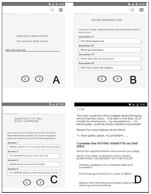
The respondent evaluates combinations of elements, not single elements alone. It is the set of 24 combinations, created according to an underlying experimental design, which is the mechanism by which the respondent’s underlying attitude towards a topic can be obtained and the tendency to be politically correct defeated or at least strongly stymied. The vignette, appearing as an example in Figure 1, presents a combination of elements in a manner which seems haphazard, almost created by random.

FIG 1

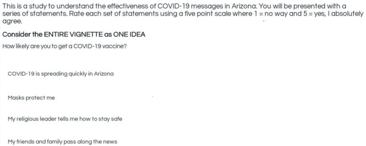
Figure 1: Example of a vignette.

The reality underlying the construction of the vignette is as far away from randomness as one can get with a systematic design. It is true that the combination is not written to tell a story. The objective of the vignette specifically, and Mind Genomics generally, is, figuratively, to ‘throw combinations of messages at the respondent, and see the rating.’ There is no underlying store to which the respondent can anchor, and be consistent within that anchor, and common principle. Rather, Mind Genomics is simply the response to seemingly random combinations. The respondent sits at the computer for about two-minutes, responding to 24 of these combinations, feeling that they are random, not realizing that the combinations have been systematically created. The respondent attempts to cope with the overload, but quickly relaxes into an almost automatic response, the type called System 1 by Nobel Laureate, Daniel Kahneman [11]. The respondent eventually ends up assigning the rating in an almost automatic, passive way, frustrated in the attempt to ‘game the system’ by the rapidly appearing and disappearing combinations.

There are two powerful aspects of the experimental designs used by Mind Genomics, of which the 4×4 (four questions, four answers to each question) is only an example. The first aspect is that the elements are statistically independent, viz. in a statistical sense all 16 elements are independent so that they can be used without concern in an OLS (ordinary least-squares) regression to uncover the relation between the elements and either the response or the linkage of the element to response time, the time needed to process the information and respond. The second aspect is that all the 24 vignettes used by a respondent are different from the 24 vignettes evaluated by a second response. The benefit there is that the Mind Genomics procedure covers a lot of the design space [12].

Across the set of 24 vignettes each person will encounter the same number of each of 11 different structures, albeit with different specific elements. The structure is defined as the questions which generate the elements, but not the specific elements themselves. The 11 structures comprise the six different structures for two-element vignettes, (AB AC AD BC BD CD), the four different structures for three-elements vignettes (ABC ABD ACD BCD), and the one structure of four elements (ABCD). We will see that some of these structures are, on average, stronger performers than other structures, when the data from the respondents is analyzed by structure.

Step 4: Run the Experiment and Create a Simple Topline Report (Surface Analysis)

Mind Genomics studies are run entirely on the internet, in a structure which is presented as a survey, not as an experiment. The appellation ‘experiment’ often irritates and confounds prospective respondents. The 500 respondents were members of a set of panels, used by the online study vendor, Luc.id of Louisiana. Luc.id provides populations of respondents from different geographical areas, of specific demography and activities. The panelists had to be residents of Arizona over the age of 18.

Table 2 shows the average ratings on the 5-point scale, and the average response time for each of the 11 structures. Each vignette in the study was assigned one of the 11 structures, depending upon the elements appearing, those elements dictated by the underlying experimental design. The respondent rated each vignette with the rating and the response time recorded. The response is operationally defined as the number of seconds, to the nearest tenth of second, elapsing between the appearance of the vignette and the rating.

Table 2: How average rating and average response time covary with structure of the vignette

Structure Questions

Rating

Response Time

ALL Total

3.4

3.8

AD Risk News

3.4

4.0

AB Risk Masking

3.4

4.0

ABC Risk Masking Trust

3.4

3.9

CD Trust News

3.5

3.8

BCD Masking Trust News

3.4

3.8

ACD Risk Trust News

3.4

3.8

ABCD Risk Masking Trust News

3.4

3.8

ABD Risk Masking News

3.4

3.8

AC Risk Trust

3.1

3.8

BC Masking Trust

3.4

3.7

BD Masking News

3.5

3.6

Table 2 shows a modest range in the average ratings, from a high of 3.5 to a low of 3.1). This suggests that the either the elements are seen to be equal, or there are deep differences among people in the types of elements with which they agree, but these deep differences cannot easily be seen. The differences are not emerging out the structure of the vignette, suggesting that respondents ‘graze’ for the information they need, rather than proceeding linearly through the vignette. If respondents were to proceed linearly through the text of a vignette, the vignettes with more elements would show higher response times, due to the longer times needed to read three and four elements. In contrast, the vignettes with fewer elements would show lower responses times but they do not. The data suggest that it is the nature of the information which drives the response times. The topic of ‘risk’ is the most engaging, the topic of ‘masking’ the least engaging.

One of the recurring themes in social research is that the differences in the responses may well be due to who the respondent IS. That is, there is an ongoing belief that people vote based upon who they are. Thus, much of the news reported focuses on differences between groups of people who can be easily identified, such as gender, or age-cohorts (e.g., Baby Boomers vs. Millennials vs. Generation X, etc.).

The data from this study allows us to look at the average rating and the response time from different, identifiable groups, as shown in Table 3. Table 3 shows the average age, the average rating, and the average response time, for each defined group. Table 3 also shows averages from transformed data (see Step 5 below). We see little difference in the average ratings, but we do see substantial differences in the average values of the response times, differences which make sense. Young respondents (age 18 – 29) read and rate much faster than average (2.8 seconds per vignette vs. 3.8 seconds on average), whereas old respondents (age 65+) read and rate more slowly (5.5 seconds on average).

Table 3: Average age, 5-point rating, response time (RT), and binary transformed ratings) for Total, Gender and Age, respectively

table 3

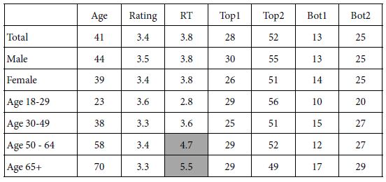
It is important to keep in mind that the differences in response time may be due both to age and to topic. We know that when the topic moves from social issues such as vaccine and COVID-19, to issues that are more ‘fun’ such as products, the response time usually diminishes, perhaps because the respondent does not have to think about the topic quite as seriously.

Step 5 – Prepare the Data for Regression Linking Elements to Responses

The underlying experimental design allows us to link the presence or absence of each element to the rating and to the response time. Yet, there is a problem with the data, one which must be solved before the analysis can proceed in a smooth manner. The problem or issue is the way one should interpret the results of a Likert Scale. From author HRM’s experience, managers commissioning the study or working with the data often ask about the meaning of the rating, such as ‘what does a 4 mean on the scale, from a practical point of view?” What the manager needs is a more black-and-white metric, one which reduces the task of interpreting the data.

Consumer researchers and public opinion pollsters are well-aware of the problems with managers interpreting the data for simple scales. Indeed, in the words of S.S. Stevens, Doyen of modern-day psychophysics, ‘one of the hardest problems in science is to go from a scale to a yes/no’ [13].

Researchers world-wide have suggested simple ways of dividing Likert Scales. For the five-point scale used today, researchers had suggested using the ratings of 5 & 4 as the key variable. Vignettes rated 5 or 4 are assigned the value of 100, vignettes rated 1, 2 or 3 are assigned the rating of 0. This is called the ‘Top2 Box,’ abbreviated here ‘Top2’. The reason is simple; The top 2 scale points (or ‘boxes’) are the ones selected.

In this spirit, we have created four new variables to use in our exploration:

Agree with the need for/goal of vaccination

Top1: Rating of 5 transformed to 100, ratings of 1, 2, 3 and 4 transformed to 0

Top 2: Rating of 5 and 4 transformed to 100, ratings of 1, 2, and 3 transformed to 0

Bot1: Rating of 1 transformed to 100, ratings of 2, 3, 4 and 5 transformed to 0

Bot 2: Rating of 1 and 2 transformed to 100, ratings of 3, 4 and 5 transformed to 0

A small random number less than 10-5 is added to each of these numbers to create some variability around the ratings. When a respondent assigns all ratings 1 & 2, or 4 & 5, respectively, regression analysis will ‘crash’ because the regression needs a bit of variation in the dependent variable, the transformed number. The transformation prevents the crash of the regression modeling but is far too small to affect the data in a meaningful way.

Step 6: Relate Elements to Ratings by OLS Regression

OLS (ordinary least-squares) regression relates the presence or absence of the 16 elements to the dependent variable. We begin with two dependent variables, the 5-point rating scale, and the response time. We add four more dependent variables, emerging from our transformation to the binary scales; Top1, Top2, Bot1, Bot2. These were defined in Step 5.

The basic equation is simple:

Dependent Variable = k0 + k1 (A1) + k2(A2) … k16(D4)

Simply stated, the dependent variable is the sum of a single base number (additive constant), and the contributions of the elements in the vignettes, these contributions being estimated by the OLS regression, and shown as k1-k16.

The value k0 is not estimated for the response time, RT, simply because it has no meaning. The value k0 is also not estimated for the 5-point scale, to give a sense of the number of rating points contributed by each element. For the other five dependent variables, k0 is the estimated value of the dependent variable in the case where all the elements in the vignette are 0, viz., absent. Such a situation, a vignette without elements, is impossible according to the underlying experimental design.

Table 4 presents the data from the Total Panel, showing only the positive coefficients. The data are incomplete, but to show all coefficients, negative values as well as 0, overwhelms the reader. The positive coefficients are those which drive the response towards the top of the scale, whether the scale be Top1 (highest possible agreement with getting a vaccine), Top2 (strong agreement with getting a vaccine), or towards the bottom of the scale, Bot1 (highest possible disagreement with getting a vaccine), or Bot2 (strong disagreement with getting a vaccine).

Table 4: How the 16 elements drive the ratings, both transformed binary ratings, original 5-point rating, and response time.


TOP1 TOP2 BOT1 BOT2 RATING

RT

Additive constant

28

53 15 28 NA

 NA

A1 COVID-19 is spreading quickly in Arizona 1.0

1.1

A2 New strains of the virus – causing concern 0.9

1.1

A3 Government should be doing more 0.9

1.0

A4 Everyone should take care of themselves

1

1.0

1.1

B1 Stay home so I don’t have to worry about masks 1 1.1

1.2

B2 Masks protect me 1.0

1.1

B3 I mask up to protect older people that I love 1 1.0

1.2

B4 Avoid places where people aren’t wearing masks 1.0

1.2

C1 I trust my doctor’s advice 1.0

1.1

C2 My employer gives the best information about the virus 1.0

1.1

C3 My religious leader tells me how to stay safe 1.0

1.1

C4 I listen to my family and children about staying safe

1

1 1.1

1.1

D1 Local Arizona media keeps me up to date 1.0

1.0

D2 Social media gives me the fastest news 1 1.0

1.0

D3 News from my employer is accurate 1 0.9

1.0

D4 My friends and family pass along the news 1 1.0 1.0

The actual interpretation of the data is left to the reader, but the Total Panel shows little in the way of patterns. The additive constant for Top1 tells us that about a quarter of the responses would be ‘5’ in the absence of the elements. Note that the additive is a theoretical, computed value, since all vignettes comprised 2-4 elements. The additive constant is a good parameter to give a sense of the ‘baseline’ level of feeling. For Top1 (strongest interest), we see an additive constant of 28, low, and in need of a ‘push’ from the elements. When we look at positive responses, 4 and 5, combined into the variable Top2, see a little over half, 53% of the responses are expected to be positive. Similarly, when we look at the negative part of the scale, about 15% of the responses are expected to be extremely negative, and a little less than twice that number (viz., 28%) are expected to be strongly or moderately negative.

Our next task is to use judgment to identify, where possible, elements with high positive coefficients for either Top1 (ideal) or Top2 (strong or moderate interest in the vaccine). Table 4 shows us no strong elements at all, a disappointing finding. From our first effort, and looking at the total panel, we find that no elements drive interest in being vaccinated. The answer may be either that we have not found that ‘magic bullet,’ or that we may have a powerful element, but it is lost in ‘noise’. We soon will see that the latter is probably the case, that there is noise in the data emerging from different groups of people, with varying, occasionally conflicting opinions.

A second look is at the response times. Do opinions of these messages engage the respondent? Engagement might be either good or bad, good when the message is a driver for vaccination, bad when the message is irrelevant, and a time waster. The model for the response time is lacking a constant. No elements engage by having the respondent focus on the element for more than 1.2 seconds.

Our first conclusion is that there is no pattern, that all the messages are irrelevant, and that the experiment was unable to uncover any element which is promising. That is, when we treat all of the respondents in the same way. We are either dealing with irrelevant elements, certainly a strong possibility in the absence of any other reasons to think otherwise, OR we are dealing with elements which push in opposite directions, cancelling each other out.

Step 7: Granular Understanding by Clustering to Uncover Mind-sets

We saw above that there are few differences among the elements in terms of those driving positive interest to get vaccinated. Some of this ‘flatness’ may emerge from the fact that people think in different ways, effectively canceling each other when they are blended together in a database which does not recognize these individual patterns.

Mind Genomics studies have uncovered the existence of different groups of ideas which go together, different mind-sets of these related ideas. It is not that people differ, but rather that the ideas they hold are of different types, even when the topic is the same. By clustering the patterns of coefficients across the individual respondents, viz., putting together people with similar patterns, Mind Genomics can identify these basically different groups of ideas. These different groups are the so-called ‘mind-sets’ [14,15].

The process of clustering is a standard statistical method. The method of k-means clustering looks at the 16 coefficients of each respondent, based upon the relation between Top2 (dependent variable) and the presence/absence of the elements. The additive constant is computed, but not used here. The clustering, based upon similarity of patterns, divides the 500 patterns into one, two, and the three groups. Each respondent is a member of only one of the groups, with two groups, or a member of one group when three groups are extracted [15].

The original analysis by clustering uses the coefficients obtained for the Top2 analysis, meaning that ratings of 4 and 5 are converted to 100, and ratings of 1-3 are converted to 0. We will remain with that clustering. For the prescription of what to feature in the messages, we will the make analysis more stringent, however. We will look at the models or equations relating the presence/absence of the 16 elements to rating 5:, How likely are you to get a COVID-19 vaccine? 1=No way 5=Yes, I absolutely agree. This is the Top1 equation, showing which elements are the strongest. Thus, we keep the clustering method the same (based on Top2), but the reportage as more stringent (use Top1 data for modeling).

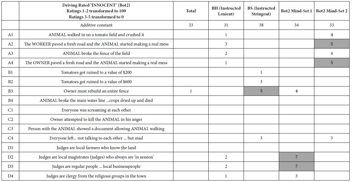
Table 5 shows the positive coefficients for the Top1 model. It is clear that there are few elements which are strongly effective for each mind-set. These are the elements to select for the final messaging. The selection is far easier when the criterion is low, but the downside of the process is that the coefficients are low, albeit the most powerful. The only exception to the pattern of low coefficients emerges from mind-set MS3, the Pandemic Activist, comprising about 1/3 of the respondents.

Table 5: Strongest performing elements for vaccination, viz., highest coefficients for TOP1 (Definitely will vax)

table 5

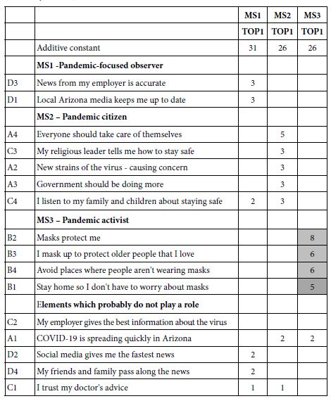
The important consideration here is that the message be strong. Choosing a message which contributes to rating 5 (definitely will vax) is better than a message which contributes to both rating 4 and 5 (definitely/probably will vax.) The choice towards the messages which are most effective, recognizing that there can probably be at most three messages.

The final thing to keep is mind is the radically different elements which score well. These elements are clearly touching different aspects of the COVID-19 experience, suggesting quite different mind-sets among the respondents.

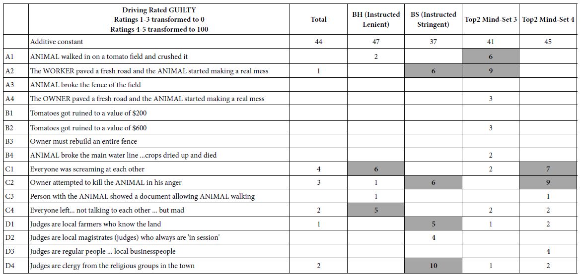
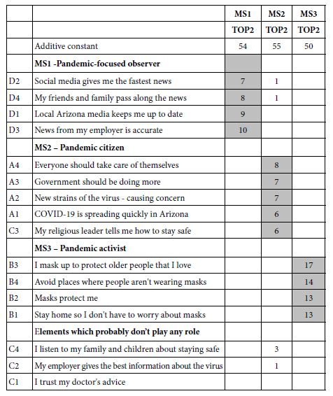
To get a sense of the power of a tough criterion, such as Top1, consider the same Table, but the more typical case, wherein the elements are the strong performers, but for Top2 (Definitely/Probably be vaccinated). Many of the elements are the same, but the first impression from Table 6 is a greater richness of information. That richness is certainly satisfying, but when it comes time to put the information into practice one will inevitable be confronted with the question about which of the strong performing elements is actually the ‘strongest’. That is, having a wealth of information is rewarding for the stage when one seeks understanding, but problematic when the task is to choose the one, two, or three elements from the set, and allowed only those choices.

Table 6: Strong performing elements for vaccination, viz., highest coefficients for TOP2 (Definitely will vax, probably will vax, ratings 5 and 4)

table 6

Step 8: Understand the Engagement Power of the Elements Using RT (Response Time)

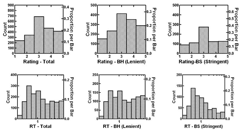
Figure 2 shows the distribution of measured response times for the vignettes, independent of the structure of the vignette and the specific elements. A great many vignettes are rated faster than two seconds, most vignettes rated in fewer than five seconds. As we see below, there is very little difference in the response times linked to the different messages.

fig 2

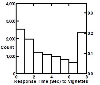
Figure 2: Distribution of measured response times for the vignettes.

The final element-level analysis links the elements to estimated response times for the elements. The equation for response time comprises the 16 independent variables, the elements, but does not make provision for an additive constant. The rationale for leaving out the additive constant is that in the absence of any elements (again a hypothetical case) there is no expectation of any response at all.

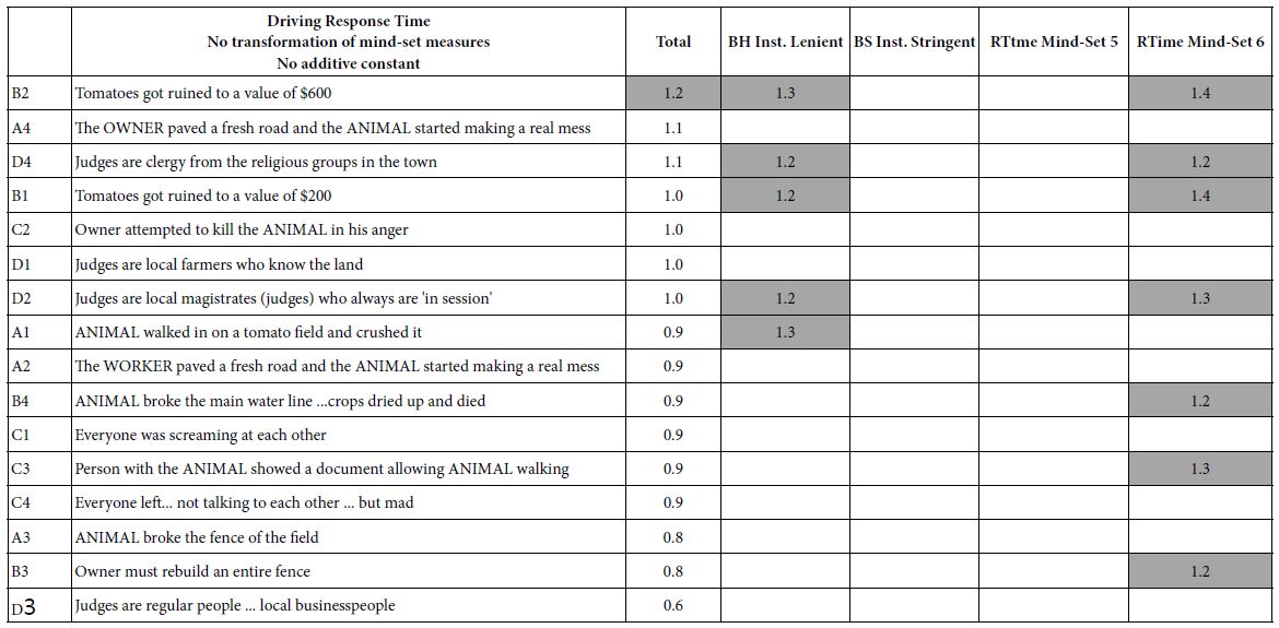
Table 7 shows the estimated response time attributed to each element. The important thing to note is that strong performing elements in Table 5 are not necessarily those with long response times, viz., those which are engaging. Indeed, most of the response times are around 1.0 – 1.2 seconds per element, with a few shorter and a few longer. The results suggest that the respondents do not ‘whiz through’ the elements when making their ratings. They do ‘whiz through’ for other studies, especially the less serious studies having to do with brands and products. Thus, one can feel good that the respondents are actually paying attention to the information, at least in terms of taking the time to read the vignettes.

Table 7: Estimated response time for each element, by each mind-set.

table 7

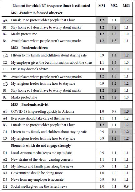
Step 9: Artistic Judgment for Next Steps – Identify the Elements Which have the Greatest Staying Power

One of the ongoing issues in any messaging campaign is the probability that at some time the messages will simply ‘wear out.’ The wear out is habituation, a well-known phenomenon in psychology, wherein the stimulus fails to evoke attention as it continues to be repeated. Experimental psychology demonstrates this phenomenon in rigorous studies, such as the measuring attention reactions of cats presented with the same tone in a steady, expected, repeated, monotonous fashion. Habituation occurs in our everyday life; simply witness people who live near train tracks, and who quickly become accustomed to the noise.

How can we identify messages which have staying power, especially messages which are good to being with? One way to do this uses the actual data from the study. This time, however, the data matrix is divided into equal fourths (viz., vignettes 1-6, 7-12, 13-18, and 19-24). One takes the set of elements to be used in the proposed messaging, viz. one winning element for each mind-set. The selection of the winning element is a matter of judgment, and may involve ‘gut feelings,’ viz., intuition, which move beyond the actual data. The approach here considered only the elements doing well among the three vignettes in the Top1 metric. These were D1, A2, B4:

Local Arizona media keeps me up to date

New strains of the virus causing concern

I mask up to protect older people that I love

These three elements became the only predictors of Top1, Bot1, and RT (response time). The vignettes (fourth = 2, fourth = 3), and for the final vignettes (fourth = 4). By looking at the coefficients for each element across the four sets of evaluations, we get a sense as to whether or not the elements are ‘wearing out’.

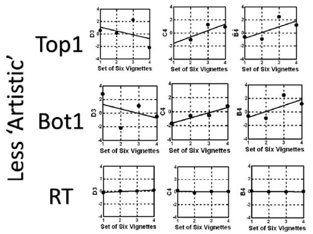
Figure 3 suggests that repeating the messages will enhance the impact of each element in terms of driving the respond to agree to a vaccine (Top1), and for the most part will reduce the resistance (Bot1). The only exception to this general trend is element B3, which shows no loss in negativity with repetition, and perhaps even a slight increase, perhaps resentment at being reminded. The same analysis can be done for any set of messages, to determine whether the messages will change with repeated exposure. Figure 4 show the same analysis, this time for strong performing elements using their coefficients for Top1, but a combination ‘artistically’ sensed as inferior:

fig 3

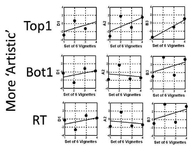
Figure 3: Likely wear-out of messages for the vignette which seems ‘more artistic’. The graphs show the expected change of the coefficient for each promising element, when evaluated in sets of six vignettes each. The combination comprises D1, A2 and B3, winning elements from the three mind-sets, selected by artistic sensibility as ‘working together’.

fig 4

Figure 4: Likely wear-out of messages for the vignette which seems ‘less artistic’. The graphs show the expected change of the coefficient for each promising element, when evaluated in sets of six vignettes each. The combination comprises D1, A2 and B3, winning elements from the three mind-sets, selected by artistic sensibility as ‘working together’.

News from my employer is accurate

I listen to my family and children about staying safe

Avoid places where people aren’t wearing masks

The approach does not replicate the actual events in the world, but rather may be analogous to the process of ‘accelerated aging’ in the world of food science, with the attempt to determine the ‘shelf life’ of a product, so that the product can be pulled from the market shelves before it changes in quality and becomes significantly less palatable [17].

Step 10: Find the Mind-sets in the Population for Targeted Messaging

Ongoing patterns of results from Mind Genomics cartographies, of the type done here, albeit in many other areas, suggest that there exist clearly different mind-sets, but that these mind-sets are distributed in the population in an almost random way, at least to the outside researcher who only has data from who the respondent IS (geo-demographics), how the respondent THINKS (personas based upon large-scale segmentation), or how the person BEHAVES (either in everyday life, or in tracked shopping behavior.)

In none of the standard analysis of WHO, THINKS, or BEHAVES can we find easy covariation with the mind-sets. That is, it is quite unlikely to know how a person will think about a topic just be knowing the typical information available to the researcher. There may on occasion be some happenstance covariation that can be used, but as far as a robust system to link together mind-sets and people, there does not seem to be a recognized tool.

Table 8 shows the distribution of the three mind-sets by gender, by age, and by ethnicity. It is clear from Table 8 that simply finding the mind-set will be difficult in the population. The next best thing is to use set of messages woven together to incorporate the essence of one message for each mind-set, as Figure 3 suggests.

Table 8: The distribution of respondents by mind-set, gender, age, and ethnicity. The numbers in the body of the table are the actual number of respondents who classified themselves at the start of the Mind Genomics experiment, in the self-profiling questionnaire


Total

MS1 MS2

MS3

Total

494

181 169

144

Male

192

65 62

65

Female

302

116 107

79

Age 18-29

160

62 51

47

Age 30-49

181

63 60

58

Age 50-64

79

30 28

21

Age 65+

74

26 30

18

Caucasian

322

120 118

84

Latinx

85

30 27

28

Other

81

30 21

30

The fact that mind-sets can so easily emerge from data, and be found at any level of granularity desired, and virtually for any topic, in as a fast as one hour, suggests that a new way of thinking is needed to use the mind-set segments. It is no longer sufficient to spend days, weeks, or months cogitating over the application of mind-set segmentation when the actual results had been obtained in a matter of hours.

During the past four years authors Gere and Moskowitz have worked on algorithms to classify the respondent as a member of a mind-set, recognizing that the algorithm should be quick to develop, easy to implement, and inexpensive. The algorithm also must minimize the ability of a respondent to ‘game the system,’ by guessing what the interviewer wants to hear.

The approach developed emerges out of the actual experiment and data set used to create the mind-sets in the first place. This first step ensures that the elements used to assign a new person to a mind-set are relevant to the topic, moving away from the potential error-propagating step of searching for other language that can be used for assigning the respondent to the mind-set. This first is close in, and immediate. As soon as the mind-sets are determined so is the performance of each element for each mind-set.

The second step uses a Monte Carlo system to introduce noise, and then assign respondents to the mind-set in the present of the noise.

The third step aggregates the data and generates the decision rule which is most resistive to the introduced ‘noise’ and correctly types of the mind-sets in the presence of the noise.

The resulting approach is called the PVI, the personal viewpoint identifier. The set-up is done according to a Microsoft Excel template (Table 9). The template requires the researcher to provide specific information about the mind-sets (viz., name, feedback), as well as an optional video or landing page corresponding to the mind-set, right after the respondent is assigned to one of the mind-sets. At the bottom of Table 9 is the summary data from the mind-sets, used by the PVI to create the actual calculation table.

Table 9: Template for the creation of the PVI (personal viewpoint identifier).

table 9

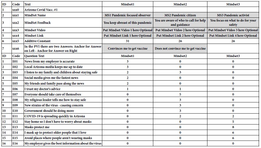
Once the input in Table 9 has been processed to create the PVI, the result comes back in a link. The respondent who clicks on the link is led to the PVI on the web. Figure 5 shows the introductory page, which introduces the respondent to the reason for the short study, obtains permission, and obtains background data. Figure 6 shows the set of questions, comprising background questions (not part of the classification algorithm), and six questions answered by one of two answers. These six questions are the PVI. Each respondent sees the six questions in a different order. The data are stored in a database for further work, and the results sent back to the respondent either in a detailed form, or just an email with mind-set membership, and something about the mind-set to which the respondent belongs (Figure 7).

fig 6

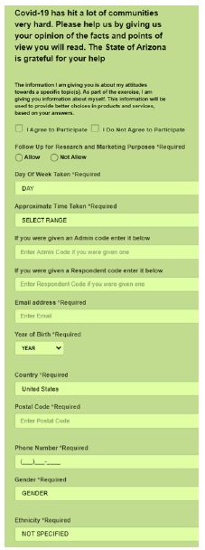
Figure 5: The orientation page for the PVI. The link (as of January, 2021) is: https://www.pvi360.com/TypingToolPage.aspx?projectid=1270&userid=2

fig 6, 6

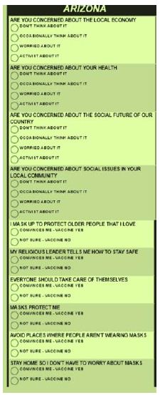
Figure 6: The questions about one’s concerns, and the six questions for the PVI.

fig 7

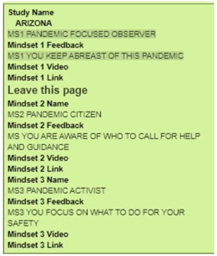
Figure 7: Feedback page for insertion into the database. The respondent receives a simple email showing the three mind-sets, viz., their names and the feedback, as well as the mind-set to which the respondent belongs. This example is from a person in Mind-Set 1, the Pandemic Observer.

Discussion and Conclusions

The study reported here typifies what, in the emerging science of Mind Genomics, is called cartography, for want of a better word. The cartography is not designed to test hypotheses, in the traditional view of some scientists [18]. There are no working hypotheses to falsify. The cartography, as the word connotes, explores the topic, and maps its detailed features. Here the features are the words. As we begin to create cartographies, there are usually several sequential cartographies or iterations. At the start we need not know whether the questions are the correct ones, and certainly whether the answers are correct or event relevant. Yet, we do the experiment, we put a ‘stake in the ground,’ discover what works and embellish it, discard what does not work, and then add new material for the next iteration [19].

Although this might not seem to be the most elegant way of creating a database, it certainly is the quickest, and in fact allows the database to create to be created by all sorts of people, whether these are professionals in the healthcare world, patients, doctors, or hospital administrators, or even relatives of those who are patients. The notion is not to get it right, because there is no ‘right’ – at least not at the start. Rather, the notion is that through responses to descriptions, the vignettes, the underlying patterns will emerge, in the way the underlying structure emerges from the many pictures taken by the MRI and reassemble the structure after the fact through a computer program.

A key benefit of Mind Genomics is its availability to anyone, expert or amateur alike, and the possibility that the discoveries may be made by virtually anyone. A dedicated analyst working with dozens of transcripts of interviews lasting an hour or two about the topic might emerge with similar findings, but not as crisp, nor as data rich. In contrast, the novice but avid researcher, can do an iteration overnight, following the templated approach of Mind Genomics. The templated approach forces the research to focus on the messages, do the experiment, obtain the data, and face the bare facts, specifically how the messages drive the response. The data are archival, the learning is incremental and expansive, and the result resides in a searchable data warehouse, ready for reanalysis to provide new insights. The information can be searched for words, for meanings, and for new correlations, done, at virtually any time after the study, and by virtually anyone. These data from the first study on COVID-19 in Arizona give a sense of the potential.

Practical Conclusions – Driving Vaccination in Arizona

The focus of this paper is both on method and on results. Both are important during this period of the COVID-19 pandemic. The rationale of showing what can be done in one day is not so much to provide a perfect answer or write a perfect paper, as it is to show a revolutionary change in what could be learned in a short time at a low cost. Cost, time, and the power to iterate to a better answer are important for the obvious reasons; costs of medical treatment and of medicines are increasing, making prevention increasing attractive. The more that we can learn about people ‘in the moment’ with respect to issues which emerge, the more likely it will be that we can communicate more effectively with people. This communication includes providing the necessary information and the suggestions, both tailored to the mind-set of the person, and perhaps both more convincing, more motivating. It is no simple thing to motivate people. The faster and easier it becomes to learn the necessary facts and words, ideally in ‘real time,’ the more likely it we be that people will be guided gently, through words, to live healthier lives, and to take better care of themselves. The cost of the medical interventions might be lower.

The data here suggest that it is vital to consider the different mind-sets of respondents. In light of the speed, ease of analysis, and low cost, as well as a tool to determine the mind-set of the respondent, the prudent action would be to do one to three or four Mind Genomics cartographies, as done here, eliminating the poor performing elements, and building upon the elements which look like they work. Table 6 shows the dramatic increase in performance of elements, and the clearly different mind-sets. Several more cartographies, each last no more than a day, should build a new set of ‘Table 6’s’ with increasingly strong performing elements. It is unlikely that there is a single ‘magic bullet,’ for all mind-sets, but there are clearly a number of strong elements for each mind-set.

Acknowledgments

Attila Gere thanks the support of Premium Postdoctoral Research Program of the Hungarian Academy of Sciences.

References

  1. Benyamini Y (2011) Why does self-rated health predict mortality? An update on current knowledge and a research agenda for psychologists. Psychology & Health 26: 1407-1413. [crossref]
  2. Benyamini Y, Blumstein T, Lusky A, Modan B (2003) Gender differences in the self-rated health–mortality association: Is it poor self-rated health that predicts mortality or excellent self-rated health that predicts survival? The Gerontologist 43: 396-405.
  3. Dulmen S, Sluijs E, Dijk L, Ridder D, Heerdink R, Bensing J (2007) Patient adherence to medical treatment: a review of reviews. BMC Health Services Research 7: 55. [crossref]
  4. Boodoosingh R, Olayemi LO and Sam FAL (2020) COVID-19 vaccines: Getting Anti-vaxxers involved in the discussion. World Development, 136: 105177. [crossref]
  5. Burki, T (2020) The online anti-vaccine movement in the age of COVID-19. The Lancet Digital Health 2: 504-505. [crossref]
  6. Kennedy AM, Brown CJ, Gust DA (2005) Public Health Reports 120: 252-258. [crossref]
  7. Zimet GD, Rosberger Z, Fisher WA, Perez S, Stupiansky NW (2013) Beliefs, behaviors and HPV vaccine: correcting the myths and the misinformation. Preventive Medicine 57: 414-418. [crossref]
  8. Gere A, Zemel R, Papajorgji P, Moskowitz H (2019) “Candy Is dandy”: The mind of sexuality as suggested by a Mind Genomics experiment. In Sex, Smoke, and Spirits: The Role of Chemistry, 17-31.
  9. Sullivan, GM, Artino Jr AR (2013) Analyzing and interpreting data from Likert-type scales. Journal of Graduate Medical Education 5: 541-542. [crossref]
  10. Bellissimo, N, Gabay, G, Gere, A, Kucab, M and Moskowitz, H (2020) Containing COVID-19 by Matching Messages on Social Distancing to Emergent Mindsets: the Case of North America. Int J Environ Res Public Health 17(21): 8096 [crossref].
  11. Kahneman D (2011) Thinking, Fast and Slow. Macmillan.
  12. Gofman A, Moskowitz H (2010) Isomorphic permuted experimental designs and their application in conjoint analysis. Journal of Sensory Studies 25: 127-145.
  13. Stevens, personal communication to Howard Moskowitz, 1968.
  14. Moskowitz HR (2012) ‘Mind Genomics’: The experimental, inductive science of the ordinary, and its application to aspects of food and feeding. Physiology & Behavior 107, 606-613. [crossref]
  15. Moskowitz HR, Gofman A, Beckley J, Ashman H (2006). Founding a new science: Mind Genomics. Journal of Sensory Studies 21: 266-307.
  16. Jain AK, Dubes RC (1988) Algorithms for Clustering Data. Prentice-Hall, Inc.
  17. Schwarz M, Rodríguez MC, Sánchez M, Guillén DA, Barroso CG (2014) Development of an accelerated aging method for Brandy. LWT-Food Science and Technology 59: 108-114.
  18. Popper KR (1963) Science as falsification. Conjectures and Refutations 1: 33-39.
  19. Benyamini Y, Idler EL, Leventhal H, Leventhal EA (2000). Positive affect and function as influences on self-assessments of health expanding our view beyond illness and disability. The Journals of Gerontology Series B: Psychological Sciences and Social Sciences, 55(2), P107-P116. [crossref]
fig 2

Development and Testing: Cervical Cancer Prevention Questionnaire Based on Theory of Planned Behavior in Chile

DOI: 10.31038/AWHC.2021411

Abstract

The purpose of this study was to developmentally and psychometrically validate the cervical cancer prevention questionnaire (CPCC-16) based on Theory of Planned Behavior in Chilean women. The patient sample was 967 women. Confirmatory factor analysis was used to evaluate factor structure, Cronbach’s alpha for internal consistency and t-test for criteria validity. The development and validation of the questionnaire resulted in six factors with 16 items, demonstrating a bi-factorial structure. Cronbach’s alpha was higher than 80 in the questionnaire and its factors. To generate a valid and reliable questionnaire that measures, under a theory of behavior, more than one preventive behavior in cervical cancer is an important advancement that fills a gap in nursing research.

Keywords

Cervical cancer, Prevention, Instrument development

Precis: The CPCC-16 questionnaire is a validated and reliable instrument, with 16 items distributed in a bi-factorial structure, useful for clinical and research area.

Call Outs: Behaviors are the principal causes of deaths from cancer, and thus, a reliable and validated questionnaire is necessary to measure these behaviors (before method).

The validated and reliable questionnaire will be useful to measure cervical cancer preventive behaviors as a whole, but it will also be useful to identify theory constructs (after method).

The new questionnaire will be useful to measure more than one preventive behavior in cervical cancer; therefore, it fills a gap in clinical and research area (after discussion).

Introduction

Theory of Planned Behavior (TPB) has been a framework to explain and predict behaviors [1], and its ability as a framework intervention has been supported by previous studies [2-4]. TPB postulates that the motivations of people to change are based on their perceptions of norms, attitudes, and control over behaviors, and each of these factors can either increase or decrease the intention to change their behavior. The intention to change behavior is directly related to behavioral change [5,6]. Cervical Cancer (CC) prevention has been one topic that has been studied under this theory [7-11].

There are two methods to stop CC: to prevent its pre-cancer and to identify and treat the cancer before it becomes a true cancer [12,13]. The first method includes behaviors, including the use of condoms during sex, limiting the number of sexual partners, not smoking and obtaining the Human Papilloma Virus (HPV) vaccine; the second method includes having regular screenings [13,14]. The CC prevention questionnaire (CPCC-16) was developed based on TPB to measure CC preventative behaviors.

Background

Even where screening is widely available and methods to prevent CC are known, there is an important barrier in adopting these methods by women. Thus, understanding the factors that affect preventive behavior remains an important issue.

TPB has been previously used by several studies to understand how cervical cancer preventive behaviors are carried out, and the intent to perform the behavior is explained [8,15,16]. The main behaviors studied are those related to the detection of CC, such as adherence to the HPV [8,11,17] tests [7,10,15,18,19]. Some studies have described the use of TBP and HPV vaccination intentions [16,20]. The use of condoms has been studied; however, these studies are not always related to CC prevention and are mainly examined in an adolescent population [21,22]. To the best of our knowledge, there have been no previous studies using questionnaires to measure more than one preventive behavior using TPB as a framework.

Regarding the psychometric properties of the questionnaires used in CC prevention, the reliability and/or validity of the instruments has not always been reported [10,11,16,20,21], or they have been incompletely reported [7-9,17,19]. Research on TPB with other behaviors indicates the same problem [2,3,23]. The author and creator of TPB [1] supports these findings, describing the measures of the theory constructs as fallible with respect to reliability and construct validity, and thus, it is difficult to test the theory.

With regard to TBP as a framework, the literature indicates that the most important theory construct studied has been intention [24] and that some research studies have only partially studied the TBP components [15].

Behaviors are the principal causes of deaths from cancer, and infections such as HPV are responsible for up to 25% of cancer cases in low and middle-income countries [25]. If the solid foundation of TBP and the relevance to prevent CC worldwide are considered, then a questionnaire that is reliable and valid, which permits the ability to simultaneously measure more than one CC preventive behavior and to test the four-principal construct of TPB, may be useful in different countries and contexts. Thus, it is useful to have a CC prevention questionnaire based on TBP.

The purpose of this study was to develop and psychometrically validate a new questionnaire based on Theory Planned Behavior (TPB) with relation to Cervical Cancer (CC) prevention (known as the CPCC-16 questionnaire).

Method

This study is a part of a larger cross-sectional study about Social Determinants related to the adherence to CC screening (FONDECYT #11130626); this article focuses on the development and testing of one of the questionnaires used in the project, which was performed in two phases: scale development and psychometric evaluation.

Sample/Participants

This research study was performed on a total of 967 Chilean females, between 25 to 64 years old, under Chilean national public health care coverage (known as FONASA); these participants attended four primary health care centers in the Servicio de Salud Metropolitano Sur-Oriente (Southeast Metropolitan Public Health Service) in Santiago, Chile. The sample size was calculated according to the larger study aims considering an effect size of 0.1, power analysis of 80%, 15 latent variables and 40 observed, and a significance level of 95%. The sample was obtained according to the recommendations related to the questionnaire validation [26-28]. The exclusion criteria included having had a hysterectomy and CC disease. Females who had agreed to participate were randomly selected and recruited by telephone between March 2014 and October 2015.

Scale Development

The questionnaire was developed based on TPB and according to Icek Ajzen’s recommendations [29]. The first step was to define the behavior; therefore, four behaviors were included: annual gynecological check, updated Papanicolaou test (Pap), condom use on sexual relations and having a single partner (at the same time). Behaviors related to the HPV vaccine or HPV screenings were not considered because they are not available in the public health care system where the study was performed. Figure 1 shows the construct and preventive behaviors considered in the questionnaire. The second step was defining the population; females between 25 to 64 years old were selected because they are the target group for cervical cancer screening and prevention interventions in Chile. The third step was formulating items; they were developed to assess the major constructs of TPB for each preventive behavior selected in the first step: attitude, subjective norm, perceived behavioral control, and intention. The items were given feedback from content experts and then pilot tested on ten females from the target population. The questionnaire was developed in the Spanish language and back-translated for this article.

fig 1

Figure 1: Theory of Planned Behavior Constructs and Cervical Cancer Preventive Behaviors considered in the Original Questionnaire.

Psychometric Evaluation

Construct validity was performed by Confirmatory Factor Analysis (CFA), and reliability was assessed using ordinal Cronbach’s alpha. Three models were adjusted: one model with the four TBP constructs, the second with a bifactorial model considering the four TBP constructs and the four CC prevention behaviors, and the last model considered the four constructs from TBP; four behaviors but three of them were grouped in one factor. Diagonally Weighted Least Squares (DWLS) were used to estimate the models because the variables were measured using the four-point ordinal scale. The fit model was evaluated using normed chi-squared (chi-squared/degree of freedom) with two comparative fit indices: Comparative Fit Index (CFI) and Tucker-Lewis Index (TLI); Root Mean Square Error of Approximation (RMSEA) was used as parsimonious fit indices. We considered CFI and TLI values >0.95, with RMSEA <0.05 as good; CFI and TLI values between 0.90-0.95 and RMSEA between 0.05-0.08 were acceptable; and CFI and TLI values <0.90 or RMSEA >0.08 were unacceptable. The statistical significance of each item as it is related to the factor, as well as whether an item shared a common conceptual meaning with the factor, was also considered. The PAP test and gynecological check status were used as external criteria to validate the questionnaire. The scores of each factors of the questionnaire were calculated by regression method, using standardized variables and the factor scores between women with adherence to CC screening and without adherence or with annual gynecological check and without it were compared using t-Student test for independent samples. Data were analyzed using R Statistical Program and the lavaan package.

Instrument

The proposed instrument (Appendix 1) consisted of 16 items related to CC prevention behaviors, which were divided into 4 dimensions according to the TPB constructs: attitudes (4 items), subjective norms (4 items), perceived behaviors control (4 items), and intentions (4 items). Each item was evaluated using a Likert scale of four alternatives (strongly agree/very good=1 to strongly disagree/very bad=4). Such a scale is used to force directionality of a response (de Vellis, 200 [30]) in a population where culture (Hispanic) tends to avoid conflict, resulting in a frequent selection of neutral alternatives (Antshel, 2002 [31]).

Ethical Considerations

This study was approved by the University of the Principal Investigator and by the health care service to which the women belonged. Written informed consent was obtained by all of the participants. All of the questions that the women had about CC were answered after the interview.

Results

The mean age of the participants was 43.37 ± 10.77 years, with the mean educational level being 10.97 ± 3.4 years. The CC preventive behaviors of the women are shown in Table 1.

Table 1: Characteristics of the women (n=967).

Characteristic

Value

Annual Gynecological Check, n (%)

537 (55.5)

Pap test in the last three years, n (%)

740 (76.5)

Have a partner, n (%)

766 (79.2)

Number of partners, mean ± SD (range)

2.69 ± 2.73 (1 to 40)

Use of Condom, n (%)

Always

65 (6.7)
Almost always

85 (8.8)

Never always

102 (10.5)
Never

715 (73.2)

Three models were calculated to achieve the best fit with the data (Table 2). The first model considered the proposed questionnaire with four factors, but the goodness of fit was not good (TLI <0.9 and RMSEA=0.231); the modified indices suggested the inclusions of correlations between the items with similar wording; and the correlations between intention and subjective norms (r=0.863) and intention and perceived behaviors control (r=0.939) were too high.

Table 2: Fit Statistics for the three models calculated (n=967).

Factor Model

x2/df

CFI TLI

RMSEA (CI 95%)

Four Factor

52.75

0.909 0.888

0.231 (0.226-0.237)

Eight Factor (bifactorial)

1.77

0.999 0.998

0.028 (0.020-0.036)

Six Factor (bifactorial)

1.94

0.999 0.998

0.031 (0.024-0.038)

These results suggested the consideration of second-order models, which explain the high correlations between factors, but this approach did not resolve the problem related to the correlations between preventive behavioral items. Thus, a bifactorial model was tested as a plausible alternative; one side with four factors related to TPB and the other side with four factors related to CC preventive behaviors were considered; the four factors within each side were correlated but not between the sides. The second model showed a good fit but with two high correlations: one of the correlations between an annual gynecological check and single partner (r=0.839) and the other between an annual gynecological check and updated PAP test (r=0.98). Thus, the decision was to place the correlations together into one factor. This model good fits the data, thus indicating a bi-factor structure with six factors, four of which were the TPB components and the other two were CC preventive behaviors. The results of external criteria validly of the questionnaire are in Table 3.

Table 3: External criterion validity through comparison between groups for Papanicolaou test and Gynecological check.

Factor

Papanicolaou Test in the last three years

Anual Gynecological Check

Yes

No   Yes No  
Mean (SD) Mean (SD) P value (a) Mean (SD) Mean (SD)

P value (a)

1. Cervical cancer preventive behaviors

-0.06 (0.39)

-0.16 (0.41) <0.001 -0.05 (0.38) -0.12 (0.41)

0.004

2. Condom use as cervical cancer prevention

-0.03 (0.63)

-0.05 (0.63) 0.631 -0.03 (0.64) -0.04 (0.63)

0.876

3. Attitude to cervical cancer prevention

-0.00 (-35)

-0.05 (0.38) .045 -0.02 (0.35) -0.01 (0.36)

.738

4. Perceived norm

-0.01 (0.40)

-0.11.46 .002 -0.02 (0.42 -0.06 (0.42)

.152

5. Perceived behaviors control

-0.00 (0.43)

-0.29 (0.65) <0.001 .03 (0.39) -0.19 (0.60)

<0.001

6. Intention

-0.01 (0.26)

-0.11 (0.30) <0.001 -0.00 (0.25) -0.07 (0.30)

<0.001

(a) T-Student was used to compare group values.

The new questionnaire (Appendix 1) called CPCC-16 (Conductas Preventivas en Cáncer Cérvicouterino-16 items/ Preventive Behaviors on Cervical Cancer -16 items) consisted of 16 items, which were distributed into six factors. The complete standardized parameters of the bifactorial model are shown in Figure 2. According to the bifactorial structure, each item corresponds to two factors. A summary of the CPCC-16 bifactorial model with factors, number of items and Cronbach’s alpha are shown in Table 4.

fig 2

Figure 2: Complete Standardized Parameters for the Bifactor Model of CPCC-16 (n=967).

Table 4: Name of factor, items and Cronbach’s alpha (n=967).

Factor

No of items

Cronbach’s alpha

1. Cervical cancer preventive behaviors

12 items

0.95

2. Condom use as cervical cancer prevention

4 items

0.93

3. Attitude to cervical cancer prevention

4 items

0.81

4. Perceived norm

4 items

0.87

5. Perceived behaviors control

4 items

0.81

6. Intention

4 items

0.86

CPCC-16 Questionnaire

0.94

Discussion

The first considerations to note are how the structure of the original questionnaire, without varying the number of items, was shown throughout the analysis. The initial questionnaire was created considering the underpinning of TPB constructs, where four factors were proposed. However, a questionnaire where only the theory constructs are considered was unacceptable, and thus, it was necessary to include the behavioral dimensions. However, although the second tested model with eight factors has good fit, it should not be considered a final model because it has two dimensions highly correlated (Pap test and Gynecological check). Thus, the result was a model with six dimensions in which all of the factors loading were significant, although some of the factors exhibited values lower than 0.4.

The final questionnaire was very consistent with another underpinning construct, that was not considered from the beginning (CC preventive behaviors). This result allows us to extend its usefulness, not only to test the TPB but also to analyze and explain CC preventive behaviors using this theoretical model.

The criteria validity shows that the final questionnaire is useful to associate the TPB constructs with the behaviors. The women with different CC screening or gynecological check behaviors did not show differences in condom factor scores; explanations could be because the condom use is not associated with cervical cancer prevention [32,33], or because the use of condom could be overestimated in the sample since it is an expected social behavior.

There are many contexts where the new questionnaire could be useful and where the TBP has demonstrated its utility: to assess the acceptability of preventive behaviors as a whole among the target group of women currently engaged in preventive programs [8,11], to evaluate the evolution of the intention across time [8,17], to evaluate the strategies of cervical cancer prevention programs [8,11,20] and to determine the factors that influence the behaviors [7,9,10,15,18,20]. CC remains a relevant problem, particularly in underdeveloped countries and ethnic minorities in developed countries [10]. Thus, instruments related to the prevention of CC could be very useful in many contexts. Theoretically based models of behaviors are also useful and necessary for the development of effective interventions [2,9,16,34].

A second consideration, related to the results, is why three preventive behaviors proposed in the initial questionnaire were collapsed into 1 factor, CC preventive behaviors (annual gynecological check, updated PAP test and to have a single partner). The second model tested demonstrated that each of the four behaviors proposed as a factor, but the results suggested other structures. This finding could be explained by it being necessary to consider who participated in the behavior and who decided it Therefore, CC preventive behavior factor focuses on behaviors in which the decision is primarily or only related with females, and the condom use factor indicates a behavior in which consensus is required between a woman and her partner.

Other explanations to account for the second consideration and indirectly related to the previous consideration could be that the CC preventive factor included behaviors that are not clearly associated with sexual life, and thus, it is not necessary to have an active sexual life. This is in contrast to the second factor where having sexual intercourse is the principal focus. The association between HPV and CC is one of the strongest described [13], but the relationship between sexual behaviors and CC risk has not been previously recognized by the women [35]. The use of a condom as CC preventive behavior was described in only 5.6% of the women [32], and in a Chilean study [33], only 27.6% of the women described sexual intercourse as a risk factor of CC. Thus, these reasons could explain the way that the preventive behaviors were grouped.

Related to factor loading of the items, there are only two items (items 3D and 4D), which have values less than 0.3, that could indicate that both items may be explained by the condom use factor rather than the intention and perceived behavioral control factors. To the best of our knowledge, there are no studies in which the results fit into a bifactorial model for preventive behaviors and TBP. This may be due to the focus of the research study on only one behavior and not as a group. There are many diseases that can be prevented by practicing some behavior, and the TPB is a solid theory that can help with its understanding. Thus, the CPCC-16 could be considered an example of how more than one behavior could be studied under a bifactorial structure under this theory.

One limitation of this research is that the new questionnaire did not include all of the CC preventive behaviors recognized in the literature, so it could be useful to develop a new version by adding these behaviors. However, it is important to consider that to include other behaviors; the questionnaire could require that the age range of the population be broader where the questionnaire will be used, because preventive behaviors, such as HPV vaccination, are targeted at a younger population where the decision does not often depend on them alone.

Conclusion

The new questionnaire is a contribution to the measurement of preventive behaviors in cervical cancer, enabling its use in research and a clinical setting. The use of TPB as a framework of this questionnaire and the structure shown by the questionnaire are important contributions to advance the cervical cancer arena because the new questionnaire will not only be useful to measure cervical cancer preventive behaviors as a whole but also identify the theory constructs. To have a valid and reliable questionnaire that measures, under a theory of behavior, more than one preventive behavior in cervical cancer is an important advance because it fills a gap in clinical and research area.

References

  1. Ajzen I (2015) The theory of planned behaviour is alive and well, and not ready to retire: a commentary on Sniehotta, Presseau, and Araujo-Soares. Health Psychology Review 9: 131-137. [crossref]
  2. Armitage CJ, Talibudeen L (2010) Test of a brief theory of planned behaviour-based intervention to promote adolescent safe sex intentions. British Journal of Psychology 101: 155-172. [crossref]
  3. Booth AR, Norman P, Goyder E, Harris PR, Campbell MJ (2014) Pilot study of a brief intervention based on the theory of planned behaviour and self-identity to increase chlamydia testing among young people living in deprived areas. British Journal of Health Psychology 19: 636-651. [crossref]
  4. Steinmetz H, Knappstein M, Ajzen I, Schmidt P, Kabst R (2016) How Effective are Behavior Change Interventions Based on the Theory of Planned Behavior? Zeitschrift für Psychologie 224: 216-233.
  5. Edberg M (2015) Individual health behavior theories. In M. Edberg (Ed.), Essentials of Health Behavior.Social and Behavioral Theory in Public Health. Burlington: Jones & Bartlett Learning.
  6. Grim M, Hortz B (2016) Theory in health promotion programs. In C. Fertman & D. Allensworth (Eds.), Health promotions programs. From Theory to Practice (second ed., pp. 55-56). San Francisco: Jossey-Bass.
  7. Jalilian F, Emdadi S (2012) Factors Related to Regular Undergoing Pap-smear Test: Application of Theory of Planned Behavior. Journal of Research in Health Sciences 11: 103-108. [crossref]
  8. Ogilvie GS, Smith LW, van Niekerk D, Khurshed F, Pedersen HN, et al. (2016) Correlates of women’s intentions to be screened for human papillomavirus for cervical cancer screening with an extended interval. BMC Public Health 16: 213.
  9. Roncancio AM, Ward KK, Fernandez ME (2013) Understanding cervical cancer screening intentions among Latinas using an expanded theory of planned behavior model. Behavioral Medicine 39: 66-72. [crossref]
  10. Roncancio AM, Ward KK, Sanchez IA, Cano MA, Byrd TL, et al. (2015) Using the Theory of Planned Behavior to Understand Cervical Cancer Screening Among Latinas. Health Education and Behavior 42: 621-626. [crossref]
  11. Smith L, Khurshed F, van Niekerk D, Krajden M, Greene S, et al. (2014) Women’s intentions to self-collect samples for human papillomavirus testing in an organized cervical cancer screening program. BMC Public Health 14: 2-9. [crossref]
  12. American Cancer Society. (2016, December 5, 2016). Can Cervical Cancer Be Prevented? Retrieved from
  13. Shepherd JP, Frampton GK, Harris P (2011) Interventions for encouraging sexual behaviours intended to prevent cervical cancer. Cochrane Database of Systematic Reviews 4: CD001035. [crossref]
  14. Centers for disease control and prevention. (2017, February 9, 2017). What Can I Do to Reduce My Risk of Cervical Cancer? Retrieved from
  15. Chen S-L, Tsai S-F, Hsieh M-M, Lee L-L, Tzeng Y-L (2016) Factors Predicting Nurse Intent and Status Regarding Pap Smear Examination in Taiwan: a Cross-sectional Survey. Asian Pacific Journal of Cancer Prevention 17: 165-170. [crossref]
  16. Gerend MA, Shepherd JE (2012) Predicting human papillomavirus vaccine uptake in young adult women: comparing the health belief model and theory of planned behavior. Annals of Behavioral Medicine 44: 171-180. [crossref]
  17. Ogilvie GS, Smith LW, van Niekerk DJ, Khurshed F, Krajden M, et al. (2013) Women’s intentions to receive cervical cancer screening with primary human papillomavirus testing. International Journal of Cancer 133: 2934-2943. [crossref]
  18. Kim H (2014) Awareness of Pap testing and factors associated with intent to undergo Pap testing by level of sexual experience in unmarried university students in Korea: results from an online survey. BMC Women’s Health 14: 2-13. [crossref]
  19. Sandberg T, Conner M (2009) A mere measurement effect for anticipated regret: impacts on cervical screening attendance. The British Journal of Social Psychology 48: 221-236. [crossref]
  20. Bennett K, Buchanan J, Adams A (2012) Social-Cognitive Predictors of Intention to Vaccinate Against the Human Papillomavirus in College-Age Women. The Journal of Social Psychology 152: 480-492.
  21. Espada JP, Morales A, Guillen-Riquelme A, Ballester R, Orgiles M (2016) Predicting condom use in adolescents: a test of three socio-cognitive models using a structural equation modeling approach. BMC Public Health 16: 35.
  22. Jemmott JB, Hennessy M (2012) The Reasoned Action Approach in HIV Risk-Reduction Strategies for Adolescents. The ANNALS of the American Academy of Political and Social Science 640: 150-172.
  23. Noonan D, Kulbok P, Yan G (2011) Intention to smoke tobacco using a waterpipe among students in a southeastern U.S. College. Public Health Nursing 28: 494-502. [crossref]
  24. Exum ML, Turner MG, & Hartman JL (2011) Self-Reported Intentions to Offend: All Talk and No Action? American Journal of Criminal Justice 37: 523-543.
  25. World Health Organization. (2017, February 17). Cancer. Retrieved from
  26. Nunnaly J, Bernstein I (1994a) The assessment of reliability. In Nunnaly J & Bernstein I (Eds.), Psychometric theory: McGraw Hill.
  27. Nunnaly J, Bernstein I (1994b) Exploratory factor analysis II: Rotation and other topics. In Nunnaly J & Bernstein I (Eds.), Psychomethic theory: McGraw Hill.
  28. Pett M, Lackey N, Sullivan J (2003) Assesing the characteristics of matrices. In Pett M, Lackey N, & Sullivan J (Eds.), Making sense of factor analysis. The use of factor analysis for instrument development in health care research: housand Oaks: Sage publications.
  29. Ajzen I (2006) Constructing Theory of Planned Behavior Questionnaire Retrieved from
  30. de Vellis R (2003) Guidelines in scale development. In de Vellis R (Ed.), Scale development: Theory and applications (pp. 60-101): Thousand Oaks: Sage Publications
  31. Antshel K (2002) Integrating culture as a means of improving treatment adherence in the Latino population. Psychology, Health & Medicine 7: 435-449.
  32. Raychaudhuri S, Mandal S (2012) Socio-Demographic and Behavioural Risk Factors for Cervical Cancer and Knowledge, Attitude and Practice in Rural and Urban Areas of North Bengal, India. Asian Pacific Journal of Cancer Prevention 13: 1093-1096. [crossref]
  33. Urrutia M (2012) Creencias sobre Papanicolaou y cáncer cérvicouterino en un grupo de mujeres chilenas. Revista Chilena de Obstetricia y Ginecología 77: 3-10.
  34. Luszczynska A, Durawa A, Scholz U, Konll N (2012) Empowerment Beliefs and Intention to Uptake Cervical Cancer Screening: Three Psychosocial Mediating Mechanisms. Women and Health 52: 162-181. [crossref]
  35. Opoku CA, Browne ENL, Spangenberg K, Moyer C, Kolbilla D, et al. (2016) Perception and risk factors for cervical cancer among women in northern Ghana. Ghana Medical Journal 50: 84. [crossref]

Appendix 1

Instructions: The following phrases are some ideas about behaviors. Mark your level of agreement with a cross for each phrase. There are no right or wrong answers, so if you are not sure about some questions or do not know an answer, feel free to answer with what you think.

1. How do you evaluate each of the following behaviors:

Very good

Good Bad

Very Bad

1.A Have a gynecological check (with a nurse midwife or gynecologist) annually
1.B Take the PAP test when appropriate.
1.C Have a single sexual partner (at the same time)
1.D Use condoms in (all) sexual relationships.
2. Most people who are important to me would agree to:

Strongly Agree

Agree Disagree

Strongly Disagree

2.A Have a gynecological check (with a nurse midwife or gynecologist) every year
2.B Take the PAP test when appropriate.
2.C Have a single sexual partner (at the same time)
2.D Use condoms in (all) sexual relationships.
3. I am confident that I can:

Strongly Agree

Agree Disagree

Strongly Disagree

3.A Have a gynecological check (with a nurse midwife or gynecologist) every year
3.B Take PAP when appropriate.
3.C Have a single sexual partner (at the same time)
3.D Use condoms in (all) sexual relationships.
4. In the future I want to:

Strongly Agree

Agree Disagree

Strongly Disagree

4.A Have a gynecological check (with a nurse midwife or gynecologist) every year
4.B Take PAP when appropriate.
4.C Have a single sexual partner (at the same time)
4.D Use condoms in (all) sexual relationships.
fig 1

Inhibition of the Dimerization of SARS-COV-2 Encoded Nucleocapsid Protein by Chlorophyll A, Halothane and Tetraethylene Glycol Monooctyl Ether

DOI: 10.31038/JPPR.2020334

Abstract

SARS-COV-2 is the etiologic agent of COVID-19. There is currently no effective remedy for SARS-COV-2 infections or COVID-19. Dimerization of SARS-COV-2 encoded Nucleocapsid protein (NCp) is a prerequisite step for it to act as an essential co-factor for the replication, transcription and packaging of SARS-COV-2 genome. Molecules that prevent the dimerization of NCp are potential prophylactics and therapeutics for the control of SARS-COV-2 infections and virulence. Here, through interrogation of chemical ligand data banks and thermodynamic calculations, we show that Chlorophyll A, Halothane and Tetraethylene glycol monooctyl ether (TGME) are inhibitors of the dimerization of NCp. Chlorophyll A is the most potent inhibitor of NCp dimerization with dissociation constant (KD) of ~28 pM. Chlorophyll A binding caused the dissociation constant (KD) for NCp-NCp interaction to increase from ~7.2 pM to ~1000000 pM. Chlorophyll A also bound to NCp mutated at phosphorylation sites S186, S197 and S202 (S186F, S197L and S202N) and phosphorylation recognition sites RNpSTP, (S197L) and RGTpSP (RG203/204KR and RG203/204KT) with dissociation constants of ~12 pM, ~6.1 pM, ~27.8. pM, ~27.8 pM and ~2.2 pM respectively. These results show that Chlorophyll A, a chemical ligand that is present in high abundance with good absorption properties and near-zero toxicity is a potential very potent prophylactic and therapeutic that acts via disruption of NCp dimerization.

Introduction

SARS-COV-2 is the etiologic agent of COVID-19 [1-4], a highly debilitating disease of the respiratory system that has so far killed in excess of 1 million individuals (still counting) worldwide [5,6]. There is currently no known cure for COVID-19. Although, there are press releases of candidate vaccines that are more than 90% effective in preventing symptoms of COVID-19, there are no vaccines for the control of SARS-COV-2 infections [6-11]. In order to prevent SARS-COV-infections and virulence of 2, the replication cycle of SARS-COV-2 must be inhibited. Among the SARS-COV-2 encoded proteins [1-4], the Nucleocapsid protein (NCp) has an essential role in the initiation and control of the replication, transcription and packaging of the SARS-COV-2 genome [12-23]. Dimerization and oligomerization of SARS-COV-2 Nucleocapsid protein (NCp) is a pre-requisite for NCp to act as a co-factor for the initiation and control of replication, transcription and packaging of of the SARS-COV-2 genome [16-23]. Targeting NCp dimerization is an attractive avenue for a drug discovery program that aims to block the replication, transcription and packaging of the SARS-COV-2 genome. Molecules that act to prevent dimerization of NCp are prime therapeutic candidates Because of its critical function in the replication, transcription and packaging of the SARS-COV-2 genome, it is not surprising that NCp has been considered a prime target for drug discovery programs [24-26]. NCp has also been proposed as a vaccine target [27-32]. NCp is phosphorylated at multisite sites which control its function [20,33-38]. However, NCp has been shown to undergo mutations at several of its phosphorylations sites [33]. While phosphorylation of NCp at key sites within a phosphorylation rich domain has been proposed to act as a cellular response mechanism for phosphorylation dependent sequestration of NCp by Protein 14-3-3, mutations in the phosphorylation sites appear to be viral mechanism for avoiding sequestration of NCp by Protein 14-3-3 [30,38]. Mutations of phospho-sites including serine 186 (S186F), serine 197 (S197L), serine 2020 (S202N) and phosphorylation recognition sites RG 203/204 (RG203/204KR and RG203/204KR) have been shown to occur in strains/sub-strains of SARS-COV-2 that were isolated in various populations around the world [30,38]. Any molecules that bind to NCp to disrupt its dimerization must not only bind to the wild-type NCp but also to the mutated NCps. In this work, it is shown that a chemical ligand, Chlorophyll fulfills this requirement and that Chlorophyll A bound NCp and mutated NCps at picomolar concentration and causing major increases in the dissociation constants (KDs) for the wild-type and mutated NCp-NCp dimer interactions.

Methods

The structure of dephospho-SARS-COV-2 Nucleocapsid protein (NCp) was rendered de novo using the Quark Program pursuant to Zu and Zhang [39,40]. The identification of a chemical ligand that binds to NCp was performed by interrogating Chemical Ligand Data Banks using the Coach Program pursuant to Yang et al. [41,42]. Each chemical ligand that was identified was then analyzed for its ability to bind NCp. Renaming of chains in NCp-chemical ligand and NCp-chemical ligand-NCp complexes were performed by using the Rename Chain PDB File Program pursuant to Rath, E. [43]. Mutations of the phosphorylation sites and phosphorylation recognition sites of NCp was performed using the Build Model Program of FoldX pursuant to Guerois et al. and Schymkowitz et al. [44,45]. The bindings of identified Chemical ligands-NCps complexes to wild-type NCp and mutated NCps were analyzed by Docking Experiments using Z Dock Program pursuant to Pierce et al. [46]. Monomeric and dimeric wild-type and mutated NCps rendered in this work were analyzed and visualized by the CCP4 Molecular Graphics Program Version 2.10.11 as described by Mc Nicolas et al [47] and the ZMM Molecular Modeling Program as described by Garden and Zhorov [48]. The dissociation constants (KDs) for the binding of chemical ligands to NCp monomer and dimers was determined by first obtaining the Gibbs Free Energy (ΔGGFG) using the Prodigy-Ligand Program pursuant to Vangone et al. and Kurkcuoglu et al. [49,50] and then calculating KDs from the equation KD = e(-ΔG/RT). The dissociation constant (KD) for the NCp-NCp interactions in NCp dimers were determined by using the Prodigy-Protein-Protein Program pursuant to Vangone and Bonvin, and Xue et al. [51,52].

Results

The structure of dephospho NCp (amino acids 123-310) which encompasses the phosphorylation rich domain of NCp (amino acids 185-209) was rendered de novo using the Quark Program pursuant to Xu and Zhang [39,40]. Figure 1 shows the structure of the rendered monomeric structure of NCp. The structure of the dimeric NCp was determined by Docking Experiments and is summarized in Figure 2. Monomeric NCp was used to interrogate Chemical Ligand Data Banks using the COACH program pursuant to Yang et al. [41,42]. A number of Chemical Ligands that bound to NCp, including Halothane, Tetraethylene glycol monooctyl ether (TGME) and Chlorophyll A were identified (Figure 3). The 3 chemical ligands bound monomeric NCp with dissociation constants (KDs) of ~66 µM, ~78 nM and ~28 pM respectively and dimeric NCps with dissociation constants (KDs) of ~66 µM, ~24 µM and ~12 pM respectively (Figure 4). The binding of Halothane to dimeric NCps was accompanied by an increase of the dissociation constant (KD) for the NCp-NCp interaction from 7.2 pM to 150 pM. The binding of TGME caused the dissociation constant (KD) for the NCp-NCp interaction to increase from 7.2 pM to 4000 pM while the binding of Chlorophyll A resulted in an increase of the dissociation constant (KD) for the NCp-NCp interaction from 7.2 pM to 1000000 pM. The binding of Chlorophyll A to NCp was further characterized because of its very high affinity binding to NCp (~28 pm for monomeric NCp and ~12 pM for dimeric NCp) and extremely profound effect on the structure, conformation (Figures 3-6) and dissociation constant (KD) for the NCp-NCp interaction (from 7.2 pM to 1000000 pM). Chlorophyll A formed contact points with amino acid residues, Tyrosine 50, Glutamic acid 52, Glycine 53, Arginine 55, Glycine 56, Glutamine 59, Serine 61, Serine 62, Arginine 63, Serine 66, Leucine 100, Leucine 101, Aspartic acid 103, Arginine 104, Lysine 135, Threonine 141, Alanine 142, Tyrosine 146, histidine 176, Glutamine 181, Isoleucine 182, Alanine 183, Alanine 186, Threonine 174, Alanine 178, Glutamine 184, Phenylalanine 185 and Proline 187 of NCp (Figures 5A and 6A) and also with the phosphorylation rich domain of NCp (Figure 5B and 6B). NCp has been shown to be mutated at several phosphorylation sites and phosphorylation recognition sites within the phosphorylation domain of NCp, including serine 186 (S186F), serine 197 (S197L), serine 202 (S202N), Arginine 203 and Glycine 204 (RG203/204KR and RG203/204) [33,38]. It was previously proposed that cells infected with SARS-COV-2 possess a cellular response mechanism for the binding and sequestration of NCp by Protein 14-3-3 involving multi sites phosphorylation by a variety of cellular protein kinases, and in counterpart, SARS-COV-2 has evolved to evade the cellular response mechanism through mutations of at least 3 phosphorylation sites, serines 186, 197 and 202 and 2 phosphorylation recognition sites (RNpSTP and RGTpSP), serine 197, arginine 203 and glycine 204 [33,38]. It was therefore necessary to determine whether Chlorophyll A can bind all the NCp mutants with high affinities. The dissociation constants (KD) for the binding of Chlorophyll A to wild type and mutated monomeric and dimeric NCps are summarized in Tables 1 and 2. These results show that Chlorophyll A bound monomeric and dimeric wild type and mutant NCps with very similar high affinities.

fig 1

Figure 1: A: Ribbon structure (blue) of SARS-COV-2 Nucleocapsid protein monomer (NCp monomer), rendered as described in Method Section. The amino acid sequence of the phosphorylation rich domain is depicted as spheres in pink. B: Realistic rendering of SARS-COV-2 Nucleocapsid protein (NCp) monomer.

fig 2

Figure 2: A: Ribbon structure (blue) of SARS-COV-2 Nucleocapsid protein dimer (NCp dimer), rendered as described in Method Section. The amino acid sequence of the phosphorylation rich domain is depicted as spheres in pink. B: Realistic rendering of SARS-COV-2 Nucleocapsid protein (NCp) dimer.

fig 3

Figure 3: Structures of SARS-COV-2 Nucleocapsid protein monomer (NCp monomer) with bound chemical ligands. A; Halothane (Red); B: Tetraethylene glycol monooctyl ether (Red); C: Chlorophyll (Red), The dissociation constants (KDs) for the binding of NCp monomer-chemical ligands were  66 µM, 78 nM and 28 pM for Halothane, Tetraethylene glycol monooctyl ether and Chlorophyll A respectively.

fig 4

Figure 4: Structures of Dimeric SARS-COV-2 Nucleocapsid protein monomer (NCp monomer) with bound chemical ligands. A; Halothane (Red); B: Tetraethylene glycol monooctyl ether (Red); C: Chlorophyll (Red), The dissociation constants (KDs) for the binding of NCp dimer and chemical ligands were  66 µM, 24 µM and 28 pM for Halothane, Tetraethylene glycol monooctyl ether and Chlorophyll A respectively.

fig 5

Figure 5: A: Ribbon structure (blue) of SARS-COV-2 Nucleocapsid protein monomer (NCp monomer) bound by Chlorophyll A (Red), rendered as described in Method Section. The contact points in NCp are shown in Black. B: Ribbon structure (blue) of SARS-COV-2 Nucleocapsid protein monomer (NCp monomer) bound by Chlorophyll A (Red), The contact points in NCp are shown in Black. The phosphorylation rich domain of NCp is depicted as spheres in pink.

fig 6

Figure 6: A: Ribbon structure (blue) of SARS-COV-2 Nucleocapsid protein dimer (NCp dimer) bound by Chlorophyll A (Red), rendered as described in Method Section. The contact points in NCp are shown in Black. B: Ribbon structure (blue) of SARS-COV-2 Nucleocapsid protein dimer (NCp dimer) bound by Chlorophyll A (Red), The contact points in NCp are shown in Black. The phosphorylation rich domain of NCp is depicted as spheres in pink.

Table 1: Dissociation constants (KDs) for the binding of Chlorophyll A, Halothane and Tetraethylene glycol monooctyl ether (TGME) to NCp monomer and NCp dimer, and dissociation constants (KDs) for NCp-NCp interactions in the presence of Chlorophyll A, Halothane and Tetraethylene glycol monooctyl ether (TGME).

Dissociation constant (KD) for Ligands binding (pM)

Dissociation constant (KD) for NCp-NCpinteractions in NCp dimer (pM)

-NCp

~00.0

NCp-NCp Complex

~7.2

-NCp-Chlorophyll A complex

~28.0

-NCp-NCp-Chlorophyll A Complex

~12

~1000000

-NCp-Halothane Complex

~66000000

-NCp-NCp-Halothane Complex

~66000000

~150

-NCp-TGME Complex

~2400000

-NCp-NCp-TMGE Complex

~78000

~4000

Table 2: Dissociation constants (KD) for the binding of Chlorophyll A to NCp monomer, NCp monomer mutants, NCp dimer and NCp dimer mutants.


Dissociation constants (KDs) for Chlorophyll A binding (pM)

Wild Type-NCp-Chlorophyll A complex

~28.0

S186F mutant-NCp-Chlorophyll A complex

~6.0

S197L mutant-Chlorophyll A Complex

~6.1

S202N mutant-NCp-Chlorophyll A complex

~27.8

RG203/204KR mutant-NCp-Chlorophyll A complex

~27.8

RG203/204KT mutant-NCP Chlorophyll A complex

~6.1

Wild Type-NCp-NCp complex

Wild Type-NCp-Chlorophyll A-Wild Type NCp complex

~12.0

S186F mutant-NCp-Chlorophyll A-S186F mutant-NCp complex

~1.0
S197L mutant-NCp-Chlorophyll A-S197L mutant-NCp Complex

~6.1

S202N mutant-NCp-Chlorophyll A-S202N mutant-NCp complex

~27.8
RG203/204KR mutant-NCp-Chlorophyll A-RG203/204KR mutant-NCp complex

~27.8

RG203/204KT mutant-NCp Chlorophyll A-RG203/204KT mutant-NCp complex

~2.2

Discussion

There is currently no effective means to control SARS-COV-2 infection and virulence. There is also no cure for COVID-19, the disease(s) caused by SARS-COV-2. Although, there are press releases describing 3 candidate vaccines to be over 90% effective, it is clear that they do not prevent SARS-COV-2 infections [7-11]. Full disclosure of the clinical trials of the effectiveness of the 3 candidate vaccines is required before it can be determined scientifically with some degree of certainty that they are indeed effective as prophylactics. The effective control of SARS-COV-2 infection and virulence can be achieved through a disruption of the replication, transcription and packaging of the SARS-COV-2 genome. NCp is an essential co-factor in the replication, transcription and packaging of the SARS-COV-2 genome [12-23]. Inhibiting the function of NCp is therefore a very attractive way to prevent the viability, transmission, infection and virulence of SARS-COV-2 [24-26]. Dimerization and oligomerization are prerequisite steps that enable NCp to act as an essential co-factor in the replication, transcription and packaging of the SARS-COV-2 genome [12-23]. In the present work, a number of chemical ligands, including Halothane, Tetraethylene glycol monooctyl ether (TGME) and Chlorophyll A have been identified and shown to inhibit the dimerization of NCp. All 3 molecules bind to NCp with high affinities, with dissociation constants (KDs) of 66 µM, 78 nM and 28 pM respectively, and disrupts the interaction between NCps by causing the dissociation constant (Kd) of the NCp-NCp interaction to significantly increase from ~7.2 pM to 150 pM, 4000 pM and 1000000 µM respectively. The effects of the chemical ligands on the dimerization of NCp are therefore profound. It was previously shown that NCp becomes mutated at key phosphorylation sites, including serine 186 (S186F), serine 197 (S197L) and serine 202 (S202N) and phosphorylation recognition sites, serine 197 (S197L), arginine 203 and glycine 204 (RG203/204KR and RG203/204KT) within the motifs, RNpSTP and RGTpSP that are located in the linker region of NCp [33,38]. It has been proposed that cells infected with SARS-COV-2 possess a cellular response mechanism for the binding and sequestration of NCp by Protein 14-3-3 involving multi sites phosphorylation by a variety of cellular protein kinases and in counterpart, SARS-COV-2 has evolved to evade the cellular response mechanism through mutations of at least 3 phosphorylation sites, serines 186, 197 and 202 and three phosphorylation recognition sites (RNpSTP and RGTpSP), serine 197, arginine 203 and glycine 204 [33,38]. In the present work, it is shown that Chlorophyll A bound to all the relevant NCp mutants with high affinities. It is submitted that Chlorophyll A is a very potent inhibitor of the dimerization of SARS-COV-2 encoded Nucleocapsid protein (NCp). Because of its relative abundance, good absorption properties and near zero toxicity, the development of Chlorophyll A as a prophylactic and therapeutic for the control of SARS-COV-2 infections and virulence is warranted. In contrast to candidate vaccines that can only prevent symptoms of COVID-19 [7-11], Chlorophyll A will not only act as a prophylactic and therapeutic to cure COVID-19, it will also prevent SARS-COV-2 infection and viability because it acts via inhibition of the dimerization of NCp, an essential and prerequisite step in the initiation and control of the replication, transcription and packaging of the SARS-COV-2 genome.

Acknowledgement

This work was supported by the Nacbraht Biomedical Research Institute Fund.

Author Contribution

H.Y. Lim Tung came up with the concept and the questions, performed the experiments with Pierre Limtung, analyzed the results with Pierre Limtung and wrote the paper with Pierre Limtung.

Pierre Limtung performed the experiments with H.Y. Lim Tung, analyzed the results with H.Y. Lim Tung and wrote the paper with Pierre Limtung.

Conflict of Interest

The authors have no conflict of interest to declare.

References

  1. Zhu N, Zhang D, Wang W, Li X, Yang B, et al. (2020) A novel coronavirus from patients with pneumonia in China, 2019. N Engl J Med 382: 727-733. [crossref]
  2. Lu R, Zhao X, Li J, Niu P, Yang B, et al. (2020) Genomic characterisation and epidemiology of 2019 novel coronavirus: implications for virus origins and receptor binding. Lancet 395: 565-574. [crossref]
  3. Zhou P, Yang XL, Wang XG, Hu B, Zhang L, Zhang W, et al. (2020) A pneumonia outbreak associated with a new coronavirus of probable bat origin. Nature 579: 270-273. [crossref]
  4. Wu F, Zhao S, Yu B, Chen YM, Wang W, et al. (2020) A new coronavirus associated with human respiratory disease in China. Nature 579: 265-269. [crossref]
  5. Tung HYL (2020) SARS-COV-2 infection and virulence: classification of seven groups of countries. IP 10000 (infectivity) and DP 10000 (virulence) are influenced by temperature, humidity and far infrared irradiation. New Biomed Sci 1: 71-85.
  6. Tung HYL (2020) Faulty response strategy and abject failure to control SARS-COV-2 infections and virulence. J Invest Cri Pub Sci
  7. Pfizer (2020) Pfizer and BioNTech announce vaccine candidate against COVID-19 achieved success in first interim analysis from phase 3 study. Pfizer.com, Issue of November 9, 2020.
  8. Calloway E (2020) What Pfizer’s landmark COVID vaccine results mean for the pandemic. Nature, Issue of November 9, 2020.
  9. Cohen J (2020) Champagne and question greet first data showing that a COVID-19 vaccine works. Science, Issue of November 9, 2020.
  10. Cohen J (2020) ‘Just beautiful’: Another COVID-19 vaccine from newcomer Moderna, succeeds in large scale trial. Science Issue of November 16, 2020.
  11. Calloway E (2020) COVID Vaccine excitement builds as Moderna reports third positive result. Preliminary data show that the immunization is 94% effective and seems to prevent severe infections. Nature, Issue of November 16, 2020.
  12. Stertz S, Reichelt M, Spiegel M, Kuri T, Martínez-Sobrido, et al. (2007) The intracellular sites of early replication and budding of SARS coronavirus. Virology 361: 304-315. [crossref]
  13. Verheije MH, Hagemeijer MC, Ulasli M, Reggiori F, Rottier PJ, et al. (2010) The coronavirus nucleocapsid protein is dynamically associated with the replication-transcription complexes. J Virol 84: 11575-11579. [crossref]
  14. Cong Y, Ulasli M, Schepers H, Mauthe M, V’kovski P, et al. (2020) Nucleocapsid Protein Recruitment to Replication-Transcription Complexes Plays a Crucial Role in Coronaviral Life Cycle. J Virol DOI: 10.1128/JVI.01925-19.
  15. Tylor S, Andonove A, Cutts T, Cao J, Grudesky E, et al. (2009) The SR-rich motif in SARS-CoV nucleocapsid protein is important for virus replication. Can J Microbiol 55: 254-260. [crossref]
  16. Chen CY, Chang CK, Chang YW, Sue SC, Bai, et al. (2007) Structure of the SARS coronavirus nucleocapsid protein RNA-binding dimerization domain suggests a mechanism for helical packaging of viral RNA. J Mol Biol 368: 1075-1086. [crossref]
  17. Hsieh PK, Chang SC, Huang CC, Lee TT, Hsiao CW, et al. (2005) Assembly of severe acute respiratory syndrome coronavirus RNA packaging signal into virus-like particles is nucleocapsid dependent. J Virol 79: 13848-13855. [crossref]
  18. Yu IM, Gustafson CLT, Diao J, Burgner II, et al. (2005) Recombinant Severe Acute Respiratory Syndrome (SARS) Coronavirus Nucleocapsid Protein Forms a Dimer through Its C-terminal Domain. J Biol Chem 280: 23280-23286. [crossref]
  19. He R, Dobie F, Ballantine M, Leeson A, Li, Y, et al. (2004) Analysis of multimerization of the SARS coronavirus nucleocapsid protein. Biochem Biophys Res Commun 316: 476-483. [crossref]
  20. Peng TY, Lee, K.-R,Tarn WY (2008) Phosphorylation of the arginine/serine dipeptide‐rich motif of the severe acute respiratory syndrome coronavirus nucleocapsid protein modulates its multimerization, translation inhibitory activity and cellular localization. FEBS J 275: 4152-4163. [crossref]
  21. Surjit M, Liu B, Kumar P, Chow VT, Lal S K (2004) The nucleocapsid protein of the SARS coronavirus is capable of self-association through a C-terminal 209 amino acid interaction domain. Biochem Biophys Res Commun 317: 1020-1036. [crossref]
  22. Luo H, Ye F, Sun T, Yue L, Peng S, et al. (2004) In vitro biochemical and thermodynamic characterization of nucleocapsid protein of SARS. Biophys Chem 112:15-25. [crossref]
  23. Chang CK, Sue SC, Yu TH, Hsieh CM, Tsai CK, et al. (2005) The dimer interface of the SARS coronavirus nucleocapsid protein adapts a porcine respiratory and reproductive syndrome virus-like structure. FEBS Lett 579: 5663-5668. [crossref]
  24. Kang S, Yang M, Hong Z, Zhang L, Huang Z, et al. (2020) Crystal structure of SARS-CoV-2 nucleocapsid protein RNA binding domain reveals potential unique drug targeting sites. Acta Pharma Sinica 10: 1228-1238. [crossref]
  25. Mukherjee D, UPASANA R. (2020) SARS-CoV-2 Nucleocapsid Assembly Inhibitors: Repurposing Antiviral and Antimicrobial Drugs Targeting Nucleocapsid-RNA Interaction. chemRxiv, DOI: 10.26434/chemrxiv.12587336.v2.
  26. Yadav R, Imran M, Dhamija P, Kapil Suchal K, Handu, S. (2020) Virtual screening and dynamics of potential inhibitors targeting RNA binding domain of nucleocapsid phosphoprotein from SARS-CoV-2. J Biomol Struc Dynamics, DOI: 1080/07391102.2020.1778536. [crossref]
  27. Gao W, Tamin A, Soloff A, D’Aiuto L, Nwanegbo E, et al. (2003) Effects of a SARS-associated coronavirus vaccine in monkeys. Lancet 362:1895-1896. [crossref]
  28. Liu SJ, Leng CH, Lien SP, Chi HY, Huang CY, et al. (2006) Immunological characterizations of the nucleocapsid protein based SARS vaccine candidates. Vaccine 24: 3100-3108.
  29. Lin Y, Shen X, Yang RF, Li YX, Ji YY, et al. (2003) Identification of an epitope of SARS-coronavirus nucleocapsid protein. Cell Res 13: 141-145. [crossref]
  30. Peng H, Yang LT, Wang LY, Li J, Huang J, et al. (2006) Long-lived memory T lymphocyte responses against SARS coronavirus nucleocapsid protein in SARS-recovered patients Virology 351: 466-475. [crossref]
  31. Kalita P, Padhi AK, Zhang K, Tripathi, T. (2020) Design of a peptide-based subunit vaccine against novel coronavirus SARS-CoV-2. Microbial Pathogenesis, DOI: 10.1016/j.micpath.2020.104236
  32. Dutta NK, Mazumdar K, Gordy JT (2020) The Nucleocapsid Protein of SARS–CoV-2: a Target for Vaccine Development. J Virol 94. [crossref]
  33. Tung HYL, Limtung Pierre (2020) Mutations in the phosphorylation sites of SARS-CoV-2 encoded nucleocapsid protein and structure model of sequestration by protein 14-3-3. Biochem Biophys Res Commun 532: 134-148. [crossref]
  34. Surjit M, Kumar R, Mishra RN, Reddy MK, Chow VT, et al. (2005) The severe acute respiratory syndrome coronavirus nucleocapsid protein is phosphorylated and localizes in the cytoplasm by 14-3-3-mediated translocation. J Virol 79:11476-11486. [crossref]
  35. CH Wu, SH Yeh, YG Tsay, et al. (2009) Glycogen synthase kinase-3 regulates the phosphorylation of severe acute respiratory syndrome coronavirus nucleocapsid protein and viral replication. J Biol Chem 284: 5229-52239. [crossref]
  36. Wu CH, Chen PJ, Yeh SH (2014) Nucleocapsid phosphorylation and RNA helicase DDX1 recruitment enables Corona virus transition from discontinuous transcription. Cell Host and Microbe 16: 462-472. [crossref]
  37. Carlson CR, Asfaha JB, Ghent CM, Howard CJ, Hartooni N, et al. (2020) Phosphorylation modulates liquid-liquid phase separation of the SARS-CoV-2 N protein. bioRxiv, DOI: 10.1101/2020.06.28.176248..
  38. Limtung P, Tung HYL (2020) Structure Model Analysis of the Effects of Mutations in the Phosphorylation Sites of SARS-CoV-2 Encoded Nucleocapsid Protein. Sci J Biol, DOI: 37871/sjb.id19.
  39. Xu D, Zhang Y (2012) Ab initio protein structure assembly using continuous structure fragments and optimized knowledge-based force field. Proteins 80: 1715-1735. [crossref]
  40. Xu D, Zhang Y (2013) Toward optimal fragment generations for ab initio protein structure assembly. Proteins 81: 229-239. [crossref]
  41. Yang J, Roy A, Zhang Y (2013) BioLiP: a semi-manually curated data base for biologically relevant ligand protein interactions. Nucleic Acids Res 41:1096-1103. [crossref]
  42. Yang J, Roy A, Zhang Y (2013) Protein-ligand binding site recognition using complementary binding-specific substructure comparison and sequence profile alignment. Bioinformatics 20: 2588-2595. [crossref]
  43. Rath E (2010) https://canoz.com/sdh/renamepdbchain.pl.
  44. Guerois R, Nielson JE, Serrano L (2002) Predicting changes in the stability of proteins and protein complexes: a study of more than 1000 mutations. J Mol Biol 320: 369-387. [crossref]
  45. Joost Schymkowitz J, Jesper Borg J, Francois Stricher F, Robby Nys R, Frederic Rousseau F, et al. (2005) The FoldX web server: an online force field. Nucleic Acids Res 33: W382-W388. [crossref]
  46. Pierce BG, Wiehe K, Hwang H, Kim BH, Vreven T, et al. (2014) ZDOCK Server: Interactive Docking Prediction of Protein-Protein Complexes and Symmetric Multimers. Bioinformatics 30: 1771-1773. [crossref]
  47. McNicholas S, Potterson E, Wilson KS, Noble MEM (2011) Presenting your structures: the CCP4mg molecular-graphics software. Acta Cryst D67: 386-394. [crossref]
  48. Garden DP, Zhorov BS (2010) Docking flexible ligands in proteins with a solvent exposure- and distance-dependent dielectric function. J Comp Aided Mol Des 25: 91-105. [crossref]
  49. Vangone A, Schaarschmidt J, Koukos P, Geng C, Citro N, et al. (2018) Large-scale prediction of binding affinity in protein–small ligand complexes: the PRODIGY-LIG web server. Bioinformatics 35: 1585-1587.
  50. Kurkcuoglu Z, Koukos PI, Citro N, Trellet ME, Rodrigues JPGLM, et al. (2018) Performance of HADDOCK and a simple contact-based protein-ligand binding affinity predictor in the D3R Grand Challenge 2. J Comp Aid Mol Des 32:175-185.
  51. Vangone A, Bonvin AMJJ (2015) Contact based prediction of binding affinity in protein-protein complexes. eLife [crossref]
  52. Xue L, Rodrigues J, Kastritis P, Bonvin AMJJ, Vangone A (2016) PRODIGY: a webserver for predicting the binding affinity in protein-protein complexes. Bioinformatics 32: 3676-3678. [crossref]
fig 3

Exercising and Improving the Mind of Youth: Critical Thinking Following a Time-Honored Approach

DOI: 10.31038/PSYJ.2021313

Abstract

We present a novel way to increase the ability of students to think creatively and critically. We follow the approach used by students of the Jewish Talmud. The students are presented with a case or topic (an ANIMAL which wanders around destroying), instructed to create four questions relevant to the topic, and then to provide four answers (elements) to each question. The elements are mixed into vignettes according to an underlying experimental design, ensuring that each respondent evaluates a unique set of 24 vignettes. Each respondent is told to adopt one of two judgment criteria, to be lenient or to be stringent in terms of evaluating the evidence presented by the vignette. Each vignette is rated on a 5-point scale, ranging from innocent to guilty. External respondents evaluate the vignettes, and the data presented in immediately analyzed form. The process provides a structured path for students to think in a creative manner when setting up the study and when they discuss the results from the real experiment. The students emerge as creative critical thinkers and experimenters. The opportunity now exists for students to grow in their thinking, with concrete results, and exciting, ‘new-to-the-world’ discoveries, both motiving the student at the time of the ‘experiment’, as well as generating a student-created portfolio of studies showcasing the ability to think at a deeper level.

Introduction – Today’s Problem with Education

We live in a metric society, a society which measures all aspect of life, especially in the world of education [1]. The result is the sense that everything can be understand and redirected through these measures. The folk wisdom from many years is ‘that which is measured is done.’ The folk wisdom is right, because it seems to be the repeated observations that people move towards satisfying the demand of measurement. Somehow, it appears that anything that can be measured can become a way to set goals. It may just be that what is measured gives a specific value towards which one can aim. One may not be able to perform to reach a general goal, described by a paragraph, but it is extremely easy to put out a measure, and to measure how close people are to the measure. Eventually the measure itself becomes hallowed, and people stop thinking about what the measure means.

About two thousand years, in both Jerusalem and in Babylonia, after the destruction of the Second Temple, the rabbis who were to found today’s Rabbinic Judaism, the traditional Judaism was we know it, were concerned that the foundations of much of Jewish practice and religious thought would be brought to its end through the seemingly irresistible might of the Roman Empire. The movement was afoot to preserve Judaism in study halls with student and their teachers arguing the fine points of the law. Emerging from this give and take was the Talmud, the so-called ‘Oral Law’, comprising both legal discussion and stories, ‘halacha’ (the way), and ‘midrash’ (the exposition) [2,3].

What is important here is that the students were both taught the ‘law’ as immutable, but the specifics of the law were to be deduced by discussions, by back and forth, by critical and creative thinking, respectively. And so emerged schools of law and practice, the Yeshivot, in which students would sharpen their minds by study in groups he holy writings and the law and law commentaries. The learning was not rote, but demanded the discussion, the understanding of ‘why,’ and the ability to bring forth supporting prooftexts for any point of view. This type of learning is relevant today) [4-6].

As we move forward to today, we see a different world of education, one which is accused of failing the student. The failure of K-12 education world-wide, presented in paper after paper [7-9] suggest the opportunity and the need need for students to re-learn the art and practice of how to think creatively and critically. We live in a time when students must once again learn to argue, discuss, think, create, deduce, and so forth, cogently, effectively, and most of all correctly. In a world information is abundant, easily opened by typing or evening asking Apple’s Siri, or Google’s Assistant, more than ever the need is to return to creating students, not simply automata who can find any fact through the deft use of search engines. Knowledge may be easy to obtain today, thinking less so, critical, creative and exciting thinking far less so.

Doing an Experiment With Ideas

The notion of ‘experiment’ and ‘Talmud’ seem to be at odds with each other. We are accustomed, whether explicitly or implicitly, to hold that the word of Torah is immutable, subject to interpretation in accordance with ‘revealed wisdom.’ There is a ‘right’ way. The goal of Talmudic discourse is to find that right way, by bringing together prooftexts, using allowed principles of interpretation (e.g., the 13 hermeneutic principles of Rabbi Ishmael; Yadin, 2003) [10]. Once these principles have been understood, one can proceed to interpret, always being sure, however, of remaining within revealed knowledge, and accepted practice. The highest goal is for the student to contribute penetrating questions, as well as insights, accepted novella, a goal reached by few, and a goal which eludes many others, the more typical students whom one encounters.

How can we impart the excitement of learning, the joy that must have been experienced by scholars during the last two millennia, scholars about whom we read, but whose very enjoyment of learning is shared by so few? Can today’s technology reignite love of learning, real love, and not just perfunctory expression?

Can we make the methods of the Talmud, but for a secular world, exciting to the student, engaging, and thrilling when the student matures into creative thinking? In the Talmud creativity stops is founded on interpreting the written text, making itself evident in with the discussions, and of course with the written commentaries. Here we want to reproduce the joy of learning, the joy of becoming creative in learning, not for the scholar but for the every-day student, who is only beginning the journey of learning. The pattern be modeled on Talmud study but generalized to the from the mind of the student, living in today’s world, working with holy or the secular, the special or the quotidian, the mundane.

Let us transform ourselves, becoming scholars in the ways the ancient students became scholars, through the study of cases, the and the discussion of these cases. Let us rewrite the past, recreating old ways of learning, recasting them for today’s world, focusing on today’s needs. Let us take the cases of the Talmud, update them to today’s world but in the same form, expand these cases into different features, combine the features of these case in different ways, creating different ‘what if’s’, and telling different stories. But let’s not stop there… the effort is only half done. Now continue. Present to a panel of judges these new cases, developed by the students, instructing the panel of judges give a so-called in Hebrew a ‘psak’ a judgment on each respective case. Do this process for topics far and wide, topics from the Talmud perhaps, but then topics of any sort which engage the student [11,12].

What happens when the student who develops these cases discovers exactly how the judgments from ordinary people are ‘driven by’ each idea in the case, each idea developed by the student who creates this updated case? Can we create a new, engaged spirit for learning, one in which today’s student is an active creator of knowledge, and by doing so, become a deeply involved student?

This approach did not emerge by accident. It came about through a deep study of psychology of experimental design, statistics, consumer research, and the law. For many years, really a half century, these approaches have been involved in business, creating new products, helping schools (even yeshivas) understand how to communicate, and being a scientist. The approach has been used almost 30 years ago at first to create the cash back credit card in 1993 for Discover Card in Chicago, and the Oral B Mechanical Toothbrush in 1992 for Oral B Inc. in California. These same principles are now being approached to guide the student to a new level of understanding, encouraging creative thinking, and critical thinking [13].

So, what is this Approach Really, and What does it Deliver?

One of author HRM’s favorite sections of the Talmud is Shor Shenagach, The Ox Which Gored. Why? Because despite the topic, unusual to city-folk, is in essence real, quirky, and has aspects of ‘fun’ when the different aspects of the case are elaborated by students using their imagination. The topic, the Ox Which Gored, is one of the first sections taught to beginning students. The facts of the case are concrete, and it is simple, understandable, and can be easily identified with. So why not a ‘riff’ on that topic, to teach thinking to a new world, new people taught old problems, with creative methods?

The problem was how to drive creative thinking by the judicious application of experimentation to this age-old topic, the Ox which Gored, or more realistically the legal issue of someone destroying the property of another through a third agent (the ox). We wanted to be both respectful of the original topic — have it relate to the section of the Talmud, but also be creative — moving outside to explore ideas such as the behavior in the court, and whether it made any difference. To do so we enlisted the help of a student in a Jewish School (yeshiva) to ‘fill in the blanks,’ thus making the issues relevant for exploration using today’s computer technology.

We move now to a technology which explores the mind in a systematic way Mind Genomics. In its broader scope, Mind Genomics is simple, powerful, emerging science, one which makes it possible to understand how people think about the topics of the everyday. Mind Genomics is fast, simple, teaches, and encourages creative and critical thinking [14,15].

The Method Behind Mind Genomics

Let us apply Mind Genomics to the case of the ‘Ox Which Gored.’ Imagine we want to find out whether a person is to be let off, scot-free, or judged guilty and even fined in a case … a case recreated to follow a topic in the Talmud but recreated by the students based on their own thinking. We follow the steps below. By the way, they are the same steps as we follow for studying a teacher, studying a topic in business like what makes a good businessperson, what makes two countries fright with each other, and so forth.

The ideal here is to have a group of 2-4 students collaborate, a chevruta of students who will imagine, create, experiment, learn, and together build a portfolio of experiments, perhaps experiments finding their topics in the historical books, such as the Talmud, but brought up to date, and expanded using their minds and imaginations.

The specific process is templated. Figure 1 shows an example of the set-up for the study, with four panels. The BimiLeap program guides the researcher through the study, with the typical set-up taking about 15-20 minutes, after one is one familiar with the program. The BimiLeap program has been set up to guide users, step by step, in the process, without suggesting too much. The underlying world view is that with one or two attempts, the thinking will emerge from the mind of the user, not from the program

fig 1

Figure 1: The four steps for the setup of the Mind Genomics ‘experiment’ about the ‘Ox which gored’.

Step 1 – Pick the Topic

Here it is a recreation of the Mishna ‘Shor Shenagach’, the Ox Which Gored. As noted above, the topic can be anything. For this example, selecting a topic used to introduce students to the study of the Talmud seems appropriate, because we can show how old methods of learning can be updated to become fun, with an aspect of the ‘daringly new,’ not known to teachers or fellow as students, at least as of this writing.

Step 2 – Ask Four Questions Which are Relevant to the Topic, Questions Which Tell a Story

It is a bit of effort, but the exercise is a powerful, effective way to teach one how to think. It is at this point that students find the approach difficult. They are accustomed to learning facts, and even deep reasoning but we are asking to think about the topic, to structure an inquiry, i.e., to organize without any information yet to be organized.

Step 3 – For Each Question in Step 2, Give Four Answers, Each Answer a Phrase, not Just a Word

Table 1 shows us the four questions ‘which tell a story’ (the case), and the four answers to each question, the answers providing specifics. The answers (elements) are easy to create once the questions are selected.

Table 1: The four new questions and the four new answers to each question.

Question 1 – What happened?
A1 ANIMAL walked in on a tomato field and crushed it
A2 The WORKER paved a fresh road and the ANIMAL started making a real mess
A3 The ANIMAL broke the fence of the field
A4 The OWNER paved a fresh road and the ANIMAL started making a real mess
Question 2 – What got damaged?
B1  Tomatoes got ruined to a value of $200
B2  Tomatoes got ruined to a value of $600
B3  Owner must rebuild an entire fence
B4  ANIMAL broke the main water line …crops dried up and died
Question 3 – What happened in court?
C1  Everyone was screaming at each other
C2  Owner attempted to kill the ANIMAL in his anger
C3  Person with the ANIMAL showed a document allowing ANIMAL walking
C4  Everyone left… not talking to each other … but mad
Question 4 – Who was doing the judging?
D1  Judges are local farmers who know the land
D2  Judges are local magistrates (judges) who always are ‘in session’
D3  Judges are regular people … local businesspeople
D4  Judges are clergy from the religious groups in the town

Step 4 – Mix the Answers To Create A Simulated Case, Also Known as A Vignette

This is done by a computer program (BimiLeap; Big Mind Learning App). The strategy is to create 24 such simulated cases, each case comprising 2-4 answers or element in bare form, one line atop the other. The simulated cases look like a ‘blooming, buzzing confusions’ in the words of the famous psychologist, William James, who was asked to describe the sense of the world to a newborn child. Nothing could be further from the truth, however. The 24 elements are combined in a manner strictly defined, so that each element is statistically independent of every other element, allowing for high level analyses later, when the data are analyzed. Each of the 16 elements appears an equal number of times, and statistically ‘independent’ from the other 15 elements. Finally, each respondent evaluates a totally unique set of 24 combinations, combinations which follow the same structure. The difference across respondents is that the underlying design is ‘permuted’ to maintain the basic design, the combinations are different. This approach, the permuted experimental design ensures that the study covers a great number of the possible cases [16,17].

The process is summarized for this study in Figure 1, as noted above. Figure 1 comprises four panels, taken from screen shots of the study. The computer was told that this would be ‘Shor Shimmy2 BS’ (short for Shor Shenagach, the Ox Which Gored, by Shimmy), second study, with respondent instructions to be strict, the ‘law is the law.’ (viz., like School of Shammai).

Panel A shows the first step. Students pick a name for the topic. For this study the students (under a bit of guidance) chose the topic of ‘Shor Shenegach,’ the Ox Which Gored. Picking a topic is easy, although one might be surprised that without a bit of encouragement many students feel that they cannot ‘choose’ a topic. The terms BS refers to the ‘School (Bais) of Shammai’, a group of students and teachers who were notoriously strict interpreters of the law.) The instructions will tell the respondents to be ‘strict with their consideration,’ without bringing up any connections with historical situations at the time of the Talmud.

Panel B shows the four questions. Here is the hard part. The user must generate exactly four questions which tell a story, a task which seems easy at first, yet to the newcomer a task which often is daunting. We are not taught to think this structured way, to deconstruct a situation into a set of four questions which tell a story. Yet that talent, that ability, will be valuable in thinking creatively and critically. The four questions eventually emerge, often taking 10-15 minutes, as the students grapple with the topic, and try to come up with a ‘story in questions.’ Our four questions may not be the best, but they are those chosen by the students. Note: Almost everyone who starts on this process asks ‘Am I doing it right? Are these the right questions and the right answers? There is no right nor wrong questions. With practice the questions will be better, as will the answer. The group or individual doing this set-up will become more efficient with practice; each student will think better.

Panel C shows the four answers to the first question, these four answers also provided by the same students. Observations over the past several years suggest that the questions are harder to develop, whereas the answers to the questions are much easier. The answers are expressed in English, in simple phrases, with few if any subordinate phrases. Table 1 above shows the full set of questions and answers. Panel D shows an example of an introduction to the vignette, a vignette, instructions how to rate the vignette, and one of the 24 vignettes, this vignette with only three answers, one answer each from three questions. Behind the scenes the Mind Genomics program works with a recipe book, creating these combinations at presenting them.

Two procedure questions always emerge…. WHAT does the respondent see, and WHO evaluates the vignette? To answer the first question, the questions never appeared in the vignette, only the answers did. The questions are selected to motivate the answers. The WHO are people from a panel (here Luc.id, a company specializing in these studies), or the respondents can be from two groups in a single classroom, who compete.

Step 5 – Select an Orientation and a Rating Question, for this Case a Judgment of the Case

The experiment comprised two smaller cells, one cell with the respondent instructed ahead of time for each vignette to be lenient (Cell 1), and the second with the respondent instructed ahead of time for each vignette to be strict (Cell 2).

Panel D Shows the instructions to the stringent group (BS, School of Shammai) The text is You are a person who judges everything by what the law says … the law is the law…and made for everyone … no exceptions … no blind eyes… justice..that’s what’s important.

Not shown are the complementary instructions to the lenient group (BH, School of Hillel). The text to the lenient group is: You are a person who judges everything leniently…and gives everyone a fair shake…. no matter what… and turns a bit of a blind eye when needed.

The rating scale comprises five points, anchored at 1 and 5, respectively.

1= Innocent, No need to pay…. 5 = Guilty, Pays a fine for damages.

Step 6 – Invite Respondents to Participate, and Run the Study Usually Lasting 3-4 Minutes

This is easiest with a panel of respondents who are accustomed to do surveys such as this one. Fellow students can participate as well, but the results come back far more quickly with an online panel (minutes, rather than hours and days).

Each person who participates receives an email, and instructions to read the vignettes, participates in an experiment on the web lasting 3-4 minutes. The respondent spends about 4-6 seconds on each case, the above-mentioned vignettes, each comprising 2-4 statements and a rating scale.

A total of 90 respondents participated, all provided by Luc.id. 60 respondents participated with instructions to leniently (BH), 30 respondents participated with instructions to judge stringently (BS).

Making Sense of the Results

One of the recommended steps to ‘understand’ one’s data is to plot the data, in colloquial terms to ‘get dirty with the data, roll around, and get a feel of what are the results.’ In an era of rapid analysis, it is tempting to forget that, rushing immediately to the high-level analysis, without having a sense of what the data are saying at a very preliminary level. The effort of digging into the raw data is worth it, in terms of understanding, however.

Figure 2 shows two panels of the graphs each. Each graph on the top panel is a histogram, showing the number of ratings on the scale 1-5 (5 columns, one per point). Each graph on the bottom panel is a response time. The response times distribute from 0 seconds to 9 seconds. The bottom graph shows 10 columns, spaced out in a so-called logarithmic scale. That scale is used because most of the response times are shorter than 2 seconds.

fig 2

Figure 2: Distribution of ratings and responses times for the total panel and for respondents instructed to judgment leniently (BH) and for respondents instructed to judge stringently (BS).

The top set of graphs shows that the rating 3 is the mode, the most frequently selected rating. There is another observation which is lurking right below that. The first observation is that despite the instructions to judge ‘leniently,’ the respondents tend to judge the cases on the harsh side! We see this in the middle graph at the top, showing the ratings on the 5-point scale. There are many more ratings on the 5-poiont scale, the side of punishment, than there on are the side of the scale towards innocence. Our first conclusion is that it is probably easy to instruct people how to judge, viz., lenient or stringent, but hard for people to alter their way of thinking and judging, simply based on external instructions. This insight is our first, and a topic which should stimulate some discussion about ‘why is this the case?’

The second observation comes from the response times. The third graph on the right shows the distribution of response times for the respondents instructed to be stringent. The distribution of response times suggests that most of the response times are short. That is, it is easy to make judgments when the respondents are told to judge stringently. This is a normal way of looking at the case. When the respondents are instructed to judge leniently, the response times are longer, as if the respondents have to think about their judgments, because the tendency to judge leniently is not a natural one.

Going Deeper Into the Data To Really Understand The Judge’s Mind

Plotting out the distribution of ratings across the vignettes starts to give us hints about the mind of the respondent. At this point, we are at the stage where the results start to become interesting, and hopefully intrigue the student. We have learned that instructing the respondent does not necessarily work. That’s a discovery a student can ‘own,’ and talk about with others.

There is more. The experimental design mixes and matches the messages. The respondent evaluates the combinations, almost in a fashion that we might consider ‘intuitive,’ if we were generous, or better ‘indifferent’ if we were to be accurate. Indeed, the term indifferent sums up the way most people approach the typical events of their lives, the ordinary, quotidian events which become the fabric of daily life (Kahneman, 2011) [18]. Creating our mixtures of elements through the statistics of experimental design enables deconstructing the rating of these vignettes, to discover the ‘driving’ power of each element. That becomes another source of excitement to the student,

After one of these studies, it makes sense to ‘interview’ the respondents, to ask what they were thinking, what did they feel, and so forth. Most respondents in this so-called ‘exit interview’ confess, often guiltily, that they ended up these judgments without thinking, almost automatically, even though they had started the experiment with the intention of ‘doing it right, giving the right answer’. They simply could not. There was too much information. So, the respondents often admit that they simply assigned numbers at a gut level, without thinking. We soon will find patterns in the data which tell us, but more important, tell the student researchers, student experimenters, that despite what they hear, there ‘gold in them hills.’ It’s a matter of systematic analysis, a templated approach which is automated, relieving the student of the hard and grinding work.

The next step in the analysis is to deconstruct the ratings, originally on a 1-5 scale, into two new scales, both having just two points, 0 and 100, respectively. The rationale for the transformation comes from decades of experience by political pollsters and market researchers. Although the data from a 5-point scale tends to be more sensitive to differences, the frank reason is that most users of the data do not know how to interpret the results. The user of the data will readily admit that although the scale seems reasonable, the user does not need the precision to make use of the results. The user simply wants to know ‘what is good’ and ‘what is bad’ in terms of a meaningful criterion (viz., guilty or innocent, respectively, in our study.)

To make the data simpler to understand we perform two transformations on the data:

Guilty (Top2)

Ratings 1-3 transformed to 0 to denote not guilty; ratings 4-5 transformed to 100 to denote guilty, Afterwards, a small random number is added to each binary transform so that the binary rating has some modest degree of variation, necessary for the statistical analyses which follow.

Innocent (Bot2)

Ratings 1-2 transformed to 100; ratings 3-5 transformed to 0, and a small random number added to each binary transform)

Over the past century or more there has been an ongoing debate, albeit an informal one not often surfaced, that the graded scale, the 1-5 scale is probably more sensitive than a binary scale. That is true because the graded or Likert scale is more inherent granular, and more sensitive to small details. The problem with the granular scale is that people who use the results often ask about the specific meaning of each scale point, a question not easily answered. Thus, the resort to analyzing data with the the less sensitive but easier to understand scale, guilty or not guilty, innocent or not innocent, respectively. They are not opposites, since there is a middle point not counted for guilty or for innocent respectively, scale point 3.

After the transformation, which is done automatically by the BimiLeap program, ‘behind the scenes,’ the actual workhorse analysis is done, also behind the scenes. The analysis is the well-known method of OLS (ordinary least-squares) regression, also known as curve-fitting. The process fit an equation to the data, so that the equation predicts the dependent variable based upon known levels of the independent variables.

For our study there are 16 independent variables, small, structured combinations of which become the vignettes, evaluated as a single set of ideas. Regression related the presence/absence of these 16 variables, the elements, to the transformed rating (Guilty or Not Guilty; Innocent or Not Innocent, respectively.)

The independent variables take on one of two values, the value ‘0’ when the element is absent from the vignette, and the value ‘1’ when the element is present from the vignette. Most of the predictor values will be simply 0, based upon the experimental design.

Each data row, corresponding to a vignette, comprises two, three, or four values of ‘1’, and the remaining 14, 13 or 12 ‘0’s’, respectively.

In turn, the dependent variables take only on only one of two values, 0 or 100. The specific transform depends upon the rating assigned, and the rule for transformation. The data are now prepared for virtually instantaneous analysis by OLS regression, also done behind the scenes, so that the student can enjoy the experience of thinking, experimenting, and discovering in almost 0 time (viz., 1-2 hours for most effort).

The OLS regression analysis shows the coefficients from the equation, in the form of a table. Table 2 shows the model for INNOCENT, Table 3 shows the model GUILTY. The equation below says that the likelihood of a guilty verdict (Top2) is a constant and 16 weighting factors, one for each of the 16 elements, A1-D4. Note that the exact same interpretation applies to the equation relating the innocent verdict (Bot2) to the elements. The numbers in the equation, called parameters, are returned by the BimiLeap program in the form of a simple set of tables, easy to read.

Table 2: The models for ‘INNOCENT’ for total panel, School of Hillel (BH) and School of Shammai (BS), and two complementary mind-sets clustered and created using judgments of INNOCENT. Only the positive coefficients appear in the table.

table 2

Table 3: The models for ‘GUILTY’ for total panel, School of Hillel (BH) and School of Shammai (BS), and two complementary mind-sets clustered and created using the judgments for GUILTY.

table 3

Dependent Variable (Top2, Guilty) = k0 + k1(A1) + k2(A2) … k16(D4)

a. The additive constant k0, is, metaphorically the ground floor. Thus, when the regression comes back with an additive constant of 28 for the variable Top2 (guilty), we interpret that to mean that in the absence of any elements we estimate the likely proportion of ratings of 4,5 (guilty) to be 28%. The additive constant may be interpreted as a sense of basic likelihood to find the defendant guilty in the absence of facts (Top2) or find the defendant innocent in the absence of facts (Bot2). Just knowing the value of the additive constants for a group of respondents is sufficient material to ignite a discussion among the students as to how one can be instructed to pay attention just to the facts and ignore a predisposition when making judgments.

b. The additional guilt (or reduction of guilt) for each element, metaphorically the height of each part of the building beyond the ground floor. There can be negative values as well such as when the element reduces guilt. Thus, we the regression suggests a coefficient of + 6, we interpret that to mean that beyond the additive constant (viz., the 28%), we expect to see an additional 6% of the responses be 4 or 5, respectively, for a value of 24. In the interests of simplicity, Tables 2 and 3 show only positive coefficients, elements which directly drive the verdict of Innocent (Table 2), or elements which directly drive the verdict of Guilty (Table 3).

c. The students discussing the results can reconstruct arguments (combinations of elements and additive constant), which either drive a verdict of Innocent, or drive a verdict of Guilty. The output is a sum of additive constant and coefficient, a number which provides the student with a tool for deeper understanding and excitement to look for patterns in the numbers. The only caveats are that the newly constructed vignette must comprised a minimum of two elements, a maximum of four elements, and at most one element from each question. This caveat reproduces the way the original vignettes were created. The ability to ‘know’ the underlying algebra of the mind of the ‘electronic jurors’ who participated provides the student with the tools to discuss simulated cases, with new combinations of elements. The student can easily construct new combinations and estimate the percent of responses to that combination, either in terms of guilty (estimated value of Top2), or in terms of innocent (estimated value of Bot2).

Up to now we have discussed only the analysis of the ratings themselves, presumed to be under the conscious control of the respondent. The Mind Genomics process further measures the time between the appearance of the vignette and the response. This total response time is deconstructed into the contributions of the different elements. Now the student can understand ‘engagement,’ viz., the number of estimated seconds occupied by the respondent reading the element and thinking about it. Again, the objective is to understand the mind of the respondent, bringing in new ways of thinking to traditional topics, with the BimiLeap programming doing all the hard ‘grunt’ work, and emerging with a table of results ready for discussion. The analysis of response times is similar to the deconstruction of the ratings. The differences the dependent variable (response time in seconds), and the absence of an additive constant. The additive constant is presumed to be 0 for the response time model, because in the absence of a stimulus vignette there is no underlying ‘tendency’ to respond. The equation is written below, and estimated by the same approach, OLS (ordinary least-squares regression).

Dependent Variable (Response Time = k1(A1) + k2(A2) … k16(D4)

Two Different Ways to Divide Our Respondents – By What We Instruct, By How They Think

It is when we divide our respondents in different ways, and look at how they make their judgments, that we can excite many students. It is at this point, in the study of individual differences, that the student’s imagination may be further fired up.

When we set up the experiment, we divided the respondents into two groups, based upon the instructions about how to judge the case (BH – lenient; BS – stringent). These instructions are imposed from the outside. We know the instructions provided to each respondent, whether the respondent was assigned to the BH group or the respondent was assigned to the BS group.

We can divide our respondents in a new fashion, by mind-sets, different and clear ways that the respondents weigh the information to drive a rating. Experimental psychologists and market researchers, and especially those working with Mind Genomics, have found that people differ profoundly and organically in the way they think about a topic. That is, the differences seem to be built in, and not a function of who the people ARE, what they people SAY they believe, or even how the people have previously BEHAVED. These differences, called mind-genomes, are empirically discovered ways by which people differ in their judgments for specific, granular situations (Moskowitz, 2012; Moskowitz et. al., 2006) [14,15].

The mind-sets are created by considering the 16 coefficients for Top2 (guilty). Each respondent generated a separate equation, estimated once again ‘behind the scenes.’ The set of coefficients is analyzed by a program called a cluster program (Dubes and Jain, 1980) [16]. Respondents are put into two or three groups (here two groups), based upon the pattern of their 16 coefficients for Top2. We find that the people naturally divide into a limited number of groups, clearly interpretable, groups specific to the topic. A good metaphor is the set of ‘primary colors’ (red, blue, yellow) for the particular topic being studied. We then create two pairs of models, one pair based on clustering using the Bot2 coefficients (MS1 vs MS2), and the other pair based on clustering using the Top2 coefficients (MS3 vs MS4). By having the BimiLeap program do all work ‘behind the scenes,’ and by having the results returned to the student in the form of a PowerPoint to be shared, discussed, and presented, the Mind Genomics system now enjoys the further potential of exciting the student.

Looking at the Data for Innocent (Bot2), Guilty (Top2) and Engagement (Response time)

We begin with the detailed analysis, shown in Table 2 (Innocent), Table 3 (Guilty), and Table 4 (response time). Each table will be set up similarly. The elements will be on the left, the first data column will correspond to the total panel, the second and third data columns will correspond to the two sets of instructions (lenient vs stringent, respectively), the fourth and fifth data columns will correspond to the two mind-sets created using the appropriate model.

Table 4: The models for ‘response time’ (engagement with the element) for total panel, School of Hillel (BH) and School Shammai (BS), and two complementary mind-sets based upon the patterns of response times.

table 4

We look at the three sets of models, one set at a time, to identify interesting points.

Innocent: Table 2 shows the parameters for the five models.

    1. The additive constants are 31-38, meaning about one in three responses (viz., verdicts) are likely to be Innocent the absence of elements, viz., a one in three proclivity to leniency.
    2. Paradoxically, instructing a respondent to be lenient generates a person who is less lenient (BH, additive constant 31), and instructing a respondent to be stringent (BS, additive constant 38).
    3. Instructions to the respondent regarding lenience vs stringency , do not make much of a difference. The coefficients for BH (drive to leniency) are low, as are the coefficients for BS (drive to stringency)
    4. Differences emerge when one clusters the respondents based upon the pattern of the coefficients for lenience Mind-Set 1 is lenient when the defendant must make total amends, or when it appears that the legal system is stacked against him. Mind-Set 2 is lenient when the story emphasizes an ANIMAL.
    5. Overall, there are remarkably few ratings of ‘Innocent,’ even when the respondents in one of the groups (BH) are specific instructed to be lenient in their judgments.

Table 3 shows the parameters of the models for GUILTY (Top2). The two mind-sets, Mind-Set 3 and Mind-Set 4, emerged from clustering the coefficients based upon the individual models for Top2 (Guilty). The patterns emerging from Table 3 are quite different. That is, when we look at the data from the perspective of judgments of Guilty, we see different elements emerging, elements which are much stronger performers.

      1. The additive constants are 37-47, meaning about two in five responses are likely to be Guilty in the absent of elements. It appears that people are more ready to judge the defendant to be guilty, rather than innocent, in the absence of information. For the total panel, as an example, the additive constant for innocent (Table 2) is 33, whereas the additive constant for guilty (Table 3) is 44. This is a topic for the students to discuss.
      2. Instructions to the respondents regarding leniency vs stringency (BH vs BS) again show an unexpected reversal when we look at ratings of Guilty. BH, instructed to be lenient shows an additive constant for guilty of 47. BS, instructed to be stringent, shows an additive constant for guilty of 37! This is a dramatic reversal in what we expect and should lead to questions about the instructions to the jury by those in authority.
      3. The two new emergent mind-sets differ in what messages or elements drive them to assign a verdict of guilty. Mind-Set 3 votes guilty when the case talks about the actual damage. Mind-Set 4 is most stringent when the case talks about the emotional response of the litigants.
      4. Overall, there are many elements driving stringency in the ratings, and 13 elements out of a possible 80 show a significant level of guilty (viz., 5 or higher, based upon a standard error of 5 for the coefficient, from statistical tests.)

Table 4 shows the results for response time. Response times need not have anything to do with judgments of innocent or guilty, but rather measure the time to ‘process’ the information in the elements. Table 4 shows the same sets of groups, Total Panel, lenient vs stringent instruction (BH vs BS), and two newly created mind-sets based upon the pattern of response times. As noted above there is no additive constant in the model. The data from the total panel are shown for all 16 elements. For the four groups, and in the interest of readability of the results, only the response times of 1.2 seconds or longer are shown, considered to be those elements to which the respondent paid attention. These long response times are shaded as well.

        1. The data are sorted from high to low using the coefficients from the Total Panel. These response times give a sense of the range of times across the 16 elements. The longest response time is 1.2 second B2: Tomatoes got ruined to a value of $600. The other element, with almost as long a response time is: A4: The OWNER paved a fresh road and the ANIMAL started making a real mess. Both these elements deal with facts. The remaining response times are shorter, down to 0.6 seconds, D3: Judges are regular people … local businesspeople.
        2. When the respondent is instructed to be lenient (BH), the response times are substantially longer, with five of the response times being 1.2 seconds or longer.
        3. When the respondent is instructed to be stringent (BS), the response times are universally shorter. It may well be that the mind-set is to judge, and to judge means to judge stringently, not to judge leniently.
        4. Dividing the respondents by the pattern of response times means not paying attention to long response times versus short response times, but rather focusing on the similarity of patterns of response times across the 16 elements. Considered from that perspective, Mind-Set 5 shows universally short response times. Mind-Set 6 shows seven of the 16 elements driving long response times. Mind-Set 6 engages with the information, whereas Mind-Set 5 does not.

Deeper Understanding by Plotting Coefficients

We began the analysis by plotting the distribution of ratings, an exercise which gave us some idea of the differences among groups. That plot was equivalent to looking at a world from the outside, seeing ‘stuff move around in different ways.’ We could sense that there were differences, and if the mood suited us, then we could have created some hypotheses.

We learned a great deal more by creating equations, models, relating the presence/absence of the elements to either the ratings, or the response time. Our learning was enhanced because the elements convey messages. We moved close in, to understand the ‘case’ from the inside out, from the facts, and from the mind of the judges.

We now move back, to look at general patterns, this time by plotting coefficients against each other. We are looking at the outside, after having dived into the minds of the respondents. In the world of science, ‘plotting the data’ is one of the exercises inculcated into young researchers. ‘Playing with data’ may like something which is frivolous, but nothing is further from the truth. It is playing with data, plotting it, average it, testing out ideas, looking for insights, for new patterns, for something to discover, those are the behaviors which teach one how to become a scientist, and how to think both creatively and analytically.

The first plot in our ‘deeper analysis’ looks at the coefficients for BH (instructed to be lenient) vs the coefficients for BS (instructed to be stringent). The plot comprises three scatterplots, shown in Figure 3, one for each key dependent variable (innocent, guilty, response time). The left panel plots the coefficients for innocent (Bot2), the middle panel plots the coefficients for guilty (Top2), and the right panel plots the coefficients for engagement (Response Time). Each filled circle corresponds to one of the 16 elements. It is the pattern which interests us here, not the specific elements.

fig 3

Figure 3: Scattergram showing the pattern of 16 coefficients for Innocent (Bot2), Guilty (Top2) and Engagements (Response Time). The abscissa shows the data from the School of Hillel (instructed to be lenient), the ordinate shows the data from the School of Shammai (instructed to be stringent).

The two groups differ in the pattern of their coefficients for all three measures, innocent, guilty and response time. That is, the instructions given to the respondents at the start of the experiment make a difference. The same element judged on the same scale (e.g., innocent) can generate two radically different coefficients, depending upon how the respondent is instructed. The impact of instruction is even more dramatic when we look at the response times. The response times show greater element-to-element variation when the respondent is instructed to judge stringently (BS), and lesser element-to-element variation when the response in instructed to judge leniently (BH).

The second plot in our deeper analysis looks at the three pairs of complementary mind-sets, for innocent, for guilty, and response times, respectively. The clustering had generated two groups of respondents for each dependent variable, respectively, based upon the pattern of the coefficients. Presumably, the patterns should be quite different.

Figure 4 shows the mind-sets to be most different for the mind-sets generated from response times. The mind-sets created for judgments of innocent and guilty differ but are correlated. For judgments in this topic, there are not groups of individuals who think about the same problem, but in different ways. It is a matter of degree, of focus on some elements but not others, when we deal with verdicts of innocent versus guilty (left and middle panels, respectively.) Once again, the discoveries here should excite the student to discuss the ‘what’ (what has been discovered), the ‘why’ (why would this be the case), and the ‘next’ (what would be a good legal case to discover more radically different mind-sets.)

fig 4

Figure 4: Scattergram showing the pattern of 16 coefficients for pairs of complementary mind-sets, based upon coefficients for judgments of innocent (Bot2), for judgments of guilty (Top3), and for measured engagement (response time), respectively.

Going Forward – What does this Mean for the Critical Thinking for Students

There are different ways to study critical topics, such as the law. The tools just presented show that one can take old texts, old problems, topics that often were studied without joy and enthusiasm, and transform them to topics relevant to today. The objective is not only to excite students who study the Talmud, generally limited to a small cadre of younger people of Jewish faith, but rather to use the topics on which they are trained, bringing those topics into the modern-day world as exemplars. In this 21st century of the common era, the notion of studying to develop creative and critical thinking requires moving beyond the simple, limited, strictures of remembering, reciting, and answering questions. The objective is to think, to explore, to create, and to add to the body of knowledge. All this from students age 10 and above! The approach of Mind Genomics may provide just so a new direction, consistent with ethical and religious values held by the student but brought to life by the spirit of the times, the Zeitgeist of this new day.

References

      1. Almog T, Almog O (2019) Academia: All the Lies.
      2. Dolgopolski S (2013) The Open past: Subjectivity and remembering in the talmud: fordham Univ Press.
      3. Guzmen-Carmeli S (2020) Texts as Places, Texts as mirrors: Anthropology of judaisms and jewish textuality. Contemporary Jewry 1-22.
      4. Alexander ES (2009) Why study talmud in the twenty‐first century?: The relevance of the ancient jewish text to our world 11-24.
      5. Block AA (2004) Talmud, curriculum, and the practical: Joseph schwab and the rabbis (Vol. 2). Peter Lang.
      6. Shulman LS (2008) Pedagogies of interpretation, argumentation, and formation: From understanding to identity in Jewish education. Journal of Jewish Education 74: 5-15.
      7. Hilty EB (2018) The professionally challenged teacher: Teachers talk about school failure. In Thinking about Schools. Routledge.
      8. McLaughlan R, Lodge JM (2019) Facilitating epistemic fluency through design thinking: A strategy for the broader application of studio pedagogy within higher education. Teaching in Higher Education, 24: 81-97.
      9. Pithers RT, Soden R (2000) Critical thinking in education: A review. Educational research, 42: 237-249.
      10. Ingall CK (2003) Cooperative or collaborative learning. The ultimate Jewish teacher’s handbook, pp: 351-362.
      11. Yadin A (2003) The hammer on the rock: polysemy and the school of Rabbi Ishmael. Jewish Studies Quarterly 10: 1-17.
      12. Lehman, Kanarek J (2011) Talmud: Making a case for Talmud pedagogy-the Talmud as an educational model. In International Handbook of Jewish Education (pp. 581-596). Springer, Dordrecht.
      13. Moskowitz HR, Gofman A (2007) Selling blue elephants: How to make great products that people want before they even know they want them. Pearson Education.
      14. Moskowitz HR (2012) ‘Mind genomics’: The experimental, inductive science of the ordinary, and its application to aspects of food and feeding. Physiology & behavior, 107: 606-613. [crossref]
      15. Moskowitz HR, Gofman A, Beckley J, Ashman H (2006) Founding a new science: Mind genomics. Journal of sensory studies, 21: 266-307.
      16. Dubes R, Jain AK (1980) Clustering methodologies in exploratory data analysis. In Advances in computers 19: 113-228. Elsevier.
      17. Gofman A, Moskowitz H (2010) Isomorphic permuted experimental designs and their application in conjoint analysis. Journal of Sensory Studies 25: 127-145.
      18. Kahneman D (2011) Thinking, fast and slow. Macmillan.
fig 3

Low-Dose 17β-Estradiol Supplemented with Andrographis Paniculata Improved Glucose and Lipid Homeostasis in a Type-2 Diabesity Mice Model

DOI: 10.31038/EDMJ.2020453

Abstract

Estrogens play an important role in metabolic homeostasis. However, its risk of uncogenecity and cardiovascular adverse effects underscores its therapeutic benefits. This study investigated the metabolic effect of low dose estrogen supplemented with Andrographis paniculata on type-2 diabesity mice model. The experimental animals maintained on high fat diet were induced diabetes with streptozotocin (100 mg/kg) after intraperitoneal injection of 50 mg/kg nicotinamide. Low dose estrogen (0.02 mg/kg) was administered alone as well as in combination with 50, 150 and 500 mg/kg of the ethanol extract of A. paniculata. These doses of the extract, vehicle (5 ml/kg distilled water) and two reference standards-pioglitazone (30 mg/kg) and metformine (100 mg/kg) were used as controls. Oral glucose tolerant test was used to determine the effect of treatment on pancreatic β-cell function and insulin sensitivity following oral glucose load of 2 g/kg. Lipid profile tests and blood glucose measurements were used to evaluate effect of treatment on lipid homeostasis and chronic diabetes respectively. Combination of low dose estradiol with 150 and 500 mg/kg of the extract showed significant (P<0.05) reduction in blood glucose when compared to their individual monotherapeutic effects. Co-administration of the extract with estradiol at all doses of the extract produced significant (P<0.05) improvement in oral glucose tolerance as depicted by smaller AUC when compared to either the extract or estradiol alone. Low dose estradiol was unable to significantly improve diabesity associated lipid profile abnormalities. However, combination of both low doses of the extract (50 mg/kg) and estradiol showed significant (P<0.05) reduction in serum TG and LDL-cholesterol as well as significant (P<0.05) increase in HDL compared to vehicle control group. These findings established that augmentation of low-dose estrogen with A. paniculata resulted in the improvement of glucose and lipid homeostasis in a type-2 diabesity mice model compared to their individual effects. The low-dose estrogen augmentation is expected to reduce the side effects of estrogen monotherapy while at the same time exploiting its metabolic potentials in glucose and lipid homeostasis.

Keywords

Estrogen, Metabolism, Angrographis paniculata, Diabesity

Background

Diabesity is a term describing diabetes in the context of obesity and sometimes referred to as obesity-dependent diabetes [1]. It is the continuum of progressive abnormal biology, which ranges from mild insulin resistance to full-blown type-2 diabetes [2]. Obesity-dependent diabetes has been recognized as a major public health challenge that is evolving to become an epidemic [3]. According to the report by Zambard et al. [4], diabesity and cardiovascular disease share many common risk factors including central obesity, hyperinsulinaemia, hyperglycaemia, elevated blood pressure and dyslipidaemia.

Beyond the well-recognised role of estrogen in the reproductive system, estrogens are important participants in metabolic regulation [5]. A strong correlation between estrogen deficiency and metabolic dysfunction has also been established [6]. This is consistent with studies demonstrating accelerated development of insulin resistance and type-2 diabetes in postmenopausal women with reduced estrogen production [7]. Estrogen therapy due to its risk of oncogenecity underscores its therapeutic benefits in the maintenance of glucose and lipid homeostasis [8]. This potential risk factor can be averted by maintaining a low-dose estrogen therapy with possible augmentation of its therapeutic benefits by combining it with other bioactive compounds. This approach may provide superior benefits in glucose and lipid metabolism while at the same time keeping the risk of estrogen therapy in check.

The plant Andrographis paniculata (Family Acanthaceae) is one of the most popular medicinal plants used traditionally for the treatment of array of diseases including diabetes [9]. In more recent studies, compounds isolated from the alcoholic extract of the plant showed great potential to ameliorate diabetic nephropathy in MES-13 cells [10], while the ethanol extract significantly reduced blood glucose level in streptozotocin-induced hyperglycaemic rats [11]. Given the acclaimed blood glucose-lowering potentials of this plant, little or nothing has been documented about its effectiveness in diabesity presenting classical features of insulin resistance with consequent hyperglycaemia and hyperlipidaemia. Also the metabolic potential of low-dose 17β-estradiol (E2) suggested to reduce hepatic glucose output compromised in insulin resistance has not been fully exploited especially when combined with medicinal plants.

It is to this end that this study was set to investigate the contributions of low-dose 17β-estradiol (E2) augmentation on glucose and lipid homeostasis in male type-2 diabesity mice model treated with Andrographis paniculata.

Materials and Methods

Plant Collection and Extraction

The aerial part (leaves, seeds and stem) of A. paniculata was collected from the botanical garden of the Faculty of Pharmaceutical Sciences, Nnamdi Azikiwe University, Agulu. The plant was air dried at room temperature and pulverized into coarse powder. The powdered plant (200 g) was macerated in 2 L of ethanol for 72 h with intermittent shaking, filtered and concentrated using rotary evaporator at 50°C. The resulting extract was stored at 0 – 4°C in the refrigerator till further use.

The percentage yield of the extract was calculated using the following formula:

FORMULA

Animals

Swiss male Albino mice (25-30 g) were used for this study. The animals were obtained from the Animal House of the Department of Pharmacology/Toxicology, Nnamdi Azikiwe University, Awka. The animals were housed in standard laboratory condition. All animal studies were performed in accordance with NIH guidelines outlined in the Guide for the Care and Use of Laboratory Animals, as described in protocols reviewed and approved by the NnamdiAzikiwe University institutional Animal Care and Use Committee.

Phytochemical Analysis

The extract was subjected to qualitative determination of alkaloids, saponins, tannins, flavonoids, terpenoids and cardiac glycosides as well as quantitative determination of terpenoids, saponins, flanonoids and tannins were using standard procedures described by Odoh et al. [12].

Acute Toxicity Study

Acute toxicity analysis of the extracts was performed using Lorke’s method as described by Agyigra et al. [13]. This first phase comprised of nine mice randomized into three groups of three mice each. Each group of animals was administered different doses (10, 100 and 1000 mg/kg) of the extracts. The mice were observed thereafter for 24 hours for signs of toxicity as well as mortality. The second phase was made up of four groups of one mouse each. Based on result of the first phase, they were administered 2000, 3000, 4000 and 5000 mg/kg of the extract respectively. Observations for toxicity and death were also done for 24 h post administration.

Formulation of High Fat Feed

High fat feed was formulated as described by Mbagwu et al. [14]. The diet was composed of 45% fat, 35% carbohydrate and 20% protein having total caloric energy value of 4057 Kcal/kg (Animal Care Feeds, Asaba, Nigeria) against normal mice diet that was found to composed of 10% fat , 70% carbohydrate and 20% crude protein with the same total caloric energy value of 4057 Kcal/kg(Animal Care feeds, Asaba, Nigeria).

Effect of the Extract on High-Fat Diet Streptozotocin-Nicotinamide-induced Type 2 Diabetic Mice

A total of 100 mice were used for this study. The animals were maintained on high fat diet with free access to water ad libitum for 4 weeks. Prior to induction of diabetes, 50 mg/kg of nicotinamide was injected intraperotoneally to provide partial protection of the beta cells from complete pancreatectomy. Thereafter, streptozotocin (100 mg/kg) was administered intraperitoneally within an interval of 15 min as described by Tahara et al. [15]. After 5 days, animals were assessed for successful induction of diabetes (fasting blood glucose >160 mg/dl). The diabetic animals were divided into 10 groups of 10 animals with mean blood glucose of 232 ± 2 mg/dl per group. The grouping was as described below:

Group 1: 5 ml/kg distilled water

Group 2: 0.02 mg/kg of estrogen

Group 3: 50 mg/kg extract + 0.02 mg/kg estradiol

Group 4: 150 mg/kg extract + 0.02 mg/kg estradiol

Group 5: 500 mg/kg extract + 0.02 mg/kg estradiol

Group 6: 50 mg/kg extract

Group 7: 150 mg/kg extract

Group 8: 500 mg/kg extract

Group 9: 30 mg/kg pioglitazone

Group 10: 100 mg/kg metformin.

In each group, 5 animals were used to monitor effect of treatment on lipid metabolism while the other half was used to monitor effect of treatment on glycermic control. Treatment lasted for 4 weeks while the animals were still maintained on high fat diet.

Effect of Treatment on Chronic Diabetes

Blood samples were drawn from tail vain of the diabetes animals in all the groups for the determination of pre-treatment fasting blood glucose concentration using One Touch Glucometer (Lifeshield, Johnson & Johnson, California). After 4 weeks treatment, blood samples were obtained again from the animals for the determination of post-treatment fasting blood glucose concentration.

Effect of Treatment on Oral Glucose Tolerance Test (OGTT)

Prior to the test, the animals were fasted overnight and fasting blood glucose determined. The mice were given 2 g/kg oral glucose solution. At 15, 30, 45, 60, and 120 min after the administration of glucose, blood samples were collected by tail milking and the glucose concentration estimated. The Area under the curve (AUC) of the plot of blood glucose against time was used to determine the oral glucose tolerance.

Effect on Lipid Parameters

Lipid parameters (total cholesterol, triglyceride, LDL-Cholesterol, and HDL-Cholesterol) were assayed using standard serum lipid assay kits (Randox). The procedure was followed as prescribed by the manufacturer.

Statistical Analyses

Statistical analyses was done using SPSS software (version 18). The data obtained was expressed as mean ± SEM, analysed by Kruskal-Wallis ANOVA test. The differences between various groups were determined by multiple comparisons of mean ranks for all groups. In all cases, a probability error of less than 0.05 was selected as the criterion for statistical significance.

Result

Yield and Phytochemical Content

The concentration extract weighed 10.4 g and the yield was calculated to be 5.2%. Qualitative phytochemical analysis showed positive test for all the phytocompounds tested. Further quantitative analysis showed that terpenoids, saponins, flavonoids and tannins were 30.8, 11.8, 8.6 and 6.9% respectively.

Acute Toxicity Study

Administration of the extract at 10 – 5000 mg/kg did not produce mortality or obvious signs of toxicity throughout the period of observation. Reduction in physical activities and eating were however observed after drug administration but normalized 30 minutes post administration.

Effect of Supplementation of Low Dose Estradiol with A. paniculata on Chronic Diabetes

Result of the pre-treatment blood glucose concentration showed no significant (P>0.05) differences across groups. However, after 4 weeks treatment, significant (P<0.05) reductions in blood glucose were recorded across the treatment groups when compared with vehicle control post-treatment value (Figure 1). Compared with individual group pre-treatment values, low doses of the extract (50 mg/kg) and estradiol (0.02 mg/kg) as monotherapy showed significantly (P<0.05) increased blood glucose concentration just like the vehicle control group. However, this significant increase was offset when these low doses were given as combination therapy. Combination of low dose estradiol with 500 mg/kg of the extract produced significant (P<0.05) reduction in blood glucose just like the reference standards pioglitazone (30 mg/kg) and metformine (100 mg/kg) when compared with their pre-treatment diabetic values. Also combination of low dose estradiol with 150 and 500 mg/kg of the extract showed significant (P<0.05) reduction in blood glucose when compared to their individual monotherapeutic effects.

fig 1

Figure 1: Pre-treatment and post-treatment blood glucose concentration.
*P<0.05 compared to pre-treatment; #P<0.05 compared to post-treatment 5 ml/kg distilled water (vehicle control); a = P<0.05 compared to extract/estradiol alone post-treatment; b = P<0.05 compared to pilocarpine/metformine post-treatment.

Effect of the Supplementation of Low Dose Estrogen with A. paniculata on Oral Glucose Tolerance

The plasma glucose levels of the diabetic animals in each group peaked at 15 minutes post oral glucose load (Figure 2). However, animals treated with the extract and estradiol either alone or in combination produced lower blood glucose peak level in comparison to the vehicle control group (5 ml/kg distilled water). Oral glucose tolerance of the treated animals showed significant (P<0.05) improvement when compared to the vehicle control group (Figure 3). Co-administration of the extract with estradiol at all doses of the extract produced significant (P<0.05) improvement in oral glucose tolerance as depicted by smaller AUC when compared to either the extract or estradiol alone. The combination effect of the extract was dose dependent and at 150 and 500 mg/kg produced better oral glucose tolerant effect than low dose estradiol (0.02 mg/kg). However, the combination of the least dose (50 mg/kg) of the extract with estradiol produced similar effect as the highest dose of the extract (500 mg/kg). Combination effect of 150 mg/kg extract and estradiol was similar to the reference standard pioglitazone (30 mg/kg) as depicted by non-significant difference (P>0.05) in their AUC while at 500 mg/kg of the extract, the combination effect was significantly (P<0.05) better than pioglitazone.

fig 2

Figure 2: Plasma glucose concentration curve for 2 h oral glucose tolerance test.

fig 3

Figure 3: Area under the curve of oral glucose tolerant test.
*P<0.05 compared to 5 ml/kg distilled water (vehicle control); the alphabets a – e represents improved glucose tolerance in increasing order. Bars with different alphabets in each category indicates significant (P<0.05) difference.

Effect of the Supplementation of Low Dose Estrogen with A. paniculata on Lipid Profile

From Figure 4, it was evident that low dose estradiol was unable to significantly improve diabesity associated lipid profile abnormalities. Similarly, low dose of A. paniculata extract (50 mg/kg) among other lipid parameters showed significant (P<0.05) reduction only in serum triglyceride (TG). Combination of both low doses of the extract and estradiol showed significant (P<0.05) reduction in serum TG and LDL-cholesterol as well as significant (P<0.05) increase in HDL compared to vehicle control group. Compared with low dose estradiol, combinations with the extract at 150 and 500 mg/kg produced significant (P<0.05) reduction in serum TG, LDL and increased HDL while combination with 50 mg/kg of the extract only showed significant (P<0.05) difference on serum TG and LDL. Compared with the extract monotherapy, combination of estradiol with the extract at all the tested doses showed improvement in lipid profile with significant (P<0.05) reduction and increase recorded for LDL and HDL respectively. Combination of estradiol with the extract at 50 mg/kg produced similar effect on TG, LDL and HDL when compared to the reference standard pioglitazone (30 mg/kg). The monotherapeutic effects of low doses of the extract (50 mg/kg) and estradiol (0.2 mg/kg) on TG, LDL and HDL are significantly (P<0.05) lower than the reference standard pioglitazone. However, similar effects like pioglitazone were recorded on these lipid parameters when both treatments were given as combination therapy. Combination of low dose estradiol with 500 mg/kg of the extract produced significant (P<0.05) reduction in LDL and increase in HDL when compared to the reference standard metformine (100 mg/kg).

fig 4

Figure 4: Effect of treatment on lipid profile.
D. water = distilled water, E2 = extradiol, A.P = A. paniculata extract, HDL = High Density Lipoprotein; * = P<0.05 compared to 5 ml/kg distilled water (vehicle control); #P<0.05 compared to estradiol (0.2 mg/kg); b = P<0.05 compared to 30 mg/kg pioglitazone; c = P<0.05 compared to 100 mg/kg metformine; d = P<0.05 compared to extract alone.

Discussion

One promising but yet poorly explored aspects of the regulation of glucose and lipid homeostasis is the use of estrogen. There is increasing evidence both in humans and rodents linking estrogen to the maintenance of glucose and lipid homeostasis [16]. Estrogen deficiency clearly predisposes males to increased adiposity and metabolic dysregulation [17]. In apparent contrast, however, obesity in men has been associated with hyperestrogenemia, and further excessive estradiol exposure has been postulated to play an exacerbating role in the progression of obesity and attendant metabolic dysregulation [18]. This study was designed to investigate the effect of low-dose 17β-estradiol supplemented with Andrographis paniculata on glucose and lipid homeostasis in a type-2 diabesity mice model.

High-fat diet-fed/STZ-NAD induced type 2 diabetes rats are a well-documented model of obesity-induced diabetes used for the screening antidiabetic agents. STZ preferentially accumulates in the β-cells via GLUT2 glucose transporter and induces the DNA strand breakage in β-cells causing a decrease in endogenous insulin release [19]. Many studies have reported that a long-term high-fat diet leads to insulin resistance and hyperinsulinaemia [20,21]. Intraperitonial administration of nicotinamide provides partial protection of the beta cells from complete STZ induced chemical pancreatectomy [14]. In other words, the high-fat diet combined with STZ-NAD induced diabetic rats have the characteristics of later-stage T2DM including hyperglycaemia, moderate impairment of insulin secretion, abnormalities in lipid metabolism, destruction of islet cells and reduced glycogen synthesis [22].

Dyslipidemia is a common abnormality associated with HFD consumption. Accumulation of excess fatty acid from lipid metabolism in non-adipose tissues (liver, pancreas and muscle) is a predominat feature of metabolic diseases like obesity and diabetes [23]. Subsequent metabolism of these fatty acids leads to decreased insulin-stimulated glucose uptake in skeletal muscle, unsuppressed hepatic glucose production and altered glucose-stimulated insulin release from B-cells [24]. Hyperglycermia resulting from these dysregulations in addition to FFA combine to generate major oxidative stress in tissues, further aggravating insulin resistance and deficiency. Estrogen modulates lipid concentration in plasma by regulating lipogenesis in adepocytes and hepatocytes [25]. The reduction in LDL and cholesterol level by low dose estrogen administration was probably as a result of estrogen induced accelerated conversion of hepatic cholesterol to bile acids and increased expression of LDL receptors on cell surfaces, resulting in augmented clearance of cholesterol and LDL from the plasma [26]. Other documented beneficial roles of estrogen on lipid metabolism include increase in lipoprotein lipase expression, increased fat oxidation and the regulation of acetyl-CoA oxidase as well as uncoupling proteins (UCP2-UCP3), which enhances fatty acid uptake without lipid accumulation [6].

A paniculata has also hyperlipidemia-lowering effect profile. One of its active compounds – Andrographolide has been reported to reduce serum cholesterol, triglycerides and LDL-cholesterol in hypercholesterolaemic patients and high-fat diet animals [27-28]. The combined effects of estrogen and A. paniculata on the same lipid homeostatic targets and separately on different regulatory targets may account for the improved lipid lowering effect of low estrogen supplemented with A. paniculata compared to effects recorded when they were administered separately.

Among the series of indices for testing β-cell function and insulin sensitivity, oral glucose tolerance test (OGTT) has emerged as a simple method that provides a reasonable approximation of whole-body insulin sensitivity [29]. The index of insulin sensitivity obtained from the oral glucose tolerance test has also been documented to be applicable to advanced type-2 diabetes [30]. Based on these documented evidences, we chose OGTT as our index for estimating insulin secretion and insulin sensitivity.

E2 regulates insulin action directly via actions on insulin-sensitive tissues or indirectly by regulating factors like oxidative stress which contributes to insulin resistance. In skeletal muscles, E2 via ERα have positive effect on insulin signalling and GLUT4 expression [31]. E2 also suppresses oxidative stress via both non genomic and genomic actions, by activating pathways that prevent generation of reactive oxygen species and increasing efficient scavenging of ROS [32]. The enhanced tolerance to oral glucose load by low-dose estrogen administration may have resulted from estrogen-mediated increase in sensitivity of skeletal muscle to insulin-stimulated glucose uptake. This enhanced response can account for improvement of the diabetic state in the partially pancreatectomized animals since small amount of endogenously insulin are likely to be secreted by the pancreatic remnant. Although estrogen is not an insulin secretagogue, it has however been reported to induces pancreatic beta-cell proliferation which may represent additional mechanism of improved glucose tolerance in this diabesity model [33].

Phytocompounds of A. Paniculata has been found to induce the mRNA and protein levels of GLUT4 – increasing glucose uptake in a time- and dose-dependent manner [34]. They also increase insulin secretion, acting as insulin secretagogue, as well as preventing loss of β-cells and/or their dysfunction through inhibition of ROS production and cytokine-stimulated NF-KB activation which are part of the mechanisms through which HFD and STZ damage the β-cells [35]. Supplementing estradiol with A. paniculata may have contributed to increase in insulin secretion with complementary stimulation of more insulin-mediated glucose uptake.

Conclusion

Augmentation of low-dose estrogen with A. paniculata resulted in the improvement of glucose and lipid homeostasis in a type-2 diabesity mice model compared to their individual effects. The low-dose estrogen augmentation is expected to reduce the side effects of estrogen monotherapy while at the same time exploiting its metabolic potentials in glucose and lipid homeostasis. A. paniculata augmentation with low-dose estrogen elicited a better control of glucose and lipid parameters associated with diabesity.

References

  1. Servan PR (2013) Obesity and diabetes. Nutr Hosp 28(5): 138-143. [crossref]
  2. Haslam D (2010) Obesity and diabetes: the links and common approaches. Prim Care Diabetes 4(2): 105-12. [crossref]
  3. Tabish SA. Is Diabetes Becoming the Biggest Epidemic of the Twenty-first Century? Int J Health Sci (Qassim) 1(2): 5-8. [crossref]
  4. Zambard SP, Tuli D, Mathur A, Ghalsasi SA, Chaudhary A, Deshpande SS, Gupta RC, Chauthaiwale V, Dutt C, et al. (2013) TRC210258, a novel TGR5-agonist, reduces glycaemic and dyslipidaemic cardiovascular risk in animal models of diabesity. Diabetes Metab Syndr Obes 7: 1-14. [crossref]
  5. Gupte AA, Pownall HJ, Hamilton DJ (2015) Estrogen: an emerging regulator of insulin action and mitochondrial function. J Diab Res 7: 1-9. [crossref]
  6. Lizcano F, Guzmán G (2014) Estrogen Deficiency and the Origin of Obesity during Menopause. Biomed Res Int 2014: 757461. [crossref]
  7. Louet J-F, LeMay C, Mauvais-Jarvis F (2004) Antidiabetic actions of estrogen: insight from human and genetic mouse models. Curr Atheroscler Rep 6: 180-185. [crossref]
  8. Rossouw JE, Anderson GL, Prentice RL, LaCroix AZ, Kooperberg C, Stefanick ML, et al. (2002) Risks and benefits of estrogen plus progestin in healthy postmenopausal women: principal results from the women’s health initiative randomized controlled trial, J Am Med Ass 288(3): 321-333. [crossref]
  9. Okhuarobo A, Falodun JE, Erharuyi O, Imieje V, Falodun A, Langer P (2014) Harnessing the medicinal properties of Andrographis paniculata for diseases and beyond: a review of its phytochemistry and pharmacology. Asian Pac J Trop Dis 4(3): 213-22.[crossref]
  10. Lee MJ, Rao YK, Chen K, Lee YC, Chung YS, Tzeng YM (2010) Andrographolide and 14-deoxy-11,12-didehydroandrographolide from Andrographis paniculata attenuate high glucose-induced fibrosis and apoptosis in murine renal mesangeal cell lines. J Ethnopharmacol 132: 497-505. [crossref]
  11. Zhang XF, Tan BK (2000) Anti-diabetic property of ethanolic extract of Andrographis paniculata in streptozotocin-diabetic rats. Acta Pharmacol Sin 21(12): 1157-64. [crossref]
  12. Odoh UE, Obi PE, Ezea CC, Anwuchaepe AU (2019) Phytochemical methods in plant analysis. Pascal communications, Nsukka, Enugu State. 46. [crossref]
  13. Agyigra I, Ejiofor J, Magaji M (2017) Acute and subchronic toxicity evaluation of methanol stem-bark extract of Ximenia americana Linn (Olacaceae) in Wistar rats. Bulletin of Faculty of Pharmacy Cairo University,55(2): 263-267.
  14. Mbagwu IS, Akah PA, Ajaghaku DL (2020) Newbouldia laevis improved glucose and fat homeostasis in a type-2 diabesity mice model. J Ethnopharmacol 251: 112555. [crossref]
  15. Tahara A, Mastuyama-Yokono A, Shibasaki M (2011) Effects of antidiabetic drugs in high-fat diet and streptozotoain-nicotinamide-indiced type 2 diabetic mice. Eur J Pharmacol 655(1-3): 108-116. [crossref]
  16. Mauvais-Jarvis F, Clegg DJ, Hevener AL (2013) The role of estrogens in control of energy balance and glucose homeostasis. Endocr Rev 34(3): 309-38. [crossref]
  17. Rubinow KB (2017) Estrogens and Body Weight Regulation in Men. Adv Exp Med Biol 1043: 285-313. [crossref]
  18. Mauvais-Jarvis F (2017) Sex and gender factors affecting metabolic homeostasis, diabetes and obesity, vol 1043. Cham: Springer International Publishing; https://link.springer.com/book/10.1007/978-3-319-70178-3.
  19. Lenzen S (2008) The mechanisms of alloxan- and streptozotocin-induced diabetes. Diabetologia 51(2): 216-26. [crossref]
  20. Chalkley SM, Hettiarachchi M, Chisholm DJ, Kraegen EW (2002) Long-term high-fat feeding leads to severe insulin resistance but not diabetes in Wistar rats. Am J Physiol Endocrinol Metab 282(6):E1231-8. [crossref]
  21. Feng X, Scott A, Wang Y, Wang L, Zhao Y, Doerner S, Satake M, Croniger CM, Wang Z (2014) PTPRT regulates high-fat diet-induced obesity and insulin resistance. PLoS One 20;9(6):e100783. [crossref]
  22. Whitton PD, Hems DA (1975) Glycogen synthesis in the perfused liver of streptozotocin-diabetic rats. Biochem J 150: 153-165. [crossref]
  23. Castro AVB, Kolka CM, Kim SP, Bergman RN (2014) Obesity, insulin resistance and comorbidities ? Mechanisms of association. Arq Bras Endocrinol 58( 6 ): 600-609. [crossref]
  24. Honka MJ, Latva-Rasku A, Bucci M, Virtanen KA, Hannukainen JC, Kalliokoski KK, Nuutila P, et al. (2018) Insulin-stimulated glucose uptake in skeletal muscle, adipose tissue and liver: a positron emission tomography study. Eur J Endocrinol 178(5): 523-531. [crossref]
  25. Kim JH, Cho HT, Kim YJ (2014) The role of estrogen in adipose tissue metabolism: Insights into glucose homeostasis regulation. Endocr J 61: 1055-1067. [crossref]
  26. Guetta V, Cannon RO (1996) Cardiovascular effects of estrogen and lipid-lowering therapies in postmenopausal women. Circulation 93(10): 1928-1937. [crossref]
  27. Reyes B, Bautista N, Tanquilut N, Anunciado R, Leung A, Sanchez G, et al. (2006) Anti-diabetic potentials of Momordica charantia and Andrographis paniculata and their effects on estrous cyclicity of alloxan-induced diabetic rats. J Ethnopharmacol 105: 196-200.
  28. Nugroho AE, Lindawati NY, Herlyanti K, Widyastuti L, Pramono S (2013) Anti-diabetic effect of a combination of andrographolide-enriched extract of Andrographis paniculata (Burm f.) Nees and asiaticoside-enriched extract of Centella asiatica in high fructose-fat fed rats. Indian J Exp Biol 51: 1101-1108. [crossref]
  29. Matsuda M, DeFronzo RA (1999) Insulin sensitivity indices obtained from oral glucose tolerance testing: comparison with the euglycemic insulin clamp. Diabetes Care 22(9): 1462-70. doi: 10.2337/diacare.22.9.1462. PMID: 10480510. [crossref]
  30. Kanauchi M (2002) A new index of insulin sensitivity obtained from the oral glucose tolerance test applicable to advanced type 2 diabetes. Diabetes Care 25(10): 1891-1892. [crossref]
  31. Mancini A, Raimondo S, Persano M, Di Segni C, Cammarano M, Gadotti G, Silvestrini A, Pontecorvi A, Meucci E (2013) Estrogens as antioxidant modulators in human fertility. Int J Endocrinol 2013: 607939. [crossref]
  32. Wu T, Xu J, Xu S, Wu L, Zhu Y, Li G, Ren Z (2017) 17β-Estradiol Promotes Islet Cell Proliferation in a Partial Pancreatectomy Mouse Model. J Endocr Soc 5;1(7): 965-979. [crossref]
  33. Yu B, Hung C, Chen W, Cheng J (2014) Antihyperglycemic effect of Andrographolide in streptozotocin-induced diabetic rats. Planta Med 69: 1075-1079. [crossref]
  34. Li Y, Yan H, Zhang Z, Zhang G, Sun Y, Yu P, Wang Y, Xu L (2015) Andrographolide derivative AL-1 improves insulin resistance through down-regulation of NF-κB signalling pathway. Br J Pharmacol 172(12): 3151-8. [crossref]
  35. Barros RP, Machado UF, Warner M, Gustafsson JA (2006) Muscle GLUT4 regulation by estrogen receptors ERbeta and ERalpha. Proc Natl Acad Sci U S A 103(5): 1605-8. [crossref]

Isolated Fractures of the Greater Trochanter; MRI Reveals Majority with Intertrochanteric Involvement

DOI: 10.31038/IJOT.2020335

Abstract

Introduction: It is unclear, how many of the isolated fractures of the greater trochanter who have further extension into the intertrochanteric area.

Method: Data have been retrospectively pulled from patients between October 1999 and September 2019 CAT scans and MRI scans were made with an isolated fracture of the greater trochanter on a plain radiograph, in the emergency department at Aarhus University Hospital, Denmark – to further analyse the extent of the fracture into the intertrochanteric region, if one was present.

Result: 59 patients were included. 25.4% of the fractures did not have further extension into the intertrochanteric region and 74.6%, had to some degree extension into the intertrochanteric region.

Discussion: The majority of seemingly isolated fractures of the greater trochanter have a non-displaced extension into the intertrochanteric region. MRI seems to be CAT-scanning superior in determining in-bone involvement. Further prospective studies with blinded randomization and larger cohorts are required to further power the strengths of the findings.

Keywords

Isolated trochanteric hip fracture, Intertrochanteric involvement, MRI vs. C, Extension of fracture not visual

Introduction

Hip fractures incidents increases exponentially with age, and with approximately 3,000/100,000 hip fractures per year in women older than 85 years, hip fractures are a common fracture in orthopaedic patients [1]. Correct and early diagnosis is important in lowering mortality, as these fractures are often seen in elderly and fragile patients [2,3]. Trauma mechanism and patient symptoms dictates further diagnostics and plain radiograph is often considered first choice in the line of determining treatment. If a fracture of the hip is visualized, treatment would often rely on surgical intervention, within a short time frame.

Isolated fracture of the Greater Trochanter (GT) is relatively uncommon. One study found that among 455 hip fractures only 2% were isolated fractures of the GT [4], thus demanding further diagnostic imaging other than radiographs, as proven by multiple studies [5-10], to determine whether the Intertrochanteric (IT) space is involved. IT-involvement does not clearly and explicit show on plain radiographs, however, when it does, it should be classified as an IT fracture.

Literature shows that, when further diagnostic imaging is needed Magnetic Resonance Imaging (MRI) is preferred as this imaging modality has a high sensitivity examining soft tissue like bone marrow. Fractures are identified when a large area of poorly defined bone oedema is present in a linear lesion in a T1-weighted image. Contrary to the normal hyperdense area of the bone, a fracture would show as a dark hypodense area [11].

It is unclear how many isolated trochanteric fractures defined on radiographs that really represents IT-fractures. Therefore, the aim of this paper is to quantify the frequency of IT-involvement of seemingly isolated GT fractures, and to what extend the IT space is affected.

Methods

Between October 1999 and September 2019 patients presenting with a confirmed isolated fracture of the GT in plain radiographs and who received further diagnostic imaging by either MRI or Computed Axial Tomography (CAT)-scans in the emergency department at Aarhus University Hospital were collected by one surgeon on site. Retrospectively, data where controlled for radiographs, CAT and MRI scans and obtained using the online imaging system, IMPAX (Agfa Healthcare, Mortsel, Belgium). Patients were excluded from the study if scans were not obtainable. Demographical data were obtained through IMPAX as well.

All CAT and MRI scans were assessed by all authors (JN, RT and DW) to determine the extent of the fracture into the IT space. Consensus was reached in all cases. The fracture extension of the IT space was determined as either ‘No involvement’, ‘One third of the IT space’, ‘Two thirds of the IT space’, ‘Borderline intertrochanteric fracture’ or ‘IT”, see Figure 1. Furthermore, the distribution of the involvement was determined from fractioning the frequency of the fracture type in the group by the sample size (n/N) times 100.

fig 1

Figure 1: Illustrates how the graduation of intertrochanteric involvement was evaluated.
Top left: A radiograph of an isolated fracture of the great throchanter.
Top right: Isolated fracture of the great throchanter with 1/3 of the interthrocanteric space involved.
Bottom left: Isolated fracture of the great throchanter with 2/3 of the interthrocanteric space involved.
Bottom right: Bordering intertrochanteric fracture.

Results

59 patients were included in this study. Of these 19 were men and 40 women with a mean age of 68 (range 46 – 98). One patient was excluded due to the patient having a prosthesis in the femur, and further two were excluded due to a collum femoris fracture. 46 patients underwent only MRI-scans after the concluding x-ray, 12 patients had only CAT-scans done, and two patients had both CAT-scans and an MRI.

CAT and MRI where assessed, and the distribution and extension of IT-involvement were measured (Table 1). Table 1 shows 25.4% of the fractures did not have further extension into the IT-region. Half of the descriptions were based on only CAT-scans as the additional diagnostic imaging, the other half was MRI confirmed. 74.6% of isolated fractures of the GT, had extension into the IT-region, one patient had a definite IT fracture only discovered through MRI.

Table 1: Distribution of intertrochanteric involvement in isolated fractures of the greater trochanter.

It Involvement

No Involvement 1/3 2/3 Bordering Intertrochanteric Fracture

Intertrochanteric Fracture

No.

15 16 18 9

1

% of

25.4 27.1 30.5 15.3

1.7

In the two cases, where both MRI and CAT were utilized, it was discovered that the CAT scan was not able to rediscover the IT involvement, being linear bone edema that was visualized on the MRI scan. Hereby wrongly concluding no IT involvement in the first place.

Discussion

This paper found that more than 74% of seemingly isolated fractures of the greater trochanter on plain radiographs have in addition a coexisting non-displaced involvement of the IT region towards the medial cortex of the femur, near the area of the lesser trochanter. As other studies [5-7,10,12,13] concluded, this in general counts for the majority of isolated fractures of the greater trochanter.

In two cases CAT-scans seemed to be MRI-scans inferior, when extension proven by MRI, could not be rediscovered on CAT-scans. This may undermine the general use of CAT-scans when determining in-bone involvement in fractures. All fractures found on CAT-scans were also identified on MRI-scans.

Specific guidelines for the treatment of isolated GT-fractures have yet to be defined. Studies suggest that the involvement of the IT space plays a role in determining what treatment the patient should be offered. Park et al., [7] suggest that if the extension is only located within the lateral one third, conservative treatment with immediate weight-bearing would suffice. Furthermore, they advise that in cases of extension through the medial one third of the femur or cortex, the fracture would be unstable, and should undergo immediate surgical intervention. Nevertheless, international consensus on this topic is yet to be reached.

The treatment strategy for this kind of fracture remains inconclusive, due to the rarity of the fracture. However, studies examining this issue found that cases with IT involvement extending up to two thirds of the IT area, conservative treatment with immediate weight-bearing, and the assistance of a walker aid, showed no fall-outs in boney-union or fibrous union in the healing of the fracture in all 43 patients [7,12,13]. However, further medial involvement would destabilize the fracture, making immediate weight bearing, or non-surgical intervention, a hazard for the patient.

This paper carries a high external validity. While the fracture itself is uncommon, the patient group of elderly patients and the trauma mechanism with low-energy impact fall to the hip is one of the most common emergency room incidents. The image-diagnostic findings and their attainableness are simple in interpretation and are already common hold in most hospitals.

Looking at seemingly isolated fractures of the GT, a definitive IT fracture, or secondary displacement, from the available literature, is rare, and conservative treatment with immediate weight-bearing seems to be safe and effective in the bony union of the fracture. However, further imaging should always be considered, considering that the majority of seemingly isolated fractures of the greater trochanter have to a variable extent involvement of the IT area – and further visualization of the fracture line, is imminent in determining further treatment, because surgical intervention with stabilization of the fracture, should be considered in bordering IT fractures. Otherwise, early weight-bearing could cause an unstable fracture to progress into a complete IT fracture.

Limitations to this paper include having no follow-up in patient outcome, to further affirm immediate weight-bearing as the first choice of treatment in fractures of the GT with IT extension. Inclusion of patients is done by one surgeon and thereby not exhaustive for the period. This paper is retrospective in composition and would not be able to randomize patients to either surgical intervention or conservative treatment in a randomized controlled trial. In addition, a larger scale of patients would be required to higher the power of the hypothesis.

Conclusion

This paper observed, that 74.6% of seemingly isolated fractures of the GT has a non-displaced extension of the fracture line into the IT region. This extension is best visualized via MRI, deeming CAT-scanning inferior when determining in-bone involvement. Furthermore, some extensions can be well handled conservatively – however if surgery is required, visualization of the IT space should only be done via MRI.

References

  1. Dhanwal DK, Dennison EM, Harveyb NC, Cooper C (2011) Epidemiology of hip fracture: Worldwide geographic variation. Indian J Orthop 45: 15-22 [crossref]
  2. Bredahl C, Nyholm B, Hindsholm KB, Mortensen JS, Olesen AS (1992) Mortality after hip fracture: Results of operation within 12 h of admission. Injury 23: 83-86. [crossref]
  3. Fernandez MA, Griffin XL, Costa ML (2015) Management of hip fracture. Br Med Bull 115: 165-172.
  4. Moon NH, Shin WC, Do MK, Woo SH, Son SM, et al. (2018) Diagnostic strategy for elderly patients with isolated greater trochanter fractures on plain radiographs. BMC Musculoskelet Disord 19: 256. [crossref]
  5. Craig JG, Moed BR, Eyler WR, van Holsbeeck M (2000) Fractures of the greater trochanter: Intertrochanteric extension shown by MR imaging. Skeletal Radiol 29: 572-576. [crossref]
  6. Feldman F, Staron RB (2004) MRI of Seemingly isolated greater trochanteric fractures. American Journal of Roentgenology 183: 323-329. [crossref]
  7. Park JH, Shon HC, Chang KS, Kim Ch, Byun SE, et al. (2018) How can MRI change the treatment strategy in apparently isolated greater trochanteric fracture? Injury 49: 824-828. [crossref]
  8. Omura T, Takahashi M, Koide Y, Inoue T (2000) Evaluation of isolated fractures of the greater trochanter with magnetic resonance imaging. Arch Orthop Trauma Surg 120: 195-197. [crossref]
  9. Lee KH, Kim HM, Kim YS, Jeong C, Moon CW, et al. (2010) Isolated fractures of the greater trochanter with occult intertrochanteric extension. Arch Orthop Trauma Surg 130: 1275-1280.
  10. Chung PH, Kang S, Kim JP, Kim YS, Lee HM, et al. (2016) Occult intertrochanteric fracture mimicking the fracture of greater trochanter. Hip Pelvis 28: 112-119. [crossref]
  11. Speer KP, Spritzer CE, Bassett FH, Feagin JA, Garrett, WE (1992) Osseous injury associated with acute tears of the anterior cruciate ligament. Am J Sports Med 20: 382-389. [crossref]
  12. LaLonde B, Fenton P, Campbell A, Wilson P, Yen D (2010) Immediate weight-bearing in suspected isolated greater trochanter fractures as delineated on MRI. Iowa Orthop J 30: 201-204. [crossref]
  13. Kent WT. Whitchurch, Siow M, Chun L, Bardesi J, et al. (2020) Greater trochanteric fractures with lntertrochanteric extension identified on MRI: What is the rate of displacement when treated nonoperatively? Injury.

Early Cognitive Patterns and Feelings of Guilt in People Living with HIV/AIDS

DOI: 10.31038/ASMHS.2020415


The experience of People Living with HIV/AIDS is a phenomenon that preoccupies many health professionals. In the African cultural context, the existence of meanings and interpretations related to HIV has contributed to the development of beliefs that make it difficult for those infected to live it. Several studies index the stigma and discrimination against PLHIV as the main determinant of their vulnerability. Thus, the diagrams express the situations undergone and can constitute a core of the personality disorders. We seek to understand how the early maladjusted patterns affect the experiences of PLHIV/AIDS placed on ARVs. To do this, the completion of the YSQ-S3 questionnaire allowed us to select three HIV positive adults placed on antiretrovirals at the district hospital of Efoulan. Data collection was done through semi-structured interviews. Cross-cutting thematic content analysis shows that, the early maladjusted patterns have an impact on the emotional and behavioral experiences of PLHIV as soon as they were diagnosed with HIV. These patterns act on the experiences of PLHIV by generating cognitive distortions that induce a poor perception of the situations and reinforce unsuitable patterns and strategies. Feelings of guilt, shame, social isolation and avoidance are consequences of maintaining maladjusted early cognitive patterns on the participants in our study. The findings of this analysis were interpreted and discussed based on cognitive approaches of early schemas, functionalist and psychoanalytic approaches.

Keywords

Early maladjusted patterns, Feelings of guilt, Experience, Adults, Antiretrovirals

Background

The chronic disease is characterised by permanence, irreversibility and residual disability, Timmreck (1982). According to WHO (2005), these diseases are characterised by the extent of their impact on daily life not only for patients but also for those around them. Chronic disease disrupts everything in individuals, from their state of health to their quality of life, their friendships and family, their hobbies and their professional life. HIV/AIDS discovered in the United States in 1983 by Luc Montagnier has remained for long, one of the deadliest diseases in the history of diseases on the planet and has aroused great scientific interest at the medical and psychosocial level. Advances in medicine have led to the discovery of antiretroviral drugs which prevent the multiplication of viruses in cells. Several studies have been carried out on the factors involved in the experience of People Living with HIV (PLHIV). These include works [1] which have highlighted the feeling of guilt by highlighting stigma as its main determinant. They also showed that self-stigma was the major form of stigma. It is estimated in their study at 46% compared to stigma in interpersonal relationships evaluated at 40% and stigma in health services which is 11%. Dietiker (2013) argues that guilt in PLHIV results from moral judgment. This judgment then triggers various feelings such as shame, annoyance, anger, sadness or anxiety. Several laws have been put in place to fight stigma and discrimination against PLHIV. Despite this, some PLHIV still experience negative emotions such as guilt, shame, and sadness. We can therefore question the individual’s antecedents, the past of PLHIV which could be significant factors in their experience. In the African cultural context and particularly in Cameroon, the representation of HIV is a common and collective thought that likens it to death, slow poison, bad luck, a mystical disease. In this context, AIDS represents the imminent potentiality of finitude. At the mental level, AIDS is synonymous with death.  The announcement shatters, breaks up and causes a real collapse of the subject, whose only random hope is a miraculous cure.

At the social level, AIDS is a sex disease resulting from a life of debauchery, it is a punishment from God, and pushes PLHIV to live in shame, withdrawal, guilt and many other negative feelings.  To this end, the psychological and even psychopathological consequences of HIV/AIDS are serious and emerge as soon as the diagnosis is announced, both in the patient and his family circle. Since the start of this infection, the United Nations, nations, non-governmental organisations and associations have implemented multiple strategies that can help deal with this scourge. The political stakes in the fight against AIDS in Cameroon are real [2]. Many African states have mobilised, each at their own pace and in their own way, to fight against what appears more and more clearly as a mortgage on the future of the continent [2]. In Cameroon, the government set up a year after the effective start of this pandemic, i.e. in 1986 the National Committee for the Fight against AIDS (CNLS) which is placed under the supervision of the Ministry of Public Health. This committee is responsible for overseeing the application of government policies for the prevention and treatment of HIV/AIDS. It was from the year 2000 that he began to develop national strategic plans for the fight against HIV, AIDS and STIs which set out objectives to be achieved within a specific period. Encouraging progresses have been observed, such as the significant increase in the number of approved treatment centers, HIV/AIDS treatment units in the various district hospitals and health facilities, and free ARVs since 2007. All the above is necessary and shows that there is an international and national mobilisation to block the way to HIV/AIDS. Several laws have been put in place to fight discrimination, stigma and violence which are the factors that slow down viral load testing and suppression. Despite all these efforts, the experience of PLWHIV placed on ARVs is still a call for concern to many health actors. Through this research, we wish to understand the participation of inappropriate early cognitive patterns in the daily life of PLWHIV. Early schemas like all schemas are unconscious representations of the subject concerning himself and/or others acquired during his life experience, through relationships with the characters who were present around him during his childhood. The individual will forge representations on his personal value, on the confidence he has in himself, on his capacities for autonomy, for regulating emotions, on the degree of confidence/mistrust he may have towards others etc. These representations can naturally be quite positive: the subject will then build early positive, non-dysfunctional patterns which will allow him to move forward in life with confidence.

Methodology

The Efoulan district hospital located in Yaounde, Cameroon, was chosen as the site for this study. It is a reference structure in the District health system, it has a specific framework (UPEC) for the care of PLWHIV. It presents a technical platform enabling it to ensure the health activities inherent to its level of action.

The participants in this study are PLWHIV placed on antiretrovirals at the Efoulan District Hospital, precisely at the Care Unit. These are especially young adults between the ages of 25 and 45 who take their medication regularly at Efoulan District Hospital. We chose to work with persons of this age range (adults), because they are in a period of cognitive maturation, autonomy and fulfillment. For ethical reasons, we use aliases for our participants in this study. In the same vein, we have abbreviated the names of the various specialists mentioned in the interview corpus.

This research is a qualitative research with a fundamental aim. We chose the clinical method for achieving the objective of this study and opted for the case study.

The Young Schema Questionnaire (YSQ-S3) also allowed us to select three participants. Data collection was carried out through semi-structured interviews using an interview guide. We opted for a content analysis and a cross-cutting thematic analysis in order to capture the speech of all the participants as a whole, and to obtain the indicators that can summarise the multiple meanings of the messages in the speech of the participants.

Results

As part of our study, we met three Cameroonian PLWHIV placed on antiretrovirals at the Efoulan District Hospital. They were two women and a man; whom we named: Niaie 34 years old, Zena 28 years old and Philippe 29 years old.

Our three participants were assessed through Young’s YSQ-S3 questionnaire and the results demonstrate the presence of significant maladaptive early patterns.

Theoretical data show that experience is defined by certain cognitions. Behavior, whether normal or pathological, is regarded as the expression of a specific cognition, that is, information processing [3]. In this light, cognitivist theories value the primacy of cognitions, of thought over the expression of behavior. Living with HIV, and living with this epidemic, is cognitively treated by PLHIV as a mistake, that is, the failure to respect a certain social norm. Indeed, the feeling of guilt, shame, abandonment, fear and isolation that they experience is in this light, the consequence of the unconscious representations that they have on themselves, on others and on the world. These unconscious representations which are in turn the consequence of an individual’s development from childhood to adolescence and of the events he would have experienced during this development. People living with HIV accumulate in their live history repeated traumatic announcements: announcement of serious viral disease, woebegoneness of experience with a chronic disease and social stigmatisation [4]. Using the different approaches, we will interpret and discuss the results of the analysis of the data collected from the participants of this study, focusing on their experiences since the first time they were informed of their ill state.

The Traumatic Experience of the Announcement of the Diagnosis

Previous work shows that the announcement of HIV status is a dramatic event that inevitably overwhelms a person’s capacity for development. Thus, it is an event that carries a highly traumatic charge because it is a source of “external violence” thanks to the unthinkable, alienating and potentially fatal situation in which it places the subject [5]. The trauma in question is no longer limited to the sexual aspect as described by Freud (1920), it is about the economic overflow of the subject which corresponds to an extensive breach of the shield-excitation system available to the individual for keep away from external stimuli [6]. The declaration of HIV seropositivity disrupts an individual’s system of thought, belief and information processing by creating in them an ambient vulnerability. This announcement produces an intense traumatic shock which has consequences in the entire psychic life of the HIV-positive subject. To talk about the traumatic experience of the declaration of seropositivity among our participants, it is important to appeal to phenomenological theory. This will focus on the traumatic phenomenon of the announcement of HIV status as it appears to the subject’s conscience. We shall hence invoke the descriptive approach. That which deals with what patients’ experience, studies their states of mind and aims to unveil meanings (Ionescu, 2006). From this phenomenological approach, we therefore try to bring to the surface the traumatic experience of the announcement of seropositivity from the speeches of our participants who have experienced it, by trying to interpret it based on the nonsense of the trauma mentioned during the interview.

From this phenomenological perspective of trauma, Barrois (1998) evokes “the confrontation with the unthinkable of death; the invasion through the anguish of annihilation; breaks in continuity; breaks in the function of the frame and the container-content relationships; ruptures of the unity of the individual, in a word the cessation of meaning” [7]. Interviews with our participants show that the declaration of HIV status is an unpredictable emotional shock. It was a direct confrontation with the reality of death and nothingness. In the same vein, the traumatic event creates “a hole in the signifier” [7,8] shows that the only thing devoid of signifier is our death, without “representation’’, for lack of having benefited from a prior presentation. For him, trauma directly confronts the subject with the reality of death and the latter has the words to designate this death, which he may be unaware of [8]. It’s a moment of shock that is accompanied by a psychic defense of protest, denial of this news. Only the idea of death presents itself to the person with a feeling of wanting to give up everything, of dying. For [8] this experience of nonsense is characterised by the collapse of three narcissistic convictions: invulnerability, environmental protection, helping others. We see this in our study with the onset of feelings of guilt, vulnerability, hopelessness and shame experienced by participants after being informed they had this disease. These reactions are due to the early cognitive patterns that our participants already possessed. They played a significant role in processing the information of these participants.

According to a study [9], in traumatic contexts, one can easily have access to guilt. According to these authors, this guilt is conscious and connects to other older guilt, more or less unconscious. The current guilt in this study relates to the guilt of not haven avoided contracting HIV. Old or unconscious guilt, linked to the childhood history of PLHIV and referring to events, real or phantasmal contexts, including oedipal conflicts and fantasies that reality has not sufficiently denied [9]. A study [10] go in the same direction as these two authors when he evokes the childhood history and the lived events like determining the vulnerability of an individual and they specify that, the maladaptive schemas are likely to occur in place throughout the life of the individual.

On the one hand, in the African context, HIV/AIDS is a source of representations, meanings and theories of all kinds. As such, the people who have it as well as those around them are victims of all these interpretations which contribute to making them feel guilty, despise, stigmatise and discriminated (Megnemendong, 2016). According to, Desclaux, (2002) HIV/AIDS is a social disease which is often more difficult to live with for people with the disease and their families than the clinical manifestations of the virus attack due to hostile attitudes fueled by pejorative connotations they encounter in their life world. These attitudes towards PLWHIV amplify the situation of PLWHIV who carry inappropriate early patterns when they seek to adjust. The reactions after the announcement shows that our participants living in this context incorporated these beliefs or representations. Seen in this light, according to Young’s pattern theory (2005), we can say that the reactions of the participants in our study to the statement of their status, are the manifestation of the early maladaptive patterns that they carry from their childhood until the day of diagnosis. It is from the announcement that the punitive and imperfection/shame patterns are activated, and the individual begins to experience feelings of guilt and shame. The environment in which PLHIV live contributes to the maintenance of these patterns.

Ultimately, we can say that it is the outcome of the cognitive processing of environmental information accompanying HIV/AIDS that the declaration and experience with HIV becomes difficult, painful for people who carry the early maladaptive patterns. People with maladaptive early schemas adopt inadequate coping strategies that make their daily life difficult because they generate cognitive distortions. These cognitive distortions induce a bad perception of the situation and reinforce the patterns. Thus, the results of this research show that the experience of PLWHA is riddled with intense emotions such as feelings of guilt, shame, fear of being abandoned by others and anguish of death, etc.

Interpretation and Discussion of Results from the Experiences of PLWHIV on the Emotional and Behavioral Level

The results of this study show that PLHIV with maladaptive early patterns and inappropriate strategies experience feelings of guilt, shame, abandonment and avoidance strategies in their emotional and behavioral experience. According to pattern theory, this feeling is the outcome of maintaining patterns of punitive, shame/imperfection and abandonment. These maladaptive patterns that they acquired during their development precisely during childhood and adolescence through their relationship with those around them. The results of this study show that the participants experienced events during childhood and adolescence with those around them that could lead to inappropriate early patterns in their cognition. This turns to have consequences on their emotional life and on their behavioral experience because all the actions of the individual depend on the patterns they carry. Obviously, taking into consideration the questionnaire, demonstrated the presence in these participants of certain unsuitable early patterns such as punitive patterns, shame, abandonment, emotional deprivation, etc. Thus, the results of the interviews show that our three participants manifest in their daily lives the feeling of guilt, the feeling of shame, the anxiety of being rejected or abandoned. These feelings experienced by our subjects, according to a study [10], are a consequence of maintaining patterns such as punitive, shame/imperfection, pattern of abandonment and others that they have acquired during their development. At this level, there are two types of consequences of the patterns: on the behavioral level, the short-term consequences reinforce the unsuitable behavior, that is; the unsuitable strategies put in place to cope with the situation and the long-term consequences that reinforce patterns like guilt, shame/imperfection and the like.

In addition, by summoning the functionalist theories which study the adjustment of man to his environment by emphasizing on the behavior of the individual and particularly on the goal of behavior and the adaptation of an organism to its environment, it emerges that, the individual can use an emotion to adapt to his environment. Barret and Campos (1987) qualify guilt as a social emotion. For these authors socialisation fundamentally influences the development of guilt and which is in turn influenced by this emotion. For them, the feeling of guilt fulfills the regulatory functions of interpersonal behavior, that is, the regulation of social interactions and intra-personal functions. In this light, we could say that it is a feeling that regulates interactions between PLWHIV and those around them, also the relationship that PLHIV have with them. If we say that the feeling of guilt is a social construct, this amounts to saying that, based on their emotions, PLHIV manifest a feeling of guilt in order to adapt to the lived realities of their illness. It would be following an attempt of adjustment that, PLHIV will experience feelings of guilt, shame, and abandonment in front of those around them and will also feel their narcissism affected. These coping strategies are recognised according to pattern theory as inadequate because they have long-term consequences which are the reinforcement and maintenance of early maladaptive patterns and the short-term consequences which reinforce these maladaptive behaviors. Here we therefore perceive how the early maladaptive schemas generate paradoxical cognitions in our subjects who seek to appropriate the situation by feeling guilty and avoiding any context that would make them feel ashamed. Indeed, it should be noted that these PLWHIV live in a society in which the HIV-positive person is regarded to be the main person responsible for their disease. This cultural context leads the PLWHIV who have an early maladaptive punitive schema to perceive themselves as primarily responsible for their situation. This is also true for those who have a pattern of shame, they have integrated the belief that AIDS is a disease of shame and manifest this shame in their daily lives.

Here, the results of the analysis show that PLHIV who already have a punitive, shame/imperfection pattern, in front of a situation, they select events or phenomena that activate and maintain this pattern and they avoid those that are likely to modify them, this is called submitting to the schema. Unlike the punitive scheme where the subject adopts a strategy of submission, the subject possessing the schemas of shame/imperfection, abandonment adopts a strategy of avoiding these schemas. This is justified by the fact that the participants avoid any situation which is likely to cause one to feel shame, abandonment or rejection; this is called the schema avoidance strategy [11-19].

These results agree with the work [3] which valued the psycho-cognitive determinism of the feeling of guilt because the feeling of guilt manifested by our subjects can be taken as the consequence of the development of their cognitions. For this author, the emergence of a feeling of guilt in a subject is linked to the development of his cognition [3]. And he adds that the subject’s cognitive processing of information is also largely influenced by social norms. Thus, cognitivist theories establish a link between the subject’s cognitions and his behavior, emotions and feelings. Feelings like shame and guilt are thus the outcome of a cognitive process.

As a result of the inability to fulfill one of their wishes, PLHIV manifest feelings of guilt. The desires expressed by PLWHA are numerous and the non-satisfaction of these desires provokes in them frustration feelings and passions. Among these we have the desire related to sex, the desire to have a child and the desire to marry.

In fact, Philippe’s desire is to give birth to another baby, but this desire is associated with the anxiety of passing the disease on to his partner. He finds himself in an ambivalent situation, this situation provoking in him feelings of self-reproach, worry and other painful feelings. People living with HIV have this lack of fulfillment of their desire which causes them to feel guilty.

From a psychoanalytic perspective, guilt is the expression of a tension between the Ego and the Superego from the actual or fantasised transgression of a prohibition. “It results from the subject’s attacks on his love objects that he fears having fantasized about having destroyed” [9]. Take the example of Zena who feels guilty because she did not follow her father’s instructions. The guilt in her comes from breaking the prohibition and the object of love her can be on herself or a part of her body.

The theoretical perspectives evoked below indeed account for how the feeling of guilt manifests itself in people in situation. Cognitivist theory through [10]) and the work [3] have shown the role of cognition in the development of the feeling of guilt. For the first, the integration of early maladaptive patterns during childhood and during development is a determinism to the experience of emotions in general, feelings of guilt and shame in particular. For the second, these feelings are thus the culmination of a cognitive process and with inappropriate early schemas, PLWHIVs appropriate themselves with paradoxical cognitions. Returning to the functionalist theory where the feeling of guilt is an attempt by man to adjust to his living environment, we have seen that, PLWHIV feel these emotions in order to adapt to their environment but possessing inadequate early patterns, hence, the latter could adopt inappropriate adjustment strategies. We also highlighted the social context in which PLWHA live, which indeed has an impact on the maintenance of patterns. In addition, psychoanalyst theory was brought up and emphasized that the feeling of guilt is the result of the real or fantasized transgression of a norm or a prohibition.

Conclusion

We questioned the role of maladaptive early cognitive patterns in the experience of PLWHIV placed on antiretrovirals. Emphasis was placed on the theoretical model of cognitive schemas mainly the early maladaptive schemas developed by Aaron (1976) and then by Young (2003). This approach explains the feeling of guilt through the maintenance of certain early maladaptive patterns. We relied on this theoretical approach to conduct the study. We opted for the qualitative method through the case study. This method was chosen for its ability to provide an in-depth analysis of the phenomena in their context of emergence. According to our inclusion and exclusion criteria, including Young’s YSQ-S3, three participants were selected for this study. Using the interview guide, data was collected through semi-structured interviews. The results show that the early maladaptive patterns have an impact on the emotional, behavioral and psychosomatic experiences of PLWHIV. As soon as the disease is announced, several early patterns such as the punitive pattern, shame/imperfection, abandonment, emotional over-control, mistrust, fear are put in place and influence the processing of information of PLWHIV. It is therefore from these patterns that they adopt coping strategies centered on emotions such as avoidance, denial, guilt and shame. Participants rely on the early maladaptive patterns to behave in different situations. Functionalist theories show that PLHIV manifest a feeling of guilt in order to adapt to the realities related to the experience of the disease in their living environment. These feelings regulate social interactions, interpersonal behavior and intrapersonal behavior. Seen in this way, we have noted that the environment has a major role in the experience of PLWHIV. However, invoking psychoanalytic theory, the latter showed that the feelings of guilt experienced by the participants result from the feeling of having transgressed a social norm, a prohibition and, also from the feeling of not satisfying a desire. In a cultural context rich in prohibition, this feeling is more and more significant. As for the theory of early maladaptive patterns, we have seen that the experience of the feeling of guilt, shame, abandonment and social isolation in PLWHIV is due to the activation and maintenance of certain patterns such as the punitive pattern, shame, abandonment and some maladaptive coping strategies are guided by conditional and unconditional patterns.

This study shows the need for a psychological support, strictly speaking, to people living with HIV/AIDS as soon as the diagnosis is announced. Also, she shows the importance of taking into account the events that marked their childhood and adolescence.

References

  1. Zerbo Ky, Deslaux O, El Asamar A, Makhlouf-Obermeyer K, Msellati C, et al. (2014) The stigmatization of PLWHIV in Africa: analysis of its forms and manifestations in Bukina Faso. Public Health 26: 375-384.
  2. Tsala Tsala JP (2004) The elevator and the staircase – the fight against AIDS in Cameroon. Sahara-J: Journal of Social Aspects of HIV/AIDS 1: 139-156. [crossref]
  3. Kagan J (1984) The nature of the child. New York: Basic book.
  4. Bourdet SL, Mazoyer VA (2012) Resiliency factors in women with HIV in assisted reproduction. Eres connections 98: 165-178.
  5. Duclos, K. (2000). Traumatic impact of the announcement of HIV seropositivity on therapeutic adherence, clinical and projective approach. Clinical and Projective Psychology 6: 279-304.
  6. Thome-Renault A (1995) The trauma of the announced death: psychosomatics and AIDS. Paris, Dunod.
  7. Barrois C (1998) Traumatic neuroses. Paris: Dunod.
  8. Crocq L (2013) Psychic trauma: Psychological care for victims. Paris: Elsevier Masson.
  9. Ciccone A, Ferrant A (2009) Shame, Guilt and Trauma. Paris: Dunod.
  10. Young J, Klosko J, Weishaar M (2005) Schema therapy: cognitive approach to personality disorders. Brussels: De Boeck.
  11. Pascal B (2015) Diagram therapy: principles and practical tools. Paris: Elsevier Masson.
  12. Bouvard M, Denis A, Roulin J (2018) Psychometric properties of French version of the Young Schema Questinnaire Short form (YSQ-S3). The Spanish Journal of Psychology
  13. Brassard C (2017) Validation of dream speech analysis grids: identifying representations of attachment and early maladaptive patterns in dreams. University of Sherbrooke, Sherbrooke.
  14. Brunel ML (1995) The place of emotions in psychology and their role in conversational exchanges. Mental Health in Quebec 20: 177-205.
  15. James W (1884) What is an emotion. Mind 9: 188-205.
  16. Jobin G, Lessard J (2011) AIDS: rites and hospitality: at the crossroads of spirituality and health. Quebec: PUL.
  17. Ndje Ndje M, Tsala Tsala JP (2017) Feeling of guilt in Caesarized first-time births and identification of the maternal role. Journal of Psychotraumatology and Mediation 2: 140-147.
  18. World Health Organization (WHO) (2005). Mental Health & HIV / AIDS therapy series. WHO: Geneva.
  19. Poujol and Poujol (2007) The feeling of guilt: what psychologists and philosophers say about it.
fig 3

Chitons (Mollusca: Polyplacophora) from the Venezuelan Coasts, Southern Caribbean: A Checklist and Brief Review in Advance of Their Knowledge

DOI: 10.31038/AFS.2021311

Introduction

Chitons or polyplacophores constitute a of the eight classes of the filum Mollusca. They are generally small, flattened and elongated animals, provided with eight (8) overlapping dorsal plates or valves, bordered by a belt of scales and/or calcareous spicules formed by the mantle, called perinotum. The cavity of the mantle encloses the foot, which is expands forming a large sole, which not only serves for the locomotion but also to maintain firm contact with the surface of the substrates where they live (Gracia C. et al. 2005: 117) (Figure 1).

fig 1

Figure 1: Structural morphology of Chitons. Source: GOOGLE, Creative Commons.

In relation to the taxonomic Class Polyplacophora, some 850 recent species of Chitons are known, most of which live in the Western Pacific and the Western coast of Central America, while in the Caribbean and the European Mediterranean they are more poorly represented (Tejeda et al. 2015: 112), being that in the essential pioneering contribution of Kaas (1972) 34 species were already reported for the Caribbean and the Gulf of Mexico.

Background

A general synthesis about the current knowledge of the shallow water polyplacophoran molluscs (chitons) occurring in the Southern Caribbean of Venezuela is presented, involving bibliographical revision/database (summarized informations [1] from the “Northeast” region, coastal & insular, and [2] from “Los Roques Archipelago Marine National Park”), and historical rescue of informations (field notebooks) which includes inedit “personal report” of manual collection of specimens (total of 17 specific forms) in three (3) coastal areas (Northeast (CaA) – Sucre State (~ 10°38 44″N & 63°02’ 20″W) in “Golfo de Cariaco” (Cariaco Gulf) region, with 12 species; Central (CaB) – Vargas (“Catia La Mar” sector ~ 10º36’N & 67º02’W) & Miranda (“Los Totumos/Higuerote” sector ~ 10º29’00N & 66º06’00”W) States, with 14 species; and Central Western (CaC) – Morrocoy National Park, Falcón State (~10°51′22″N & 68°18′22″W), with 9 species) (Figure 2 – Map & Table 1) of the country between the years 1976 and 1989, parallel to field studies of cnidarian fauna – sea anemones [3].

Table 1: Checklist of the Chitons (Mollusca: Polyplacophora) known today for Venezuela (Southern Caribbean) and distribution on the coastal areas “previously verified in field” (Figure 2).

Detected Species

CaA

CaB

CaC

Class Polyplacophora Gray, 1821
Subclass Neoloricata Bergenhayn, 1955
Order Chitonida Thiele, 1909
Suborder Acanthochitonina Bergenhayn, 1930
Family Acanthochitonidae Pilsbry, 1893
Americhiton andersoni (Watters, 1981)
Americhiton belesae (Abbott, 1954)
Acanthochitona hemphilli (Pilsbry, 1893) X
Acanthochitona pygmaea (Pilsbry, 1893)

X

Acanthochitona retrojecta (Pilsbry, 1894)
Acanthochitona rhodea (Pilsbry, 1893)
Acanthochitona venezuelana Lyons, 1988
Suborder Chitonina Thiele, 1909
Family Chaetopleuridae Plate, 1899
Chaetopleura apiculata (Say, 1834)

X

Family Lepidochitonidae Iredale, 1914
Lepidochitona liozonis (Dall & Simpson, 1901)

X

X

Lepidochitona sp 1
Lepidochitona sp 2
Family Chitonidae Rafinesque, 1815
Acanthopleura granulata (Gmelin, 1791)

X

X

X

Chiton marmoratus Gmelin, 1791

X

X

X

Chiton squamosus Linnaeus, 1764

X

X

Chiton viridis Spengler, 1797

X

Leptochiton cancellatus (G. B. Sowerby II, 1840)

X

X

X

Rhyssoplax janeirensis (Gray, 1828)

X

Family Callistoplacidae Pilsbry, 1893
Callistochiton portobelensis Ferreira 1976

X

Ceratozona squalida (Adams, 1845)

X

X

X

Family Ischnochitonidae Dall, 1899
Ischnochiton erythronotus (C.B. Adams, 1845)

X

X

X

Ischnochiton hartmeyeri Thiele, 1916
Ischnochiton papillosus (C.B. Adams, 1845)

X

X

X

Ischnochiton striolatus (Gray, 1829)

X

X

X

Stenoplax boogii (Haddon, 1886)

X

Stenoplax purpurascens (Haddon, 1886)

X

X

X

Abbreviations: CaA: Northeast Area; CaB: Central Area; CbC: Central Western Area.
Source informations: Archive/DataBase of the “Project AM”.

fig 2

Figure 2: Venezuelan coastal areas (rectangles) where manual collections of polyplacophores (chitons) were carried out by us between the years 1976 and 1989: Northeast region – CaA (right angle), Central region – CaB (center angle), Central Western region – CaC (left angle). Credit Map: Original by A. Ignacio Agudo-Padrón, Project AM.

Unfortunately, the samples were “lost” in the course of a catastrophic event (flood), before it can be formally deposited in a scientific institution/museum (… this collection also included species obtained during the period in several coastal insular and mainland localities & representative marine environments of the country … an unhappy, irreparable and heartbreaking loss !!).

Counting up still, recently (since the year 2014), with the invaluable participatory assistance and support of “Northeast” (Sucre State) local researcher ecologists, naturalists and collaborating informants (Bello-Pulido et al. 2016), with field collections carried out during the years 2015 and 2016, totalling 36 geographical sampling points, distributed in five (5) large predominantly rocky coastal bioregions, taxonomically involving five (5) families, eight (8) genera and eleven (11) certain species (Figure 3).

fig 3

Figure 3: Shallow water polyplacophoran (chitons) biodiversity in Northeast coastal region of Venezuela: CHITONIDAE Leptochiton cancellatus (G. B. Sowerby II, 1840), CALLISTOPLACIDAE Ceratozona squalida (Adams, 1845), LEPIDOCHITONIDAE Lepidochitona liozonis (Dall & Simpson, 1901), ISCHNOCHITONIDAE Stenoplax purpurascens (Haddon, 1886), CHITONIDAE Acanthopleura granulata (Gmelin, 1791). (Photos: Jesús Antonio Bello-Pulido, collaborator of the “Project AM”).

Results & Conclusions

A updated checklist/inventory including a confirmed general total of 25 species, taxonomically distributed in 12 genera and six (6) families, complements the present brief report (Table 1), which makes it possible to make important preliminary comparisons with the polyplacophore fauna of other important Caribbean regions, such as Colombia ([4], with 22 species), Puerto Rico ([5], with 29 recognized species ~ the place with the greatest diversity of polyplacophores in the region), the Hispaniola Island ([6], with 23 known species) and, most recently, Cuba ([7], with 27 species).

Particularly, the Caribbean/eastern surf chiton species CALLISTOPLACIDAE Ceratozona squalida (C. B. Adams, 1845) (Figure 3 and Table 1) was one of the first relevant species recorded in the field by us in Venezuela (June 18 1982), with several specimens found in the Northeast region – CaA (“Playa San Luis” <San Luis Beach> sector, Cumaná city ~ 10°27′00″N & 64°10′00″W, Sucre State) in the rubble of a ramp/dock of cement & stones half-buried on sands of the coastal urban area – tides zone, encrusted with algae, together with a beautiful specimen of caribbean branching anemone Lebrunia neglecta (- danae) Duchassaing & Michelotti, 1860 (see González-Muñoz et al. 2016: 29 – Appendix 2, Table 3, “record no. 25″) [8].

At least a one very little/diminute chiton species with tufts of glass-hair-like bristles – ACANTHOCHITONIDAE cf. Acanthochitona andersoni Watters, 1981, Acanthochitona venezuelana Lyons, 1988 or Acanthochitona pygmaea (Pilsbry, 1893) – exist in the environment (reef substrate, loose dead coral) of the restrict “Refúgio de Fauna Silvestre Isla de Aves” (Bird Island Wildlife Refuge ~ 15°41′00″N & 63°37′00″W), Northern sector of the Venezuelan Caribbean Sea, occurrence that still needs to be properly investigated. Meantime, Narciso & Caballero (2011) cite the record of seven (7) unspecified Polyplacophoran species for this little insular locality, with specimens/vouchers deposited in the Reference Collection of the “Foundation for the Defense of Nature – FUDENA”.

Among other potential forms still pending confirmation in the country, highlights the iconic species CHITONIDAE Tonicia schrammi (Shuttleworth, 1856), the “gold-flecked chiton”, typical representative of the Caribbean Polyplacophoran fauna < http://www.marinespecies.org/photogallery.php?album=704&pic=103379 ; https://www.conchology.be/?t=68&u=1096898&g=97858aa8e0d2e81d7c41f5884d1fc0c4&q=0a23a7694181e63fa3a9c05450ac6178 >.

Finally, all the species listed in the present contribution (Table 1) were previously revised through the global platform “WoRMS – World Register of Marine Species” < http://www.marinespecies.org/ >, checking your current taxonomic status/situation.

References

  1. Capelo JC, Buitrago J (1998) Distribución geográfica de los moluscos marinos en el Oriente de Venezuela. Memória 58: 109-160.
  2. Jiménez M, Allen T, Fernández J, Narciso S (2014) Moluscos asociados al coral Montastrea annularis em el Parque Nacional Archipiélago de Los Roques. Acta Biol. Venez 34: 233-243.
  3. González-Muñoz R, Simões N, Guerra-Castro EJ, Hernández-Ortíz C, Carrasquel G et al. (2016) Sea anemones (Cnidaria: Actiniaria, Corallimorpharia, Ceriantharia, Zoanthidea) from marine shallow-water environments in Venezuela: new records and an updated inventory. Marine Biodiversity Records: 9.
  4. Gracia CA, Díaz JM, Ardila NE (2005) Quitones (Mollusca: Polyplacophora) del Mar Caribe Colombiano. Biota Colombiana 6: 117-125.
  5. Garcia-Rios CI (2005) Los quitones (Mollusca: Polyplacophora) em Puerto Rico. Santo Domingo, República Dominicana: Universidad Autónoma de Santo Domingo, V Congreso de Biodiversidad Caribeña, Volume V, Conference paper.
  6. Herrera-Moreno A, Fernández LB (2010) Lista de espécies de quitones (Mollusca: Polyplacophora) conocidas para la Hispaniola. Novitates Caribaea 3: 62-68.
  7. Tejeda CR, Maceira1 D, Cedar García-Ríos C, Espinosa J (2015) Listado actualizado y claves para Polyplacophora (Mollusca) en Cuba. Novitates Caribaea 8: 112-119.
  8. Kaas P (1972) Polyplacophora of the Caribbean region. Studies on the Fauna of Curacao and other Caribbean Islands 137: 1-162.
fig 3

Simple Surface Texturing for Green Energy-Silicon Solar Energy

DOI: 10.31038/NAMS.2021411

Abstract

To date, solar energy storage coupled with nanomaterials, surface engineering becomes an essentially critical method for functional electrode design. Despite years of research on nanoscale materials for energy storage, commercial batteries still make use of microscale materials for electrodes. This is due to a combination of manufacturing challenges for nanoscale materials and the reactive nature of nanoscale materials that leads to high irreversible capacities associated with solid electrolyte interphase formation.

Surface texturing is a powerful tool to decouple bulk material properties from surface characteristics that often bottleneck energy storage applications of nanomaterials and has been successfully used to improve the efficiency of photodetectors and solar cells due to a reduction in reflections at the surface.

Therefore, the simple surface texturing methods for green energy-silicon solar energy are marked aim to provide the vital information about the growing field related to surface engineering in solar energy with environmental friendly nature.

Keywords

Solar energy, Surface texturing, Green energy

Introduction

Solar energy, as a popular green energy, is radiant light and heat from the Sun. The large magnitude of solar energy available makes it a highly appealing source of electricity. The International Energy Agency has said that solar energy can make considerable contributions to solving some of the most urgent problems the world now faces: The development of affordable, inexhaustible and clean solar energy technologies will have huge longer-term benefits. It will increase countries’ energy security through reliance on an indigenous, inexhaustible and mostly import-independent resource, enhance sustainability, reduce pollution, lower the costs of mitigating climate change, and keep fossil fuel prices lower than otherwise. These advantages are global. Hence the additional costs of the incentives for early deployment should be considered learning investments; they must be wisely spent and need to be widely shared [1-5].

In a textured surface, rather than being lost, the reflected light can strike the silicon surface again to minimize reflection. Any “roughening” of the surface reduces reflection by increasing the chances of reflected light bouncing back onto the surface, rather than out to the surrounding air.

Photovoltaic Effect

The mechanism of solar energy is on the basis of photovoltaic effect. In simple terms, the photovoltaic effect describes the conversion of light into an electric current. To describe this mechanism more formally, it is best to think of light in terms of a stream of photons where each photon carries one quantum of energy. Each photon is associated with just one wavelength or frequency. High-frequency photons have more energy than the ones with low frequency [6-8].

Intrinsic Semiconductor

In a pure semi-conductor the outermost electron of the underlying molecule is not heavily bound. An incoming photon with enough energy can promote the electron from the valence band to become a free electron in the conduction band as shown in Figure 1. This in turn leaves a positive hole in the valence band. The minimum energy that is necessary for this to happen is called the band gap. The band gap varies from material to material and also varies with temperature, which is why performance of solar modules deteriorates with higher temperatures. However, in an intrinsic semiconductor, no resulting electric current is observed, since the promoted electrons re-combine again with the holes.

fig 1

Figure 1: Schematic diagram of intrinsic semiconductor.

Doped Semiconductors

Doping means the addition of a small percentage of foreign atoms in regular crystal lattice of the semiconductor as shown in Figure 2.

fig 2

Figure 2: Schematic diagram of doped semiconductors.

n-Type

Adding atoms with one electron more creates a layer with more electrons in the valence band, pushing the overall energy level down. In Silicon, n-type dopants are Antimony, Arsenic or Phosphorous.

p-Type

Adding atoms with one electron less creates a layer with fewer negative electrons in the valence band, pushing the overall energy level up. For instance: In Silicon, add Boron, Aluminum or Gallium.

Semiconductor with p-n Junction

Where p-type and n-type layers join at the pn junction, electrons and holes diffuse to create the charge-free depletion zone. Moreover, the junction creates a slope in the resulting energy bands. Now, when a photon promotes an electron to the conduction band, it can subsequently “roll down” through the depletion zone into a lower energy band rather than instantly re-combine with a hole. This is what generates the photo current as shown in Figure 3.

fig 3

Figure 3: Schematic diagram of semiconductor with pn junction.

Solar Cell Working Steps

It is well known that up to now, the most commonly known solar cell is configured as a large-area pn junction made from silicon. Its working steps are listed as follows:

(i) Photons in sunlight hit the solar panel and are absorbed by semiconducting materials, such as silicon.

(ii) Electrons are excited from their current molecular/atomic orbital. Once excited an electron can either dissipate the energy as heat and return to its orbital or travel through the cell until it reaches an electrode. Current flows through the material to cancel the potential and this electricity is captured. The chemical bonds of the material are vital for this process to work, and usually silicon is used in two layers, these layers have different chemical electric charges and subsequently both drive and direct the current of electrons.

(iii) An array of solar cells converts solar energy into a usable amount of direct current (DC) electricity.

(iV) An inverter can convert the power to alternating current (AC).

Principle of Texturing for Antireflection

Energy conversion efficiency is a critical consideration in the application of solar cells, especially for the silicon solar cells. Texturing has been used as a technique to improve the efficiency of photodetectors and solar cells due to a reduction in reflections at the front surface.

The anti-reflecting features may be cones, pyramids, pillars, and other features, and, when such features are used for diffusion and for the scattering of light may they be distributed in a random fashion. It should be noted that any feature that produces the desired diffusive light scattering is one that closely approximates a Lambertian scattering surface at the desired wavelengths of radiation. Lambertian scattering is ideal diffuse scattering providing light distributed over the whole half sphere or solid angle of 2π steradians [9,10]. Manipulating the feature sizes, dimensions, etc. allows the light anti-reflecting and light diffusing region to be tunable for a specific wavelength. Varying the material near or deposited upon the anti-reflecting and light diffusing region can also be used to enhance these characteristics.

Texturing will also change the absorption in the remaining part of the infrared and the visible light regions but this will not yet be considered. In the near infrared the index of refraction of silicon is η = 3.42 and the reflectance is about R = 30% from a single surface and transmittance through a single surface is T = 70% for normal incident waves. The absorption coefficient of silicon is very low in the near infrared. If there is no backside reflector radiation under normal incidence is reflected first from the first surface. There are successive reflections from both the back and internal reflections from the front surface resulting in a total transmittance, if there is no reflective layer or the oxide layer, of

Ttot=(TT)(1+R2+R4+…)=(TT)/(1-R2)

This result has been obtained using the sum of a geometric series. If both top and back surfaces are just polished silicon–air then this results in a total transmittance of 54% and a reflectance of 46%. The internal absorption, A, of infrared light where the absorption coefficient, α, is very low due multiple internal reflections in a sample of thickness, d, with a polished backside is:

A=αd(1+R2)(1+R1R2+R12R22+…)=αd(1+R2)/(1-R1R2)

The enhancement, Enh, in internal absorption by multiple internal reflections with a polished backside is

Enh=(1+R2)/(1-R1R2)

One of the difficulties in silicon technology is realizing a backside reflector. Metal directly on a silicon backside has been found in practice not to be a good reflector. One approach in thin film technology has been to deposit silicon on an oxide over a textured metal. In doing so the desire has been to use thicker oxides to try to planarize the oxide top surface for silicon deposition. While the metal may be a diffusive reflector but the reflected light is refracted towards the normal upon entering the silicon. The light in the silicon will not appear to originate from a Lambertian scattering source. If the backside of the silicon is textured and a thin oxide or dielectric used before metal deposition, when the oxide is thin, much less than a quarter wave length then the reflected light is not affected by the thin oxide and the reflection into the silicon can be Lambertian scattering.

A random array of such etched “cusps” into the backside of a silicon wafer can be provided by porous silicon and chemical etches. A porous silicon or metal catalyst etch can provide vertical holes at random locations, these can then be etched with a conventional isotropic silicon etch to round off the shape corners resulting in a cusp like structure. A thin layer of oxide can either be grown or oxide or another dielectric deposited and the backside covered by a reflective metal. In this manner a random array of cusp like scattering centers can be formed on the back of silicon solar cells.

Starting with the 1990s, silicon solar cells with 23.4% efficiency have been obtained. One of the known ways to increase the conversion efficiency is the reducing of the radiation losses at the front surface of the cell. There have been reported various methods of increasing silicon solar cell efficiency by improving the structure light trapping such as: rear surface preparation to assure the reflection of unabsorbed light at the first path through structure and front surface texturing reducing the surface reflection to the maximum [11-14]. Front surface texturing of single crystalline silicon cells depends on the etching solution that can be isotropic or anisotropic, on the crystallography orientation, <100> or <111> of the silicon wafers and on the etching mask geometry [15].

Common Processes of Fabrication of Texturing Surfaces to Obtain an as-low-as-Possible Reflectance

Optical Lithography

Silicon wafer surface texturing has been realized using MEMS technology [16]. The technological flow is shown in Figure 4.

fig 4

Figure 4: Technological flow for texturing surface realization: (1) silicon wafer, (2) silicon dioxide layer used as a masking layer for etching, (3) positive photoresist and (4) photolithographic process using mask.

The first step of the technological flow presented is the growth of a silicon dioxide layer used as a masking layer for etching. In the next step, by a photolithographic process based on positive photoresist, the patterned holes in silicon dioxide are formed.

Figure 5 shows the image of the surface etched in the (HNO3:HF-50:1) solution, where Figure 5(a) presents a perspective view of the texturized surface while Figure 5(b) shows a plane view of the same structure [15]. It illustrates that hexagon texturing was formed uniformly and hexagon diagonal line was of 20 µm and the etching depth was of 7 µm at the end of etching. As a result, this process determines a significant reducing of the incident radiation reflection, the surface reflectance being under 5%. This method applied to solar cells leads to an important increase of light trapping in the structure, so that conversion efficiency over 20% is obtained.

fig 5

Figure 5: Scanning electron microscopy (SEM) image of the surface. (a) a perspective view of the texturizied surface (b) a plan view of the same structure. (Etched in the (HNO3:HF-50:1) solution).

The efficiency of a solar cell strongly depends on the interaction between the incoming light beam and the surface of the device. Any process enhances light-surface interaction increases absorption probability of the light; thus, improves generated current, in turn. Generated current could be improved either by light trapping or by increased device thickness. Considering fabrication costs and recombination losses, mechanically thin optically thick wafers are being focused on in terms of light trapping properties. Surface texturing among the other methods is an effective and more lasting technique in reducing reflections and improving light trapping.

Fabricated solar cells with different patterns ended up with different device performance. Amongst them, holes of 4 μm diameter and 5 μm gap showed a remarkable trend for varying hole depths. As plotted in Figure 6, increasing hole depth resulted in better cell performance [17,18].

fig 6

Figure 6: Jsc (mA) versus Voc (mV) comparison of surfaces having holes with diameter: 4 μm, gap: 5 μm, and depth: 2-4-8 μm.

Wet Acidic Texturing

Yerokhov et al. [19] developed a mathematical model of the macroporous silicon of the real layer with the multidimensional and multilayers macroporous crater-like surface for the cost-effective solar cells, which is easily possible to realize by chemical and electrochemical etching as shown in Figure 7.

fig 7

Figure 7: Possibility of texture formation on silicon surfaces by macroporus silicon layers using different geometrical models. In every figure, one can find three light ways to a texture body (10°, 30°, 45°).

Ju et al. [20] investigated a vapor texturing method, which has several advantages such as avoiding the step formation between grains, damage removal and texturing, relatively small etching depth (nano-scale) and aesthetically pleasing uniform appearance of the fabricated solar cells.

Initially, the wafers were cleaned by immersing them in an ultrasonic bath containing 3 wt% HCl and deionized (DI) water in the ratio 1:10 at 23°C for 3 min, which produces uniform surface cleaning.

Both saw damage removal and acid texturing achieved in a single step with the saw damage removal with texturing (SDRWT) process by using acidic solution. The acidic etching solution contains HF:HNO3:CH3COOH:DI water in the ratio of 8:21:10:8. The precleaned wafers were immersed in the prepared acidic etchant, which is maintained at 26°C, which monitored using an anti-corrosive thermocouple during texturing. After 3 min, the wafers were removed from the texturing bath and completely immersed in the deionized (DI) water flow to stop the reaction, then, thoroughly rinsed thereafter. Subsequent to cleaning via DI water, the wafers were dried by a spinning method. The etching depth was calculated as 4 µm both sides of the wafers. A SEM picture of the SDRWT surface using acidic solution is shown in Figure 8.

fig 8

Figure 8: SEM picture of mc-Si wafer surface after acid texturing (SDRWT).

The SDRWT processed mc-Siwafers in a teflon holder was placed over the container with an optimized mixture of HF:HNO3 in the ratio 7:3. Then, the vapor was generated by adding 8 g of silicon to the HF:HNO3 mixture. The volume of HF:HNO3 used for the present investigation is 200 ml. The schematic of the vapor texturing setup is shown in Figure 9.

fig 9

Figure 9: Schematic representation of the vapor texturing setup.

Uniform and homogeneous surface texturization was obtained in mc-Si wafers by the vapor texturing method, and it is also suitable for very thin wafers, due to minimal loss of material. The reflectance is about 6.5%. The reduction in reflectance can be explained by the roughness of the surface after nano-scale porous formation, which is shown in Figure 10, and the higher magnification is shown inside (nano-scale porous surface with pore size less than 50 nm). The improvement in the reflectance spectra with the nano-scale porous layer is due to interference effects in the layer, which implies that the nano-scale porous layer has different optical properties compared to the bulk mc-Si.

fig 10

Figure 10: Nano-scale porous formation after vapor texturing (inside higher magnification).

Texturing the surfaces of silicon wafer is one of the most important ways of increasing their efficiencies. The texturing process reduces the surface reflection loss through photon trapping, thereby increasing the short circuit current of the solar cell. To date, the texturing of crystalline silicon is usually carried out using alkaline solutions. Such solutions resulted in anisotropic etching that leads to the formation of random pyramids. Before the texturing process is carried out, saw-damage etching is performed in order to remove the surface defects and damage caused by wire sawing. In general, potassium hydroxide (KOH) solution is used for saw-damage etching. This etching results in a fairly flat surface.

There are two major losses that reduce the conversion efficiency of silicon solar cells: optical losses and electrical losses. Optical loss by surface reflection can be prevented by the use of an anti-reflection coating or by surface texturing. It is well known that polished wafers reflect 30% of the incident light. By contrast, textured surfaces and anti-reflection-coated surfaces reflect only 10% and 3% of the incident light, respectively. Reducing the extent of surface reflection can increase the short circuit current and thereby increase the conversion efficiency of the solar cell.

Alkali hydroxide etchants, such as potassium hydroxide (KOH) and sodium hydroxide (NaOH), have been widely used to texture crystalline silicon solar cells. However, these days, simple and quaternary ammonium hydroxide etchants, typically tetramethyl ammonium hydroxide (TMAH) (firstly proposed by Tabata et al. in 1992 in order to make high-efficiency crystalline Si solar cells, the light reflection from the surface should be minimized and the formation of pyramidal surface of Si decreases the reflection substantially. To satisfy the requirement, alkaline-based anisotropic etchants (e.g. KOH, NaOH) have been widely used. However, as the alkaline-based solutions result in the mobile ion contamination to IC devices, a special effort has been made to develop new anisotropic etchants that do not introduce any mobile ions so that they can be IC fabrication compatible. Among these etchants, tetramethyl ammonium hydroxide (TMAH, (CH3)4NOH) solution shows full compatibility with IC technologies, nontoxic, and good anisotropic etching characteristics. Compared to alkaline-based etchants, TMAH is readily controllable and its etch rate is constant over long etch times [21]) TMAH are used instead of KOH and NaOH due to problems associated with metal ion contamination.

The major ion involved in the silicon etching process is the hydroxyl ion (OH), which attacks the silicon surface:

Si + 2OH → Si(OH)22+ + 4e

Ions from the silicon crystal react with H2O in the solution. At the same time, the H2O dissociates and generates hydrogen gas:

4H2 + 4e → 4H2O

4H2O → 4OH + 2H2

The regenerated hydroxyl ions attack the neutral silicon again, thereby causing the reactions to continue.

Representative result of texturing for solar cell is forming random pyramids on the surface. Such pyramids are produced by anisotropic etching, which is caused by the difference in the densities of the planes in the (100) and (111) directions. Since the plane in the (111) direction is denser than that in the (100) direction, the etching rate in the (111) direction is much slower.

Isopropyl alcohol (IPA) is added in order to control the etching rate and thereby prevent an explosive reaction between the silicon surface and the OH ions. In general, as-cleaned wafers or wafers that have been saw-damage etched using an alkaline etchant are used for the fabrication of solar cells. The random pyramids formed on these wafers are typically 7-10 mm in size. Acidic etching of silicon is isotropic in nature and therefore results in the surface features to become ‘‘round’’ in shape [22].

The mono-crystalline silicon wafers employed were boron-doped (100) wafers with resistivities 6-12 Ωcm. The thickness of wafers was 270 µm. The surfaces of the wafers were first cleaned in order to eliminate any organic and metal impurities. Both a sulfuric acid mixed with hydrogen peroxide solution (SPM) and a hydro chloric acid mixed with hydrogen peroxide solution (HPM) were used for this cleaning process, based on a standard RCA cleaning procedure [23]. After rinsing the wafers with sufficient de-ionized water (DIW) between each cleaning step, wafers were dipped in buffed oxide etching (BOE) solution in order to remove the native oxide layer. For comparison, wafers with three different surface morphologies were prepared.

Sample 1 was not saw-damage-etched wafer and Sample 2 was saw-damage etched with KOH solution. The final wafer was saw-damage etched with an aqueous acid mixture (Sample 3). All of the wafers were then anisotropically etched using solution mixture of KOH and IPA. The relevant chemical composition and process conditions are listed in Table 1.

Table 1: Chemical composition and process conditions.

Process

Chemical composition

Temperature (°C)

Time

Cleaning SPM

H2SO4:H2O2=2:1

80

10 min

HPM

HCl:H2O2:DIW=1:2:5

85

10 min

Saw-damage etching Sample 2

KOH

80

10 min

Sample 3

HF:HNO3:CH3COOH=1:2:3+fluoric surfactant

RT

10-60 s

Texturing

KOH:IPA:DIW=1:6:55

80

30 min

The surface of Sample 1 just after cleaning was very rough and had many defects and damaged areas. When such defects and damaged areas are allowed to remain, it is difficult to fabricate uniform and well-aligned solar cell. Moreover, the efficiency of the solar cell was decreased by increased surface recombination probability of the electrons and holes. For these reasons, defects and damaged areas are removed by saw-damage etching, normally using an alkaline etchant. KOH was used (Sample 2). During the etching process, the wafers were isotropically etched at a rate of 2 mm/min against the (100) direction. The etching clearly reduces the surface roughness, as shown in Figure 11(b). Square shapes (10 mm width, 5 mm high in average) were formed on the surface during the etching process. As time progressed, the squares become wider, thereby flattening the surface.

However, when using an acidic solution (Sample 3) to remove saw-damages, it remained round in shape on the surface as shown in Figures 11c-11f. The mechanism of acidic saw-damage etching is shown below.

Oxidation 3Si + 4HNO3 → 3SiO2 + 4NO + 2H2O

Removing Oxide 3SiO2 + 18HF → 3H2SiF6 + 6H2O

fig 11

Figure 11: SEM images of the silicon surface: (a) as-cleaned wafer (Sample 1), (b) saw-damage-etched wafer using an alkaline solution (Sample 2), (c) saw-damage-etched wafer using an acidic solution (Sample 3) for 10 s, (d) for 20 s, (e) for 30 s, and (f) for 60 s.

First, silicon oxidation occurs upon exposure to nitric acid. Then, hydro fluoric acid removes the oxidized layer, thereby forms H2SiF6. At the same time, acetic acid acts as a buffering agent that prevents nitric acid from decomposing intoNO3 or NO2.

In general, the etching time is a combination of the chemical reaction time and the transport time by diffusion. The process limitation is determined by the slowest time. In such case, the diffusion time is longer than the reaction time. In a transport-limited process like this, the etching selectivity is small and the surface is less important than in reaction-limited processes.

As a result, isotropic etching occurs. After etching, the surface is marked with round shapes. In the cross-sectional view, a wave-like surface was observed. The round crater-like features on the surface resulted from the conditions at the initial starting point of the etching process. Due to the relatively low concentration of HNO3, the reaction starts at sites of low activation energy (e.g., a surface defect) then diffuses into neighborhood sites. Therefore, as Figure 12 shows, the diameter of the round craters increases as time progresses.

fig 12

Figure 12: Schematic diagram of the silicon etching with an acidic etchant.

Upon texturing, using a solution of KOH in IPA, random pyramids were formed on all of different types of wafers. In the case of the just cleaned wafer (Sample 1), many defects remain on the surface after texturing (Figure 13(a)). However, Samples 2 and 3 do not show these defects due to saw-damage etching, as shown clearly from Figure 11. In order to define the size of the pyramids after texturing, intercept method was used. First, draw the diagonal line on the SEM image from Figure 13. As the scale bar indicates 50 mm, the length of line is 164 mm. Then count the number of pyramids caught by the diagonal lines. The length of diagonal line divided by number of pyramids gives the average value of pyramids size (Figure 14).

fig 13

Figure 13: SEM images of the silicon surface after texturing with KOH+IPA mixture solution: (a) sample 1, (b) sample 2, and (c) sample 3 with 60 s etching.

fig 14

Figure 14: Intercept method using SEM image of Figure 13: (a) sample 2 and (b) sample 3.

The pyramids of Sample 2 were 7-10 mm in size. By comparison, the pyramids of Sample 3 were just 3-4 mm in size. These results show that the surface condition before the texturing step affects the formation of the pyramids.

When round craters on the surface are formed by acidic saw-damage etching, there could be more exposure of (111) planes that have lower etching rate due to high density of plane and resistivity. It seems to act as a stable starting point for etching. Hence, reducing the size of the pyramids means that more pyramids can form on the same surface area (Figure15).

fig 15

Figure 15: Schematic representation of the texturing process on different saw-damage-etched wafers.

Among the three solar cells, Sample 1 showed the lowest conversion efficiency. This can be caused by the many defects on its surface that increase series resistance. In contrast, Sample 3 showed the best cell characteristics. Compared to Sample 2, Sample 3 has a similar open circuit voltage (Voc) and fill factor (FF) but a higher short circuit current (Jsc) of about 3.4 mA/cm2. The increased Jsc indicates an improvement in the photo generation, as would be predicted from the lower reflectance observed in Figure 6. Therefore, this can explain that improved textured surface by acidic saw-damage etching contributes to enhance conversion efficiency by effective photon trapping evidenced by decreased reflectance and increased Jsc.

Chu et al. [24] proposed a simple and cost-effective approach for texturing crystalline silicon wafers without surfactant added in alkaline etchants.

The etching experiments were carried out using 300’’, p-type, <100>; oriented, crystalline silicon wafers with resistivity 1-3 Ωcm. Before texturization, the wafers were etched in 10% hydrofluoricacid (HF) to remove native oxide and rinsed in deionized water. The wafers were then etched in KOH (1 wt%) solutions at different temperatures for 10, 15, and 20 min. The etching solution was heated with a temperature-controlled hot plate. The hydrogen bubbles produced during etching were trapped on the wafer surfaces utilizing the stainless steel metal grids with different square openings with 1, 1.5, 2, and 3 mm square opening for texturing at 1 and 2 mm wafer-to-grid separations.

The pyramids fabricated using the proposed approach is dependent not only on the conditions of the KOH etchants but also on the structures of the metal grids to the silicon wafers.

Figure 16 shows the SEM photos of the surface morphology of the silicon wafers textured in the KOH solution at 90°C for20 min using the metal grids with different sizes of openings. The separation between the wafers and the grids was kept at 1 mm (Since the typical diameter of the bubbles was around 2-3 mm. Therefore, the bubbles could not function as the etch mask effectively during the etching. The bubble trapping capability of the grid decreased if the wafer and the grid were further separated.).

fig 16

Figure 16: The SEM photos of the surface morphology of the silicon wafers textured in 1 wt% KOH solution at 90 °C for 20 min using metal grids with (a) 1, (b) 1.5, (c) 2, and (d) 3 mm2 openings.

Without any antireflection coating, an average weighted reflectance of 15.1% is achieved. In addition to the fact that isopropyl alcohol (IPA) was no longer needed in the etching process, the cost of the raw materials used throughout the entire texturization (buffered-HF pre-treatment, KOH-only texturing and HCl/buffered-HF/DI-water post-treatment) of the proposed approach is 0.105 USD/wafer, a considerable reduction if compared with the cost of 0.154 USD/wafer in the conventional texturing process.

Nowadays different technologies of crystalline silicon (c-Si) solar cells, consisting in mono, poly, and multi c-Si, represent nearly 80% of the total worldwide photovoltaic (PV) production.

For wet texturing solutions consisting of potassium hydroxide (KOH) or sodium hydroxide (NaOH), combined with deionized water (DI H2O) and isopropyl alcohol (IPA) were used to produce pyramid-like structures on c-Si surfaces with low reflectance values. SEM images of textured c-Si surfaces processed by different KOH/IPA/DI H2O based solutions listed in Table 2 are shown in Figure 17.

Table 2: Parameters of 6 different c-Si texturing processes using chemical solutions based on KOH/IPA/DI H2O.

Process

KOH (wt%) IPA (vol%) Temperature (°C) Time (min)
1A 1.5 3.8 70

30

1B

1.5 3.8 70 50
2A 1 8 80

30

2B

1 8 80 50
3A 1.35 7 70

30

3B

1.35 7 70

50

fig 17

Figure 17: SEM images of textured c-Si surfaces processed by different KOH/IPA/DI H2O based solutions listed in Table 2.

For c-Si solar cells the tendency is to reduce the amount of silicon, since this represents the main cost of the overall solar cell, therefore one direction followed is the research of the development of ultrathin c-Si wafers.

On the other hand, there is a constant research on how to improve the c-Si solar cells fabrication processes, with the aim to increases the conversion efficiency, the study of light trapping in the silicon surface has attracted much attention, since a reduction in the amount of light reflected form the solar cell surface, results on an increase of the short circuit current (Isc) and therefore on the efficiency.

This issue has been partially solved using anti reflective coatings (ARC), as silicon oxide-SiO2 [Green 2003], silicon nitride-SiNx [25] and sol-gel Al doped zinc oxide-AZO [26], among others. Some of those films have demonstrated excellent optical transmittance (~90%) in the 400-1100 nm wavelength range. As well, for HIT solar cells, transparent conductive oxides (TCOs) as indium tin oxide-ITO are widely used due to their very high transmission values (close to 90% in the range of 300-900 nm of the electromagnetic spectrum) and low resistivity [27].

Another way to increase the conversion efficiency is texturing the c-Si wafer surface with alkaline solutions; this technique has been widely studied and incorporated to industry, since the pyramid-like structures that are produced are very suitable to reduce the reflected light to values below 15% [28].

Moreno et al. [29] used (100) CZ c-Si wafers of 10 cm2 and resistivity of 5-15 Ωcm for wet texturing processes; the KOH concentration was varied from 1 to 1.5 wt%, the IPA concentration was varied from 3.8 to 8 vol%, the temperature was in the range of 70-80°C, and two different times (30 and 50 min) were employed.

The diffused reflectance (R) as a function of the wavelength (in the range of 300-700 nm) of the textured samples using different KOH based solutions included as reference, the R value of a flat polished wafer, was tested. Results show that the average R of the reference wafer is 36%, while for samples 3A/3B is of above 27%. Larger reduction is observed in samples 1A, 2A and 2B with R of 18%, the sample 1B has the lowest value of R (13%).

Kim et al. [30] investigated how the wet chemical etching process to form random pyramids was affected by surface conditions.

The p-type (100) mono-crystalline silicon wafers with a resistivity of 0.5-3.0 Ωcm and thickness of 200 µm was used. To witness the texturing behavior, three different surface wafers were prepared, namely saw-damage etched (SDE), polished, and as-cut wafers.

Figure 18 shows scanning electron microscopy (SEM) images of the different surface conditions. The saw-damage etching process was performed with potassium hydroxide (KOH) for 10 min, at 80°C. The polished wafer was prepared by using chemical mechanical polishing (CMP). After preparing the different surface wafers, the texturing process was carried out using a 20 wt% tetra-methyl ammonium hydroxide (TMAH) solution with isopropyl alcohol (IPA) at 80°C. Analysis of the process was performed after 2, 5, 10, 20, 30, and 60 min.

fig 18

Figure 18: SEM images of textured surfaces over times 2, 5, 10, 20, 30, and 60 min for saw-damage etched, polished, and as-cut wafer samples; (a) surface and (b) tilted images.

The extent of the change in the morphology of the textured surfaces over texturing time is expressed in Figure 18. After 30 min of texturing time, the SDE sample is completely covered by pyramids. On the other hand, the as-cut and polished samples take more than 60 min to be covered. Surface texturing is an anisotropic wet-chemical etching technique that is commonly used to form random pyramids by utilizing differences in etching rates for the planes in the (1 0 0) and (1 1 1) direction. The saw-damage etching process carries out isotropic wet-chemical etching to eliminate micro-cracks caused by the use of a strong alkaline solution (e.g., KOH) for wire sawing. However, this process creates squares and inclined planes due to incomplete isotropic etching, as illustrated in Figure 19, where the inclined plane is rough with no flat character.

fig 19

Figure 19: SEM images of an inclined plane after saw-damage etching to give a saw-damage etched wafer surface.

For the SDE sample, Figure 18(b) (2, 5, and 10 min) shows that pyramids are preferentially created in an inclined plane of squares that are generated through the saw-damage etching process. Because (1 1 1) planes are exposed by the inclined plane of squares, the SDE sample takes less texturing time than do the other sample types.

For the polished sample, pyramids are randomly created. The etching rate of the polished wafer is similar to any other defect-free surface; however, the as-cut sample was completely covered by secondary pyramids that were created after the first set of pyramids.

The etching reaction exhibited on the as-cut wafer is active due to the inherent surface defects, and for up to 10 min, many defects remain on the surface after texturing. After 20 min, the surface morphology does not indicate these defects, instead of the squares created by the saw-damage etching process since similar surface shapes were observed. During the texturing process of the as-cut wafer, texturing pyramids are created and surface defects are removed simultaneously.

As a result, texturing the surface of a silicon wafer brings about a reduction in the surface reflectance. The weighted reflectance of each sample is 11.0, 13.8, and 23.1% in SDE, polished, and as-cut wafer, respectively. However, each sample exhibits an almost equivalent reflectance after 60 min of texturing process time, where the reflectance is 10.7, 10.9, and 11.0%.

Lee et al. [31] proposed a process called electro-less etching to investigate the density and size of silicon nanowires on a pyramid-textured silicon surface and its photovoltaic performance, especially on the minority-carrier recombination lifetime of silicon nanowires, and photovoltaic performance on the density and size of silicon nanowires on the pyramid-textured silicon surface.

The as-cut (1 × 1 cm2) p-type silicon wafers with a resistivity of 1-3 Ωcm and a thickness of 200 µm were etched by using 2 wt% potassium hydroxide (KOH) solution to produce randomly distributed square-based pyramids on the silicon surface and to remove sawing damage. The pyramid-textured silicon wafers were dipped into the mixture solution of AgNO3 (0.068 g), deionized water (160 ml), and hydrofluoric acid (46 ml) for 30 s to deposit Ag nanoparticle masks on the pyramid-textured silicon surface. Then, the pyramid-textured silicon wafers with Ag nanoparticle masks were etched with a mixture solution of FeNO3 (8.16 g), hydrofluoric acid (HF: 46 ml), and deionized water (160 ml) for 0, 1, 2, 3, 4, 5, 7, 10, and 15 min, to produce silicon nanowires on the wafer surface.

The surface morphology of the pyramid-textured silicon surface as a function of the etching time of silicon nanowires is shown in Figure 20.

Selective alkaline etching using KOH produced uniformly distributed square-based silicon (111) pyramids, as shown in a cross-sectional and top view SEM image (inset, bottom left) in Figure 20a. Deposition of Ag nanoparticles using the mixture solution of AgNO3, deionized water, and hydrofluoric acid for 30 s followed by electro-less etching using the mixture solution of FeNO3, hydrofluoric acid, and deionized water for 1 min produced silicon nanowires 56 µm in diameter and 211 µm in height on the pyramid-textured silicon surface, as shown in the SEM, top view SEM image (inset, bottom left), and TEM image (inset, bottom right) in Figure 20b. The diameter of silicon nanowires on the pyramid-textured silicon surface increased initially up to ~56 nm when the electro-less etching time increased up to 2 min, and then maintained with ~109 nm although the electro-less etching increased further, as shown in Figure 20b-20i. Otherwise, the height of silicon nanowires on the pyramid-textured silicon surface increased from ~211 nm to ~1175 nm when the electro-less etching time increased from 1 min to 15 min, Figures 20b-20i. In particular, silicon nanowires tended to collapse with electro-less etching times that exceeded 10 min, as evident in Figures 20h and 20i.

fig 20

Figure 20: Surface morphology of silicon nanowires on pyramid-textured silicon surface depending on electro-less etching time: (a) 0, (b) 1 min, (c) 2 min, (d) 3 min, (e) 4 min, (f) 5 min, (g) 7 min, (h) 10 min, and (i) 15 min.

Results indicate that silicon nanowires on a pyramid-texture silicon surface probably enhance power conversion efficiency (PCE) by weakening the dependence of the light incident angle on PCE.

It illustrates that the silicon nanowire fabrication method using the Ag nanoparticle mask and electro-less etching is expected to be a key engineering technique that makes it possible to achieve maximum photovoltaic performance of silicon solar cells. Note that the p-type silicon photovoltaic cell with silicon nanowires on {111} pyramid-textured silicon surface enhanced ~10% in PCE compared to a conventional p-type silicon photo-voltaic cell that skipped anti-reflective coating process (plasma enhanced chemical vapor deposition). In addition, the process cost of the deposition of Ag nanoparticle mask and electro-less etching is probably similar or cheaper than that of anti-reflective coating process.

Srivastava et al. [32] reported a simple and fast etching process yet effective for nano-scale texturing of mc-Si surface using silver assisted wet chemical etching.

As-cut (1-2 Ωcm, B-doped) p-type mc-Si wafer of thickness ~250 µm and 100 × 100 mm2 size are used as the starting material. Samples of 50 mm diameter are diced from the large mc-silicon wafers in order to have the identical electrical/electronic properties. The samples are first cleaned and etched in an HNO3:HF:CH3COOH = 5:1:1 (v/v) etching solution to remove the saw damages. Thereafter, the samples are chemically polished (CP) in HF and HNO3 solution at ~4°C [33].

Three steps were taken: (i) deposition of a thin Ag layer onto the polished mc-Si using electro-less metal deposition in an aqueous 4 M HF solution containing 8 mM AgNO3 (for 10 s); (ii) etching of the Ag deposited samples in H2O:HF:H2O2::10:2:1 (v/v) solution at room temperature for 0-180 s; and (iii) removal of residual Ag particles from the samples in NH4OH + H2O2 solution. Finally, the mc-Si samples are rinsed in de-ionized water and blown dry with nitrogen.

The surface of the etched samples are black in appearance for etch duration; 20 s < tetch < 45 s; even under illumination at angles away from normal to the surfaces. For tetch > 45 s surface is brownish, as shown in Figure 21. The relevant detailed structures are shown in Figure 22. Results show that the nano-textured mc-Si surface with reflectance <5% enhances the photocurrent by ~20% in the short circuit current.

fig 21

Figure 21: Optical images of mc-Si samples, ST (where the suffix, T = CP, 30, 60, 90, 120 and 180 represent polished, 30 s, 60 s, 90 s, 120 s and 180 s texturization time, respectively.)

fig 22

Figure 22: SEM images of a typical mc-Si surface (a) lateral view, (b) cross sectional view and (c) magnified cross sectional view showing nanotextured features formed at an angle (~30°) to the normal to the surface. Nano-textures are different in density and alignment with respect to the normal to the silicon surface. Grain boundaries are indicated by arrows in (a) and (b).

Future Prospects

Understanding the final wastes of wet acidic texturing is a critical issue to environmental pollutions. Unfortunately, it is still an area where a huge knowledge gap exists. The fate of final wastes and the resulting implications for environments-such as contaminated earth, pipelines, crops, under water, etc. are not well understood. The wider use of etchants in wet acidic texturing has increased their release into the environment through soil, water, and air, which may lead to unintended contamination of terrestrial and aquatic ecosystems.

The present state of knowledge in treatment with wastes of wet acidic texturing is still in a foundational stage along with silicon solar cell with nanostructures. Not only is data limited and inconclusive regarding texturing wastes’ and nano-silicon structures distributed in solar cells’ impacts in our daily life, but more information is needed on properties that control their effects in environments. Moreover, the interplay of these factors gives confounding results making it almost impossible to predict.

Therefore, the difference between the potential benefits and harm from wet acid texturing is quite subtle and a large knowledge gap exists on the long-term impacts to the environment, especially on the human health.

References

  1. Herche W (2017) Solar energy strategies in the U.S. utility market. Renewable and Sustainable Energy Reviews 77: 590-595.
  2. Kannan N, Vakeesan D (2016) Solar energy for future world: – A review. Renewable and Sustainable Energy Reviews 62: 1092-1105.
  3. Sampaio PGV, González MOA (2017) Photovoltaic solar energy: Conceptual framework. Renewable and Sustainable Energy Reviews 74: 590-601.
  4. Shah TR, Ali HM (2019) Applications of hybrid nanofluids in solar energy, practical limitations and challenges: A critical review. Solar Energy 1831: 173-203.
  5. Wolfe KD, Dervishogullari D, Passantino JM, Stachurski CD, Jennings GK, et al. (2020) Improving the stability of photosystem I-based bioelectrodes for solar energy conversion. Current Opinion in Electrochemistry 19: 27-34.
  6. Akbari H, Browne MC, Ortega A, Huang MJ, Hewitt NJ, Norton B, McCormack SJ (2019) Efficient energy storage technologies for photovoltaic systems. Solar Energy 192: 144-168.
  7. Hernández-Callejo L, Gallardo-Saavedra S, Alonso-Gómez V (2019) A review of photovoltaic systems: Design, operation and maintenance. Solar Energy 188: 426-440.
  8. Skoko SM, Ciric RM (2017) Laboratory exercises of photovoltaic systems-Review of the equipment, methodology, trials and results. Renewable and Sustainable Energy Reviews 79: 293-303.
  9. Heimsath A, Nitz P (2019) The effect of soiling on the reflectance of solar reflector materials – Model for prediction of incidence angle dependent reflectance and attenuation due to dust deposition. Solar Energy Materials and Solar Cells 195: 258-268.
  10. Yun MJ, Sim YH, Cha SI, Seo SH, Lee DY (2019) 3-Dimensional dye sensitized solar cell sub-module with oblique angled cell array for enhanced power and energy density output utilizing non-linear relation in cosine law of light incident angle. Solar Energy 177: 355-363.
  11. Bonilla RS, Jennison N, Clayton-Warwick D, Collett KA, Rands L, et al. (2016) Corona charge in SiO2: kinetics and surface passivation for high efficiency silicon solar cells. Energy Procedia 92: 326-335.
  12. Grant NE, Kho TC, Fong KC, Franklin E, McIntosh KR, et al. (2019) Anodic oxidations: Excellent process durability and surface passivation for high efficiency silicon solar cells. Solar Energy Materials and Solar Cells 203: 110155.
  13. Subramani T, Chen JY, Sun YL, Jevasuwan W, Fukata N (2017) High-efficiency silicon hybrid solar cells employing nanocrystalline Si quantum dots and Si nanotips for energy management. Nano Energy 35: 154-160.
  14. Tamang A, Sai H, Jovanov V, Bali SIH, Matsubara K, et al. (2016) On the interplay of interface morphology and microstructure of high-efficiency microcrystalline silicon solar cells. Solar Energy Materials and Solar Cells 151: 81-88.
  15. Manea E, Budianu E, Purica M, Cristea D, Cernica I, et al. (2005) Optimization of front surface texturing processes for high-efficiency silicon solar cells. Solar Energy Materials & Solar Cells 87: 423-431.
  16. Lindroos V, Tilli M, Lehto A, Motooka T (2010) Handbook of Silicon Based MEMS Materials and Technologies. Norwich, NY, William Andrew; Oxford: Elsevier Science.
  17. Altinoluk SH, Ciftpinar HE, Demircioglu O, Es F, Baytemir G, et al. (2016) Light trapping by micro and nano-hole texturing of single crystalline silicon solar cells. Energy Procedia 92: 291-296.
  18. Basu PK, Khanna A, Hameiri Z (2015) The effect of front pyramid heights on the efficiency of homogeneously textured inline-diffused screen-printed monocrystalline silicon wafer solar cells. Renewable Energy 78: 590-598.
  19. Yerokhov VY, Hezel R, Lipinski M, Ciach R, Nagel H, et al. (2002) Cost-effective methods of texturing for silicon solar cells. Solar Energy Materials & Solar Cells 72: 291-298.
  20. Ju M, Gunasekaran M, Kim K, Han K, Moon I, et al. (2008) A new vapor texturing method for multicrystalline silicon solar cell applications. Materials Science and Engineering B 153: 66-69.
  21. Tabata O, Asahi R, Funabashi H, Shimaoka K, Sugiyama S (1992) Anisotropic etching of silicon in TMAH solutions. Sensors and Actuators A: Physical 34: 51-57.
  22. Park H, Kwon S, Lee JS, Lim HJ, Yoon S, et al. (2009) Improvement on surface texturing of single crystalline silicon for solar cells by saw-damage etching using an acidic solution. Solar Energy Materials & Solar Cells 93: 1773-1778.
  23. Kern W (2018) Overview and Evolution of Silicon Wafer Cleaning Technology. Handbook of Semiconductor Water Cleaning Technology 3-85.
  24. Chu AK, Wang JS, Tsai ZY, Lee CK (2009) A simple and cost-effective approach for fabricating pyramids on crystalline silicon wafers. Solar Energy Materials & Solar Cells 93: 1276-1280.
  25. Duttagupta S, Ma FJ, Hoex B, Mueller T, Aberle AG (2012) Optimised antireflection coatings using silicon nitride on textured silicon surfaces based on measurements and multidimensional modelling. Energy Procedia 15: 78-83.
  26. Verma A, Khan F, Kumar D, Kar M, Chakravarty BC, et al. (2010) Sol-gel derived aluminum doped zinc oxide for application as anti-reflection coating in terrestrial silicon solar cells. Thin Solid Films 518: 2649-2653.
  27. Park YS, Kim E, Hong B, Lee J (2013) Characteristics of ITO films with oxygen plasma treatment for thin film solar cell applications. Materials Research Bullutin 48: 5115-5120.
  28. Leonard F (2012) Texturing, reflectivity, diffuse scattering and light trapping in silicon solar cells. Solar Energy 86: 319-325.
  29. Moreno M, Murias D, Martínez J, Reyes-Betanzo C, Torres A, et al. (2014) A comparative study of wet and dry texturing processes of c-Si wafers for the fabrication of solar cells. Solar Energy 101: 182-191.
  30. Kim H, Park S, Kang B, Kim S, Tark SJ, et al. (2013) Effect of texturing process involving saw-damage etching on crystalline silicon solar cells. Applied Surface Science 284: 133-137.
  31. Lee IJ, Paik U, Park JG (2013) Solar cell implemented with silicon nanowires on pyramid-texture silicon surface. Solar Energy 91: 256-262.
  32. Srivastava SK, Singh P, Yameen M, Prathap P, Rauthan CMS, et al. (2015) Antireflective ultra-fast nanoscale texturing for efficient multi-crystalline silicon solar cells. Solar Energy 115: 656-666.
  33. Green MA (2003) Crystalline and thin film silicon solar cells: state of the art and future potential. Solar Energy 74: 181-192.

mRNA Vaccines for SARS-CoV-2 are “95% Effective”: What Does That Mean?

DOI: 10.31038/JNNC.2020344


In a recent paper, Polack et al. [1], who are members of the C4591001 Clinical Trial Group, stated that the Pfizer vaccine for SARS-CoV-2 is 95% effective. The Clinical Trial Group and their paper are funded by BioNTech and Pfizer. The statement that the mRNA vaccines for SARS-CoV-2 manufactured by Pfizer and Modern are 95% effective has been made countless times in the media and by the heads of the CDC and NIAID and other physicians and public health authorities. But what does “95% effective” actually mean? It is a relative risk number. What are the raw data reported by Polack et al. [1]? In their trial, 21,720 participants received the active vaccine and 21,728 received placebo. Altogether, 162 participants in the placebo group developed COVID-19 illness compared to 8 in the vaccine group; 9 participants in the placebo group developed severe COVID-19 disease compared to 1 in the vaccine group. This is a reduction in COVID-19 illness of 95% (the rate of illness in the vaccine group was 8/162 = 5% of the rate in the placebo group). There were no deaths in either group. This means that there is no evidence that mRNA vaccines reduce the risk of death from COVID-19 illness.

Doing the arithmetic on the raw data, the risk of severe illness in the vaccine group was 1/21,720 = 0.00005, while it was 9/21,728 = 0.0004 in the placebo group: expressed as percentages, the risks for severe illness were 0.005% in the vaccine group and 0.04% in the placebo group. That is, the absolute reduction in risk of severe illness conferred by the vaccine was 0.035%, less than one tenth of one percent. These results by themselves are a very remarkable finding: less than 1 in 2000 individuals in the placebo group developed a severe COVID-19 illness and none died.

If we assume that the population of the United States is 330,000,000 people and we assume that the vaccines are equally effective in children, and if we assume that 10% of the population has been infected, this means that there are 33,000,000 currently or previously infected individuals in the country. If we then assume that the vaccine reduces the risk of getting severe disease by 0.035%, this means that the number of cases of severe illness in the country would have been reduced by 0.00035 x 33,000,000 = 11,500 cases if everyone got vaccinated in January, 2019. However, that number is much higher than reality, because the rates of serious COVID-19 illness are extremely low in children: the Pfizer trial enrolled only people 16 years of age or older. Polack et al. [1] state that the vaccine efficacy was the same when they controlled for age, sex, race, ethnicity, baseline body-mass index, and the presence of coexisting conditions. This means that the effectiveness of the vaccine is no higher in certain racial or ethnic groups than in others, nor is it higher in certain age groups or weight categories than others.

It is impossible to generate a precise number, but, based on the data, one must conclude that the mRNA vaccines, if administered to everyone in the United States, could prevent only a few thousand cases of serious COVID-19 illness over the next year. From the data, we know that the vaccines can prevent death in fewer than one in 21,000 people. This means that your risk of death if you get the vaccine is reduced by less than 1/21,000 = 0.00005 or less than 0.005%. None of these numbers have anything to do with being pro or anti-vaccine. They are just the facts. An assessment of the cost-benefit from COVID-19 mRNA vaccines should be balanced against their costs in terms of side effects, financial costs, and diversion of resources from other social and public health needs. Telling the public that the mRNA vaccines for COVID-19 are 95% effective leads to a false sense of safety and security, much like stating that face masks are effective for reducing viral transmission in public [2]. There is no evidence that mRNA vaccines reduce the rate of coronavirus transmission in public: if they do not, or do so by only a tiny amount, then it is not socially irresponsible to decline to take the vaccine. It is irresponsible not to practice social distancing and not to quarantine if symptomatic, but there is no evidence that declining the vaccine will increase anyone else’s risk of serious illness or death to a meaningful extent. Public health policies should be based on these facts, not on scare tactics, a false sense of security, or political ideology distorting the data and the science.

References

  1. Polack FP, Thomas SJ, Kitchin N, Absalon J, Gurtman A et al (2020) Safety and efficacy of the BNT162b2 mRNA Covid-19 vaccine. New England Journal of Medicine 383: 2603-2615 [crossref]
  2. Ross CA (2020) Differences in evaluation of hydroxychloroquine and face masks for SARS-CoV-2. Journal of Neurology and Neurocritical Care 3: 1-3.