Archives

fig 1a & 1b

Developing an Inner Psychophysics for Social Issues: Reflections, Experiments, and Futures

DOI: 10.31038/PSYJ.2022444

Abstract

The objective of Inner Psychophysics is to provide a number or a metric, on ideas, with the number showing the magnitude of the idea on a specific dimension of meaning. We introduce a new approach to measuring the values of ideas, applying the approach to the study of responses to 27 different types of social problems. The approach to create this Inner Psychophysics comes from the research system known as Mind Genomics. Mind Genomics presents the respondent with the social problem, and a unique set 24 vignettes, viz., combinations of ‘answers’ to that social problem, these vignettes created by an underlying experimental design. The respondent rates each test vignette using a scale of solvability. The pattern of responses to the vignettes is deconstructed into the contribution of each ‘answer’, through OLS (ordinary least squares) regression. The OLS regression across a group of respondents provides the psychological magnitude of the solution offered as judged so to solve the particular problem. The approach opens up the potential of a ‘metric for the social consensus,’ measuring the value of ideas relevant to society as a whole, and to the person in particular.

Introduction

Psychophysics is the oldest branch of experimental psychology, dealing with the relation between the physical world (thus ‘physics’) and the subjective world of our own consciousness (thus ‘psycho’). The question might well be asked what is this presumably arcane psychological science dealing with up to date, indeed new approaches to science? The question is relevant, and indeed, as the paper and data will show. The evolution of an ‘inner psychophysics’ provides today’s researcher with a new set of tools to think about the problems of the world. The founder of today’s ‘modern psychophysics,’ encapsulated the opportunity in his posthumous book, ‘Psychophysics: An Introduction to its Perceptual, Neural and Social Prospects. This paper presents the application of psychophysical thinking and disciplined rigor to the study of how people ‘think’ about problems. Stevens also introduced the phrase ‘a metric for the social consensus,’ in his discussions about the prospects of psychophysics in the world of social issues [1-3].

The original efforts in psychophysics began about 200 years ago, with the world of physiologists and with the effort to understand how people distinguish different levels of the same stimulus, for example, different levels of sugar in water, or today, different levels of sweetener in cola. Just how small of a difference can we perceive? Or, to push things even more, what the is lowest physical level of a stimulus that we can detect? [4]. These are the difference and the detection threshold, respectively, both of interest to scientists, but of relatively little interest to the social scientist and research, unless we are dealing in psychology, food science, or perhaps loss of sensory function due to accident or disease.

The important thing to come out of psychophysics is the notion of ‘man as a measuring instrument,’ the notion that there is a metric of perception. Is there a way to assign numbers to objects or better to experiences of objects, so that one can understand what happens in the mind of people, when these objects are mixed, changed, masked, etc.? In simpler terms, think of a cup of coffee. If we can measure the subjective perception of aspects of that coffee, such as its coffeeness’, then what happens when we add milk. Or add sugar. Or change coffee roast, and so forth. At a mundane level, can we measure how much perceived coffeeness changes?

Steven’s ‘Outer’ and ‘Inner’ Psychophysics

By way of full disclosure, author HRM was one of the last PhD students of the SS Stevens, receiving his PhD in the early days of 1969. Some 16 months before, Stevens had suggested that HRM ‘try his hand’ at something such as taste or political scaling, rather than pursuing research dealing with topics requiring sophistication in electronics, such as hearing and seeing. That suggestion would become a guide through a 54-year future, now a 54-year history. The notion of measuring taste forced thinking about the mind, the way people say things taste versus how much they like what they taste. This first suggestion, studying taste, focused attention on the inner world of the mind, one focused on what things taste like, why people differ in what they like, whether there are basic taste preference groups, and so forth. The well-behaved laws of psychophysics – ‘change this, you get that,’ working so well in loudness, seem to break down in taste. Change the sugar in cola or in coffee, and you get more/less coffee flavor, but you like the coffee more, and so forth. Here was the next level of exploration, a more ‘inner-focused world’.

If taste was to be the jumping off portion from this outer psychophysics to the measurement of feelings, such as liking, then the next efforts would be even more divergent. How does one deal with social problems which have many aspects to them? We are no longer dealing with simple ingredients, which when mixed create a food, and whose mixtures can be evaluated by a ‘taster’ to find out rules. We are dealing now with the desire to measure the perception of a compound situation, with many factors. Can the spirit of psychophysics add something, or we stop at sugar coffee, or salt in pickles?

Some years later, through ongoing studies of perception, it became obvious that one could deal with the inner world, using man as a measuring instrument. The slavish adherence of systematic change of the stimulus in degrees and the measurement, had to be discarded. It would be nice to say that a murder is six times more serious than a bank robbery with two people injured, but that type of slavish adherence would not create this new inner psychophysics. It would simply be adapting and changing the hallowed methods of psychophysics (systematically change, and then measure), moving from tones and lights to sugar and coffee, and now to statements about crimes. There would be some major efforts, such as the utility of money [5], efforts to maintain the numerical foundations of psychophysics because money has an intrinsic numerical feature. Another would be the relation between perceived seriousness of crime and the measurable magnitude punishment.

Enter Mathematics: The Contribution of Conjoint Measurement, and Axiomatic Measurement Theory

If psychophysics provided a strong link to the empirical world, indeed a link which presupposed real stimuli, then mathematical psychological provided a link to the world of philosophy and mathematics. The 1950’s saw the rise of interest in mathematics and psychology. The goal of mathematical psychological in the 1950’s and 1960’s was to put psychology on firm theoretical footing. Eugene Galanter became an active participant in this newly emerging, working at once with Stevens in psychophysics at Harvard, and later with famed mathematical psychologist R. Duncan Luce. Luce and his colleagues were interested in ‘fundamental measurement’ of psychological quantities, seeking to measure psychology with the same mathematical rigor that physicists measured the real world. That effort would bring to fruition the Handbook of Mathematical Psychology, and well as the efforts of psychologist coining the term ‘functional measurement [6-9].

The simple idea which is relevant to us is that one could mix test stimuli, ideas, not only food ingredients, instruct the respondent to evaluate these mixtures, and estimate the contribution of each component to the response assigned to the mixture suggested deeply mathematical, axiomatic approaches to do that. Anderson suggested simpler approaches, using regression. Finally, the pioneering academics at Wharton Business School, showed how the regression approach could be used to deal with simple business problems [10-12].

The history of psychophysics and the history of mathematical psychology met in the systematics promised by and delivered by Mind Genomics. The mathematical foundations had been laid down by axiomatic measurement theory. The objective, systematized measurement of experience, had been laid down by psychophysics at first, and afterwards by applied psychology and consumer research. What remained was to create a ‘system’ which could quantify experience in a systematic way, building databases, virtually ‘wikis of the mind’, rather than simply providing one or two papers on a topic which solved a problem with an interesting mathematics. It was time for the creation of a corpus of psychophysically motivated knowledge, an inner psychophysics of thought, rather than the traditional psychophysics of perception.

Reflections on the Journey from the Outer Psychophysics to an Inner Psychophysics

New thinking is difficult, not so much because of the problems as the necessity to break out of the paradigms which one ‘knows’ to work, even though the paradigm is not the best. The inertia to remain with the tried and true, the best practices, the papers confined to topics that are publishable, is endemic in the world of academics and thinking. At the same time, inertia seems to be a universal law, whether the issue is science and knowledge, or business. This is not the place to discuss the business aspect, but it is the place to shine a light on the subtle tendency to stay within the paradigms that one learned as a student, the tried and true, those paradigms which get one published.

The beginning of the journey to inner psychophysics occurred with a resounding NO, when author HRM asked permission to combine studies of how sweet an item tasted, and how much the item was liked. This effort was a direct step away from simple psychophysics, with the implicit notion of a ‘right answer’. This notion of a ‘right answer’ summarizes the world view espoused by Stevens and associates that psychophysics was searching for invariance, for ‘rules’ of perception. Departures from the invariances would be seen as the irritating contribution of random noise, such as the ‘regression effect’, wherein the tendency of research is to underestimate the pattern of the relation between physical stimulus and subjective, judged response. “Hedonics” was a complicating, ‘secondary factor’, which could only muddle the orderliness of nature, and not teach anything, at least to those imbued with exciting Harvard psychophysics of the 1950’s and 1960’s.

The notion of cognition, hedonics, experience as factors driving the perception of a stimulus, could not be handled easily in the new outer psychophysics except parametrically. That is, one could measure the relation between the physical stimulus and the subjective response, create an equation with parameters, and see how these parameters changed when the respondent was given different instructions, and so forth. An example would be judging the apparent size of a circle of known diameter versus judge the actual size. It would be this limitation, this refusal to accept ideas as subject to psychophysics, that author HRM, would end up attempting to overcome during the course of the 54-year journey.

The course of the 54-year journey would be marked by a variety of signal events, events leading to what is called in today’s business ‘pivoting.’ The early work on the journey dealt with judgments of likes and dislikes, as well as sensory intensity [13]. The spirit guiding the work was the same, search for lawful relations, change one parameter, and measure the change in a parameter of that lawful relation. The limited, disciplined approach of the outset psychophysics was too constraining. It was clear at the very beginning that the rigorous scientific approaches to measuring perceptual magnitudes using ‘ratio-scaling’ would be a non-starter. The effort of the 1950’s and 1960’s to create a valid scale of magnitude was relevant, but not productive in a world where the application of the method would drown out methodological differences and minor issues. In other words, squabbles about whether the ratings possessed ‘ratio scale’ properties might be interesting, but not particular productive in a world begging for measurement, for a yet-to-be sketched out inner psychophysics.

The movement away from simple studies of perceptual magnitudes was further occasioned by the effort to apply the psychophysical thinking to business issues, and the difficulties ensuing in the application of ratio scaling methods such as magnitude estimation. The focus was no longer on measurement, but on creating sufficient understanding about the stimulus, the food or cosmetic product, so that the effort would generate a winner in in the marketplace.

The path to understanding first comprises experiments with mixtures, first mixtures of ingredients, and then mixtures of ideas, steps needed to define the product, to optimize the product itself, and then to sell the product. Over time, the focus turned mainly to ideas, and the realization that one could mix ideas (statements), present these combinations to respondents, get the responses to the combinations, and then using statistics such as OLS (ordinary least-squares regression) one could estimate the contribution of each idea in the mixture to the total response.

Inner Psychophysics Propelled by the Vision of Industrial-scale Knowledge Creation

A great deal of what the author calls the “Inner Psychophysics” came about because of the desire to create knowledge at a far more rapid level than was being done, and especially the dream that the inevitable tedium of a psychophysical experiment could simply be eliminated. During the 20th century, especially until the 1980’s, researchers were content to work with one subject at a time, the subject being call the ‘O’, an abbreviation for the German term Beobachter. The fact that the respondent is an observer suggests a slow, well-disciplined process, during which the experimenter presents one stimulus to one observer, and measures the response, whether the response is to say when the stimulus is detected as ‘being there’, when the stimulus quality is recognized, or when the stimulus intensity is to be assigned a response to report its perceived intensity.

The psychophysics of the last century, especially the middle of the 20th century, focused on precision of stimulus, and precision of measurement, with the goal of discovering the relations between variables, on the one hand physical stimuli and on the other subjective responses. It is important to keep in mind the dramatic pivot or change in thinking. Whereas psychophysics of the Harvard format searched for lawful relations between variables (physical stimulus levels; ratings of perceived magnitude), the application of the same thinking to food and to ideas was to search for lawful, usable relation. The experiments need not reveal an ‘ultimate truth’, but rather needed to be ‘good enough,’ to identify a better pickle, salad dressing, orange juice or even features of a cash-back credit card.

The industrial-scale creation would be facilitated by two things. The first was a change in direction. Rather than focusing one’s effort on the laws relating physical stimulus and subjective response (outer psychophysics), a new, and far-less explored area would focus on measuring ideas, not actual physical things (inner psychophysics).

The second would focus on method, on working not with single ideas, but deliberately with mixtures of ideas, presented to the respondent in a controlled situation, and evaluated by the respondent. These mixtures would be created by experimental design, a systematic prescription of the composition of each mixture, viz., which phrases or elements would appear in each vignette. The experimental design ensured that the researcher would be able to link a measure of the respondent’s thinking to the specific elements. The rationale for mixtures was the realization that single ideas were not the typical ‘product’ of thought. We think of mixtures because our world comprises compound stimuli, mixtures of physical stimuli, and our thinking in turn comprises different impressions, different thoughts. Forcing the individual to focus on one thought, one impression, one message or idea, is more akin to meditation, whose goal is to shunt the mind away from the blooming, buzzing confusion of the typically disordered mind, filled with ideas flitting about.

The world view was thus psychophysics, search for relations and for laws. The world view was also controlled complexity, with the compound stimulus taking up the attention of the respondent and being judged. The structure of the mixtures appeared to be a ‘blooming, buzzing confusion’ in the words of Harvard psychologist William James. To create the inner psychophysics meant to prevent the respondent from taking active psychological control of the situation. Rather, the designed forced the respondent to pay attention to combinations of meaningful messages (vignettes), albeit messages somewhat garbled in structure to avoid revealing the underlying structure, and thus to prevent the respondent from ‘gaming’ the system.

As will be shown in the remainder of this paper, the output of this mechanized approach to research produced an understanding of how we think and make decisions, in the spirit of psychophysics, at pace and scope that can be only described as industrial scale. Some of the reasons for the term ‘industrial scale production of knowledge’ come from the manner that the approach was used, viz. evaluation of systematic mixture of ideas.

The Mind Genomics ‘Process’ for Creating an Experiment

The study presented here comes from a developing effort to understand the mind of ordinary people in term of what types of actions can solve well-known social problems. At a quite simple level, one can either ask respondents to tell the researcher what might solve the problems or present solutions to the respondent and instructed to scale each solution in terms of expected ability to solve the problem. The solutions are concrete actions, simple and relevant. The pattern of responses gives a sense of what the respondent may be thinking with respect to solving a problem.

The study highlighted here went several stages beyond that simple, straightforward approach. The inspiration came from traditional personality theory, and from cognitive psychology. In personality theory, psychologist Rorschach among many others believed that people were not often able to paint a picture of what was going on in their minds. Rorschach developed a set of ambiguous pictures, and instructed the respondent to say what they ‘saw’. The pattern of what the respondent reported ‘seeing’ suggested how the respondent organized her or his perceptions of the world. Could such an approach be generalized, so that the pictures would be replaced by metaphoric words, rich with meaning? And so was born the current study. The study combines a desire to understand the mind of the individual, the use of Mind Genomics to do the experiment, and the acceleration of knowledge development through a novel set of approaches to the underlying experimental design [14].

The process itself follows a series of well-choreographed steps, leading to statistical analyses and then to pattern recognition of possible underlying processes:

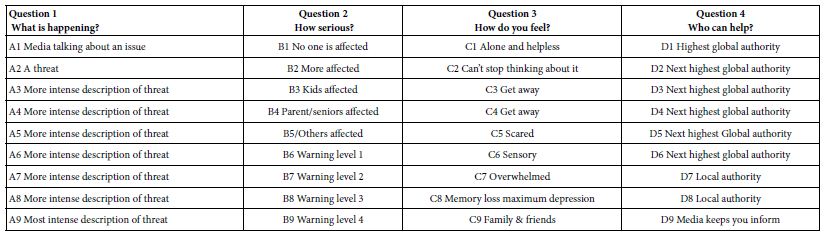
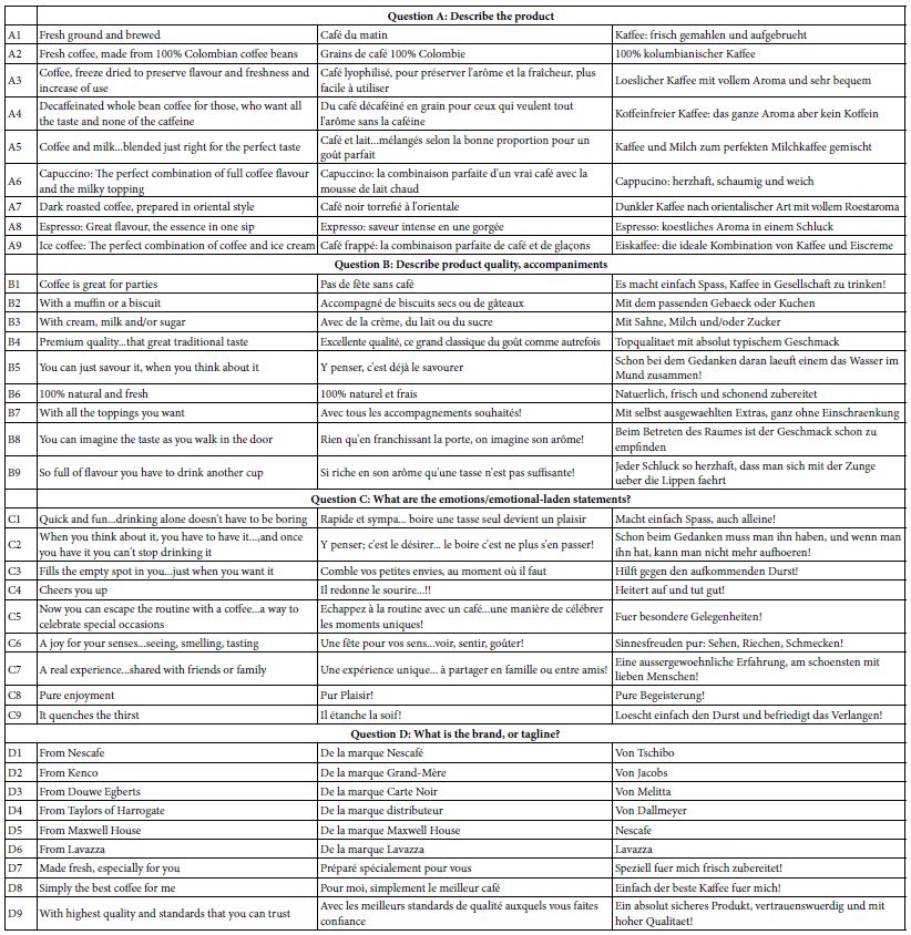
  1. The structure of the experimental design begins with a single topic (e.g., a social problem), continues with four questions dealing with the problem, and in turn uses four specific answers to each question. The three stages are easy to do, becoming a template. Good practice suggests that the 16 answers (henceforth elements) be simple declarative statements, each comprising 12 words or fewer, with no conjunctives. These declarative statements should be easily and quickly scanned, with as little ‘friction’ as possible.
  2. The specific combinations are prescribed by an underlying experimental design. The experimental design . The experimental design ensured that each element appeared exactly five times across the 24 vignettes, and that the pattern of appearances made each element statistically independent of the other 15 elements. A vignette could have at most one element or answer from a question. The actual design generates vignettes comprising a mixture of 4-element vignettes, 3-element vignettes, and 2-element vignettes, respectively, but never a 1-element vignette.
  3. The experimental design was set so that the data from each respondent, viz., the vignettes and their ratings, could be analyzed by ordinary least-squares (OLS) regression. That is, each respondent’s data comprised an entire experiment. The data could be analyzed in groups, or at the level of the individual. For this paper, the focus will be on the results emerging from the OLS regression at the level of each respondent.
  4. A key problem in experimental design is the focus on testing one specific set of combinations out of the large array of the underlying ‘design space’. The quality of knowledge suffers because only one small region of the design space is explored, usually that region believed to be the most promising, whether that belief is correct or not. . There is much more to the design space. The research resources are wasted minimizing the “noise” in this presumably promising region, either by eliminating noise (impossible in an Inner Psychophysics), or by averaging out the noise in this region by replication (a waste of resources).
  5. The solution of Mind Genomics is to permute the experimental design [15]. The permutation strategy maintains the structure of the experimental design but changes the specific combinations. The task of permuting requires that the four questions be treated separately, and that the elements within a question be juggled around but remain with the question. In this way, no element was left out, but rather its identification number changed. For example, A1 would become A3, A2 would become A4, A4 would become A2 and A3 would become or remain A3. At the initial creation of the permuted designs, each new design was tested to ensure that it ran with the OLS (ordinary least-squares) regression package. Each respondent ends up evaluating a different set of 24 combinations.
  6. The benefit to research is that research becomes once again exploratory as well as confirmatory, due to the wide variation in the combinations. It is no longer a situation of knowing the answer or guessing at the answer ahead of time. The answer emerge quickly. The data from the full range of combination tested quickly reveal what elements perform well versus what elements perform poorly.
  7. Continuing and finishing with an overview of the permuted design of Mind Genomics, it would be quickly obvious that studies need not be large and expensive. The ability to create equations or models with as few as 5-10 respondents, because of the ability to cover the design space, means that one can being to understand the ‘mind’ of people with so-called ‘demo studies’, virtually automatic studies, set up and implemented at low cost. The setup takes about 20 minutes once the ideas are concretized in the mind of the research. The time from launch (using a credit card to pay) to delivery of the finalized results in tabulated form, ready for presentation, is approximately 15-30 minutes.
  8. The final step, as of this writing (Fall, 2022), is to make the above-mentioned system work with a series of different studies of social problems, here, 27 studies. In the spirit of accelerated knowledge development, each study is a carbon copy of every other study, except for one item, the specific social issue addressed in the study. That is, the orientation, rating scale, and elements are identical. What differs is the problem. When everything else is held constant, only the topic being varied, we have then the makings of the database of the mind, done at industrial scale

Applying the Approach to the ‘Solution’ of Social Problems

We begin with a set of 27 social problems, and a set of solutions. The problems are ones which are simple to describe and are not further elaborated. In turn the 16 element or solutions are general approaches, such as the involvement of business, rather than more focused solutions comprising specific steps. The 27 problems are shown in Table 1, and the 16 solutions are shown in Table 2. For right now, it is just important to keep in mind that these problems and solutions represent a small number of the many possible problems one can encounter, and the solutions that might be applied. For this introductory study, using the Mind Genomics template, we are limited to four types of solutions for a problem, and four specific solutions each solution type. The number of problems is unlimited, however.

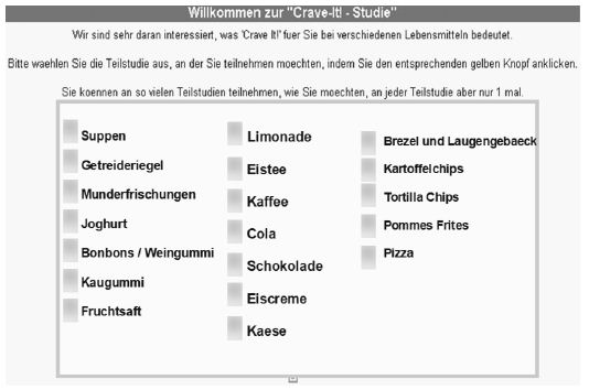
  1. Figure 1a and 1b shows two screen shots. Each problem is represented by a single phrase, describing the problem. That phrase is called ‘the SLUG’. In the figures, the words ‘ABORTION RIGHTS’ constitute the SLUG. The SLUG changes in each study, to present the topic of that study. There is no further elaboration of the topic as art of the introduction.
  2. The approach is templated, allowing the researcher to set up the study within 40 minutes, once the researcher identifies the social problem, creates the four questions, creates the four answers to each question (16 answers or elements), and then creates the rating scale. The researcher simply fills in the template as shown for one study, abortion, in Figure 1a and Figure 1b, respectively.
  3. Since the study is templated and of the precise same format except the topic, moving from one study to 26 copies becomes a straightforward task. The researcher copies the base study, but then changes the nature of the problem in the introduction, and the rating scale. This activity requires about 10 minutes per study. The activity simply requires the change of SLUGS. The total time for this ‘reproduction’ step is about two hours for the 26 remaining studies.
  4. Launch the 27 studies in rapid sequence. Each study requires about 1-2 minutes to launch, an effort accomplished in about one hour or less. The 27 studies run in parallel, each with about 50 respondents. With ‘easy-to-find’ respondents, the 27 steps take about two hours to run in the field, since they are running simultaneously, and require only a total of 1350 respondents.
  5. Using the ‘raw data’ files generated by the program, combine the raw data from the 27 studies into one comprehensive data file comprising all the data. Each respondent generates 24 rows of data. A study of one topic generates 24×50 or 1200 rows of data. The 27 studies generate 1200×27 rows of data. The effort to combine the data, ensuring that each study is properly incorporated into the large-scale database, requires about 2 hours.
  6. Convert the ratings so that ratings of 1-3 are converted to 0, to reflect the fact that the respondent does not feel that the combination of solutions will solve the social problem. Convert ratings of 4 and 5 to reflect the fact that the respondent does feel that the combination of solutions presented in the vignette will solve the social problem. Thus the ratings assigned by the respondent, a 5-point scale, are converted to a no/yes scale. To each converted value, viz., 24 binary values for each respondent, one per vignette, add a vanishingly small random number (~ 10-3). The small random number will not affect the results but will ensure variation in the newly created binary variable, (0=will not work, 100=will work). This type of conversion, viz., from a Likert Scale (multi-point category scale) to a binary scale, is a hallmark of Mind Genomics. The conversion comes from the history of consumer researchers and public opinion researchers working with YES/NO scales because managers do not understand what to do with averages of ratings. The averages have statistical meaning, of course, but have little built in meaning for a manager who has to make business decisions.
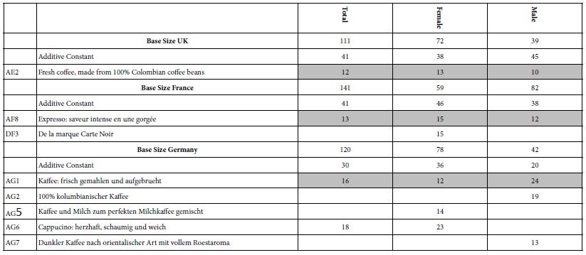
  7. Since the 24 vignettes evaluated by a respondent are created according to an underlying experimental design, we know that the 16 independent variables (viz., the 16 solutions) are statistically independent of each other. Create a model (equation) for each respondent relating the presence/absence of the 16 elements to the newly created binary variable ‘solve the problem.’ The equation does not have an additive constant, forcing all the information about the pattern to emerge from the coefficients. We express the equation as: Work (0/100) = k1(Solution A1) + k2(Solution A2) + …. K16(Solution D4). Each respondent thus generates 16 coefficients, the ‘model’ for that respondent. The coefficient shows the number of points on a 100-point scale for ‘working’ contributed by each of the 16 solutions.
  8. Array all the coefficients in a data matrix, each row corresponding to a respondent, and each column corresponding to one of the 16 solutions or elements. The data matrix is very large, comprising approximately 50 rows per study, one per respondent, and 27 blocks of rows, one block per study, to generate 1350 rows. Each row is unique, corresponding to a respondent, study, and comprises information about the respondent (age, gender, answer to classificaiton questions), and then the 16 coefficients.
  9. Cluster all respondents, independent of the problem topic, but simply based on the pattern of the 16 coefficients for the respondent. The clustering is called k-means [16]. The researcher has a choice of the measure of distance or dissimilarity. For these data we cluster using the so-called Pearson Model, where the distance between two respondents is based on the quantity (1-Pearson Correlation Coefficient computed across the 16 corresponding pairs of coefficients). Note that the clustering program ‘does not know’ that there are 27 studies. The structure of the data is the same from one study to another, from one respondent to another
  10. Each respondent is assigned to exactly one of the three large clusters (now called mind-sets), independent of WHO the person ‘is’, and the study in which the respondent participated. That is, the clustering program considers only the pattern of the coefficient. As a consequence, each of the three clusters can end up comprising respondents from each of the 27 studies. Finally, a respondent can be assigned to only one of the three clusters or mind-sets.
  11. Once the respondent is assigned to exactly one of the three mind-sets by the clustering program, the original raw data (24 rows of data for each respondent in each study) can now be augmented by an additional variable, namely the cluster membership of each respondent. The original raw data can be reanalyzed, first by total panel, then by mind-set, and then by mindset x study. With three mind-sets, there are now one grand equation with all the data, 27 equations for the 27 studies, and 81 equations for the 27 studies x 3 mind-sets.
  12. The analysis as outlined in Step 11 can be further strengthened by considering only those vignettes not rate ‘3’. Recall that ‘3’ corresponds to ‘cannot answer the question’. Eliminating all with ratings of ‘3’ eliminates these uncertain answers.
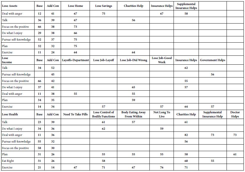
  13. The final data analytic step looks at the pattern of coefficients for the different groups (total, three mind-sets), considering the matrix of 16 elements (the solutions) x 27 studies. We will look only at strong performing elements, rather than trying to cope with a ‘wall of numbers’. For total panel, ‘strong’ is operationally defined as a coefficient of 25 or higher. For subgroups defined by the mind-sets, ‘strong’ is operationally defined as a coefficient of 30 or higher. These stringent criteria correspond to coefficients which are ‘statistically significant’ (P<0.05) through analysis of variance for OLS regression. All other coefficients will not be shown, in order to let the patterns emerge.
  14. The goal of the analysis is to get a sense of ‘what works’ for problems, solutions, and mind-sets. As we will see, most solutions fail to work for most problems. It is not that the solution is consciously thought to not work, but rather when the solution (an element) is combined with other elements, the patterns emerging suggest that the specific solution is simply irrelevant. As we will see, however, many solutions do work.
  15. The effort for one database, for one country, easy easily multiplied, either to the same database for different countries, or different topic databases for the country. From the point of view of cost, each database of 27 studies and 50 respondents per study can be created for $10,000 – $15,000, assuming that the respondents are easy to locate. That effort comes to about $400 – $500 per study. The time to create the database is equally impressive, days and weeks, not years.

Table 1: The 27 social problems. Each social problem was not further defined

table 1

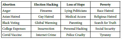
Table 2: The 16 solutions and their abbreviation in the data tables

table 2


fig 1a & 1b

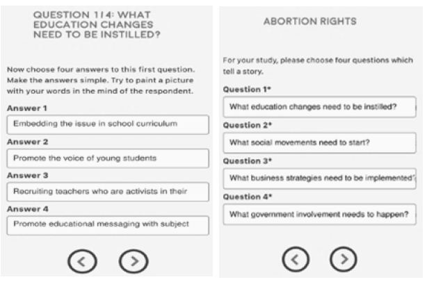
Figure 1a and 1b: Screen shots of the set up for one study (abortion rights)

Results for Total Panel and Three Emergent Mind-sets

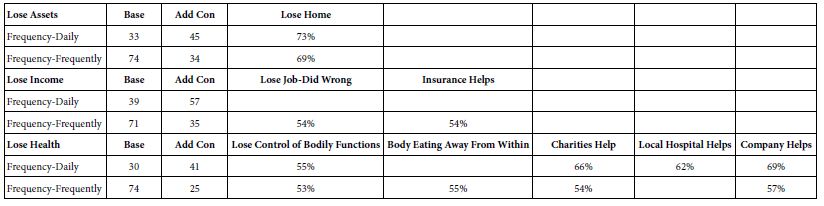
Let us now look at the data from the total panel. In its full form, Table 3 would show 16 columns ( one per each of the 16 solution or elements), and 27 rows (one row for each of the 27 problems). Recall from #13 above that the strong performing combinations of problem (row) and solution (column) are those with coefficients of +20 or higher. The strong performing combination correspond to significant likelihood of the solution solving the problem, across all respondents, but excluding those vignettes assigned a rating of ‘3’ (cannot decide).

Table 3: Summary table of coefficients for coefficients emerging from the model relating presence/absence of 16 solutions (column) to the expected ability to solve the specific problem (row). Models were estimated after excluding all vignettes assigned the rating 3 (cannot decide). Only strong performing elements are shown (viz., coefficient of 25 or higher)

table 3

Only 20 of the possible 432 problem/solutions are perceived as likely to ‘work’. The strongest performing solutions come from business. The strongest performing problem is parenting. The rest of the combinations which ‘work’ are scattered. Finally, five of the 16 solutions never work with any problem, and 15 of the 27 problems are not amenable to any solution.

One of the key features of Mind Genomics is the search for mind-sets. The notion of mind-sets is that for each topic area, one can discovered different patterns of ‘weights’ applied by the respondent to the information. For example, when it comes to purchasing a product, one pattern of weights suggests that the respondent pays attention to product features, whereas another pattern of weights applied to the same elements suggests that the respondent pays attention to the experience of consuming the product, or the health benefits of the product, rather than paying attention to the features.

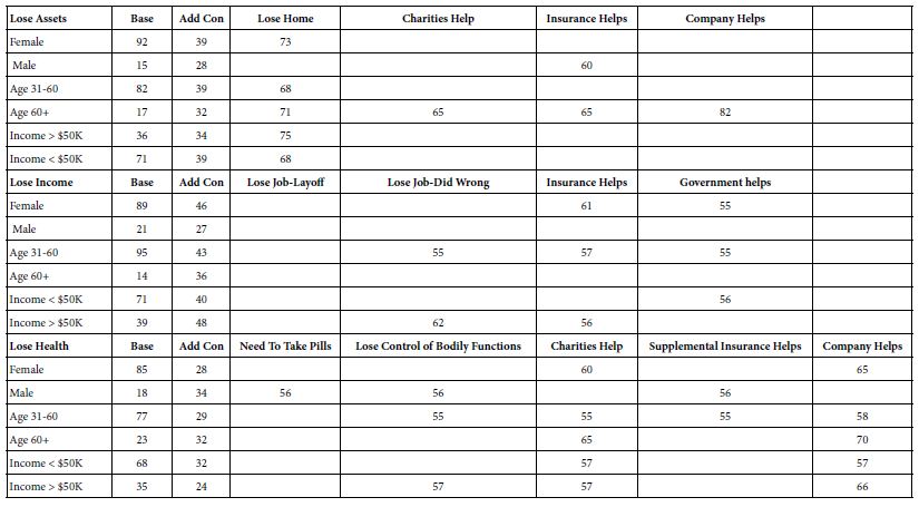
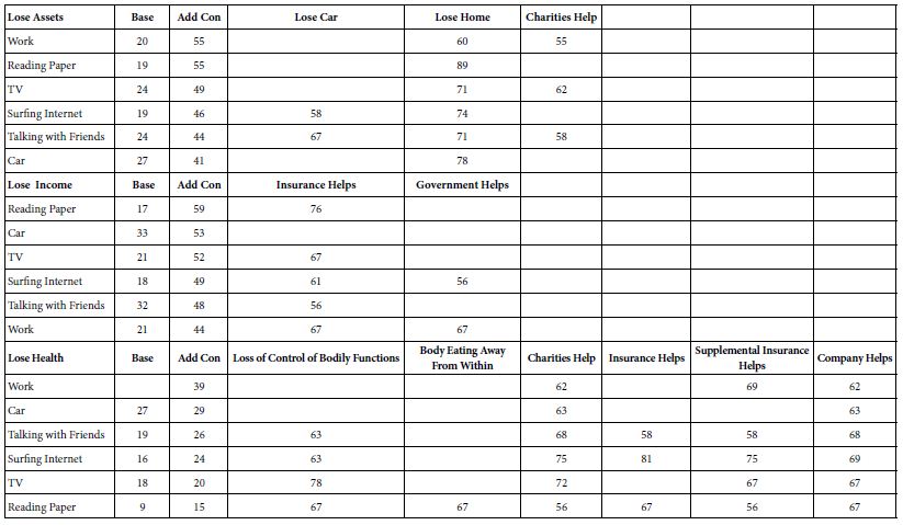
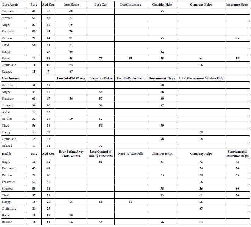
Our analysis proceeds by looking for ‘general’ mind-sets, across all 27 problems, and all 16 solutions. The coefficients for the three emergent mind-sets appear in Tables 4-6. Once again the only coefficients which appear in the tables are those coefficients deemed to be ‘very strong’ performers, this time with a value of +30 or higher. This increased stringency removes many coefficients. Yet, a casual inspection of Tables 4-6 shows that each table comprises more problems, more solutions, and more coefficients. The mind-sets do not believe that the key solutions will work everywhere, but just in some areas, in distinctly different areas, in fact. The mind-sets do not line up in an orderly fashion. That is, we do not have a simplistic set of psychophysical functions for the inner psychophysics. We do have patterns, and metrics for the social consensus.

  1. Mind-Set 1 (Table 4) appears to feel that business and education solutions will work more effectively than will solutions offered by government. Mind-Set 1 does not believe strongly in the public sector is able to provide workable solutions to many problems. Mind-Set 1 shows 46 problem/solution combinations of 30 or higher, and three problems/solutions combination with coefficients of 40 or higher. The 46 combinations are more than twice as many as the 20 combinations for strong performing elements from the Total Panel, even with the increased stringency applied to the mind-sets.
  2. Mind-Set 2 (Table 5) appears to feel that education and the law will solve many of the problems. Mind-Set 2 shows 50 problem/solution combinations of coefficient 30 or higher, and three combinations which show a coefficient of 40 or higher,
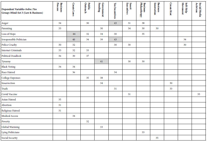
  3. Mind-Set 3 (Table 6) appears to feel that law and business will solve many of the problems. Mind-Set 3 shows 50 problem/solution combinations of coefficient 30 or higher, and five combinations which show a coefficient of 40 or higher,
  4. The increased richness of Tables 4-6 arises from the fact that the clustering isolates groups of individuals who think alike at the granular level of specific problems. By separating the mind-sets, the clustering program ensures that the individual coefficients have a less likely chance to cancel each other. We attribute the increased range to the hypothesis that people may be fundamentally different in their mental criteria. Inner Psychophysics reveals those differences, in a way that could not have been done before.

Table 4: Summary table of coefficients for model relating presence/absence of 16 solutions (column)to the expected ability to solve the specific problem (row). The data come from Mind-Set 1, which appears to focus on business and education, respectively, as the preferred solution to problems

table 4

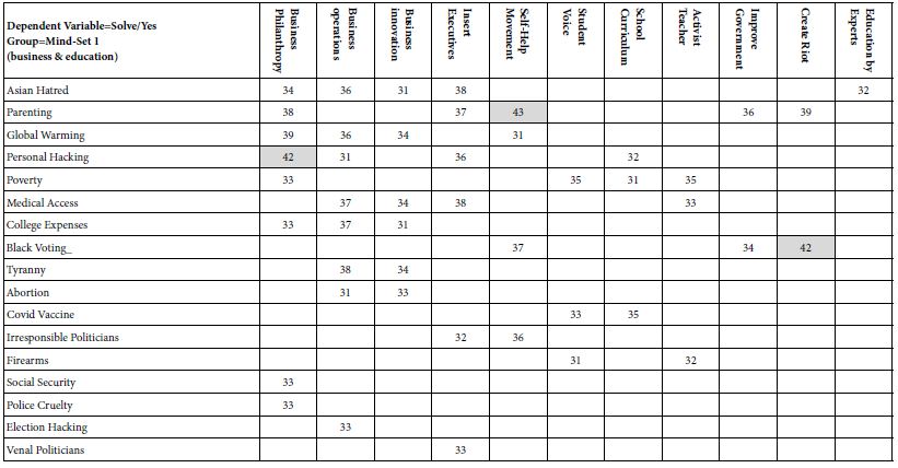
Table 5: Summary table of coefficients for model relating presence/absence of 16 solutions (column) to the expected ability to solve the specific problem (row). The data come from Mind-Set 2, which appears to focus on education and the law, respectively, as the preferred solution to problems

table 5

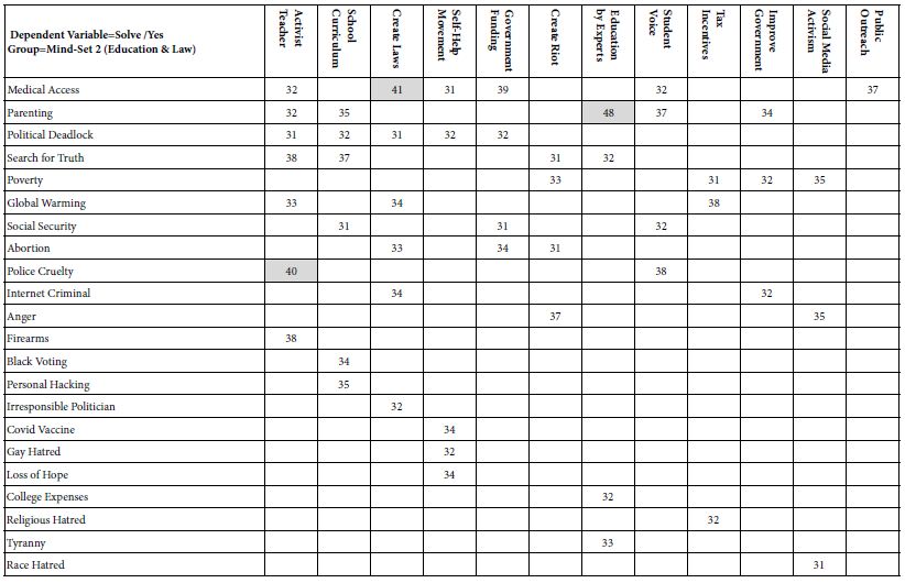
Table 6: Summary table of coefficients for model relating presence/absence of 16 solutions (column)to the expected ability to solve the specific problem (row). The data come from Mind-Set 3, which appears to focus on law and business, respectively, as the preferred solution to problems

table 6

The Inner Psychophysics and Response Time

Response time is assumed to reflect processes which occur. Longer responses times are presumed to suggest the involvement of more processes. So attractive is the study of response time as an indicator of internal processes that response time has moved from a simply a non-cognitive measure in behavior to a world of its own. Responses times are presented, along with hypotheses of what might be occurring [17]. Indeed, an entire division of applied consumer researcher has emerged to test ideas, the field being called implicit researcher after the work of Harvard psychologist Mazharin Banaji and her associates [18].

Let us take the same approach as above, relating the presence/absence of the 16 elements, not however to ratings of ability to solve the problem, but rather to the response time. The Mind Genomics program measured the number of seconds between the appearance of the vignette and the response assigned. When the respondent ‘dawdled’ in the self-pace experiment, the response time became unnecessarily long, for reasons other than reading and reacting. An operationally defined limit of six seconds was assumed for a participant. All vignettes with response times of nine seconds or longer were eliminated from analysis, as were all vignettes assigned the rating ‘3’ (cannot decide).

One might argue that by selecting data with responses times of 9 seconds or less, one is deliberately reducing the discrimination power of the analysis, by eliminating vignettes which required deliberation. This is correct removed a number of suspiciously long response times.

The Mind Genomics program then estimates the response time for each element (viz., solution) by using OLS (ordinary least-squares) regression. The equation is: Response Time = k1(A1) + k2(A2)…k16(D4). The equation is the same as the equations above for problem solving, other than the fact that there is no additive constant. The rationale for the absence of an additive constant is that the response time should be ‘0’ in the absence of any elements.

Table 7 shows the average coefficients for response times for three problems across 16 solutions. These problems are college expenses, COVID vaccination, and police cruelty. The average coefficients are shown by Total Panel, and then by three mind-sets. ‘Long’ response times (viz, high coefficients) of 2.0 seconds for an element (viz., solution) are shown by shaded cells. To allow the patterns to emerge, Table 7 presents only those coefficients which are 1.0 (seconds) or more.

Table 7: Estimated response times for specific elements, for the total panel and for the respondents in a defined mind-set. Only those response times for vignettes rating 1, 2, 4 or 5, were used in the computation. Only response times 9 seconds or shorter were used in the computation, under the assumption that longer response times meant that the respondent was multi-tasking

table 7

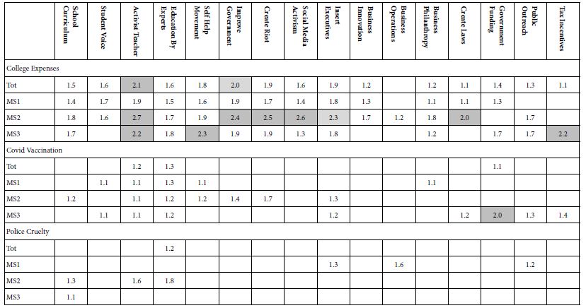
The pattern is obvious at the most general level…. People think about solutions when confronted with the topic of paying college expenses. People ponder the offered solutions. In contrast, there are fewer long response times for COVID vaccinations, and very few for Police Cruelty. In other words, it’s not only the solution, but rather the unique combination of problem and solution. We have here evidence of how the topic ‘controls’ attention.

Based upon the array of response times for elements shown in Table 7, we are left with the Herculean task of discovering an interpreting a coherent pattern, for Total Panel and then for mind-set. The pattern is, paradoxically, a lack of a pattern across mind-sets. That is, respondents may differ in what they believe will solve a problem, but difference in mind-sets does not manifest itself in the pattern of response times.

It is important to realize that the response times do not necessarily mean right or wrong, agree or disagree, and so forth. When confronted with data about Mind Genomics and its measurement of response time, the novice in Mind Genomics often asks whether a short response time (or conversely a long response time) is means that the person likes the topic, dislikes the topic, and so forth. We are so accustomed to judgments of dislike/like, bad/good, etc., that it is difficult to accept the fact that the response time (or other such metric, such as pupil size or galvanic skin response, GSR), are simply measures without any inherent meaning., viz., cognitively ‘poor.’ It is we who search for the meaning, wanting to contextualize observations of human non-conscious responses as clue to judgment, such as the extremely popular notion [19] patterns of thinking; System 1 (Fast) and System 2 (Slow Deliberate).

Discussion and Conclusion

The early work in psychophysics focused on measurement, the assignment of numbers to perceptions. The search for lawful relations between these measured intensities of sensation and a physical correlate would come to the fore even during the early days of psychophysics, in the 1860’s, with founder [20]. It was Fechner who would trumpet the logarithmic ‘law of perception, viz., that the relation between physical stimuli and perceived intensity was a logarithmic relation. One consequence of that effort to seek regularity in nature using one’s measures was to focus on the relationships between external stimuli and internal perceptions. This ‘external psychophysics’ focused on the search for lawful relationships that could be expressed by simple equations. The effort would be continued and brought to far more depth and application by Harvard professor S.S. Stevens, known as the father of modern psychophysics.

This paper began with the desire to extend psychophysics to the measurement of internal ideas The contribution of this paper is the introduction of a simple method for presenting stimuli, doing so in a way which forces the respondent to act as a measuring instrument, prevents biases, and emerges with numbers representing metrics of the mind. There are undoubtedly improvement that can be had, but the key aspects of the objective to ‘measure ideas’ (viz., the ‘inner psychophysics).

If we were to summarize the effort, we would point out these features:

A. The notion of isolating a variable and studying it in depth simply does not work when the nature of people is to think about ideas which are compound and complex. Traditional psychophysical methods simply are too unrealistic in view of the fact that the researcher cannot control the stimulus, the mind.

B. True to the word ‘psycho-physics’ which links two realms, the stimuli must be controlled by the researcher, and capable of systematic variation. If not, we are not true to the vision of psychophysics, linking two domains. The approach presented here, evaluation of systematically created combinations of stimuli, is consistent with the methods espoused by psychophysics.

C. The response should be a metric of ‘intensity’. The Likert scale presented here is such a scale. For science, the Likert scale data suffice. For application, most people have trouble interpreting the ‘implication’ of values on the Likert scale. That is, the scale is adequate, but most managers don’t really know the ‘practical meaning’ of the scale values. The transformation of Likert values to a binary scale ensures that the user of the information can make sense of the data.

D. The same type of study can be used to assess the impact of a set of ideas evaluated against different contexts. In the world of psychophysics, this type of study reveals the influence of different ‘backgrounds’ to affect the response to the stimulus (e.g., the perception of various coffees when the amount of milk is systematically varied). The psychophysical ‘thinking’ re-emerges when the topic or general problem is systematically varied across the 27 experiments, and then the study executed with new respondents. The outcome generates parallel sets of measures for ideas, each set pertaining to a specific topic, but everything else remaining the same.

E. Psychophysicists often look for explainable differences in the pattern of reactions to stimuli, more so in the chemical senses than in other areas, perhaps because in the chemical senses it is well known that people differ in what they like. This notion of basic groups, mind-sets, developed for simple stimuli in psychophysics, transfers straightforward to studies in Mind Genomics. Using the coefficients emerging from the OLS deconstruction of the rating at the level of the individual, one can find these ‘mind-sets’ for any specific topic, or as in this people, search for mind-sets which transcend the particular problem. Ability to cluster the respondents en masse, to create groups of individuals who show similar patterns of coefficients, viz., similar ways of thinking about solutions to problems.

Ability to measure the response time and determine whether we can discover any relation between response time as a well-known variable in psychology, and importance in decision making. The data emerging from this study suggest that the use of response times will not be particularly productive, except as a general measure. That is, we learn a great deal from the pattern relating ratings (more correctly transformed ratings) to the solutions. We learn a lot less by using response time in place of ratings. It may be that these relations exist, but are covered up by the richness of data, so that the basic patterns between text and response times are too subtle to be revealed in a study of this type.

References

  1. Stevens SS, Greenbaum HB (1966) Regression effect in psychophysical judgment. Perception & Psychophysics 1: 439-446.
  2. Stevens SS (1975) Psychophysics: Introduction to its Perceptual, Neural, and Social Prospects, Psychophysics, New York, John Wiley.
  3. Stevens SS (1966) A metric for the social consensus. Science 151: 530-541. [crossref]
  4. Boring EG (1942) Sensation and Perception in the History of Experimental Psychology. Appleton-Century.
  5. Galanter, E (1962) The direct measurement of utility and subjective probability. The American Journal of Psychology 75: 208-220. [crossref]
  6. Miller GA (1964) Mathematics and Psychology, John Wiley, New York.
  7. Luce, R. D., Bush, R. R., Galanter, E. (Eds.) (1963) Handbook of Mathematical Psychology: Volume John Wiley
  8. Luce RD, Tukey JW (1964) Simultaneous conjoint measurement: A new type of fundamental measurement. Journal of Mathematical Psychology 1: 1-27.
  9. Anderson NH (1976) How functional measurement can yield validated interval scales of mental quantities. Journal of Applied Psychology 61-677.
  10. Green PE, Srinivasan, V (1978) Conjoint analysis in consumer research: issues and outlook. Journal of Consumer Research 5: 103-123.
  11. Green, Paul E, Wind Y (1975) New Way to Measure Consumers’ Judgments. Harvard Business Review 53: 107-117.
  12. Wind, Y (1978) Issues and advances in segmentation research. Journal of Marketing Research 15: 317-337.
  13. Moskowitz HR, Kluter RA, Westerling, J, Jacobs HL (1974) Sugar sweetness and pleasantness: Evidence for different psychological laws. Science 184: 583-585. [crossref]
  14. Goertz G, Mahoney J (2013) Methodological Rorschach tests: Contrasting interpretations in qualitative and quantitative research. Comparative Political Studies 46: 236-251.
  15. Gofman, A, Moskowitz, H. (2010) Isomorphic permuted experimental designs and their application in conjoint analysis. Journal of Sensory Studies 25: 127-145.
  16. Dubes, R, Jain AK (1980) Clustering methodologies in exploratory data analysis. Advances in Computers 19: 113-228.
  17. Walczyk JJ, Roper KS, Seemann, E, Humphrey AM (2003) Cognitive mechanisms underlying lying to questions: Response time as a cue to deception. Applied Cognitive Psychology: The Official Journal of the Society for Applied Research in Memory and Cognition 17: 755-774.
  18. Cunningham WA, Preacher KJ, Banaji MR (2001) Implicit attitude measures: Consistency, stability, and convergent validity. Psychological Science 12: 163-170. [crossref]
  19. Kahneman, D (2011) Thinking, Fast and Slow. Macmillan
  20. Fechner GT (1860) Elements of Psychophysics Leipzig, Germany.
fig 4

Hypothalmic Hamartoma – A Rare Cause of Central Precocious Puberty

DOI: 10.31038/JCRM.2022553

Abstract

Hypothalamic hamartoma is a well-known neurological rare cause of central precocious puberty and gelastic seizures and may be asymptomatic for long period. It is rare and non-progressive tumor like congenital malformation. Precocious puberty defined as children attained the puberty before age of 8 years in girls and 9 years in boys. We present such a case of precocious puberty due to hypothalamic hamartoma in 5 year old boy and its radiological imaging findings.

Keywords

Hamartoma, hypothalamic, precocious, puberty, central cause

Introduction

Hypothalamic hamartoma is a rare non progressive tumor like well-organized congenital malformation of tuber cinereum in the floor of third ventricle [1-4]. It causes the classical spectrum or trait of gelastic seizures, precocious puberty and developmental delay or behavioral disorder [1,3]. It is most usual neurological cause of central precocious puberty.2 This condition may be asymptomatic for long period, or may present with clinical appearance and symptoms of precocious puberty and complex partial seizures refectory to anticonvulsant drugs [1,2]. One third of patients with hypothalamic hamartoma can be present with precocious puberty and it is defined as children attained the puberty before age of 8 years in girls and 9 years in boys [1,4,5]. Furthermore precocious puberty is divided into gonadotropin releasing hormone (GnRH)-dependent/central and gonadotropin releasing hormone (GnRH)-independent / peripheral precocious puberty [4]. Contrast enhanced MRI is investigation of choice and play important role in diagnosis of hypothalamic hamartoma [2,3] It appears as well-defined non enhancing lesion in floor of third ventricle showing similar signal intensity to the grey matter of brain parenchyma [3,4,6]. Gold standard treatment option for isolated central precocious puberty due to hypothalamic hamartoma is long acting analogs agonists of GnRH (GnHas) with good efficacy and safety [4,7].

Case Report

5 Years old boy came in paediatric outpatient department of Liaquat National Hospital with complain of faster growth of child than expected according to his father. On further questioning child has also history of epileptic laughter (gelastic seizures) 1-2 times, 2-3 months back for which he has taken antiepileptic drugs from local doctor in periphery of Afghanistan.

On local examination there were axillary and pubic hair and enlargement of penis measured about 4-5 cm in length. This was classified as TANNER stage (sexual maturity rating) 04 (Figure 1). Neurological examination was normal with Glasgow coma scale (GCS) of 15/15. Electroencephalogram (EEG) was recommended to see the cause of previous history of epileptic seizures was negative. His baseline laboratory investigations turned out to be within normal limits. On the basis of clinical and examination diagnosis of precocious puberty was made. His endocrinology related laboratory investigations were deranged. Follicle Stimulating Hormone (FSH) 4.11 (N= 1.9 mIU/ml), Luteinizing Hormone (LH) 9.82 (N1.3 mIU/ml) Testosterone 1500 ng/dL and Testosterone/Estradiol T/E2 ratio 45 pg/ml. All these investigations are raised and not normally corresponding to the patient’s age. Thyroid Function Tests (TFT) were within the normal limit.

fig 1

Figure 1: Enlarged penis and appearance of pubic hair not corresponding to the patient’s actual age

He underwent the contrast enhanced MRI brain which showed abnormal signal intensity mass arising from the tuber cinereum in the region of hypothalamus. It appeared iso-intense to grey matter on T1 and T2 weighted images and showed no post contrast enhancement. It measured about 0.9 x 1.1 cm. The lesion was very small in size and has no mass effect or compression over the adjacent brain parenchyma. This was diagnosed as hypothalamic hamartoma. (Figures 2 and 3). Patient also underwent the X-ray right hand and elbow according to the radiological protocol to see the exact age of patient which showed 15 years reported by the experienced radiologist (Figure 4). During hospital stay course patient was asymptomatic and discharged on long acting analogs agonists of GnRH (GnHas). Follow-up was recommended in outpatient department of endocrinology.

fig 2

Figure 2: A Axial T2 weighted image and B sagittal T2 weighted image show abnormal signal intensity mass arising from the tuber cinereum in the region of hypothalamus. It appears iso-intense to the brain parenchyma (black arrow head)

fig 3

Figure 3: A sagittal plain T1 weighted image and B sagittal contrast enhanced T1 weighted image show abnormal signal intensity mass arising from the tuber cinereum in the region of hypothalamus. It appears iso-intense to brain parenchyma and show no post contrast enhancement (White arrow head)

fig 4

Figure 4: A anterior-posterior elbow, B lateral elbow and C anterior-posterior wrist X-rays show bone age of 15 years

Discussion

Previously Hypothalamic hamartoma used to be an uncommon finding and was estimated to occur in one person per one million population,1 however with timely advancement in the field of Radiology and better clinical recognition, the early diagnosis has now become possible and its incidence has significantly decreased [1,2].

Most patients usually present in the first or second decade of life [1-3]. Precocious puberty is the most common presentation, however larger hamartomas are less likely to produce precocious puberty [2,3]. Other clinical presentations include developmental delay, attention deficit or hyperactivity disorder and anxiety [1-4]. A very specific feature of hypothalamic hamartoma is Gelastic seizure [1-3]. In our case, hamartoma measured up to 1cm on MRI brain (Figure 2) and patient was presented with complaints of both precocious puberty and laughing fits (Gelastic seizures).

On MRI, hypothalamic hamartomas produce soft tissue intensity masses which are isointense to grey matter on T1WI and hyperintense on T2WI [2,3]. They are homogeneous and sharply marginated by the surrounding CSF with no post contrast enhancement [2,3,6]. Calcification is rare and hemorrhage is not described in these lesions [2,3]. This classical appearance of soft tissue intensity mass in the region of hypothalamus was also observed in our patient (Figure 2).

Patients with central precocious puberty are usually managed conservatively [2], for progressive central precocious puberty, treatment with a depot GnRH agonist is suggested and is generally continued for 11 years [2-4]. However, surgery including resection or disconnection through craniotomy or trans-spheroidal approach can be helpful in cases of poorly controlled epilepsy [2-6], to our patient, we advised long acting analogs agonists of GnRH (GnHas) with a follow up in OPD.

Conclusion

Hypothalamic hamartomas are rare congenital malformation seen in floor of third ventricle. Precocious puberty is most usual presenting feature. MRI brain play important role in diagnosis of these lesions. Radiologist should aware of imaging findings of hypothalamic hamartoma and should examine the hypothalamic region properly in suspected cases as they can be easily missed due to small size. Bone age can be assessed by using the wrist X-ray and we can also observe the slowing of bone growth after treatment by X-ray wrist recommendation in every 6th month.

References

  1. Qasim BA, Mohammed AA (2020) Hamartoma of hypothalamus presented as precocious puberty and epilepsy in a 10-year-old girl. International Journal of Surgery Case Reports 77: 170-173. [crossref]
  2. Mahmood R, Al Taei TH, Samah Al Obaidi MD (2019) Hamartoma of the Hypothalamus. Bahrain Medical Bulletin 41.
  3. Kalekar T (2015) Hypothalamic Hamartomas: Two Cases. Open Journal of Medical Imaging 5: 20.
  4. Sharma P, Acharya N, Guleria TC (2020) Hypothalamic hamartoma presenting as central precocious puberty: a rare case report. International Journal of Contemporary Pediatrics 7: 1634.
  5. Mahajan ZA, Mehta SR (2020) Central precocious puberty: A case report. Medical Journal of Dr. DY Patil Vidyapeeth 13: 413.
  6. Boyko OB, Curnes JT, Oakes WJ, Burger PC (1991) Hamartomas of the tuber cinereum: CT, MR, and pathologic findings. American Journal of Neuroradiology 12: 309-314. [crossref]
  7. Eugster EA (2019) Treatment of central precocious puberty. Journal of the Endocrine Society 3: 965-972. [crossref]
fig 5

Arizona Reopening Phase 3 and COVID-19: After 18 Months

DOI: 10.31038/JCRM.2022544

Abstract

There had been three Arizona COVID-19 Reopening Phases. On March 5, 2021, Arizona’s Reopening Phase 3 began. The state is the sixth largest in size of the United States 50 states and about the same size as Italy. There were four case surges — in the summer and fall 2021 with Delta variant, and the winter 2021-22 and summer 2022 with Omicron variants. This 18 months longitudinal study examined changes in the number of new COVID-19 cases, hospitalized cases, deaths, and vaccinations. There was an increase of more than 1.4 million cases during the study period. The data source used was from the Arizona Department of Health Services COVID-19 dashboard database. Even with the case surges, the new normal was low number of severe cases, manageable hospitalization numbers, and low number of deaths.

Keywords

COVID-19, Arizona returning to normal, Longitudinal study, Arizona and COVID-19

Introduction

The severe acute respiratory syndrome coronavirus 2 (SARS-CoV-2) is also known as COVID-19 (coronavirus). It is a respiratory disease (attacks primarily the lungs) that spreads by person to person through respiratory droplets (coughs, sneezes, and talks) and contaminated surfaces or objects. Since the virus first appears in Wuhan, China in December 2019, there has been more than 600 million cases in the world. On September 7, 2022, Johns Hopkins University [1] reports that there are 606,889,445 total COVID-19 cases and 6,507,958 deaths associated with the virus in the world. The United States has the highest total cases (95,020,855) and deaths (1,048,989) in the world [1].

A three prolong attack is used against the virus by encouraging the public to practice preventive health behaviors that reduces the risks of getting respiratory infections (e.g., coronavirus, flu, and cold), and using vaccines and therapeutics. The preventive health behaviors include, but not limited to, practicing physical and social distancing, washing hands frequently and thoroughly, and wearing face masks. Johns Hopkins reports that more than 12.18 billion vaccine doses have been administered in the world and the U.S. has administered more than 605 million vaccine doses (September 7, 2022) [1].

There has been three Arizona Reopening Phases. During Arizona’s Reopening Phase 2 winter surge in 2020, ABC and NBC News report that the state has the highest new cases per capital in the world [2,3]. On September 7, Arizona is ranked 12th in total COVID-19 cases (2,258,040) and 11th in total deaths (31,162) of the 50 U.S. states [1]. Arizona is the sixth largest in size (113,990 square miles / 295,233 square kilometers) of the U.S. 50 states and is about the same size as Italy (301,340 square kilometer) [4,5]. The state population estimate is 7,276,316 on July 1, 2021 [6].

A partnership between the U.S. federal government and each of the 50 states is required to address the COVID-19 pandemic [7,8]. The federal government provides the national guidance primarily through the Centers for Disease Control and Prevention (CDC) and needed logistical support (e.g., provide federal supplemental funding, needed medical personnel and resources, and other needed assistance). The states decide on what actions to take and when to carry out those actions; the state COVID-19 restrictions; when to carry out each reopening phase; and the state vaccination plan.

On March 5, 2021, Arizona Governor Douglas Ducey begin Reopening Phase 3 (final reopening phase) after the state had administered more than two million vaccine doses and several weeks of declining cases [9,10]. This eases more of the COVID-19 restrictions. As more people become vaccinated and those infected recovered and have immunity against the virus; the numbers of cases, hospitalizations, and deaths will be low; COVID-19 will be manageable; and the state returns to normal.

The remainder of the paper examines Arizona Reopening Phase 3 (March 5, 2021 to September 7, 2022) looking at changes in the number of new COVID-19 cases, hospitalizations, and deaths.

Methods

This was an 18-months longitudinal study. The Arizona Department of Health Services (the state health department) COVID-19 dashboard database was the data source used. The study examined the changes in the numbers of new COVID-19 cases, hospitalized cases, deaths, and vaccines administered.

There were several data limitations. The COVID-19 case numbers represented the numbers of positive tests reported. When more than one test given to the same person (e.g., during hospitalization, at work, and mandatory testing), there were individual case duplications. Aggressive testing resulted in increases in false positive and false negative testing results. The case numbers did not include positive home testing results.

Delays in the data submitted to the state health department affected the timeliness of data reported and caused fluctuations in the number of cases, hospitalizations, deaths, and vaccinations. The state health department continued to adjust the reported numbers that may take more than a month to correct the numbers. The deaths associated with the coronavirus may cause by more than one serious underlying medical conditions, and the virus may not be the primary cause of death.

Results

A case could be mild (no symptoms), moderate (sick, but can recover at home), and severe (require hospitalization and/or result in death). There were four case surges during the Reopening Phase 3: 2 summers, 1 fall, and 1 winter. The 2022 cases (882,671) had already exceeded the 2021 total case numbers (838,836). Figure 1 shows the Arizona weekly COVID-19 cases during January 1, 2020 to September 10, 2022.

fig 1

Figure 1: Arizona Weekly COVID-19 Cases: January 1, 2020 to September 10, 2022.
Source: Arizona Department of Health Services Arizona COVID-19 weekly Cases Graph*2022 cases as of September 14.

At the end of the 18 months of Arizona Reopening Phase (began March, 5, 2021), there were 1,432,921 COVID-19 cases, 59,091 case hospitalizations, and 14,839 deaths associated with the virus in Arizona (Table 1). There were higher percentages of hospitalizations, and deaths in the first 6 months of the first year than the following two 6-month periods.

Table 1: Arizona Reopening Phase 3 Total Numbers of COVID-19 Cases, Hospitalizations, and Deaths: March 7, 2021 to September 7, 2022

table 1

Source: Arizona Department of Health Services COVID-19 Dashboard.
Arizona 2021 population estimate is 7,276,316, July 1, 2021 – U.S. Census.

Table 2 tracks the weekly total and weekly numbers of COVID-19 cases, hospitalized cases, and deaths during the past 6 months (March 9 through September 7, 2022). The largest weekly numbers of cases (20,198) occurred on July 6, while hospitalizations (1,955) occurred on March 9. The largest weekly number of deaths was on March 16 (457).

Table 2: Arizona Total and Weekly Numbers of COVID-19 Cases, Hospitalizations, and Deaths

table 2

Source: Arizona Department of Health Services COVID-19 Dashboard.
Arizona 2021 population estimate is 7,285,370, July 1, 2021 – Arizona OEO.

Figures 2-4 compare the numbers of COVID-19 cases, hospitalized cases, and deaths by age groups for the three 6-month periods. A case could be mild, moderate, and severe. Most people recovered and did not require hospitalization. There was an increase of 1,432,921 cases during the 18 months. The 20-44 years age group had the largest number of cases (Figure 2). There were more females (52.8%) than males (47.2%) who got the virus on September 7, 2022.

fig 2

Figure 2: Arizona Reopening Phase 3 COVID-19 Cases by Age Groups for Three 6-Month Periods.
Source: Arizona Department of Health Services COVID-19 Cases by Age Groups Statistics.

The percentages of total hospitalized cases (severe cases) decreased from 7 percent on March 6, 2021 to 5 percent on September 7, 2022. The case hospitalizations had increased by 59,091 during the study period. Seniors had the highest percent of the total hospitalizations (43.7% on September 7) and those under 20 years of age had the lowest percent (4.5%). Eighteen percent (18.1%) of seniors diagnosed with COVID-19 hospitalized, while 1.1 percent of those under 20 years of age hospitalized. There were more males (52.2%) than females (47.8%) hospitalized. Figure 3 shows the hospitalization numbers for each age group with the virus for the three 6-month periods.

The numbers of deaths had increased by 14,839 during the 18 months. The rates of fatalities per 100,000 population increased 227.05 to 433.50. As expected, seniors had the highest percent of total deaths (71.3% on September 7) and those under 20 years of age had the lowest percent (0.2) Eight percent (7.9%) of the seniors diagnosed with COVID-19 died, while 0.01 percent of those under 20 years of age died. There were more males (59%) than females (41%) who died. Figure 4 shows the numbers of deaths for each age group with the virus for the three 6-month periods.

The first U.S. COVID-19 vaccine, Pfizer/BioNTech Comirnaty, approved for emergency use authorization on December 11, 2020. In late December, Arizona began to administer vaccines. During Reopening Phase 3 (March 5, 2021 to September 7, 2022), there were 10,451,502 vaccine doses administered, and 3,813,974 fully vaccinated against the virus. Figure 5 shows the numbers of COVID-19 vaccines that were given in Arizona (persons fully vaccinated, persons receiving at least one dose, and total doses given) during the 18 months.

Initially, there were three vaccines available (Pfizer/BioNTech Comirnaty, Moderna Spikevax, and Johnson&Johnson Jcovden). Novavax Nuvaxivud became the fourth vaccine available in July 2022. The vaccines provided different levels of protection against COVID-19 and its variants. Those 65 years and older had the highest vaccination percentage, while those under 20 years of age had the lowest (Figure 6). It was expected the vaccination rates for this age group will increase with the approval of younger children vaccines use.

fig 3

Figure 3: Arizona Reopening Phase 3 Hospitalized COVID-19 Cases by Age Groups for Three 6-Month Periods.
Source: Arizona Department of Health Services Hospitalized COVID-19 Cases by Age Groups Statistics.

fig 4

Figure 4: Arizona Reopening Phase 3 COVID-19 Deaths by Age Groups for Three 6-Month Periods.
Source: Arizona Department of Health Services COVID-19 Deaths by Age Groups Statistics.

fig 5

Figure 5: Arizona Reopening Phase 3 COVID-19 Vaccination Numbers: March 5, 2021 to September 7, 2022.
Source: Arizona Department of Health Services COVID-19 Vaccination Statistics.

fig 6

Figure 6: Arizona COVID-19 Vaccination Percentages (at least one dose) by Age Groups on September 7, 2022.
Source: Arizona Department of Health Services COVID-19 Vaccinations by Age Group Statistics.

Discussion

The Arizona Governor began Reopening Phase 3 (final phase of reopening) after the state had administered more than two million vaccine doses and several weeks of declining cases on March 5, 2021 [9,10]. The state continued its efforts to vaccinate its population. The number of vaccine dosages administered had increase from 2,016,512 on March 5, 2021 to 12,468,014 on September 7, 2022. Sixty-two percent (4,525,048) of the state population were fully vaccinated. The largest numbers of fully vaccinated persons occurred in the week of April 17 to 23, 2021 (249,755) [9,10]. The pace of vaccination began to slow down in June.

Arizona case numbers had decreased in the spring and early summer 2021. At the end of June, the Arizona State Legislature and Governor had rescinded many of the state COVID-19 restrictions. The state used a three-pronged attack against the virus: (1) encourage preventive health behaviors, (2) increase vaccination numbers, and (3) use therapeutics. During the month of July, the highly contagious Delta variant appeared in the state and began the summer surge. Even with the increase vaccination efforts and other actions, they were not enough to stop the Delta variant. This resulted in the fall surge.

In December, the more contagious Omicron variant appeared in the state and began to surge. The Omicron variant surge in January 2022, and the cases remained high into early March. For more than two months in the spring, the cases were low. The state cases rose at the end May as the Omicron variants moved westward in the U.S. and began the summer surge. By late August, the cases declined.

It has been more than 32 months since the first COVID-19 cases appeared in Arizona on January 22, 2020; the state has not returned to pre-pandemic normal of zero cases and no face mask wearing. Most health facilities require both medical staff and patients wear masks. Many businesses require their staff wear masks and masking wearing is optional for customers, and they still have their virus protective glass/plastic barriers. There are signs of the public experiencing COVID fatigue (e.g., significant numbers did not wear masks during summer 2022 case surge and did not pay attention to the daily/weekly number of case increases).

Many still have anxiety/depression/stress associated with the virus. The causes for the mental anguish are the uncertainty of the virus, constant emergent of new variants, vaccine limitations, the lack control of the situation, and no end to the virus. There are persons who have not adapt to the new normal and have limited their interactions with people.

Overtime, the vaccines are not as effective against the later variants (Delta and Omicron) and Omicron subvariants as the original Alpha – breakthrough infections and wane over time. Even though the vaccines and their boosters reduce the risks in getting a severe case, one can still can get the virus. There has been very little increase in the vaccination rate in the last six months — the number of fully vaccinated percent increased only by 2.9 percent.

The Food and Drug Administration has approved both Pfizer and Moderna new bivalent COVID-19 vaccines that are effective against both the original virus and Omicron BA.4 and BA.5 variants on August 31, 2022. With the new vaccines, it is expected the vaccination rates will rise; the population immunity level will be high enough to keep the winter case surge lower than last year; and the state will move the closer to returning back pre-pandemic normal.

Conclusion

The vaccines, most of the Omicron variant cases are mild or moderate, and therapeutics have kept the number of hospitalizations and deaths low. Even with the occasion case surges, the state new normal are low number of severe cases, manageable hospitalization numbers, and low number of deaths.

References

  1. Johns Hopkins University Coronavirus Resource Center, https://coronavirus.jhu.edu/.
  2. Deliso, Meredith. “Arizona ‘hottest hot spot’ for COVID-19 as health officials warn of hospital strain: The state has the highest infections per capita globally, based on JHU data, ABC News, January 7, 2021, https://abcnews.go.com/US/arizona-hottest-hot-spot-covid-19-health-officials/story?id=75062175.
  3. Chow, Denise and Joe Murphy. These three states have the worst Covid infection rates of anywhere in the world: Arizona currently has the highest per capita rate of new Covid-19 infections, with 785 cases per 100,000 people over the past seven days, followed closely by California and Rhode Island, NBC News, January 5, 2021 and updated on January 7, 2021, https://www.nbcnews.com/science/science-news/these-three-states-have-worst-covid-infection-rates-anywhere-world-n1252861.
  4. Britannica, Arizona state, United States, https://www.britannica.com/place/Arizona-state.
  5. My Life Elsewhere, Arizona is around the same size as Italy, https://www.mylifeelsewhere.com/country-size-comparison/arizona-usa/italy.
  6. United States Census Bureau, Quick Facts, https://www.census.gov/quickfacts/AZ.
  7. Eng H (2020) Arizona and COVID-19. Medical and Clinical Research 5: 175-178.
  8. Eng H (2021) Arizona Reopening Phase 2: Rise and Fall of COVID-19 Cases. Medical and Clinical Research 6: 114-118.
  9. Eng H (2021) Arizona Reopening Phase 3 and COVID-19: Returning to Normal. Medical and Clinical Research 6: 687-669.
  10. Eng H (2022) Arizona Reopening Phase 3 and COVID-19: One Year Later. Journal of Clinical Research and Medicine 5: 1-7.

Anxiety, Stress, Depression among School Going Adolescents in Bareilly City: A Cross Sectional Study

DOI: 10.31038/PSC.2022221

Abstract

Context: Depressive disorders often start at a young age. There is a need for early identification of depression, anxiety, and stress (DAS) and prevention. The present study was undertaken to find the magnitude of DAS among adolescents.

Aims: To find the mental health status of school going adolescents in Chandigarh. The objectives were (i) to study the prevalence of DAS among school going adolescents and (ii) to study the correlates of DAS. Settings and Design: A Cross‑sectional survey of students of four classes from 9th to 12th studying in government schools.

Subjects and Methods: Ten government schools in Bareilly City were randomly selected through lottery method. In each school, for each of the four classes, a section was randomly selected again by the lottery method. Forty students were selected from each school reaching sample size of 470. DAS scale 21 questionnaires were used.

Statistical Analysis Used: The data entry was done in MS Office Excel 2007. The analysis was done in the form of frequency tables, charts cross tables. For statistical significance, Chi‑square test and correlation was found between various factors.

Results: The prevalence of DAS was 65.53%, 80.85%, and 47.02%, respectively. Overall, comorbidity between depression and anxiety was 57.65%. Extremely severe depression was very less (3%). The prevalence of DAS was higher in females. For depression and anxiety, the peak age was 18 years. Conclusions: The prevalence of DAS was high among school going adolescents in Bareilly City. There is a need for early and effective identification of DAS that can prevent many psychiatric disorders at their nascent stage.

Keywords

Adolescent, Depression, Anxiety, Stress, Bareilly City

Introduction

Mental illnesses account for a significant share of the disease burden in all civilizations. Depression, anxiety, and stress are among the most common causes of illness and disability in children. Teenagers are predisposed to a range of mental health difficulties due to the physical, psychological, and behavioral variations during this time. Poor academic performance, lack of communication with friends and family members, substance misuse, feelings of abandonment, homicidal thoughts, and suicide ideation are all signs of these three diseases [1,2].

For at least two weeks, depression is defined by persistent unhappiness and a loss of interest in activities that you generally love, as well as incapacity to function in everyday life. Anxiety is a sensation of tension accompanied by concerned thoughts and bodily changes such as elevated blood pressure. Anxiety disorders are characterized by recurrent intrusive thoughts or concerns.

Nearly 20% of children suffer from a diagnosable mental illness. In addition, numerous mental health illnesses emerge during adolescence. Before reaching adulthood, between 20-30% of children will experience at least one significant depressive episode. For a quarter of people, mood disorders such as depression first appear throughout adolescence. Anxiety disorders and impulse control disorders (such as conduct disorder or attention deficit/hyperactivity disorder) affect 50-75 percent of adolescents during their adolescence. As children enter puberty, existing mental health issues become more complex and acute. Adolescents with untreated mental health issues are more likely to perform poorly in school, drop out, have strained family connections, abuse substances, and engage in risky sexual practices [3].

Being away from home, grade, stream of study, academic performance and examination-related concerns, and cyber bullying have all been connected to depression in previous studies. According to earlier studies, sex, grade level of pupils, and kind of school (public or private), family type, not living with parents, educational level of parents, and high academic stress were all factors of anxiety.

Globally, depression is one of the leading causes of illness and disability. Even in developed nation’s depression is a known health burden among children, adolescents, and adults. One in four children in the age group of 13-15 years in India suffers from depression, which affects 86 million people in the South-East Asia region, the World Health Organization. In adolescents, major depression is projected to rank second-most cause of human illness by the year 2020 [4,5].

To battle the burden of juvenile mental health concerns, researchers must investigate the extent and risk factors of symptoms of depression, anxiety, and stress. Nevertheless, anxiety and depression in early teens commonly go undetected and untreated, particularly in developing countries like India, due to limited access to psychological and psychiatric care as well as the enormous societal stigma regarding mental health concerns. Keeping these points in mind, an attempt will be made to assess the depression, anxiety and stress among school students in Bareilly City, Uttar Pradesh.

Materials and Methods

The A cross sectional research was carried out among school students in Bareilly city from February 2022 – April 2022. The study was approved by the Institutional Review Board, Institute of Dental Sciences, Bareilly. Prior beginning the research, the production lines head provided written approval for it to be carried out there. Sample size has been scientifically estimated using G Power V 3.1 Software which yielded a minimum sample size of 470 School students. School students who were aged 10-19 years and whose parents will give consent to allow their children to participate were included in the study. School going children whose parents are not willing to give consent and who are likely to take transfer during the study period and those who did not want to take part in this research were eliminated. Multistage sampling technique was used for all the study units until the required sample size is attained.

The complete information about the study will be informed to the participants as mentioned in the participant information sheet. Signed informed consent form will be obtained from all the participating subjects after explaining the complete procedure in their vernacular language. A pre-designed semi-structured, self-administered questionnaire was used to assess socio-demographic profile like age, gender, religion etc. and associated factors like pressure to perform, relations with parents etc. Depression anxiety stress scale (DASS)-21 was used to detect depression, anxiety and stress.

Statistical Analysis

Data was entered on Microsoft excel software and statistical analysis was done using a licensed version of SPSS 21. Descriptive analysis was done by calculating proportions, means and standard deviation.

Results

Out of 470 students, the maximum number of students participating in study was from 9th class (28.72%), and minimum number of students was from 12th class (22.76%). There were 257 male (54.68%) and 213 female (45.31%) participants in the study. The maximum number of students were from the age group of 16 years, i.e., 180 (38.29%) and minimum from the age group of 19 years, i.e., 3 (0.63%) students. Table 1 shows gender‑wise distribution of participants having DAS. Table 2 shows that overall comorbidity between all three disorders, i.e., DAS was 36.1%. Distribution of participant and 12th class having the DAS is shown in Table 3. On comparison of DAS among participants of 9th, 10th, 11th, 12th classes, it can be seen that depression was higher in 12th class, anxiety was higher in 10th class, and stress was higher in 9th class. While comparing DAS among participant of nonboard (9th + 11th) and board classes (10th + 12th), it was found that it was higher in board classes than in nonboard classes. It was found that all types of depression (75.59%) and stress (53.52%) were higher in board classes than of nonboard classes (57.2% and 41.63%,respectively).Among students of classes 11th and 12th, according to their stream, it was found that depression and anxiety were maximum in medical students (78.57%), and stress was more in commerce students (48.89%). It was found that extremely severe depression was highest among medical students (03.57%); mild depression was also more in them (28.57%). Moderate depression was more in arts students (43.42%). Extremely severe (17.10%) and moderate anxiety (27.63%) were higher in arts students. Mild anxiety was higher in medical students (42.86%). Severe anxiety was higher in commerce students (16.67%). Extremely severe stress was present only in commerce students (01.11%); severe stress was higher in nonmedical students (60.71%). Mild stress was higher in arts students (35.53%).

Table 1: Gender wise distribution of participants having depression, anxiety, and stress (n=470)

Gender

Number of students

Prevalence of DAS (%)

Males

257

85 (33.07)

Females

213

85 (39.9)

DAS: Depression, anxiety and stress

Table 2: Comorbidity between different disorders (n=470)

Comorbidity

n (%)

Overall

170 (36.17)

Depression and anxiety

271 (57.65)

Depression and stress

144 (40)

Stress and anxiety

200 (50)

Table 3: Distribution of participants of 9th, 10th, 11th and 12th class having the depression, anxiety, and stress (n=470)

Students of class

DAS Normal (%) Mild (%) Moderate (%) Severe (%)

Extremely severe (%)

Class 9th (n=135) Depression

55 (40.74)

21 (15.56) 40 (29.63) 14 (10.37)

5 (3.7)

  Anxiety

37 (27.41)

31 (22.96) 52 (38.52) 14 (10.37)

1 (0.74)

  Stress

32 (23.7)

37 (27.41) 51 (37.78) 9 (06.67)

6 (4.44)

Class 10th (n=106) Depression

28 (26.42)

27 (25.47) 32 (30.19) 14 (13.21)

5 (4.72)

  Anxiety

18 (16.96)

21 (19.81) 39 (36.79) 15 (14.15)

13 (12.26)

  Stress

50 (47.17)

30 (28.30) 10 (09.43) 15 (14.15)

1 (0.94)

Class 11th (n=122) Depression

55 (45.08)

20 (16.39) 34 (27.87) 12 (09.84)

1 (0.82)

  Anxiety

27 (22.13)

36 (29.51) 26 (21.31) 21 (17.21)

12 (09.84)

  Stress

72 (59.02)

29 (23.77) 11 (09.02) 9 (07.38)

1 (0.82)

Class 12th (n=107) Depression

25 (23.30)

23 (21.36) 43 (40.78) 12 (11.65)

4 (02.91)

  Anxiety

21 (19.42)

29 (27.18) 25 (23.30) 12 (11.65)

20 (18.45)

  Stress

49 (45.63)

40 (37.86) 6 (05.83) 12 (10.68)

0

DAS: Depression, anxiety and stress            

Self-satisfaction with academic performances in participants with DAS was 67.08%, 86.07%, and 40.5%, respectively whereas the parent’s satisfaction with academic performances of their wards with DAS was 66.86%, 80.47%, and 43.19%, respectively. Poor socioeconomic conditions and father’s occupation (nonworking) were directly related with higher level of DAS. With increase in the education level of parents, level of DAS in their children decreased. As the parents love decreased, level of depression and stress in the participants increased. DAS was found to be more among students whose mothers were not alive. The level of anxiety was found higher in the participants belonging to the joint families. Students staying away from home in hostels and paying guest accommodations had higher levels of depression and stress. It was found that the prevalence of depression and stress was more in students who were bullied by batch mates. It was also found that the prevalence of DAS was more in students who felt overburdened with test schedules. The level of stress was higher among the participants who were not self‑satisfied with their academic performance and whose parents were not satisfied. Participants, who took alcohol and smoked, showed higher prevalence of DAS.

Discussion

In our study, we found that the prevalence of DAS was more in students who feel overburdened with test schedules. The level of stress was higher among the participants who were not self‑satisfied with their academic performance and whose parents not satisfied. Similar results have been reported by other studies, namely, Kaur and Sharma, Moreira and Furegato, Liu and Lu and Gray-Stanley et al. [6-12].

A study done by Deb et al. revealed that 63.5% of the higher secondary students in Kolkata experience academic stress, and the parental pressure for better academic performance was found to be mostly responsible for academic stress as reported by 66.0% of the students. It was found that the prevalence of DAS was higher in females than in males. The study by Kaur and Sharma in Chandigarh also found that girls were more academically frustrated than the boys. The study conducted in Bengaluru by Sharma and Kirmani found that girls had higher scores on beck depression inventory than boys. A comprehensive review of almost all general population studies conducted to date in the United [13,14].

States of America, Puerto Rico, Canada, France, Iceland, Taiwan, Korea, Germany, and Hong Kong reported that young women predominated over men in lifetime prevalence rates of major depression. In India, similar findings were obtained by Verma et al. Academic stress is a type of stress that arises due to academic factors such as heavy school schedule, unrealistic expectation and demands of parents and teachers, low academic performance, poor study habits, and not having enough time to deal with school’s multiple priorities. Academic stress is recognized as a risk factor for depression and suicidal behavior. The experience of school-related stress such as poor academic performance, negative feedback from parents and teachers about school work; daily hassles in the school environment, stressful life events, and negative affect states during school work were all leads to increase in depression. Poor academic grades generally predict high educational stress; the discrepancy between expected and actual grades may play a more important role in the development of psychological distress and other mental health problems [15-20].

In our study, DAS increases as the intake of alcohol increases. Higher DAS was found among those who drink alcohol and those who were occasional smokers. Severe depression and extremely severe stress were more in males as compared to females. A study done in Chennai in 1986 revealed that 23.25% had contemplated suicide earlier and that 91.9% of them were aged 30 years or less. A strong association of suicidal tendency with alcohol was reported in 10.42% of the sample. The suicide rate was more in males as compared to females. It might be due to the reason that males are not emotionally very strong as compared to females and shared less of their problems as compared to female.

The prevalence of DAS increases as the parents love decreases, lack of parental affection takes toil on mental peace of children. In a review done by Zgambo, et al. in 2012, it was seen that children and adolescents who live without parents exhibit higher levels of depressive symptoms than those who live with parents around them. Depression is decreased by higher levels of parental care and lower levels of parental indifference. Greenberger et al. stipulate that strong positive family relationships lessen the symptoms of depression. Many other factors, such as loss of loved ones, conflicts with parents, teachers, and peers, and significant physical diseases may have important effects on adolescent suicidality.In our study, as the level of parent’s education increases, the level of prevalence DAS among adolescents decreases. There is a direct relation between the parents’ mental health and their children’s health.

A cross-sectional study by Olfson et al. in 2003, on parental depression and child mental health reported that children of parents with depression were approximately twice as likely as children of parents without depression to have a variety of mental health problem. The prevalence of depression and stress was more among the participants who were bullied by their batch mates or seniors. According to the study conducted by Khawaja et al. in 2015 in Pakistan showed that physical abuse (P = 0.05), verbal abuse (P = 0.003), injury (P = 0.02), and bullying (P < 0.001) were significantly associated with psychological stress.

As the age increases, the prevalence of DAS was also found to be increasing. The peak of the prevalence of depression was in the 18th year of age. Tepper et al. argue that depressive symptoms do not differ between boys and girls but intensify with age. This trend of increasing DAS may be due to different social and developmental challenges faced by teens. In our study, depression and stress were prevalent in participants who belong to poor families. Direct and indirect effects of relative poverty had bad effect on the development of emotional, behavior, and psychiatric problems. Poverty has multidimensional phenomenon, encompassing inability to satisfy basic needs, lack of control over resources, lack of education and poor health [21-28].

Conclusion

According to study, the overall prevalence of DAS among school going adolescents in Chandigarh was high. DAS in this population have been shown to be associated with increased risk of suicidal behavior, homicidal ideation, tobacco use, and other substance use. The burden of mental disorder is great as they are prevalent in all societies. They create a substantial burden for affected individuals and their families and produce significant economic and social hardships that affect society as a whole.

References

  1. Alvi T, Assad F, Ramzan M, Khan FA (2020) Depression, anxiety and their associated factors among medical students. J Coll Physicians Surg Pak 20: 122-6. [crossref]
  2. Lopez AD, Murray CC (1998) The global burden of disease, Nat Med 4: 1241-3.
  3. Rask K, Astedt Kurki P, Laippala P (2002) Adolescent subjective wellbeing and realized values. J Adv Nurs 38: 254-63. [crossref]
  4. The Global Burden of Disease: Generating Evidence, Guiding Policy – European Union and Free Trade Association Regional Edition.
  5. The World Health Report 2001 – Mental Health: New Understanding, New Hope. WHO.
  6. Depression Available from: nimh.nih.gov/health/publications/depression/index.shtml.
  7. Williams CA (1989) Empathy and burnout in male and female helping professionals. Res Nurs Health 12: 169-178. [crossref]
  8. Farby JJ (1980) Depression. In: Woody RH, editor. Encyclopaedia of Clinical Assessment. San Francisco: Jossey-Bas.1980.
  9. Kaur S, Sharma V (2014) Depression among adolescents in relation to their academic stress. Indian J Appl Res 4: 183-5. [crossref]
  10. Moreira DP, Furegato AR (2012) Stress and depression among students of the last semester in two nursing courses. Rev Lat Am Enfermagem 21: 155-62. [crossref]
  11. Liu Y, Lu Z (2012) Chinese high school students’ academic stress and depressive symptoms: Gender and school climate as moderators. Stress Health 28: 340-6. [crossref]
  12. Gray Stanley JA, Muramatsu N, Heller T, Hughes S, Johnson TP, et al. (2010) Work stress and depression among direct support professionals: The role of work support and locus of control. J Intellect Disabil Res 54: 749-61.
  13. Deb S, Strodl E, Sun J (2015) Academic stress, parental pressure, anxiety and mental health among Indian high school students. Int J Psychol Behav Sci 5: 26-34.
  14. Sharma P, Kirmani MN (2015) Exploring depression & anxiety among college going students. Indian J Sci Res 4: 528-32.
  15. Gomez HF, Piccinelli M (1997) Division of Mental Health and Prevention of Substance Abuse. Gender Differences in the Epidemiology of Affective Disorders and Schizophrenia.
  16. Verma N, Jain M, Roy P (2014) Assessment of magnitude and grades of depression among adolescents in Raipur city, Int Res J Med Sci 2: 10-3.
  17. Banerjee S (2011) Effect of Various Counseling Strategies on Academic Stress of Secondary Level Students. Punjab University, Chandigarh, India.
  18. Ang RP, Huan VS (2006) Relationship between academic stress and suicidal ideation: Testing for depression as a mediator using multiple regression. Child Psychiatry Hum Dev 37: 133-43. [crossref]
  19. Bjorkman SM (2007) Relationships among Academic Stress, Social Support, and Internalizing and Externalizing Behavior in Adolescence. Northern Illinois University, U.S.A.
  20. Lin HC, Tang TC, Yen JY, Ko CH, Huang CF, et al. (2008) Depression and its association with self esteem, family, peer and school factors in a population of 9586 adolescents in Southern Taiwan. Psychiatry Clin Neurosci 62: 412-20. [crossref]
  21. Zgambo M, Kalembo F, Guoping H, Honghong W (2012) Depression among chinese children and adolescents: A review of the literature. Int J Child Youth Family Stud 3: 442-57. [crossref]
  22. ZhangY, Li H, Zou S (2011) Association between cognitive distortion, type D personality, family environment, and depression in Chinese adolescents. Depress Res Treat 143045. [crossref]
  23. Liu YL (2003) Parent child interaction and children’s depression: The relationships between parent child interaction and children’s depressive symptoms in Taiwan. J Adolesc 26: 447-57. [crossref]
  24. Greenberger E, Chen C, Tally SR, Qi D (2000) Family, peer, and individual correlates of depressive symptomatology among U.S. and Chinese adolescents. J Consult Clin Psychol 68: 209-19. [crossref]
  25. Liu X, Tein JY, Sandler IN, Zhao Z (2005) Psychopathology associated with suicide attempts among rural adolescents of China. Suicide Life Threat Behav 35: 265-76. [crossref]
  26. Olfson M, Marcus SC, Druss B, Alan Pincus H, Weissman MM (2003) Parental depression, child mental health problems, and health care utilization. Med Care 41: 716-21. [crossref]
  27. Khawaja S, Khoja AA, Motwani K (2005) Abuse among school going adolescents in three major cities of Pakistan: Is it associated with school performances and mood disorders? J Pak Med Assoc 65: 142-7. [crossref]
  28. Tepper P, Liu X, Guo C, Zhai J, Liu T, Li C (2008) Depressive symptoms in Chinese children and adolescents: Parent, teacher, and self reports. J Affect Disord 111: 291-8. [crossref]

What is the Status of Female Adolescent Depression in India and How is it Affecting the Modern Society

DOI: 10.31038/ASMHS.2022662


Adolescence is marked by dramatic developmental changes in physical, cognitive, and social-emotional capacities [1]. However, this is also a period which is beset by a number of challenges. For instance, engagement risk behaviours are more common among adolescents. Engagement in risk behaviours may pose a significant threat to health if involvement spans multiple behaviours. The asset model suggests that contextual aspects of young people’s lives, such as factors related to family, school and community, serve as a protective function against health risk behaviours [2]. Even though most adolescents are able to cope with such dramatic changes a large number of them encounter problems and difficulties caused by such changes. If they are unable to cope with stress caused by these changes, they may develop mental health problems, especially depression [3].

Moreover, abnormalities of social adjustment are detectable in childhood in some people who develop psychotic illness. Sex and the rate of development of different components of the capacity for social interaction are important determinants of the risk of psychosis and other psychiatric disorders in adulthood [4].

While the link between positive ageing and the perception of loneliness has been well-established [5], it is also well-known that psychological distress during adolescent period of the life span is common experience that may be due to the innumerable changes adolescents face [6]. As early as age 11, young adolescents begin to form their self-concept and must cope with increasing expectations from parents, peers, school, and society [7]. The intersection of these experiences, couple with other environmental stressors, can result in elevated distress, such as anxiety and depression [8]. These stressors are sometimes manifested in academic performance, such as reading abilities [9].

A study [10] defines depression in cognitive terms. It is based on the underlying theoretical assumption that the affection and behaviour of an individual are determined in great measure by the way an individual structures the world. His cognitions are based on attitudes and assumptions developed from previous experiences. The cognitive model states that there are specific concepts to explain the psychological substrata of depression: cognitive triad, schemas, and cognitive errors.

The cognitive triad consists of three main cognitive patterns: (a) patients view themselves negatively; (b) they interrupt their experiences negatively; and, (c) they have a negative view of the future. The second component of the cognitive model is the structural organisation of thought which Beck called schema. Schemas are relatively stable cognitive patterns that constitute model. [10] argue that a schematic interpretation always mediates between experience and emotional responses. A person’s negative and distorted cognition in a concrete situation are considered errors in the processing of the information, which are also called “automatic thoughts”. [11] offers a complementary perspective by proposing that adverse interactions with primary caregivers lead children to form negative internal working models of themselves and others. These insecurely attached individuals are likely to believe that they are unworthy of care and that others are unavailable and unpredictable.

[12] argued that cognitive distortion, that is the tendency to construe or distort the significance of events in a way that is consistent with a negative view of the self, the environment, and the future, all play a central role in the development and maintenance of depression. In one study it has been argued that depressive symptoms were differentially related to eating concerns and depressive symptoms may give clues as to which aspects of shame are important in each of the two types of pathology [13]. This emphasise the notion that cognitive distortions are likely to lead to depression in adolescents and the chances are further maximised if they have faulty relationships with their parents.

Adolescence is a period when fitting and connecting with others are highly valued; thus, interpersonal conflicts in close relationships can lead to even greater anxiety and depression levels [14]. Vast amounts of literature highlight adolescents’ need for a sense of belongingness and the importance it plays in their daily relationship. As per the hierarchy attachment model, adolescent–mother attachment outweighed adolescent–father attachment to some extent in predicting adolescents’ perceived social interrelationship measures. As per the integration attachment model, significant differences emerged on most social interrelationship measures between the 4 distinct subgroups: secure attachment to both parents, neither, only father, only mother [15]. Adolescence is a time of change, growth and all too often, struggle. It is a period where an individual could potentially have a notable experience of self-compassion [16].

[17] found that depressed youths were subject to harsher and less consistent parenting, as reported by both the child and the parent, compared to youths who were not depressed. Using data collected as part of the National Longitudinal Survey of Youth, it has been revealed that mother’s use of physical punishment predicted children’s depressive symptoms [18]. Also, Domestic violence negatively impacted children’s behaviour with their mothers in interactions but did not influence maternal report of problem behaviours, suggesting that the impact of domestic violence begins very early and in the realm of relationships rather than in mental health [19].

While prior work has theorised that certain populations may be at increased psychological vulnerability from intimate partner violence (IPV), recent findings indicate that both perpetration and victimisation are associated with increases in depressive symptoms for both men and women, and irrespective of whether IPV exposure occurred in adolescence or young adulthood. Cumulative exposure to IPV does not appear to increase depressive symptoms beyond the effect observed for the most recent IPV exposure, but physical maltreatment by a parent does appear to diminish the association between IPV perpetration and depressive symptoms for a small subset of the sample [20].

Interaction between parents and children are determining the quality of parent-child relationship. Negative interactions in a family can lead to blame game. Adolescents may blame their aggressive and depressive behaviours on their parents’ rejecting attitudes, and parents may excuse their rejecting attitudes on their children’s behaviours. But instead of blame, perhaps it is more a question of dysfunctional interactions that are self-perpetuating, negativity begetting negativity as it were.

Few studies have examined both maternal and paternal parenting practices in the prediction of child outcomes despite evidence that underscores the salience of fathers throughout their children’s development. This study examined the role of the quality of mother–child and father–child relationships in buffering the influence of ineffective parenting practices on subsequent adolescent aggression. Measures of parental psychological control, the quality of the parent–child relationship, and youth aggressive behavior were completed by 163 (49% female) mostly White and Asian adolescents and their parents during the eighth and ninth grades. Paternal psychological control predicted aggression when adolescents perceived low-quality relationships with their mothers. Similarly, maternal psychological control predicted aggression when adolescents perceived low-quality relationships with their fathers. Maternal psychological control was also associated with lower levels of aggression among adolescent males who reported a high-quality relationship with their father. These findings indicate that, when one parent exerts psychological control, the low-quality relationship the adolescent shares with the opposite gender parent increases risk for adolescent aggression. The findings also suggest that, as mothers exert psychological control, the high-quality parent–child relationship a son shares with his father decreases risk for adolescent aggression [21].

The Revelence of the Study

The study sought to identify the role of cognitive distortion and parental bonding in depressive symptoms among Fe male adolescents in rural India. The study also aims to ascertain the extent to which parent-child relationship, specifically father care and mother care; and, father overprotection and mother overprotection differ in the way they contribute to depressive symptoms of adolescents [22].

Materials and Methods

A total of 150Fe male adolescents aged 18-19 were drawn through random sampling. The educational institution was randomly selected from a list of higher educational institutions in India. The subject chosen for the study were also randomly selected from a class of 40-50 students.

All tests were administered in the group of 20-30 students. Stepwise multiple regression analysis was carried out to ascertain the contribution of cognitive distortion (self-criticism, self-blame, helplessness, hopelessness and preoccupation with danger); parent-child relationship (mother care, mother overprotection, father care, father overprotection) towards depressive symptoms.

Survey Instrument

Reynolds Adolescent Depression Scale (RADS-2) was developed by [23] to measure the severity of depressive symptoms in adolescents in clinical settings. The RADS-2 is a brief, 30-item self-report measure that includes subscales which evaluate the current level of an adolescent’s depressive symptoms along four basic dimensions of depression: (1) dysphoric mood; (2) anhedonia; (3) negative self-evaluation; and, (4) somatic complaints. In addition to the four subscale scores, the RADS-2 yields a depression total score that represents the overall severity of depressive symptoms. The reliability and validity of the test is well-established with internal consistency of 0.86, test-retest of 0.80, and validity criterion of 0.83.

Cognitive Distortion Scales (CDS) was developed by [23]. It measures distorted or negative cognitions and consists of 40 items. Each symptom item is rated according to its frequency of occurrence over the preceding month; using a five-point scale range from never to very often. The five subscales are self-criticism, self-blame, helplessness, hopelessness, and preoccupation with danger. The score on each dimension can be added to 9, which is the total score. The reliability and validity of the test is well-established, with reliability of 0.89 and validity of 0.94.

Parental Bonding Instrument (PBI) was developed by [24]. PBI is a 25-item instrument designed to assess the children’s perception to parent-child relationship in terms of parental behaviours and attitudes. The authors identified two variables that are important in developing parent-child bonding: (1) care and, (2) overprotection. Out of 25 items, 12 items measure children’s perception of their parents as caring with the opposite end of the spectrum being indifference or rejection, the remaining 13 items assess children’s overprotectiveness with the extreme opposite  being encouragement and independence. The care subscale allows maximum of 36 and overprotection a score of 39. The scale yields information on four dimensions, namely: mother care, father care, mother overprotection, and father overprotection. The participants’ responses are scored on a four-point scale ranging from “very likely” to “very unlikely”. Some of the items are reverse scored. The PBI demonstrated high internal consistency with split-half reliability coefficients of 0.88 for care and 0.74 for overprotection. The instrument shows good concurrent validity and correlated significantly well with independently rated judgement of parental care and overprotection.

Analysis

Stepwise multiple regression analysis was carried out to identify the level of variance in dependent variable that could be accounted by the different variables (cognitive distortion dimensions and parent-child relationship dimensions) and the impact of each dependent variable. Total depression scores generated from RADS-2 were taken as the criterion.

Interpretation and Discussion

As can be gleaned from Table 1, the highest positively contributing dimension is self-criticism (β=0.60) which was followed by helplessness (β=0.34), preoccupation with danger (β=0.22), self-blame (0.14), and father overprotection (β=0.10). Whereas, father care dimension of parent-child relationship was contributing negatively towards adolescent depression (β=0.10).

Table 1: Stepwise Multiple Regression Analysis for Adolescent Depression


R

R2

R2 Δ

P

β

P

Self-criticism

0.60

0.36

0.36

0

0.60

<0.01

Helplessness

0.67

0.44

0.08

0

0.34

<0.01

Preoccupation with danger

0.68

0.47

0.03

0

0.22

<0.01

Father overprotection

0.69

0.48

0.01

0

0.10

<0.01

Father care

0.70

0.49

0.01

0

0.10

<0.01

Self-blame

0.71

0.50

0.01

0

0.14

<0.01

Table 1 further suggests that various cognitive distortion dimensions are also contributing towards depression in adolescents. It has been reported that self-reported exposure to stressful life events was associated longitudinally with increased engagement in rumination. In addition, rumination mediated the longitudinal relationship between self-reported stressors and symptoms of anxiety in both samples and the relationship between self-reported life events and symptoms of depression in the adult sample. Identifying the psychological and neurobiological mechanisms that explain a greater propensity for rumination following stressors remains an important goal for future research. This study provides novel evidence for the role of stressful life events in shaping characteristic responses to distress, specifically engagement in rumination, highlighting potentially useful targets for interventions aimed at preventing the onset of depression and anxiety [25].

According to Blatt and others (e.g., A. T. Beck), self-definition, or one’s sense of self and one’s sense of relatedness to others represent core lifespan developmental tasks. This study examined the role of events pertaining to self-definition or relatedness in the development of personality traits from each domain (self-criticism and dependency), and their relationship to the development of depressive and anxiety symptoms. Two hundred seventy-six early adolescents completed a measure of self-criticism and dependency at baseline and again 24 months later, along with measures of depressive and anxiety symptoms. Every three months, participants completed a measure of life events, which were coded as self-definitional or relatedness oriented (80% rater agreement, kappa = .70). Structural equation models showed that self-definitional events predicted increases in self-criticism, which in turn predicted increases in depressive symptoms, whereas relatedness events predicted increases in dependency, although dependency was unrelated to change in symptoms [26].

One study [27] has suggested that early intervention with mother–child dyads during this developmental period may promote more adaptive attachment behaviours that could subsequently change the developmental trajectory of these “at-risk” children. Moreover, a special focus might be on improving mother–child interactions, as we know now that disorganised children are likely to have interactions that are characterised by role reversal. In addition, these findings point to the need to work with mothers to help them with their roles as parents to prevent caregiving helplessness, which we know now, along with role reversal, plays an important role in explaining the association between disorganised/controlling attachments and externalising problems in adolescence. These findings will be important for future prevention and intervention efforts.

Conclusion

Preoccupation with danger (β=0.22) as dimension of cognitive distortion is contributing positively towards adolescent depression. Self-blame (β=0.71) as dimension of cognitive distortion is contributing positively towards adolescent depression. It seems that adolescents give up against the problem and they have no way of dealing with the depression. Depressed adolescents appear to have predominantly cognitive symptoms with negative thought processes such as feelings of self-blame, self-hate, punishment, dissatisfaction and failure. Moreover, because of the digital age, adolescent are facing more stressors. For instance, smartphone ownership was related to more electronic media use in bed before sleep, particularly calling/sending messages and spending time online compared to adolescents with a conventional mobile phone. Smartphone ownership was also related to later bedtimes while it was unrelated to sleep disturbance and symptoms of depression. Sleep disturbance partially mediated the relationship between electronic media use in bed before sleep and symptoms of depression. Electronic media use was negatively related with sleep duration and positively with sleep difficulties, which in turn were related to depressive symptoms. Sleep difficulties were the more important mediator than sleep duration. The results of this study suggest that adolescents might benefit from education regarding sleep hygiene and the risks of electronic media use at night [28].

Previous works show that eliminating these distortions and negative thoughts is said to improve mood and discourage maladies such as depression and chronic anxiety. The process of learning to refute these distortions is knows and “cognitive restructuring”.

Father overprotection (β=0.10) is positively contributing to depression among male adolescents. According to theoretical views, parental overprotection may lead to anxiety by increasing beliefs in dangerousness of the situation and the lack of ability to avoid the danger [29].

Descriptions of parental authority and of the formation of a secure parent-child bond have remained unconnected in conceptualisations about parenting and child development. The parental anchoring function is here presented as an integrative metaphor for the two fields. Parents who fulfil an anchoring function offer a secure relational frame for the child, while also manifesting a stabilising and legitimate kind of authority. The anchoring function enriches the two fields by: (1) adding a dimension of authority to the acknowledged functions of the safe haven and the secure base that are seen as core to a secure parent-child bond, and (2) adding considerations about the parent-child bond to Baumrind’s classical description of authoritative parenting [30-33].

Finding

The main finding suggests that out of cognitive distortion and parent-child relationship dimensions, self-criticism, hopelessness, preoccupation with danger, father overprotection and self-blame are contributing positively towards adolescent depression. Father care is negatively contributing to adolescent depression scores.

Father care plays an important role in the depression among male adolescents. It is clear that parent-child relationship and inaccurate thoughts and ideas are important determinants of depressive symptoms among adolescents. Adolescence is a challenging phase of life. However, healthy parent-child relationship can cushion the effects of ruthless biopsychosocial changes of this period.  Adolescents need to be educated as to how to make healthy appraisals of events and occurrences within and around them and a healthy parent-child relationship can ensure better psychological health in adolescents.

Limitations and Future Directions

Although the current investigation provides useful insight for understanding depression which has important implications for dealing positively with the issue of adolescent depression but the study is not free from limitation. The study was only limited to with Fe male adolescents ageing 18-19. Hence, the findings should not be generalised. Moreover, the sample was selected from all the major city of India City which limits the scope for the generalisation of the findings. The focus of the investigation was on studying the relative contribution of subscales of cognitive distortion (self-criticism, self-blame, helplessness, and preoccurance and preoccupation with danger) and the dimensions of parent-child relationship (mother care, mother overprotection, father care, and father overprotection). However, there are many other variables that might contribute towards adolescent depression which might be studies in the future. This finding calls for the improvement of access to adolescent mental health services in rural India.

References

  1. Erikson EH (1951) Childhood and society (Rev. ed.).
  2. Brooks FM, Magnusson J, Spencer N, Morgan A (2012) Adolescent multiple risk behaviour: an asset approach to the role of family, school and community. Journal of Public Health 34: i48-i56. [crossref]
  3. Rushton JL, Forcier M, Schectman RM (2002) Epidemiology of depressive symptoms in the National Longitudinal Study of Adolescent Health. Journal of the American Academy of Child & Adolescent Psychiatry 41: 199-205. [crossref]
  4. Done DJ, Crow TJ, Johnstone EC, Sacker A (1994) Childhood antecedents of schizophrenia and affective illness: social adjustment at ages 7 and 11. British Medical Journal 309: 699-703. [crossref]
  5. Pilao SJ, Relojo D, Tubon G, Subida M (2016) Positive Ageing and Perception of Loneliness among Elderly Population. International Journal of Scientific Research and Innovative Technology 3: 105-114.
  6. Ollendick TH, Seligman LD, Goza AB, Byrd DA, Singh K (2003) Anxiety and depression in children and adolescents: A factor-analytic examination of the tripartite model. Journal of Child and Family Studies 12: 157-170.
  7. Nolen-Hoeksema S, Girgus JS (1994) The emergence of gender differences in depression during adolescence. Psychological Bulletin 115: 424-443. [crossref]
  8. Rapee RM, Wignall A, Hudson JL, Schniering CA (2000) Treating anxious children and adolescents: An evidence-based approach. New Harbinger Publications.
  9. Relojo D, dela Rosa R, Pilao SJ (2016) Reading abilities among adolescent second language readers: Theoretical, cultural and educational implications. International Research Journal of Humanities & Social Science 1.
  10. Beck CT, Gable RK (2001) Comparative analysis of the performance of the Postpartum Depression Screening Scale with two other depression instruments. Nursing Research 50: 242-250. [crossref]
  11. Bowlby J (1969) Attachment and loss v. 3 (Vol. 1). Random House. Furman W, Buhrmester D (2009) Methods and measures: The network of relationships inventory: Behavioral systems version. International Journal of Behavioral Development 33: 470-478.
  12. Bowlby J, Ainsworth MD (1967) Maternal Care and Mental Health. Deprivation of Maternal Care: A Reassessment of Its Effects. Schocken
  13. Gee A, Troop NA (2003) Shame, depressive symptoms and eating, weight and shape concerns in a non-clinical sample. Eating and Weight Disorders-Studies on Anorexia, Bulimia and Obesity 8: 72-75. [crossref]
  14. Jenkins SR, Goodness K, Buhrmester D (2002) Gender differences in early adolescents’ relationship qualities, self-efficacy, and depression symptoms. The Journal of Early Adolescence 22: 277-309.
  15. Al-Yagon M, Kopelman-Rubin D, Brunstein Klomek A, Mikulincer M (2016) Four-model approach to adolescent-parent attachment relationships and adolescents’ loneliness, schoool belonging, and teacher appraisal. Personality Relationships 23: 141-158.
  16. Relojo D (2016) Moderating Effects of Dietary Restraint and Self-Compassion in an Expressive Writing Intervention in Southeast Asian Population. Journal of Behavioural Sciences 26: 1-20.
  17. Kim KJ, Conger RD, Elder Jr GH, Lorenz FO (2003) Reciprocal influences between stressful life events and adolescent internalizing and externalizing problems. Child Development 74: 127-143. [crossref]
  18. Eamon MK (2002) Influences and mediators of the effect of poverty on young adolescent depressive symptoms. Journal of Youth and Adolescence 31: 231-242.
  19. Levendosky AA, Huth-Bocks AC, Shapiro DL, Semel MA (2003) The impact of domestic violence on the maternal-child relationship and preschool-age children’s functioning. Journal of Family Psychology 17: 275-287. [crossref]
  20. Johnson WL, Giordano PC, Longmore MA, Manning WD (2014) Intimate partner violence and depressive symptoms during adolescence and young adulthood. Journal of Health and Social Behavior 55: 39-55. [crossref]
  21. Murray KW, Dwyer KM, Rubin KH, Knighton-Wisor S, Booth-LaForce C (2014) Parent–child relationships, parental psychological control, and aggression: Maternal and paternal relationships. Journal of Youth and Adolescence 43: 1361-1373. [crossref]
  22. Reynolds WM (2010) Reynolds adolescent depression scale. John Wiley & Sons, Inc.
  23. Briere, J. (2000). Cognitive distortion scales: Professional manual. Psychological Assessment Resources.
  24. Parker G, Tupling H, Brown LB (1979) A parental bonding instrument. British journal of medical psychology 52: 1-10.
  25. Michl LC, McLaughlin KA, Shepherd K, Nolen-Hoeksema S (2013) Rumination as a mechanism linking stressful life events to symptoms of depression and anxiety: Longitudinal evidence in early adolescents and adults. Journal of Abnormal Psychology 122: 339-352. [crossref]
  26. Kopala-Sibley DC, Zuroff DC, Hankin BL, Abela JR (2015) The Development of Self-Criticism and Dependency in Early Adolescence and Their Role in the Development of Depressive and Anxiety Symptoms. Personality and Social Psychology Bulletin 41: 1094-1109. [crossref]
  27. Lecompte V, Moss E (2014) Disorganized and controlling patterns of attachment, role reversal, and caregiving helplessness: links to adolescents’ externalizing problems. American Journal of Orthopsychiatry 84: 581-589. [crossref]
  28. Lemola S, Perkinson-Gloor N, Brand S, Dewald-Kaufmann JF, Grob A (2015) Adolescents’ electronic media use at night, sleep disturbance, and depressive symptoms in the smartphone age. Journal of Youth and Adolescence 44: 405-418. [crossref]
  29. Rapee RM (1997) Potential role of childrearing practices in the development of anxiety and depression. Clinical Psychology Review 17: 47-67. [crossref]
  30. Omer H, Steinmetz SG, Carthy T, Schlippe A (2013) The anchoring function: Parental authority and the parent‐child bond. Family process 52: 193-206. [crossref]
  31. Blatt SJ, Zuroff DC (1992) Interpersonal relatedness and self-definition: Two prototypes for depression. Clinical Psychology Review 12: 527-562.
  32. Carlson MJ, Berger LM (2013) What kids get from parents: Packages of parental involvement across complex family forms. Social Service Review 87: 213-249. [crossref]
  33. Jeynes WH (2015) A meta-analysis: The relationship between father involvement and student academic achievement. Urban Education 50: 387-423.

Treatment of Methamphetamine Withdrawal with Methylphenidate and Modafinil

DOI: 10.31038/PSYJ.2022443

Abstract

Background: Methamphetamine is globally abused. Like other addictions, methamphetamine abuse is a chronic relapsing disorder requiring for effective treatment and medications to promote the prevention of relapse. Methamphetamine use is accompanied with a state of well-being and also with increased wakefulness, physical activity, concentration and energy. Prolong use results to weight loss, aggression, memory deficits, poor impulse control, low concentration, severe dependency, unstable mood, hallucinations and delusions.

Conclusions: Some studies support the efficacy and safety of methylphenidate and modafinil in the treatment of methamphetamine withdrawal symptoms.

Keywords

Methylphenidate; Modafinil; Methamphetamine withdrawal

Introduction

In the industrialized and modern world, mainly developed countries, the rate of physical and mental diseases is going up therefore, policy makers, health decision makers and research workers have been paying out more consideration, care, concern, and currency to the treatment and direction [1-10] epidemiology, etiology, rate and prevention of mental disorders [11-31].

The most common cause of substance use disorders is psychiatric disease. A significant number of people self-medicate to decrease or improve their mental disorders such as irritability, anxiety, agitation, depression, mania, aggression, exhaustion, insomnia, impotency, and pain. Considering increasing level of mental problems globally, substance use disorders and substance related diseases, especially and mainly stimulants induced disorders have been considered as progressing dilemma [32-71]. At present, outpatient and inpatient referrals of psychiatric problems resulted from substance use and abuse are going up [72-110].

Use of methamphetamine produces a state of well-being accompanied with enhanced energy, wakefulness, and physical activity [1,111]. Repeatedly and extended use results to driven drug abuse, reduced weight, increased aggression, violence, memory deficits, poor impulse control, low concentration, prolonged health consequences, severe dependency, unstable mood and affect, delusions and hallucinations [112,113]. Methamphetamine is universally abused. In the United States, 18 million people over age 12 have experienced methamphetamine in their lives [112]. Similar to other addictions, methamphetamine abuse is a chronic relapsing disorder requiring for effective medications to promote the prevention of relapse.In Iran, in the past years, methamphetamine was illegally smuggled in from other countries mainly the West, but at the present time it is illegally synthesized and provided here in ‘underground’ laboratories. We should mention that the methamphetamine illegally synthesized in Iran is much more powerful and harmful and also is frequently associated with psychosis [114,115].

Following use of methamphetamine, cocaine  andalcohol, dopamine discharged into the nucleus accumbens and prefrontal cortex strengthen alcohol, cocaine, and methamphetamine seeking behaviors [116-120].

Presently there is not any approved medication for the treatment of methamphetamine withdrawal symptoms. Although administration of methylphenidate and modafinil is for the treatment of ADHD and narcolepsy [1] however, we are prescribing them for the management and treatment of severe methamphetamine withdrawal craving; because we theorize that (our rationale) biochemistry involved in the use of modafinil, methamphetamine and methylphenidate is more or less the same (all of them raise the level of dopamine [114-123]. We suggest more research studies and clinical trials that demonstrates data collected from comparing of modafinil and methylphenidate in the treatment or reduction of methamphetamine withdrawal symptoms.

References

  1. Robert B, Marcia V, Ruiz P (2021) Kaplan & Sadock’s Synopsis of Psychiatry: Lippinott Wiliams and Wilkins, Philadelphia (USA).
  2. Jonnes J (1995) The rise of the modern addict. American Journal of Public Health. 85: 1157-1162. [crossref]
  3. Brian J (1994) Opium and infant-sedation in 19th century England. Health Visitor. 76: 165-166. [crossref]
  4. Ahmadi J (1993) Psychiatry in the future. Journal of Drug and Therapy 10: 110.
  5. Ahmadi J (1993) Emotion and feeling. Journal of University Student and Research of Shiraz University of Medical sciences. 1.
  6. Ahmadi J (1993) Human and Pain. Journal of Healthy Society. 3: 13.
  7. Ahmadi J (1992) The effects of biological and environmental factors on human behavior.Journal of Healthy Society 17: 1.
  8. Ahmadi J (1992-3) Behavior therapy and Bio behavior therapy; a comparative view; Journal of Social Sciences and Humanities of Shiraz University. 1992-3.8: 1& 2.
  9. Ahmadi J (1991) Behavior Therapy. Shiraz University Press. Third edition.
  10. Ahmadi J (1994) Human and Bio behaviorism (A new theory and approach), Journal of Healthy Society 3: 14.
  11. Ahmadi J, Kamel M, Ahmed MG, Bayoumi FA, Moneenum A (2012) Mental Health of Dubai Medical College Students Iran J Psychiatry Behave Sci 6: 79-83. [crossref]
  12. Ahmadi J, Kamel M, Ahmed MG, Bayoumi FA, Moneenum AA. Dubai Medical College students’ scores on the Beck Depression Inventory (2008) Iranian Red Crescent Journal (IRCMJ) 10: 169-172.
  13. Gill D, Ahmadi J, Pridmore S (2014). Suicide and Gambling on the Public Record. MJP 2: 81-88.
  14. Pridmore S, McInerney G, Ahmadi, Rybak M (2007) Enlarged Virchow-Robin spaces in a psychotic woman. Journal of Psychiatric Intensive Care 3: 49-54.
  15. Pridmore S, Robinson J, Ahmadi J (2007) Suicide for scrutinizers. Australas Psychiatry 15: 247-8. [crossref]
  16. Ghanizadeh A, Kianpoor M, Rezaei M, Rezaei H, Moini R et al. (2008) Sleep patterns and habits in high school Students in Iran. Ann Gen Psychiatry. 7: 5. [crossref]
  17. Ghanizadeh A, Arkan N, Mohammadi MR, Ghanizadeh-Zarchi MA, Ahmadi J.etal (2008) Frequency of and barriers to utilization of mental health services in an Iranian population. East Mediterr Health J. 14: 438-46. [crossref]
  18. Pridmore S, Ahmdi J (2010) Two cases of ‘Type 3’ suicide. Australasian Psychiatry. 18: 426-430 [crossref]
  19. Pridmore S, Brüne M, Ahmadi J, Dale J (2008) Echopraxia in schizophrenia: possible mechanisms. Aust N Z J Psychiatry. 42: 565-71. [crossref]
  20. Pridmore S, Ahmadi J, Reddy A (2012) Suicide in the absence of mental disorder. Working paper of public health. 6: 1-11.
  21. Pridmore S, Ahmdi J, Majeed ZA (2011) Suicide in Old Norse and Finnishfolk stories.Australasian Psychiatry. 19:: 322-324 [crossref]
  22. Pridmore S, Ahmdi J (2011) Usage of download of psychiatry by Muslim Countries. Bulletin of clinical psychopharmacology. 21: 174.
  23. Mani A, Dastgheib SA, Chanoor A, Khalili HA, Ahmadzadeh L. etal (2015).
  24. Sleep Quality among Patients with Mild Traumatic Brain Injury: A Cross-Sectional Study. Bull Emerg Trauma. 2015; 3(3): 93-96.
  25. Pridmore S, Ahmadi J (2015) Psalm 137 and Middle Cerebral Artery Infarction. ASEAN Journal of Psychiatry 16 (2).
  26. Pridmore S, Ahmadi J (2005) Book reviews. Aust N Z J Psychiatry, 39: 205-6.
  27. Pridmore S, Ahmadi J, Evenhuis M (2006) Suicide for scrutinizers.
    Australas Psychiatry 14: 359-64. [crossref]
  28. Khademalhosseini Z, Ahmadi J, Khademalhosseini M (2015) Prevalence of Smoking, and its Relationship with Depression, and Anxiety in a Sample of Iranian High School Students. Enliven: Pharmacovigil Drug Saf. 1: 005.
  29. Mackay-Smith M, Ahmadi J, Pridmore S (2015) Suicide In Shooting Galleries. ASEAN Journal of Psychiatry, 16: 50-56.
  30. Ahmadi J, Ghafoori F, Rahimi S (2015) Management of heroin addiction with baclofen and clonidine. Int J Res Rep 1: 6-10.
  31. Ahmadi J, Ahmadi N, Soltani F, Bayat F (2014) Gender differences in depression scores of Iranian and German medical students. Iran J Psychiatry Behav Sci. 8: 70-73. [crossref]
  32. Ahmadi J, Sahraian A, Shariati S (2015) Homicidal patient with major depressive disorder companion with opium dependence: A new arcade. Int J Res Rep 1: 1-5.
  33. Ahmadi J 2015) Heroin Dependency Treatment: A New Approach. J Addict Depend 1: 1-3.
  34. Ahmadi J (2015) Hashish-Induced Olfactory Hallucination: A Novel Finding. J Psychiatry 18: 330.
  35. Ahmadi J (2015) Excellent Outcome of Psychosis Induced by Methamphetamine Intoxication after 20 Sessions of Electro Con­vulsive Therapy. J Addict Depend 1: 1-2.
  36. Ahmadi J, Ekramzadeh S, Pridmore S (2015) Remission of Methamphetamine-Induced Withdrawal Delirium and Craving after Electroconvulsive Therapy.Iran J Psychiatry Behav Sci. 9: e1793. [crossref]
  37. Ahmadi J, Sahraian A, Dastgheib SA, Moghimi E, Bazrafshan A (2015) Treatment of heroin abuse. Sch Acad J Biosci 3: 966-968.
  38. Ahmadi J, Sahraian A, Dastgheib SA, Mani A, Mowla A. etal (2015).ECT and methamphetamine psychosis. IJMPS. 7: 51-53.
  39. Ahmadi J (2015) Tramadol Dependency Treatment: A New Approach J Addict Med Ther Sci. 2: 001-03.
  40. Ahmadi J, Dehghanian I, Razeghian JL (2015) Poly substance induced psychosis. Sch J App Med Sci 3: 2693-2695.
  41. Ahmadi J, Dehghanian I, Razeghian J L (2015) Substance induced disorder. Sch J App Med Sci 3: 2700-2703.
  42. Ahmadi J, Pridmore S, Ekramzadeh S (2015) Successful Use Of Electro ConvulsiveTherapy in the Management of Methamphetamine Induced Psychosis with Onset During Intoxication J Addict & Depend 1: 1-3.
  43. Ahmadi J (2015) The Effect of Buprenorphine and Bupropion in the Treatment of Methamphetamine Dependency and Craving. Br J Med & Med Res 10: 1-4.
  44. Ahmadi J, Sahraian A, Dastgheib SA, Mowla A, Ahmadzadeh L (2015) Management of Methamphetamine-Induced Psychosis by 8 sessions of ECT. Sch J AppMed Sci 3: 1565-1566.
  45. Ahmadi J, Amiri A, Ghanizadeh A, Khademalhosseini M, Khademalhosseini Z, et al. (2014) Prevalence of Addiction to the Internet, Computer Games, DVD, and Video and Its Relationship to Anxiety and Depression in a Sample of Iranian High School Students. Iran J Psychiatry Behav Sci. 8: 75-80. [crossref]
  46. Ahmadi J, Soltani F, Tabatabaee F, et al. (2014) Substance Use Disorders in Patients With Lung or Heart Diseases. Sch J App Med Sci 2: 111-120.
  47. Ahmadi J (2013) Sharifi M Lifetime and Current Prevalence of Tobacco Smoking. J Addict Res Ther 4: 145.
  48. Ahmadi J,Ahmed MG (2013) Dubai Medical College Students’ Attitudes towards Substance Use. J Addict Res Ther S6: 005.
  49. Ahmadi J, Keshtkar M, Pridmore S (2011) Methamphetamine Induced Synesthesia: A Case Report. Am J Addict 20: 306. [crossref]
  50. Ahmadi J, Naghshvarian M, Afshari R (2011) Opioid abuse in male population referred for mandatory Urine Opioid Screen before marriage in Shiraz-Iran. Iranian J Psychiatry Behav Sci 5: 126-30. [crossref]
  51. Ahmadi J, Kampman K, Osline DM. et al. (2009) Predictors of Treatment Outcome in Outpatient Cocaine and Alcohol Dependence Treatment. Am J Addict 18: 81-86 [crossref]
  52. Ahmadi J, Benrazavi L, Babaeebeigi M, Ghanizadeh A, Ghanizadeh M et al. (2008).Substance use in a sample of medical patients. J Psychoactive Drugs. 40: 315-9. [crossref]
  53. Ahmadi J, Kampman K, Dackis C, Sparkman T, Pettinati H (2008) Cocaine withdrawal symptoms identify Type B cocaine-dependent patients. Randomized Controlled Trial 17: 60-64.
  54. Ahmadi J, Pridmore S, Alimi, A et al. (2007) Epidemiology of Opium Use in the General Population. Am J Drug and Alcohol Abuse 33: 483-491. [crossref]
  55. Ahmadi J, Kampman K, Dackis C (2006) Outcome predictors in cocaine dependence treatment trials. Am J Addict. 15: 434-9. [crossref]
  56. Tabei SZ, Heydari ST, Mehrabani D, Shamsina SJ, Ahmadi J, et al. (2006) Current substance use in patients with gastric cancer in Southern Iran. J Can Res Ther 2: 182-185. [crossref]
  57. Ahmadi J, Fallahzadeh H, Salimi A, Rahimian M, Salehi V et al. (2006) Babaeebeigi M. Analysis of opium use by students of medical sciences. J Clin Nurs 15: 379-86.
  58. Ahmadi J, Tabatabaee F, Gozin Z. (2006) Physical trauma and substance abuse: a comparative study on substance abuse in patients with physical trauma versus general population. J Addict Dis. 25: 51-63. [crossref]
  59. Ahmadi J, Ahmadi M, Pridmore S et al. (2005) Substance Use Disorders in Rheumatic Patients. German J Psychiatry 5: 66-9.
  60. Ahmadi J, Menzies P, Maany I et al. (2005) Pattern of cocaine and heroin abuse in a sample of Iranian general population. German J Psychiatry. 8: 1-4.
  61. Ahmadi J, Farrashbandi H, Menzies P et al. (2005) Prevalence of mood and anxiety disorders in a sample of Iranian outpatient opioid addicts. German J Psychiatry. 8: 5-7.
  62. Ahmadi J, Farrashbandi H, Majdi B et al. (2005) Substance-induced anxiety disorder in opioid dependents. Addictive Disorders & Their Treatments 1-4.
  63. Ahmadi J, Babaee-Beigi M, Alishahi M, Maany I, Hidari T (2004) Twelve-month maintenance treatment of opium-dependent patients. J Subst Abuse Treat. 26: 363-366. [crossref]
  64. Ahmadi J, Babaeebeigi M, Maany I et al. (2004) Naltrexone for alcohol dependent patients.Irish J Med Science. 173: 34-37. [crossref]
  65. Ahmadi J, Majdi B, Mahdavi S, Mohaghegh M. (2004) Mood disorders in opioid dependent patients. JAffective Disorders. 82: 139-42. [crossref]
  66. Ahmadi J, Farrashbandi H, Moosavinasab M. et al. (2004) Treatment of heroin dependence. German J Psychiatry. 7: 1-5.
  67. Ahmadi J, Pridmor S, Fallahzadeh M (2004) Neurotic scores in medical students. German J Psychiatry. 7: 51-5.
  68. Ahmadi J, Maharlooy N, Alishahi M (2004) Substance abuse: prevalence in a sample of nursing students. J Clin Nurs. 13: 60-4. [crossref]
  69. Ahmadi J, Alavi M, Alishahi M (2004) Substance Use Disorders in a Sample of Iranian Secondary School Students. Social Indicators Research, 65: 355-360.
  70. Pridmore S, Skerrit P, Ahmadi J (2004) Why do doctors dislike treating people with somatoform disorder? Australasian Psychiatry. 12: 134-138. [crossref]
  71. Ahmadi J, Toobaee S, Alishahi M (2004) Depression in nursing students. J Clin Nurs 13: 124. 2004. [crossref]
  72. Ahmadi J, Ahmadi K, Ohaeri J (2003) Controlled, randomized trial in maintenance treatment of intravenous buprenorphine dependence with naltrexone, methadone or buprenorphine: a novel study. Eur J Clin Invest 33: 824-9. [crossref]
  73. Ahmadi J (2003) Methadone versus buprenorphine maintenance for the treatment of heroin-dependent outpatients J Subst Abuse Treat 24: 217-20. [crossref]
  74. Ahmadi J, Toobaee S, Kharras M, Radmehr M (2003) Psychiatric disorders in opioid dependants. Int J Soc Psychiatry. 49: 185-91. [crossref]
  75. Ahmadi J, Etminan H, Javanmardi H (2003) Reasons for cessation of opiate use among Iranian opioids dependants. Addictive Disorders & Their Treatment. 2: 9-12.
  76. Ahmadi J, Rayisi T, Alishahi M (2003) Analysis of substance use by primary school students. German J Psychiatry. 3: 56-59.
  77. Ahmadi J, Ashkani H, Ahmadi M, Ahmadi N (2003) Twenty-four week maintenance treatment of cigarette smoking with nicotine gum, clonidine and naltrexone. J Subst Abuse Treat. 24: 251-5. [crossref]
  78. Ahmadi J, Ahmadi M (2003) Twelve-month maintenance treatment of heroin-dependent outpatients with buprenorphine. J Subst Use. 8: 39-41.
  79. Ahmadi J, Sharifi M (2003) Cannabis abuse in Iran. Irish J Med Sci. 172: 46. [crossref]
  80. Ahmadi J, Arabi H, Mansouri Y (2003) Prevalence of substance use among offspring of opioid addicts. Addict Behav. 28: 591-5. [crossref]
  81. Ahmadi J, Motamed F (2003) Treatment success rate among Iranian opioid dependents. Subst Use Misuse. 38: 151-63. [crossref]
  82. Ahmadi J, Hasani M (2003) Prevalence of substance use among Iranian high school students. Addict Behav 28: 375-9. [crossref]
  83. Ahmadi J, Maany I, Ahmadi M (2003).Treatment of Intravenous Buprenorphine Dependence: A Randomized Open Clinical Trial. German J Psychiatry 6: 23-29.
  84. Ahmadi J, Javadpour A (2002) Assessing substance use among Iranian health care students. European J Psychiatry 16: 174-177.
  85. Ahmadi J, Bahrami N (2002) Buprenorphine treatment of opium-dependent outpatients seeking treatment in Iran. J Subst Abuse Treat 23: 415-7, 2002.
  86. Ahmadi J, Samavatt F, Sayyad M, Ghanizadeh A (2002) Various types of exercise and scores on the Beck Depression Inventory. Psychol Rep. 90: 821-2. [crossref]
  87. Ahmadi J, Yazdanfar F (2002) Substance use among Iranian university students. The International Journal of Drug Policy. 13: 507-508.
  88. Ahmadi J (2002) A randomized, clinical trial of buprenorphine maintenance treatment for Iranian patients with opioid dependency. Addictive Disorders & Their Treatments 1: 24-27.
  89. Ahmadi J, Benrazavi L (2002) Substance use among Iranian physical patients. The International Journal of Drug Policy. 13: 505-506.
  90. Ahmadi J, Ostovan M (2002) Substance use among Iranian male students. The International Journal of Drug Policy. 13: 511-512.
  91. Ahmadi J (2002) Buprenorphine maintenance treatment of heroin dependence: the first experience from Iran. J Subst Abuse Treat 22: 157-9. [crossref]
  92. Ahmadi J, Benrazavi L (2002) Substance use among Iranian nephrologic patients. Am J Nephrol 22: 11-3. [crossref]
  93. Ahmadi J, Ahmadi N (2002) A Double Blind Placebo-Controlled Study of Naltrexone in the Treatment of Alcohol Dependence. German J Psychiatry 5: 85-9.
  94. Ahmadi J, Benrazavi L (2002) Substance use among Iranian surgical patients. The International Journal of Drug Policy 13: 509-510.
  95. Ahmadi J (2002) A controlled trial of buprenorphine treatment for opium dependence: the first experience from Iran. Drug Alcohol Depend. 66: 111-4. [crossref]
  96. Ahmadi J, Benrazavi L (2002) Substance use among Iranian cardiovascular patients. Eur J Med Res. 7: 89-92. [crossref]
  97. Ahmadi J, Benrazavi L, Ghanizadeh A (2001) Substance abuse among contemporary Iranian medical students and medical patients. J Nerv Ment Dis 189: 860-1. [crossref]
  98. Ahmadi J, Fakoor A, Pezeshkian P, Khoshnood R, Malekpour A (2001) Substance use among Iranian psychiatric inpatients. Psychol Rep 89: 363-5. [crossref]
  99. Ahmadi J, Khalili H, Jooybar R, Namazi N, Mohammadagaei P (2001) Prevalence of cigarette smoking in Iran. Psychol Rep 89: 339-41. [crossref]
  100. Ahmadi J, Ghanizadeh A (2001) Current substance use among Iranian medical students. Indian J Psychiatry. 43: 157-161.
  101. Ghanizadeh, A., Ahmadi, J (2000) The MMPI Profile of Opiate Addicts of Iran: Evidence from Shiraz. Annals of Saudi Medicine 20, 3-4: 334-5. [crossref]
  102. Ahmadi, J., Ghanizadeh, A (2000) Motivations for use of opiates among addicts seeking treatment in Shiraz. Psychol Rep. 87: 1158-64. [crossref]
  103. Ahmadi, J., Khalili, H., Jooybar, R., Namazi, N., Aghaei, P.M. Cigarette smoking among Iranian medical students, resident physicians and attending physicians. Eur J Med Res. Sep 28; 6(9): 406-8, 2001. [crossref]
  104. Ahmadi, J., Ahmadi, M., Pridmore S, et al., Substance Use Disorders in Rheumatic Patients. German Psychiatry; 5: 66-9.
  105. Ang-Lee K, Oreskovich MR, Saxon AJ, Jaffe C, Meredith C (2006) Single dose of 24 milligrams of buprenorphine for heroin detoxification: an open-label study of five inpatient. J Psychoactive Drugs, 38(4): 505-12. [crossref]
  106. Kutz I, Reznik V (2001) Rapid heroin detoxification using a single high dose of buprenorphine. J Psychoactive Drugs; 33: 191-3. [crossref]
  107. Anvar M, Ahmadi J, Hamidian S, Ghafaripour S,(2016) Female Sexual Dysfunction Among the Wives of Opioid-Dependent Males in Iran. Int J High Risk Behav Addict 5(1): e25435. [crossref]
  108. Ahmadi J, Sahraian A, Shariati S (2015) Delusional disorder joined with opium dependence Sch. J App Med Sci., 3: 3387-3390.
  109. Ahmadi J, Dastgheib SA, Mowla A, Ahmadzadeh L, Bazrafshan A et al. (2016) Treatment of Methamphetamine Induced Persistent Psychosis. J Add Pre Med, 1: 103.
  110. Ahmadi J,Khoddaman AR, Kordian S, Pridmore S (2016) Treatment of an obese opioid dependent with a single dose of 80 mg of buprenorphine: a new opening. Int J Res Rep; 2: 11-18.
  111. Ahmadi J, Ahmadi F, Torabi A, Ahmadi S, Ahmadi F (2016) A single dose of 55 mg of buprenorphine for the treatment of heroin dependence: a new result. J Haminiz Med Res and Hlth Sci 3: 1-7.
  112. Ahmadi J (2016) Instant Detoxification of Heroin with High Dose of Buprenorphine.
  113. J Addiction Prevention. 4: 3.
  114. Sadock B, Sadock V, Ruiz P. aplan & Sadock’S,(2015) Synopsis of Psychiatry: Substance Use and Addictive Disorders. 20: 616-693.
  115. Hoffman WF, Moore M, Templin R, McFarland B, Hitzemann RJ et al. (2006).Neuropsychological function and delay discounting in methamphetamine-dependent individuals.Psychopharmacology (Berl) 188: 162-70. [crossref]
  116. Salo R, Nordahl TE, Natsuaki Y, Leamon MH, Galloway GP et al. (2007).Attentional control and brain metabolite levels in methamphetamine abusers.Biol Psychiatry. 61: 1272-80. [crossref]
  117. Ahmadi J (2016) Methylphenidate in the treatment of methamphetamine withdrawal Craving: a novel outcome. J Drug Abuse 2: 1.
  118. Ahmadi J (2016) Fast Treatment of Methamphetamine Related Anxiety and Depressive Disorders: A Novel Approach. J Addict Med Ther Sci 1: 044-046.
  119. Lovinger DM, Roberto M (2013) Synaptic effects induced by alcohol. Curr Top Behav Neurosci. 13: 3186. [crossref]
  120. Ray LA, Chin PF, Miotto K (2010) Naltrexone for the treatment of alcoholism: clinical findings, mechanisms of action, and pharmacogenetics, CNS NeurolDisord Drug Targets. 9: 13-22. [crossref]
  121. Manglik A, Kruse AC, Kobilka TS, Thian FS, Mathiesen JM et al. (2012) Crystal structure of the micro-opioid receptor bound to a morphinan antagonist. Nature. 485: 321-326. [crossref]
  122. Huang W, Manglik A, Venkatakrishnan AJ, Laeremans T, Feinberg EN et al. (2015) Structural insights into micro-opioid receptor activation, Nature 524: 315-321. [crossref]
  123. Kaserer T, Lantero A, Schmidhammer H, Spetea M, Schuster D (2016) mu Opioid receptor: novel antagonists and structural modeling, Sci Rep 6: 21548. [crossref]
  124. Minzenberg MJ (2008) Carter CS Modafinil, a review of neurochemical actions and effects on cognition Neuropsychopharmacology. 33(7): 1477-1502. [crossref]

Three Losses: A Mind Genomics Exploration of Messages Which Drive Anxiety

DOI: 10.31038/ASMHS.2022661

Abstract

Three studies explored how systematically designed combinations of messages drive the subjective estimation of anxiety. The topics were loss of assets, loss of income, and loss of health, respectively. Respondents evaluated unique sets of 60 vignettes comprising 2-4 messages from a pre-selected set of 36 messages. Deconstruction of the ratings using ordinary least-squares regression revealed the basic anxiety-provoking potential of the loss (additive constant from the model), as well as the part-worth additional contribution of the particular element (the 36 coefficients). The data matrix was enriched by breaking out the respondents in each study into geo-demographic groups, into groups defined by when they experienced the anxiety. The creation of equations for the key subgroups revealed both differences in basic anxiety from size of the additive constant, as well as differences in the power of specific messages to drive anxiety. The approach using Mind Genomics coupled with a detailed self-profiling questionnaire, provides a new way to create an experimentation-oriented method to understand the mind and anxiety, a method which is fast, inexpensive, iterative, and generates scalable databases.

Introduction

We live in an uncertain world, one filled with dangers, resulting in bad things happening to good people [1] causing anxiety, and eventuating into a source of poetry, prose [2], not to mention words spoken to family, friends, and professional helpers in the field of mental health.

One need only go to Google® or some other source, to get a sense of the pervasiveness of anxiety. Table 1 shows the number of ‘hits’ in Google Scholar®, for the years 1980, 1985, 1990, etc., up to 2020. The topics are anxiety, anxiety about losing one’s assets, anxiety about losing one’s income, and anxiety about losing one’s health, the three major topics dealt with in this paper. Table 1 reveals clear the increase in ‘hits’, show the pervasive interest in anxiety. A reading of this literature will reveal the various aspects, viz., externalities driving anxiety, personal proclivities, and the like. There are numerous references to the physiological correlates of anxiety and situational correlates, along with expected discussions and analyses of personal predilections towards anxiety [3].

Table 1: Number of ‘hits’ in the academic literature pertaining to loss and other personal issues of the topic. Data from Google Scholar®

table 1

Understanding Anxiety from the Vantage Point of Mind Genomics

People are fascinated by the life stories of other people A great deal is known about the everyday, perhaps not always from science, but certainly from inter-personal interactions, as well as from published material. If personal experience is not sufficient, we have at our disposal the whole gamut of literature, the diverse ways of describing daily life, presented in an artistic manner to delight as well as to report. With this introduction, then, to the world of anxiety, what can experimentation contribute that has not been contributed in a far more elegant way by the literature, not to mention the analysis of countless sessions, whether with professionals, or far more frequently, with friends?

Conventional research methods give a sense of the nature of the experience (viz., in-depth interviews and focus groups), the distribution of different variations of th experience (viz., polls and quick surveys), as well as the nature of the world surrounding the experience (viz., behavioral studies, anthropological and sociological studies). Absent, however, is a delineation of the experience in a way which combines qualitative approaches to dive deeply into the topic, and quantitative approaches which provides data that can be used to create a database, and from there extract new insights into the topic.

Mind Genomics is an emerging branch of experimental psychology, with roots in psychophysics, in statistics, and in consumer research. The objective of Mind Genomics is to understand the way we respond to the topics of our daily lives, through systematic experiments about responses to descriptions of the ‘ordinary’ [4]. Mind Genomics quantifies how we respond to the general topics, issues, and specific actions of the everyday. For example, the topic of this paper is anxiety, specifically the anxiety emerging from the possible loss of assets, or income, or health, respectively, all three topics important to people. How can we explore the way people think about the anxiety emerging from the disruption of daily life, specifically disruption one of the three areas, assets, income, or health, respectively. How do we respond? Can we quantify our feelings? Are there different patterns of response?

Mind Genomics grew out of the interest in the way people think. Over the 40 years that Mind Genomics developed, the author was active in the world of psychophysics and perception, the study of how we perceive the outside world. It became increasingly obvious that scientists studying various aspects of ordinary behavior were attempting to bring disciplined evaluation from science into the world of the everyday. Missing, however, was an integrated approach, one that could be applied across many different areas, easy to do, and with the potential to easily, and affordably create a large, searchable database which could tell us about the way people think. The focus of Mind Genomics was not to put individuals into unusual situations and observe reactions to the unusual, but rather study reactions to the far more frequent ‘usual,’ the warp and woof of life usually ignored because it is always in view.

Explicating the Approach by Investigating Three Sources of Anxiety Emerging from ‘Loss’

This paper grew out a set of studies called Deal With It!, designed and executed 20 years ago, in 2002. The studies focused on actual issues driving everyday anxiety. The objective was to understand the relation between descriptions of anxiety-provoking situations, and the stated feeling of anxiety experienced by the respondent, who read the descriptions.

The actual process follows these steps:

Step 1: Select the Topics

The actual Deal with It! study comprised an investigation of 15 different topic areas. The respondent was invited to participate by an email invitation. Pressing the embedded link led to the ‘wall’ of studies shown in Figure 1. The respondent selected the study, and participated in the study. This choice of studies allowed the respondent to select a topic of interest. All 15 studies shown in Figure 1 were run. This paper presents and discusses only the results from three of the 15 studies (loss of assets; loss of income; loss of health, respectively).

fig 1

Figure 1: The Wall showing the 15 ‘Deal With It!’ studies. The respondent chose the study in which to participate.

Step 2: Create the Elements according to a Specific Plan

Mind Genomics works by the approach in experimental psychology known as S-R, stimulus-response. The stimuli are messages (elements), messages that will be later combined in a specified manner described below. It is important to select a representative set of these messages, covering various aspects of the topic. One of the benefits of Mind Genomics is the ability to do small initial experiments to identify promising messages. These preparatory efforts are not discussed here.

The basic structure of elements in a Mind Genomics study comprises a set of questions (categories of ideas), and for each set of questions a limited set of answers. Thus, for the Deal With It! studies presented here the underlying structure comprised the topic (viz., nature of loss), then four questions, and then nine answers for each question. Table 2 shows the underlying structure.

Table 2: Structure underlying the creation of the elements

table 2

It is important to keep in mind that the set of answers should be chosen so that a combination of answers (our elements) generates the rough outline of a ‘story’ when the elements are combined into vignettes, viz., combinations comprising 2-4 elements. Each vignette can comprise at most one answer from each question, or may be absent answers from one or two questions, as dictated by the design.

There are three requirements for the elements listed in Table 2:

  1. The questions should be answered by declarative phrases. These phrases should be as short as possible.
  2. The declarative phrases should paint ‘word’ pictures, even though they are phrases, and not complete sentences. Word pictures are important because they convey idea quickly.
  3. The four sets of answers comprise the same number of answers in each set. This property makes it possible and straightforward to create experimental designs, templates for the vignettes.
  4. The actual elements appear in Table 3. Table 3 shows the full text of the different elements and, to the right side, the abbreviated text for the element which appears in the data tables The top part of Table 3 shows the 13 elements common to all three studies. These elements describe one’s feelings, and general actions from the outside. The bottom part of Table 3 shows the unique elements from each of the three studies. In the interest of brevity and readability the data tables present the abbreviated text.

Table 3: Elements in the three studies

table 3

table 3(2)

table 3(3)

Step 3: Combine the Elements into Unique Sets of 60 Combinations (Vignettes)

Mind Genomics moves away from the traditional and hallowed approach of isolating a variable, and studying that variable thoroughly. The rationale for moving away from the traditional ‘isolate and study’ comes from two realizations.

  1. The reality of our everyday experience is that the experience comprises mixtures of stimuli, not single stimulus in solitude. We could be instructed to pay attention to one stimulus in the mix, and disregard other stimulus, but our mind and our behavior appears to be wired to deal with compound stimuli, with mixtures. The focus on one single aspect is artificial. That focus may work with conventional science, but humans live in a world where they respond most naturally to ever-changing mixtures of stimuli, and NOT to pure stimuli. Pure stimuli are artificial, and the results may fail to mirror what happens in everyday life when stimuli must ‘fight each other’ to gain attention.
  2. When people judge aspects of their everyday life, they typically use a common scale for the different combinations of the same type of stimuli that they encounter. For example, when a person deals with traveling on a road, most roads of the same type are subject to the same judgment criteria. This makes the person’s job easy, and routine, allowing the person to focus on other issues of the moment. However, were each aspect of the travel on the road to be separately evaluated, such as weather, pavement, trees, time of year, etc., it may well turn out that the respondent uses different criteria to judge each aspect, making it impossible to truly compare travel on one street to travel on the other. The plethora of details, abstracted and evaluated one at a time, makes it likely that the respondent will change the criterion for evaluation for each aspect, to make the criterion fit the topic. The researcher might well think that the respondent is using the same criterion for all judgments whereas in actuality the respondent is dynamically changing the criterion to be appropriate for each isolated aspect. There is no way the researcher could know that unless the respondent were to volunteer, but the respondent might not yet know just what criterion had been used for each of the judgments.

Given the foregoing issue, Mind Genomics studies work in a manner more similar to nature, albeit in manner which is carefully choreographed. The test stimuli no longer are single ideas such as those in Table 2. Rather, the test stimuli become combinations of messages which tell a story, or at least have the surface appearance of something which might actually exist. Her is an example for ‘loss of health.’

Diagnosis of uncontrollable disease…

You never expected it to happen to you or someone close to you…

At a turning point in your life…

You trust your God will help you get through this

The respondent does not rate each of the four phrases (elements), but rather reads the combinations, and assigns a single rating to the combination. Although the messages are compounded into one vignette, the respondent usually has no problem assigning a single rating to the combination. The respondent may not consciously know the criteria used to assign the rating, and may feel that she or he guessed, but subsequent analyses show that the respondent’s ratings generate an interpretable pattern, and the pattern points to consistent criteria for judgment.

The actual combinations follow a prescribed grouping, called an experimental design. The experimental designs for Mind Genomics were created with the property that each of 60 vignettes comprised 2-4 elements, that a vignette could be absent elements from one or two questions but not from three questions, and that the 36 elements were statistically independent of each other. A vignette could have at most one element (answer) from any question, ensuring that a vignette would never present to the respondent pairs of elements which contradicted each other.

The final and most important feature was that the experimental design could be permuted [5]. Permutation means that the basic design could be changed, by having the elements vary; for one permutation an element could be assigned to code A1, whereas for another permutation the same element could be assigned to code A3. The permutation allowed the creation of hundreds of alternative designs, all similar mathematically, but with the elements having different codes. The elements remained within their groups, viz., an element in Question A always remained in that group, but its code changed. The permutation generated several hundred equivalent designs. The permutation made it unlikely that two respondents would ever evaluate the same combination of elements. Finally, the permutation allowed the researcher to explore a wide range of combinations, rather than having to ‘know’ the most promising area to assess. It is this ability to assess a wide range of combinations which makes the Mind Genomics processes a tool to explore in the absence of any knowledge whatsoever.

The design was structured so that the set of 60 ratings assigned to the 60 vignettes in that design (one respondent) could be analyzed by OLS (ordinary least-squares) regression.

For each vignette, the respondent was instructed to read the vignette as a complete entity, and rate the combination, using an anchored scale, as shown in Figure 2.

fig 2

Figure 2: The instruction page

Step 4: Create a Detailed Self-profiling Questionnaire

A hallmark of the It! studies was the extensive questionnaire, requiring information from the respondent about WHO the respondent is, WHAT the respondent believes/does, and WHEN the actual participation in the study occurred. Keep in mind that the It! studies were run in the early days of Mind Genomics, around 2000-2004, when the respondents were far more willing to participate in longer studies executed on the Internet. Thus, at that time, there was no issue with adding a few more minutes to the Internet-based interview in order to accommodate the extensive self-profiling questionnaire (Table 4).

Table 4: The self-profiling questionnaire

table 4

Step 5: Run the Studies

The studies were placed on a protected server in the United States, owned by Moskowitz Jacobs, Inc. Respondents in the panel owned by Open Venue, Ltd. Of Toronto, Canada, were invited to participate. These panelists had previously signed up to participate in on-line studies. All respondents lived in the United States, even though the panel provider, Open Venue, was Canadian. Throughout the past two decades, as internet-based research has proliferated, it has become increasingly easy to work with a panel provider in one country, who could source respondents in another country, while the researcher lived in a third country.

Analysis-Transforming Ratings, Creating Individual-level Models, Creating Summary Tables

The data from these studies generate a ‘wall of numbers.’ The easiest way to discover patterns is through a straightforward, four step analysis, which reduces the number of data points to those which are strong. It is a great deal easier to discern patterns with 1-5 strong performing elements (all others not shown) than it is to discern patterns with a number-dense array of 36 data points.

The analysis follows these steps:

  1. At the level of the individual respondent transform the original assigned 9-point rating into a new binary value. Ratings of 1-6 (can deal with it) are transformed to 0. Ratings of 7-9 (cannot deal with it) are transformed to 100. A vanishingly small random number is added to each transformed value, whether the transformation creates a 0 or a 100, respectively. The rationale for transforming the ratings into two numbers comes from the world of consumer research and polling, wherein it is not sufficient to report mean ratings from an anchored Likert Scale, like our 9-point scale, but also necessary to make practical, important decisions using the data. Managers often express discomfort when they work with Likert sales, mainly because they cannot straightforwardly interpret the scales and the statistics. A binary scale moves the result to a yes/no, an all-or-none, something that the managers finds more palatable to help drive action.
  2. At the level of the individual respondent, use the 60 ‘cases’, viz., data from the 60 vignettes (experimental design and transformed rating) to create an equation or a model representing the linear relation between the presence/absence of the 36 elements and the binary value of the transformed rating. The equation is expressed as: Binary Rating = k0 +k1(A1) + k2(A2)…k36(D9)
  3. The foregoing equation expresses the relation between the independent elements, which either appear in a vignette (coded as 1 in the regression analysis), or is absent from the vignette (coded as 0 for the regression analysis).
  4. The additive constant is the estimated proportion or probability of getting a value ‘100’ (viz., original rating of 7-9), in the absence of elements. Of course, by design all vignettes comprise a minimum of two and a maximum of four elements so there cannot be any vignettes without any elements. Nonetheless, the OLS (ordinary least squares) regression estimates the value of k0 for each respondent. We interpret the additive constant as a baseline for anxiety.
  5. The OLS regression now returns with data for each individual respondent. Whereas before we began with raw data comprising 60 rows for each respondent, the OLS regression returns with data comprising one row for each respondent, both a 60-fold reduction, and the source of insights as shown below. We now move to the second stage of analysis, working only with the output of the OLS regression, done at the level of each respondent.
  6. The new data, viz., second data matrix, comprises one row for each respondent. The row contains the study identification, the unique identification number for the respondent, the information about the respondent from the self-profiling questions (see Table 3). Following this information about the study and the respondent are 37 columns, the additive constant and the 36 columns, one column reserved for the coefficient of each element.
  7. We are now ready to create the third data matrix, which will be much simpler. Steps ‘E’ and ‘F’ reduced the data to a manageable format. One last step remains to make the data even easier to understand. We know from statistical analyses that for a coefficient to be ‘statistically significant’ (viz., the coefficient be different from 0), the magnitude of the coefficient for these designs must be approximately 7-9 or higher. Thus can recode each of the 36 coefficients for each respondent. When the original coefficient for a respondent is +10 or higher for an element the element we replace the coefficient by the number ‘100’. When the coefficient is less than 10 for the element (including negative numbers), we replace the coefficient by the number ‘0.’ In this way each respondent generates a series of 36 0’s or 100’s, showing which elements drive anxiety (viz., cannot deal with it.).
  8. Recall that the respondent completed the self-profiling questionnaire. It is straightforward now to sort the set of transformed profiles into groups, based upon the specific question in the-self profiling questionnaire. In turn, the data being sorted comprises the now-transformed profile of 36 coefficients, which are either 100 (original coefficient for the element being 10 or higher), or 0 (original coefficient for the element being lower than 10). Step G above explicated the transformation.
  9. The analysis can now move more quickly, using matrices comprising 0’s and 100’s, instead of a matrix of coefficients as estimated for each respondent (F, above). The final step creates averages for each of the 36 elements, for all respondents from a specified subgroup of individuals. The interpretation of the averages is straightforward. The average transformed coefficient for an element from a specified group of respondents is defined as the proportion of respondents in that group who felt that they just ‘cannot handle’ the anxiety (or other internal feeling), when they read the particular element embedded in a vignette.
  10. Recall that the additive constant can be interpreted as a ‘baseline’ level of anxiety, albeit a derived baseline, emerging from the OLS regression Thus, the average additive constant within a subgroup of respondents can be defined as the likely baseline of anxiety (viz. ‘I cannot deal with it’) for the topic itself for this particular group of respondents.
  11. Finally, the tables for the strong performing elements are deliberately shortened. For the total panel, only those elements are shown which generate an average of 51 or higher (viz., 51% or more of the respondents in the defined group ‘cannot handle it.’) For the key subgroups defined by the self-profiling classification we make the criterion more stringent, with a value of 55 or higher required to appear in the table. This stringent criterion eliminates most of the elements, allowing patterns to emerge more easily.

Total Panel

It is clear from Table 5 that only a few elements perform strongly for the total panel. The strongest performing element, viz. the most anxiety provoking, is ‘You lose your home’ (loss of assets), with a mean of 70% expressing strong anxiety. The only other strong element occurs, ‘You believe your company will help you get through this’ (loss of health), with a mean of 60% expressing strong anxiety. We will see the ongoing recurrence of these two elements as strong drivers of anxiety.

Table 5: Strong performing (viz., anxiety-provoking) elements from the total panel. The coefficients are the percent of respondents in the total panel whose coefficient is 51 or higher.

table 5

When looking at the strong performing elements, it is important to keep in mind that there is no way that the respondents could have ‘gamed the system.’ The respondent evaluated 60 vignettes, each vignette comprising 2-4 elements. Exit interviews with respondents doing these types of studies have, year after year, revealed that most people think they are guessing. Clearly they are not. They are simply responding at a so-called ‘gut level.’ And, the results are no surprise, although it is disconcerting to see the lack of trust of people in business. Yet,the headlines at the time of this writing (summer, 2022) talking about the ‘great resignation’ and the ‘silent resignation.’ People do not trust their employers to help them.

Time of Day When Respondent Participated in the Study

  1. The first question in the self-profiling questionnaire required the respondent to record the time of day. Table 6 shows that there are time-anxiety relationships, mostly in terms of the additive constant (Add Con). When considered as a baseline level of anxiety, the additive constant is lowest in the afternoon (12 PM-6 PM), and much higher in the evening (6 PM-10 PM). Worries about income are highest in the morning, worries about assets and health are lowest in the morning.
  2. In terms of the specific elements, the pattern is difficult to discern, except for one’s worry of the loss of one’s home, which is very frequent at all times of the day, but most frequent when the respondent participates in the late evening and during the morning.

Table 6: Strong performing (viz., anxiety-provoking) elements from respondents participating in the study at four defined time periods of the day. The coefficients are the percent of respondents in the total panel whose coefficient is 55 or higher.

table 6

Immediacy of the Loss

  1. In the self-profiling questionnaire the respondent was instructed to select whether or not the respondent felt that the anxiety-provoking situation was happening or is possibly happening, versus not happening. The response ‘happening yes/maybe’ show different patterns than ‘happening/no.’ The additive constant showing the base level of anxiety for the topic is higher for those reporting ‘happening’ than for those reporting ‘not happening,’ but only for losing assets and for losing income. That is, the basic level of anxiety for monetary loss is higher when it is actually happening. In contrast, the thought of losing one’s health, whether happening or not, shows the same level of anxiety (Table 7).
  2. As one would expect, the specific elements driving strong anxiety responses (viz., ‘can’t deal with it’) differ by type of loss. The strong anxiety is the thought of losing one’s home. That is, 70% of the respondents report strong anxiety, viz., 70% of the respondents show coefficients for this element of +10 or higher.
  3. Finally, the thought of external sources of aid is also anxiety producing, not for losing assets but for losing income (relying on insurance aid causes anxiety), and losing health (relying on charities or on one’s company causes anxiety).

Table 7: Strong performing (viz., anxiety-provoking) elements from respondents who are experiencing the issue vs. respondents who are not experiencing the issue. The coefficients are the percent of respondents in the total panel whose coefficient is 55 or higher.

table 7

Frequency of Occurrence of the Specific Anxiety

  1. Our analysis focuses only on those who report experiencing the anxiety daily.
  2. Lose assets-shows a moderate additive constant. The element which drives anxiety is losing one’s home.
  3. Lose income-a higher additive constant of 47, but no strong performing elements.
  4. Lose health-a moderate additive constant of 41, but three strong performing elements based on ‘outside help’ (company, charities, local hospital), and one strong performing element based on the sickness (lose control of bodily functions) (Table 8).

Table 8: Strong performing (viz., anxiety-provoking) elements from respondents who experience the issue daily or frequently, respectively. The coefficients are the percent of respondents in the total panel whose coefficient is 55 or higher.

table 8

Geo-demographics of the Respondents

  1. Females show a higher additive constant than do males (viz., greater proclivity for anxiety) for loss of assets and loss of income, respectively. In contrast, males show a higher additive constant for loss of health.
  2. Younger respondents show a higher additive constant for loss of assets and loss of income, respectively. In contrast, older respondents show a slightly higher additive constant for loss of health.
  3. Higher-income respondents show a higher additive constant for loss of assets and loss of income, respectively. Lower income respondents show higher additive constant for loss of health.
  4. Respondents frequently find help distressing when that help is presented as coming from third parties (charities, insurance, one’s company, etc.) Respondents age 60+ find the help of one’s company quite distressing, both in the case of losing one’s assets (82% find the mention of company to drive anxiety), and in the case of losing one’s health (70% find the mention of company to drive anxiety) (Table 9).

Table 9: Strong performing (viz., anxiety-provoking) elements from respondents self-defined in terms of gender, age, and income, respectively. The coefficients are the percent of respondents in the total panel whose coefficient is 55 or higher.

table 9

Location of the Anxiety Occurrence

As part of the self-profiling classification, the respondent was instructed to select the one or two locations where the experience of anxiety occurs. The actual question was phrased as: Q8:Where do you generally think about this Situation? (Check 2)

  1. Table 10 suggests that the basic level of anxiety differs by type of loss and by location. There is no clear pattern, other than loss of assets and loss of income are both high in various places, whereas loss of health is far lower, other than at work (viz., additive constant of 39 for work versus 29 or lower elsewhere).
  2. Table 10 shows notable differences in the ability to elements to drive anxiety, as well as differences in basic anxiety experienced, with different additive constants for the same location across three sources of anxiety. Recall that the additive constant is a measure of the basic proclivity of the respondent to experience anxiety when the loss or situation is stated in the vignette. For example, when the respondent is at work, the most severe anxiety is occasioned by the thought of losing one’s assets (additive constant = 55). When the respondent is at work, the thought of losing income is less anxiety provoking (additive constant = 44). Finally, when the respondent is at work the thoughts about losing health is the least anxiety-provoking (additive constant = 39).
  3. It is anxiety about the loss of one’s health which emerges in many different places, and triggered by the greatest number of elements. For losing assets and losing income anxiety is triggered by two or three elements, respectively. For losing health anxiety is triggered by six elements.
  4. The complexity emerging from Table 10 may require the reader to scan the table, so that the reader’s focus can allow the relevant patterns to emerge.

Table 10: Strong performing (viz., anxiety-provoking) elements from respondents self-defined in terms Where the anxiety is experienced. The coefficients are the percent of respondents in the total panel whose coefficient is 55 or higher.

table 10

Emotions Experienced after Participating in the Study

Question 6 in the self-profiling questionnaire instructed the respondent to introspect about her or his global feeling after having evaluated the 60 different vignettes. The respondent was allowed to check all that apply. Table 11 shows the number selecting each emotion, the additive constant for their proclivity to experience anxiety, and the elements most able to drive anxiety for the particular subgroup of respondents. As was the case for many of the other tables (except self-profiling geo-demographics shown in Table 9), each section of the table is sorted in descending order by additive constant.

Table 11: Strong performing (viz., anxiety-provoking) elements from respondents self-defined in terms of how the respondent feels after evaluating the 60 vignettes. The coefficients are the percent of respondents in the total panel whose coefficient is 55 or higher.

table 11

The first observation is that the rank order of additive constants makes sense, at least at the most general level. Those who check off ‘angry’ or ‘depressed’ show the highest additive constant. Those who check off optimistic and relaxed show the lowest additive constant. There are no surprises here, other than that the data appear to show consistency across different measures, in a way that would be hard to ‘game.’

The second pattern is the nature of the elements which drive anxiety.

  1. For losing assets the elements driving anxiety are help from charities, from company, and from insurance, respectively. These elements ‘jump’ out from individuals/emotions showing low additive constants. That is these elements disturb people who are otherwise not prone to feeling anxiety, reflected in the low additive constants.
  2. For losing income the emergent pattern differs. The strong drivers of anxiety are expectation of help from insurance, and expectation of help from the government. These elements drive anxiety, no matter what the respondent feels.
  3. For losing health anxiety is strongest when the messages are help from charities, from the company, and from supplemental insurance, no matter what the emotion felt, and no matter how high the additive constant (basic proclivity to anxiety).

The Person’s Self-chose ‘Relevant Responses’ to the Situation

Questions 16-30 in the self-profiling questionnaire instructed the respondent to check the activities that the respondent thought to be relevant for the particular anxiety-provoking situation which was the topic of the study. The question was phrased as: In the next few screens we will talk about various activities. For each activity please indicate how relevant it is to your situation. The phrasing did not direct the respondent to say what the respondent was actually doing, but rather what was thought to be relevant.

Table 12 shows that respondent differentiate among the relevant or appropriate responses to loss, at least based upon the additive constant. If we assume that the higher the additive constant represents the proclivity to anxiety for the specific loss, then the three losses engender different behaviors patterns of anxiety associated with the behaviors that the respondents feel to be ‘relevant’ in the wake of the loss.

  1. For loss of assets, the effort to deal with anger generates the highest additive constant (41), i.e., the highest proclivity to anxiety. Exercise generates the lowest additive constant (24).
  2. For loss of income, ‘talking’ generates the highest additive constant (52) whereas exercise generates the lowest additive constant (34).
  3. For loss of health, ‘talking’ again generates the highest additive constant (39) whereas exercise generates the lowest additive constant (14)
  4. There are different elements which drive anxiety. For losing assets it is clearly losing one’s home. For losing income it is clearly the mention of help from insurance, as well as losing one’s job because of one’s own mistakes. For losing health, it is loss of bodily functions as well as the dependence upon charity.

Table 12: Strong performing (viz., anxiety-provoking) elements from respondents self-defined in terms of what the respondent feels to be the relevant action to be taken given that loss occurs. The coefficients are the percent of respondents in the total panel whose coefficient is 55 or higher.

table 12

Discussion and Conclusions

An inspection of today’s scientific methods suggest that a great deal of the focus is placed on either filling ‘holes’ in the literature, or creating limited-scope hypotheses about a topic [6]. The ascendance of the hypothetico-deductive system, coupled with the increasing focus on inferential statistics to support hypotheses, mean that the studies become increasingly more focused, far more narrow. As a consequence, the scientific community has learned to deconstruct a topic such as responses to everyday anxiety provokers into small pieces, viz., testable hypotheses. An example might be that the most severe anxiety producer is the expected loss of one’s home, a statement that can be assessed by having the respondent rate the different losses in terms of severity. This is an attractive finding, one that can be tested, and which gives a ‘sense’ of how people think about anxiety. The finding is certainly better than simply saying that there are a number of anxiety producers, such as loss of home, loss of health, loss of income, and so forth.

When the researcher moves beyond the simple aspects, the one-at-a-time thinking, the traditional way of doing so have been to use qualitative methods, discussion, and observation (e.g., [7]). The researcher can get a sense of the nature of the way people cope with anxiety producing situations, e.g., by using one-on-one depth interviews with one or two people to discuss their feelings about the anxiety issue. Or, as if often the case, the researcher can use group discussions, where a group of individuals guided by a trained professional discusses a topic.

The contribution of Mind Genomics to the knowledge of anxiety is to move the approach to experimentation and collection of ancillary information about the respondent. Mind Genomics can determine whether defined subgroups of individuals show identifiable, interpretable patterns of responses to test stimuli. These groups are those emerging from using the self-profiling classification (Table 3) as a system for creating these subgroups. The results can be new insights into the mind of the person, responses generates to systematically controlled and varied verbal stimuli (viz., the elements in the vignettes).

The Role of the Additive Constant

As noted in the methods section, the additive constant is the ‘adjustment factor’ incorporated into the regression to correct for the fact that the regression model may not actually go through the origin. In terms of the underlying mathematics, the additive constant is the estimated value of the dependent variable when all of the independent variables are 0. In Mind Genomics terms, the additive constant is the estimated value of the binary rating (viz., 7-9, ‘cannot deal with it’, i.e., makes me anxious) when there are no elements present. We choose to call it the predisposition to express anxiety.

The additive constant emerges from the pattern of responses to the 60 different vignettes. Thus, it is virtually impossible to ‘game’ the Mind Genomics experiment, in order to provide a desired, pre-defined additive constant. Furthermore when we look at the change in the additive constant across different situations different emotions, and so forth, we find that for the most part the rank order of the additive constants makes intuitive sense. For example, those who have just participated in the experiment and are feeling happy or optimistic show a lower additive constant than those who have just participated in the same experiment, albeit with different combinations of elements. Thus the additive constant can be analyzed in and of itself as a basic metric of predisposition to anxiety.

The Role of the ‘Transformed Coefficients’

As noted in the analytic section, the data from each respondent were used to create an individual-level equation relating the presence/absence of the elements to the likelihood of having an anxiety-driven response (viz., 7-9, cannot deal with it). The individual coefficients were transformed so that all coefficients of 10 or higher (viz. element ‘drives’ anxiety response) were transformed to one number, the value ‘100.’ All remaining coefficients under the value 10 (whether positive, zero, or negative) were transformed to 0 (viz., element does not ‘drive’ a strong anxiety response for that individual). This transformation of the coefficient enables the researcher to average the transformed values. The average represents the proportion of respondents in the group who feel that the element is felt to ‘drive’ anxiety. For our analysis, the story emerges when we look only at those elements driving a majority of the respondents to respond that ‘I can’t deal with it’ (viz. coefficient of 10 or higher).

When we look across the elements and groups, we begin to get a sense of what elements are thought by respondents to drive anxiety. Most surprising is the exceptionally negative response to elements talk about the ‘help’ proffered by groups, including charities, government, and one owns company, respectively This disbelief in organized help and corporate help is worth further investigation because the disbelief seems cynical in the face of the oft-proclaimed desire of groups be of help ‘when the situation arises.’ One hears organization proclaiming their aid, actual and emotional, in times of need. The disbelief by respondents could be considered to be an artifact, casting doubt on the entire effort because the disbelief goes head to head with the organization messages. Yet, the disbelief is credible. The experimental design makes it again impossible to ‘game the system,’ and so the disbelief, the cynicism must be respected and investigated.

Contributions of Mind Genomics to Our Knowledge of People

The published academic literature deals with many types of losses that people sustain, and the response to them. The majority of these studies focus on specific issues, such as loss of jobs and failure to pay mortgage, but most frequently on the loss of health and what it entails [8-12]. These studies focus narrowly on the topic, looking at the issue in depth. By their very nature, the studies are narrow and limited, rather than being holistic. In contrast, Mind Genomics presents a ‘deep dive’ into the problem, albeit one mediated by the S-R (stimulus-response) method from experimental science. Mind Genomics provides an easy-to-develop scalable database, useful to measure the subjective degree of anxiety, as well as identify the possible triggers, executed in a way where the ‘experiment’ is less threatening because of its superficial similarity to the now common Internet-based survey.

Acknowledgment

The author would like to acknowledge the efforts of the late Hollis Ashman of the Understanding and Insight Group, Inc., for her efforts in putting together the 15 It! studies, under the auspices of It! Ventures, LLC. It was through Hollis’ efforts that the studies were designed, executed, and initially reported during the years 2003 to 2006.

References

  1. Kushner HS (2007) When Bad Things Happen to Good People. Anchor.
  2. Bloom H (1997) The Anxiety of Influence: A Theory of Poetry. Oxford University Press, USA.
  3. Ketonen EE, Visajaani S, Lonka K, Salmela-Aro K (2022) Can you feel the excitement? Physiological correlates of students’ self-reported emotions. British Journal of Educational Psychology 12534. [crossref]
  4. Moskowitz HR (2012) ‘Mind Genomics’: The experimental, inductive science of the ordinary, & its application to aspects of food & feeding. Physiology & Behavior 107: 606-613. [crossref]
  5. Gofman A, Moskowitz H (2010) Isomorphic permuted experimental designs and their application in conjoint analysis. Journal of Sensory Studies 25: 127-145.
  6. Kell DB, Oliver SG (2004) Here is the evidence, now what is the hypothesis? The complementary roles of inductive & hypothesis-driven science in the post-genomic era. Bioessays 26: 99-105. [crossref]
  7. Traina G, Feiring E (2020) ‘There is no such thing as getting sick justly or unjustly’–a qualitative study of clinicians’ beliefs on the relevance of personal responsibility as a basis for health prioritisation. BMC Health Services Research 20: 497. [crossref]
  8. Abumrad NN, Frexes-Steed M (1990) What getting sick means. Journal of Parenteral and Enteral Nutrition 14: 157S-163S. [crossref]
  9. Budetti J, Schoen C, Simantov E, Shikles J (2000) Risks for midlife Americans: Getting sick, becoming disabled, or losing a job and health coverage. New York: The Commonwealth Fund.
  10. Clarke DM (2007) Growing old and getting sick: maintaining a positive spirit at the end of life. Australian Journal of Rural Health 15: 148-154. [crossref]
  11. Dy S, Lynn J (2007) Getting services right for those sick enough to die. British Medical Journal 334: 511-513.
  12. Houle JN, Keene DE (2015) Getting sick and falling behind: health and the risk of mortgage default and home foreclosure. Journal of Epidemiology & Community Health 69: 382-387. [crossref]
fig 1

The Mind of the West European Coffee Drinker Revealed through Mind Genomics

DOI: 10.31038/NRFSJ.2022522

Abstract

Respondents from three countries (France, Germany, and UK) each evaluated unique sets of 60 vignettes about coffee, created by combining elements (messages) according to an underlying experimental design. Respondents rated each vignette on an anchored 9-point scale of craving (1=do not crave. 9=crave extremely). The ratings were deconstructed into individual level models, showing the contribution of each message to craveability. By incorporating an extensive self-profiling classification questionnaire, the research paradigm, Mind Genomics, revealed the nature of how respondents think about coffee, showing the contribution of the message itself, as well as the country, and the nature of what the respondent does in terms of coffee behavior. The paradigm presents the potential for a deep understanding of the mind of the ordinary person, doing ordinary tasks, e.g., those involved with coffee, and allows the affordable and easy creation of large-scale databases of human behavior and decision making.

Introduction

As this paper is being written the world of coffee is actively evolving. From a drink in a modern day ‘coffee house’ enjoyed in leisure, coffee has become what might well be the most popular beverage in the world, emblematic of different social norms around the world, and today a source of involvement in societal-moral issues. Coffee has evolved into a drink that people enjoy together in coffee houses, chatting, reading paper, starting their morning with a quick cup, or passing the day leisurely [1,2]. Moving further, coffee ready to drink comes in a variety of ‘forms’, whether traditional ‘black’, doctored up with all sorts of other ingredients [3,4]. Coffee has emblemized social change. During the past decades consumers have fallen in love with Italian espresso coffee, so much so that that one can feel an Italiphila (love of things Italian) pervading the word through the world-wide reception of espresso [5-7].

This most popular drink has, in turn, evolved into a topic of social concern. In, study after study the academic literature has started to focus on social issues, such as the environment as well as ‘fair trade’ for the farmers who grow the coffee beans [8-11]. The sheer popularity of coffee in daily life and the social significance of fair trade to pay the farmer the real value of the coffee make the topic irresistible to academics. Google® has 62,400 hits for the topic ‘coffee and fair trade’, Google Scholar® has about 8x as many, 481,000 hits for coffee and fair trade!

Despite the importance of coffee, there are relatively a handful of academic papers on the topic of coffee itself. Some of these are studies the sensory properties of coffee, and the different pattern of preferences for these sensory properties. For example, Geel et al. (2005) reported that four patterns of the acceptance emerging from the response to 11 coffees: “Based on consumer preferences, four consumer groups were identified, “pure coffee lovers” (23%), “coffee blend drinkers” (30%), “general coffee drinkers” (37%) and “not serious coffee drinkers” (10%). The “pure coffee lovers” prefer the more astringent, bitter, roasted, nutty and full-bodied flavour of the pure coffee samples. The less intense coffee flavour character, but higher sweetness and root flavour, typical of chicory blended instant coffee, were attributes that were preferred by the “coffee blend lovers”. The “general coffee drinkers” seem to consume coffee out of habit and are less concerned about the specific sensory properties of the coffee [12].”

The academic literature is equally sparse when it comes to what to communicate about coffee in order to entice prospective buyers. From the author’s own experience, the companies selling coffee do extensive research, from basic attitudes and usage studies (A&U) dealing with coffee as part of life, and then concept tests to find out the acceptance of new ideas, and finally advertising evaluation to find out ‘what works’.

One might think that the knowledge is extensive in corporations about the aspects of coffee, specifically the most persuasive messaging. The author’s experience, however, over the past 46 years since 1976 would suggest just the opposite. There seems to be no systematic study about coffee messaging that the author has ever encountered in the public literature, nor has the author encountered evidence of this systematic approach in private consulting. There are tests of individual messages, but no large scale, systematic tests of the mind of the coffee consumer regarding the language of coffee. When directly confronted with the request ‘show me the book of messages which work with consumers’ no one, either in academia or in business has been ever able to provide the request ‘book’ or at least ‘database.’

Getting into the Mind of the Coffee Consumer through Mind Genomics

Given the importance of coffee, there is an extraordinarily amount known about the consumer attitudes towards coffee and the consumption patterns of the actual product, most of the information residing in the file cabinets and stored and archived ‘banker’s boxes’ of study results owned by corporations usually residing in dead storage. Indeed, the author’s own experience with Maxwell House Division of General Foods Corporation in the mid 1980’s suggested that for General Foods Corporation alone, the consumer research budget was in the millions of dollars, with hundreds of reports issued by the market research department as well as by the sensory evaluation department. What new, if anything, can consumer-focused scientific research add with to what has been developed with the large corporate budgets? Can we learn new things about the way people think about coffee?

Despite the richness of information, from the public domain (popular press, from companies, and from presumably more objective science there still is a lot to be discovered, which is where the emerging science of Mind Genomics enters. Mind Genomics was developed from a different world view, that of looking at how people make decisions when confronted with compound stimuli, mixtures of messages, the more typical situation in nature. Mind Genomics traces its heritage to conjoint measurement [13] and to experimental design [14].

Mind Genomics paints word pictures of products (and intangibles, such as service), these word pictures created from defined combinations of simple phrases that a person would encounter during everyday experience. The combinations are called ‘vignettes.’ Using statistical methods such as OLS (ordinary least-squares) regression to deconstruct the response to the mixture into the driving power of the components, viz., elements. Mind Genomics studies ends up being far deeper, and often far more ‘actionable’ for science and business purposes than information and ‘insights’ emerging from conventional qualitative, quantitative, and behavioral studies [15,16].

The foregoing approach of mix/evaluate/deconstruct is quite different from that used in conventional research, where the respondent is presented with one idea or question after another, forced to focus on an array of topics which keep changing. In such a system, viz. the typical questionnaire, the respondent must keep changing her or his frame of reference, first thinking for example about the occasion, and then about the product, and then about feelings, etc.

It! Studies – the Lure of Mind Genomics Databases across Products and Across Countries

After successful research with Mind Genomics in the world of foods, the McCormick & Company approached the author and colleague Jacqueline Beckley of the Understanding and Insight Group, Inc. to extend the scope of Mind Genomics studies that they had already run. Rather than applying Mind Genomics to one topic of food, the research sponsor at McCormick, Director Dr. Hamed Faridi, wanted to look at a whole set of foods, the elements appropriate for that food, but with common elements dealing with emotion benefits. This effort become the 2001 Crave It! study, a study of 30 foods then repeated with teens, rather than with adults [17]. The study was massive by any consideration, with each study comprising more than 100 respondents, and exactly 36 elements, combined into unique sets of 60 vignettes for each respondent. The results were analyzed ‘globally’ to identify recurring themes among people. The data suggested that across all the 30 studies, three patterns continued to emerge: Elaborates, Imaginers, and Classics. These groups, so-called ‘mindsets’ clearly differed in terms of the particular elements which appealed to them. The Elaborates focuses on the food, the Imaginers on the situation, and the Traditionals on the typical factors involved with the food, such as enjoyment, price, etc.

About a year later, the same idea was supported by the Firmenich Corporation, this time looking at foods in three western European countries, France, Germany and the UK, respectively. The structure was the same, and at that time the focus was on the re-emergence of the three now ‘canonical’ groups of respondents, again based upon the pattern of their coefficients when the data from each country and each food were more deeply analyzed [18]. Nothing of the sort had been done before. The notion was conceived of and developed by Pieter Aarts of Belgium, Klaus Paulus of Germany, and the It! Ventures LLC in the US (Jacqueline Beckley and Howard Moskowitz). The studies, sponsored by Firmenich in Switzerland, were designed to understand how people respond to different ideas and descriptions of food, not so much using the traditional attitude and usage sales, but rather using the new method of experimentation offered by Mind Genomics.

The Eurocrave Studies on Coffee

The three studies reported here come from the early days of Mind Genomics, when getting respondents showed that respondents could participate with little difficult, as long as they were somewhat motivated. During the early years of this century the novelty of the Internet was such that people were intrigued. The respondents were sent invitations, and offered a chance to participate in a sweepstakes for money. This sufficed to bring in thousands of respondents, these thousands choosing to participate in a study that interested them.

The actual Mind Genomics study, positioned as a ‘survey’, was actually an experiment. The word ‘experiment’ is negatively tinged, but the word survey and the word opinion is not. The Mind Genomics approach begins with a topic, requires a set of four questions, and nine answers to each question. The questions tell a story, or provide distinct types of information. These early studies, of which Crave It! and Eurocrave! are examples, show the early focus on acquiring as much information as possible about a topic?

The ingoing notion of Mind Genomics was and remains the idea that we can learn a lot by presenting a person with combinations of messages, and instruct the respondent to rate the combination. Rather than polishing the combination so the combination becomes a dense paragraph, albeit a well-written one, the Mind Genomics experiments virtually ‘throws’ the ideas at the respondent, instructing the respond to react to the combination. The approach is a bit off-putting at first, because respondents are far more accustomed to well written, dense paragraphs. An analogy is the difference between a compote comprising many fruits versus a thrown-together fruit salad.

The structure required four questions, each with nine answers. The objective of the experimental design was to ensure that the elements would be put together in such a way that each vignette would have at most one answer from two, three, or four questions. The actual design, four questions by nine answers per question, is a template, required for ‘bookkeeping’, so that a vignette would never have two answers from a single question, answers that might contradict each other.

Table 1 shows the raw materials, the elements, from the three studies, one in the UK, one in France, and one in Germany. The elements are in the native language. As much as possible the elements were the same across countries, but that equivalence of elements was not possible in the case of brands or stores present in one country but not in the other. Table 1 shows that the same idea might be expressed in slightly different ways by country. Thus, one should look at the elements as specific instantiations of more general ideas, instantiations which may differ across countries. This caveat means that the data should not be rigorously compared across countries, simply because the execution of the same idea in one country might be quite different from the execution of the same idea in another country.

Table 1: Elements for the three-country Eurocrave study on coffee

TABLE 1

One of the hallmarks of Mind Genomics is the use of language that is best characterized as ‘colloquial.’ That is, the elements themselves are phrased in the way a person of the country might talk. In the actual Mind Genomics experiment this effort to be simple and colloquial will end up playing an important role. The language itself will allow the respondent to ‘graze’ through the text, rather than force the respondent to think about the answer. That is, the simple declarative format will simplify the respondents task, with the respondent simply looking at easy-to-understand sets of phrases.

Running the Mind Genomics Experiment

In conventional studies, specifically surveys, the study is set up so that the respondent must focus on a single question, answer it, and then move on to the next. The effort is made to minimize respondent bias although it is in the nature of respondents to want to please the researcher, and to give the correct answer Whether the respondent can actually come up with the ‘correct answer’ is not important. What is important is the pervasive subconscious nature to be right or at least to be consistent. Such biases abound in survey research. Researchers attempt to counteract these biases by such strategies as rotating the order questions in order to reduce effects due to test order, and disguise the nature of the topic so that that the respondent cannot really guess about the goal of the question.

The Mind Genomics approach to the interview is described as a survey to people, but as stated above, the reality is that Mind Genomics constitutes really a well -controlled experiment. The experimenter presents test stimuli (viz., combinations of messages, the aforementioned elements shown in Table 1), obtains a response (a rating of the vignette by the respondent), repeats the task, collects the data, and then relates the presence/absence of the elements to the ratings. The respondent simply rates the combination, almost it would appear from exit interview, assigning the ratings in what is report as a guessing, or in a state of indifference because the task seems daunting.

The respondent in the Mind Genomics experiments does not evaluate one phrase at a time, viz., rate 36 phrases. Rather, the respondent in a study is exposed to 60 different combinations of these elements, each combination comprising 2-4 elements, no more than one element or answer from a question. The respondent is simply instructed to the read the vignette (combination of elements) as one idea, and rate the combination on a nine-point scale. The scale is simple, anchored at both ends:

Using this 9-point scale, please show how you feel about the COFFEE as described:

1 = Do not crave it at all … 9= Definitely crave it

Most people participating in the study, or even just inspecting the set of 60 vignettes, the combinations of elements, feel that the elements have been thrown together randomly. Nothing could be further from the truth. The underlying structure for the 60 combinations is dictated precisely by an experimental design, a blueprint, which defines the specific elements present in each combination.

The experimental design provides these convenient features and benefits:

  1. Each vignette comprises a specific set of elements. The minimum number of elements is two, the maximum number is four. By design, many of the vignettes are incomplete. Each element appears equally often, five times in 60 vignettes, and absent 55 times from the 60 vignettes. Doing the arithmetic shows that each of the four questions contributes 45 elements to the 60 vignettes and is absent from the remaining 15 of the 60 vignettes.
  2. No vignette comprises more than one element (answer) from a specific question. The underlying rationale is that no vignette can carry mutually contradictory information of the same type (e.g., no vignette can comprise two brands).
  3. Each respondent tests a unique set of 60 vignettes, different from the 60 vignettes tested by any other respondent. This approach, permuted designs, was patented by author Moskowitz and colleague Alex Gofman [19].
  4. The happy outcome of the structure is that one can create an equation relating the presence/absence of the 36 elements to the rating (or a transform of the rating), at the level of a single respondent, or at the level of a group of respondents. This ‘within subjects’ feature allows clustering algorithms to identify groups of respondents with similar patterns of coefficients, viz., ‘mind-sets’ in the language of Mind Genomics [20].

The studies for Eurocrave were set up in the United States. Local field services in the three countries invited respondents to participate by internet survey. The respondent was invited to participate by the local field service in the country, a field service with a specialty in recruiting panelists for web-based, viz. online, studies.

It is important to keep in mind that even as far back as 2002, two decades ago, it was virtually impossible to source a sufficient number of respondents from one’s friends and colleagues. The notion that people want to participate in research interviews, whether with live interviewers or on the web, is simple unreasonable, then, and increasingly so. One cannot expect people to offer their time for free. It is important to compensate them, and even more important to work with companies specializing in providing people to participate in consumer research studies. The criticism that these may become ‘professional respondents’ is far less cogent than the almost certain fact that depending upon the goodwill of random people, even students in a class, will probably end up with fewer respondents than needed.

Each of the three countries had a pre-created ‘wall’ listing the different foods being covered in the Eurocrave project. Figure 1 shows the wall for the German study. The wall was designed with three properties in mind.

fig 1

Figure 1: The wall for the Eurocrave study (Germany)

  • The studies (really names of the foods) appeared in random order, to minimize the selection of studies in one position, e.g., the top right.
  • When a study had 120 respondents who successfully completed the study, the study temporarily ‘disappeared’ from the wall, so it could not be chosen. The respondent had to choose from among the less popular studies.
  • The happy consequence of this strategy was that respondents only participated in a study, which interested them.

The respondent was led to the correct study, read the introduction informing the respondent of the topic and the length of time (15 minute), and then presented the respondent with the vignettes, one after another. As soon as the respondent pressed the rating key the vignette disappeared, and the next vignette appeared in its place. There was no opportunity to change the rating once it was assigned. Afterwards, the respondent completed a self-profiling questionnaire dealing with different aspects of who the respondent IS, what the respondent THINKS regarding coffee, as well as the time of day that the respondent was completing the study.

Strategy for Analysis and for Presentation of Results

Most users of data do not feel comfortable with Likert scales, like the scale for craveability. They do not know what the scale means, even though respondents seem to have no trouble using the scale, AND the scale allows for valid statistical analysis.

Many researchers feel that they learn more when they can divide the scale into two parts, viz. NO and YES, respectively. It is easier for managers to understand NO vs YES. To make the research easier to understand, the data were divided into two points, ratings 1-6 transformed to 0, ratings 7-9 transformed to 100. This division was arbitrary but made intuitive sense. After the foregoing transformation, a vanishingly small random number was added to each transformed value, so that the ratings were slightly different from 0 or 100, and slightly different from each other when they had been transformed. This addition of the small random number enabled the dependent variable for each respondent to show some variation across vignettes, even when the respondent confined her or his ratings to the lower part of the scale (1-6, always transformed to 0) or to the upper part of the scale (7-9 always transformed to 100). The variation ensured the data be further processed at the level of the individual respondent.

The individual data were analyzed by OLS (ordinary least-squares) regression, which estimated the additive constant (k0) and the 36 coefficients (k1-k36), one coefficient for elements A1-D9, respectively. The regression equation is expressed as: Transformed Rating = k0 + k1(A1) + k2(A2) …. K36(D9).

The regression equation summarizes the data for a respondent or group of respondents. The additive constant, k0, can be interpreted ais the estimated proportion of respondents who would rate a vignette 7, 8 or 9, respectively, in the absence of elements. Of course, the underlying experimental design ensures that no vignette will comprise fewer than two elements, so the additive constant is a purely estimated parameter. The additive constant plays a role, becoming a baseline value of the likelihood of respondent assigning a positive rating of 7, 8 or 9. High additive constants (e.g., 50 or more) mean that the respondent has a predilection for up-rating vignettes. In this ‘happy’ situation, a vignette simply has to feature elements which are slightly positive, and avoid elements which are negative. Low additive constants (e.g., lower than 30, for example) mean that for a vignette to get a high rating of 7, 8 or 9, respectively, the elements ought to be strong performers because the predilection of the respondent is to use the lower part of the scale.

The analysis of the ratings by OLS regression produces a large data set, namely 37 numbers for each respondent. The 37 numbers per respondent is far smaller than the matrix required to code the raw data for the respondent. The original data for each respondent constituted requires 60 rows of numbers, beginning with information about who the respondent is, what the respondent does, et., continuing then into 36 columns (one column for each element), then the rating, and then the transformed rating. This matrix contains one row per vignette per respondent. Across all 60 rows for a single respondent the information about the respondent remains the same, but the data fields corresponding to the structure of the vignette (which element appear, which do not appear), and the rating, change from vignette to vignette.

The Mind Genomics exercise produces a great deal of data, specifically 37 numbers per subgroup of respondents. It is impractical and counterproductive to report the data from each element across all of the relevant subgroups (viz. total panel and key self-defined subgroups, as well as emergent mind-sets). The amount of data for one subgroup overwhelms. Multiply that amount of information by the number of subgroups relevant to an analysis, and one can easily end up with 100+ cells of data. Looking for a pattern across 100 cells is data is simply too difficult.

One of the ways to cut down on the amount of data, and allow important data through, is to eliminate any coefficient less than a certain value for any of the 36 elements. The standard error of the coefficient is 4-5 for these studies, so a coefficient of 8 or 9 is likely to be significant, and more important, likely to signify something relevant about the topic. Thus, a coefficient of 10 or higher can be considered important. Other coefficients, viz., those below 10, need not be shown, and thus allowing the patterns to emerge. For this paper we will only look at coefficients of +10 or higher. As we begin the analysis of the data, it will quickly become apparent that most of the elements do not have strong performing coefficients, simplifying our search for patterns. Furthermore, each data table will show highlighted elements, viz., elements which score well (coefficient of 10 or higher) for at least three subgroups. These are ‘strong performers,’ viz., ‘strong performing elements.

Results

Who the Person Is – Total and Gender

We begin the analysis with the total panel and with males and females (Table 2). The first analysis looks at the additive constant. Recall that the additive constant is a baseline, or at least can be interpreted as a baseline. Looking at Table 2, we see that the additive constants differ by country. Those for the UK and France are 41, moderate, but the elements show low coefficients. The additive constant for Germany is low, 30, but more elements are strong performers.

Table 2: Strong performing elements for total panel and for gender

table 2

From study after study one of four patterns emerge, to describe the value of the additive constant and the value of the coefficients:

  • Low additive constant, low values for the coefficients – an unpopular idea. A good example is credit cards. The values of the additive constant are usually 0 or even negative up to about 20.
  • Moderate additive constant, low values for the coefficients. The value for the additive constant is 20-50. Here the basic idea is neutral, buoyed up by some good ideas if any.
  • Moderate additive constant, high values for many coefficients. The value for the additive constant is again 20-50-. Here the basic idea is neutral Here the respondent is discriminating among the elements, with some elements really being winners.
  • High additive constant, low values for many coefficients. The value for the additive constant is 50 or higher. Here the basic idea is very good, and the respondent does not really find elements to strongly augment the already-high basic response to the vignette.

The second analysis looks at the strong performing elements. Surprisingly, the three countries exhibit few strong performing elements, at least for total sample and gender. Respondents in each country show only one strong performing element each across all three groups (total, two genders). The elements are different, but all from Question or Group A, dealing with the description of the product itself. This finding surprises because of the absence of strong-performing elements, but is in line with other studies from Mind Genomics which point to the importance of an appetizing description of the product as a driver of strong performance.

UK: AE2 Fresh coffee, made from 100% Colombian coffee beans

France: AF8 Expresso: saveur intense en une gorgée

Germany: AG1 Kaffee: frisch gemahlen und aufgebrueht

Who the People Are – Age

The self-profiling classification allowed the respondent to report their age. Table 3 shows age does not play an important role. The additive constants show a mixed pattern, increasing with age in the UK, decreasing with age in France (except for a very low additive constant for those 18-25), and not clear in Germany, which presented only two ages.

Table 3: Strong performing ‘coffee elements’ for three countries, by age

table 3

The strong elements in country are different, but again it is important to note that the strongest elements come from the first group of elements, the first question, about the product.

UK: AE2 Fresh coffee, made from 100% Colombian coffee beans

France: AF8 Expresso: saveur intense en une gorgée

When the Respondent Participated – Time of Day

One of the foci of the It! studies, such as our coffee study, was the question regarding differences in the additive constant and in the coefficients. Table 4 shows the relevant data.
These patterns emerge:

  1. The additive constants are almost all quite low. It is the elements which must do the work.
  2. The additive constants increase from morning to night, suggesting a more positive ‘basic response’ to the message at night. The pattern is not perfect, however, but is worth noting because there may be an increasing sensibility about the quality of the coffee as the day progresses, with the quality of the coffee less important than the ability to ‘wake one up’, expected to be the case in the morning hours.
  3. The only time which does not feature many very strong performing elements is 6pm to 9pm.
  4. UK respondents do not show strong performing elements emerging in the three hour period of 9PM to 12 Midnight, whereas in contrast, French and German respondents do.
  5. The strong performing elements are:

Table 4: Strong performing ‘coffee elements’ for three countries, by daypart (three hour segments)

table 4

UK: AE2 Fresh coffee, made from 100% Colombian coffee beans

France: AF8 Expresso: saveur intense en une gorgée

DF3 De la marque Carte Noir

Germany: AG6 Cappucino: herzhaft, schaumig und weich

AG1 Kaffee: frisch gemahlen und aufgebrueht

AG5 Kaffee und Milch zum perfekten Milchkaffee gemischt

How the Respondent Felt – Self-Reported Thirst

As part of the self-profiling questionnaire the respondent selected the level of thirst experienced. Once again across the three countries on a few elements perform well for different levels of perceived thirst (Table 5)

Table 5: Strong performing ‘coffee elements’ for three countries, by self-reported degree of thirst

table 5

There are two patterns here worth noting:

  1. The additive constant is much higher when the respondent reports a high degree of thirst
  2. All strong performing elements showing up in three or more states of thirst come from Question A, dealing with product.

UK: AE2 Fresh coffee, made from 100% Colombian coffee beans

France: AF8 Expresso: saveur intense en une gorgée

Germany: AG6 Cappucino: herzhaft, schaumig und weich

AG1 Kaffee: frisch gemahlen und aufgebrueht

Coffee Behavior – Frequency of Coffee Consumption

Table 6 shows that the vast majority of respondents participating in this study were frequent coffee drinkers. One of the more interesting things emerging from Table 6 is that those who drink coffee less frequently, viz., once a day, find more evocative elements of interest.

Table 6: Strong performing ‘coffee elements’ for three countries, by self-reported frequency of drinking coffee

table 6

UK: AE2 Fresh coffee, made from 100% Colombian coffee beans

France: AF8 Expresso: saveur intense en une gorgée

Germany: AG6 Cappucino: herzhaft, schaumig und weich

Coffee Behavior – Day-part of Coffee Consumption

Depending upon one’s culture, coffee can be consumed any time during the day or night. It is only a matter of cultural norms and one’s predilections. Table 7 shows that the most frequent day-part differs by country. Looking at the frequency of 30 respondents or more we find the following:

Table 7: Strong performing ‘coffee elements’ for three countries, by self-reported time of day when coffee is consumed

table 7

UK – breakfast most, and then evening and finally mid-morning parts. Highest additive constant in the mid-afternoon, lowest in the evening.

AE2 – Fresh coffee, made from 100% Colombian coffee beans

France – breakfast most, then mid-afternoon, and finally mid-morning. French respondents do not say that they drink coffee in the afternoon. The same size additive constant for breakfast, mid-morning, and mid-afternoon, respectively.

Germany – breakfast most, then mid-afternoon, then mid-morning. The same additive constant across all times (from breakfast to just before dinner)

AG1 – Kaffee: frisch gemahlen und aufgebrueht

AG6 – Cappucino: herzhaft, schaumig und weich

The ‘bottom line’ is that there are dramatic differences across countries, and even differences in the performance of elements in a single country across dayparts. The patterns are difficult to summarize.

Coffee Behavior – Where Coffee is Purchased or Consumed

In the self-profiling questionnaire the respondents checked off the places where they purchase or consumed coffee. Table 8 shows the distribution of the responses across five venues. The venues are not equally represented across the three countries, however, primarily due to low base sizes of respondents.

Table 8: Strong performing ‘coffee elements’ for three countries, by self-reported venue of purchase or consumption

table 8

UK – Not in a department store nor in a local restaurant known in one’s area. The UK respondents purchase their coffee in a supermarket or food store. It may well be that the respondents don’t think of drinking coffee after a meal in a local restaurant as a real ‘coffee occasion’.

France – The French respondents purchase their coffee in a supermarket, and do think about coffee consumed in a local restaurant, but again without the strong focus of that as being a real ‘coffee occasion.’ (The base size is only 19 respondents). The French respondents consider coffee at a department store as a real coffee occasion.

Germany – The German respondents think of all venues (food store, department store, supermarket, coffee shop) as coffee occasions, but do not think of local restaurants and coffee as coffee occasions. German respondents show the greatest number of strong-performing elements associated with venue.

Coffee Attitudes – Features Selected as Important

The self-profiling classification questionnaire contained a question about what features of coffee the respondent felt to be important. The respondent could select up to three features. These features comprise, respectively, sensory aspects (appearance, aroma, taste), emotional aspects (memories, associations, brand), package features (packaging), and consumption features (portion size, social situation, mood).

Table 9 shows the patterns. As one would expect, aroma and taste, the sensory impressions, are chosen most frequently. The remaining features are distributed in different ways by country and show different patterns. In the interest of simplicity, we focus only on groups comprising 30 respondents or more.

Table 9: Strong performing ‘coffee elements’ for three countries, by self-reported selection of ‘what is important’

table 9

UK – Brand and mood are chosen most frequently.

Those choosing brand show a higher additive constant (50), but few strong performing elements. No brand elements are chosen!

Those choosing mood show a lower additive constant (31) and only two strong performing elements

France – Only brand chosen frequently, with an additive constant of 47.

One brand element chosen, Carte Noire, but with a low coefficient, 8.

Germany – brand and mood chosen most frequently after aroma and taste.

Brand has an additive constant of 33, with the only brand performing well being Tschibo (coefficient of 9)

Mood has an additive constant of 47 but no mood or emotional elements score well!

Once again the data suggest a disconnect between what respondents say may be important and the strength of their reactions. When actually presented with that information in an element which paints a word picture, an element which instantiates the general idea, the element may not perform well.

Emergent Mind-Sets – Similar Patterns of Coefficients

A hallmark of Mind Genomics is the effort to uncover basic groups of individuals, with these groups showing similar patterns of behavior or responses to test stimuli. These test stimuli are granular in nature, such as our study of responses to coffee. The focus on granularity, on the rich specifics contained within the granularity means that these emergent basic groups, so-called mind-sets, represent the way people think about the particular topic, at the particular time. Mind Genomics does not try to create general groups of people, although these groups may emerge, such as the division of people into Elaborates, Imaginers, and Traditionals, names given to the three mind-sets emerging many times in the early work on foods [18].

The creation of these ‘mind-sets’ is done in a purely statistical fashion. The steps to create the mind-sets are listed below, and follow the well-accepted approach in statistics known as ‘clustering’ [20]:

  1. For a given dataset, create the individual-level models, expressed as: Transformed Rating = k0 + k1(A1) + k2(A2) …. K36(D9).
  2. Work only with the 36 coefficients, discard the additive constant k0.
  3. Compute the ‘distance’ between pairs of respondents using the expression: (1-Pearson Correlation, although expressed as 1-R).
  4. The Pearson Correlation measures the strength of a linear relation between two sets of measures (viz., the linear relation between the 36 pairs of coefficients for two respondents).
  5. The clustering program (k-means) puts the objects (viz., the respondents) into groups, based strictly on mathematical criteria, namely that the distance be large between the centroids (averages) of the groups (clusters) should be large, and the distances be small between the pairs of respondents.
  6. The analysis created both two clusters and three clusters.
  7. It is the researcher’s job to determine the underlying pattern, if any, for each country, for each mind-set. The criteria are to choose the smallest number of clusters (parsimony), as well ensure that the mind-sets tell a story (interpretability).
  8. There is no need to have the mind-sets for the three countries be the same
  9. Three clusters (mind-sets) emerged for the UK and for France, two clusters emerged for Germany.

Table 10 presents the strong performing elements by country and mind-set within country:

Table 10: Strong performing ‘coffee elements’ for three countries, by mind-sets for each country

table 10

UK: One large mind-set (UK-MS2) and two smaller mind-sets (UK-MS1 and UK-MS3).

The three mind-sets show approximately the same magnitude of the additive constant (43-50)

Only one of these mind-sets shows strong performing elements, UK-MS1.

Mind-Set UK-MS3 shows only one strong performing element, AE2 Fresh coffee, made from 100% Colombian coffee beans.

France: Two large mind-sets (FR-MS1, FR-MS3) and one small mind-set (FR-MS2).

The additive constants and the strong performing elements are different.

FR-MS1 shows the highest additive constant (72), and react most strongly to descriptions of emotional experience.

FR-MS2, the smallest mind-set, shows strong responses to the elements. The base size of 11 respondents in FR-MS2 may be too low to assume FR-S2 is a ‘real’ mind-set. It may simply be the result of forcing the clustering to come up with three mind-sets.

FR-MS3 responds strongly to statements about product and features (Question A)

Germany: Only two mind-sets emerged for Germany, with the third mind-set having very respondents, and thus not shown.

All elements for Germany come from product and features (Question A).

In most Mind Genomics studies the search for mind-sets generates strongly defined, exceptionally different groups. Surprisingly, this does not seem to be the case for coffee, despite the hundreds of millions of dollars spend on advertising. It may well turn out that there is simply not enough differences among coffees to create sharply different mind-sets, based simply on description. That is, ‘coffee may just be coffee.’ There are not enough intrinsic features in coffee to drive radically different mind-sets, despite the popularity of coffee, or perhaps the underlying reason for that popularity!

Discussion

Improving Research by Reducing Bias

The approach presented here with coffee emerges with some clear patterns, the clearest of which is that the strongest performing elements in these Mind Genomics studies come from the question about product description. Although the respondents are presented by systematically varied vignettes, combinations of messages, and cannot possible ‘game’ the system, they act in a consistent manner. It is impossible to know the ‘correct’ answer when presented with a rapidly changing set of 60 vignettes. The demands on the respondent are very strong, and militate against overthinking. Yet again and again what emerges are the same types of messages. No matter how we attempt to provide additional types of information the pattern re-emerges. Only a few messages are strong.

It is important to reiterate the fact that the design in this study prevents bias. With the continuing presentation of vignettes, most respondents simply ‘turn off,’ responding automatically. The data do not suggest that the respondent down-rates the vignettes out of irritation. Yet, in many ‘exit interview’ respondents have said, by way of complaint that they felt they were guessing, that they were unable to discern a pattern which would lead to the ‘correct answer. Respondents do try to guess in these situations. The fact that they cannot discern the pattern simply means that they must react at an intuitive level, or react randomly. Yet, if respondent were to react randomly, then we would see many more elements from Questions B, C and D emerging as strong performers. They do not. The respondents do respond in a truthful manner, even if the respondents do not think so. The result may be the accuracy emerging by of averaging well-meaning ‘guesses’, with the result being the ‘correct answer’ as Surowiecki discusses in his work on the Wisdom of the Masses [21].

To summarize the differences then, the conventional questionnaire instructs the respondents to think about different aspects of the product and situation, in our case here ‘coffee.’ The respondent may be asked dozens of questions. The pattern of responses gives us an idea of how the respondent feels about coffee. The respondent may subconsciously change the responses to questions to be perceived as consistent. Indeed, the emphasis is often on answering consistently, digging into one’s own thinking to answer the question as best as possible. The interview can be perceived as a test, and there is always the worry about ‘interviewer bias,’ a concern with a history of at least three quarters of a century [22-24]. In contrast, the Mind Genomics approach creates an experiment, comprising known combinations of messages, presents these combinations, acquires the response, and estimates the driving power of each element.

A New Type of Insight

Traditional research in the world of psychology and consumer behavior has focused on attitudes towards product or services, looking at the way different ‘types’ of people respondent, or looking at how some antecedent experimental manipulation affects the response. From these data, whether through discussion, observation, or experimentation, the researcher is able to fill one more ‘hole in the literature,’ one more gap in the web of knowledge. It is through the accretion of these pieces of information, individual moments of insights, and the integrative ability of analysts with a wide scope and imagination, that the ‘story’ builds, and understanding increases.

The approach presented here, while incomplete by necessity, provides a grander, more holistic view of the topic. The study here on coffee is not only on one particular problem, one recurrent issue, but is rather an attempt to create a new type of database, multi-dimensional in nature. On the one hand we have the topic, coffee, which has been well explored on different, scientifically relevant dimensions. On the other hand, we have a product consumed around the world, which, when examined closely, lacks a deep reservoir of integrated information about the nature of people and coffee. We don’t know what messages attract people. We know that people differ, but we don’t know how they differ. Nor do we have any real idea of the co-variation of factors, such as the responsivity of individuals to coffee messages, these individuals classified by who they are, when they participate, what they hold to be important, and so forth.

The Mind Genomics paradigm creates this type of information, doing so easily and quickly. Rather than plugging ‘holes’ in the literature, closing gaps, and growing science one finding at a time, Mind Genomics becomes a holistic knowledge-development tool, creating information that is both novel and in fact occasionally fascinating.

Creating Large Databases

As emphasized throughout this paper, Mind Genomics is actually a well-constructed experiment with defied independent variables and responses. The outcome of the experiment is a database. This set of three studies shows how one can construct the database for three countries, for one product, working with respondents from each country. The studies are rapid, taking days, and cost-efficient, with estimates today as of this writing being $4-$6 per respondent for a smaller version of Mind Genomics (16 elements), with easier to find respondent. Thus, in terms of economics, the per country cost of a Mind Genomics study with 16 elements, rather than 36, is less than $1,000, low by today’s standards. Indeed, the potential exist for the enterprising consumer researcher or marketer to spend less than $100,000 to create a world-wide database of a particular product, at a particular point in time. We can only speculate about the vast increase in knowledge this database will bring, across cultures, across time, and across different mind-sets within a culture. The dream of the It! Studies, developed around the year 2000, is now immediately doable by virtually anyone (see www.BimiLeap.com and www.PVI360.com)

Acknowledgments

The author gratefully acknowledges the foundational work for Eurocrave, sponsored by Firmenich in Switzerland, with the guidance and help of Pieter Aarts of ScentTaste (Belgium), and Klaus Paulus (Germany). The late Hollis Ashman of the Understanding and Insight Group in the USA did much of the design work prior to the study, and analytics after the study.

References

  1. Morris J (2018) Coffee: A Global History. Reaktion Books.
  2. Pendergrast M (2010) Uncommon Grounds: The History of Coffee and How It Transformed Our World. Basic Books.
  3. Jervis SM, Lopetcharat K, Drake MA (2012) Application of ethnography and conjoint analysis to determine key consumer attributes for latte-style coffee beverages. Journal of Sensory Studies 27: 48-58.
  4. Samoggia A, Riedel B (2018) Coffee consumption and purchasing behavior review: Insights for further research. Appetite 129: 70-81. [crossref]
  5. Morris J (2013) Why espresso? Explaining changes in European coffee preferences from a production of culture perspective. European Review of History: Revue Européenne d’Histoire 20: 881-901.
  6. Morris J (2016) Why espresso? Explaining changes in European coffee preferences from a production of culture perspective. In Made in Europe (pp. 151-171). Routledge
  7. Navarini L, Cappuccio R, Suggi-Liverani F, Illy A (2004) Espresso coffee beverage: Classification of texture terms. Journal of Texture Studies 35: 525-541.
  8. Andorfer VA, Liebe U (2015) Do information, price, or morals influence ethical consumption? A natural field experiment and customer survey on the purchase of Fair Trade coffee. Social Science Research 52: 330-350.
  9. Bianco GB (2020) Climate change adaptation, coffee, and corporate social responsibility: challenges and opportunities. International Journal of Corporate Social Responsibility 5: 1-13.
  10. Rotaris Lucia, Danielis Romeo (2011) Willingness to pay for fair trade coffee: A conjoint analysis experiment with Italian consumers. Journal of Agricultural & Food Industrial Organization 9.
  11. Van Loo EJ, Caputo V, Nayga Jr RM, Seo HS, Zhang B, et al (2015) Sustainability labels on coffee: Consumer preferences, willingness-to-pay and visual attention to attributes. Ecological Economics 118: 215-225.
  12. Geel L, Kinnear M, De Kock HL (2005) Relating consumer preferences to sensory attributes of instant coffee. Food Quality and Preference 16: 237-244.
  13. Green PE, Krieger AM, Wind Y (2004) Thirty years of conjoint analysis: Reflections and prospects. In Marketing Research and Modeling: Progress and Prospects (pp. 117-139). Springer Boston, MA.
  14. Mead R (1990) The Design of Experiments: Statistical Principles for Practical Applications. Cambridge University Press.
  15. Moskowitz HR (2012) ‘Mind genomics’: The experimental, inductive science of the ordinary, and its application to aspects of food and feeding. Physiology & Behavior 107: 606-613. [crossref]
  16. Moskowitz HR, Gofman A, Beckley J, Ashman H (2006) Founding a new science: Mind genomics. Journal of Sensory Studies 21: 266-307.
  17. Foley M, Beckley J, Ashman H, Moskowitz HR (2009) The mind-set of teens towards food communications revealed by conjoint measurement and multi-food databases. Appetite 52: 554-560. [crossref]
  18. Rabino S, Moskowitz H, Katz R, Maier A, Paulus K, et al. (2007) Creating databases from cross-national comparisons of food mind-sets. Journal of Sensory Studies 22: 550-586.
  19. Gofman A, Moskowitz H (2010) Isomorphic permuted experimental designs and their application in conjoint analysis. Journal of Sensory Studies 25: 127-145.
  20. Likas A, Vlassi N, Verbeek JJ (2003) The global k-means clustering algorithm. Pattern Recognition 36: 451-461.
  21. Surowiecki J (2005) The Wisdom of Crowds. Anchor.
  22. Boyd Jr HW, Westfall R (1970) Interviewer bias once more revisited. Journal of Marketing Research 7: 249-253.
  23. Ferber R, Wales HG (1952) Detection and correction of interviewer bias. Public Opinion Quarterly 16: 107-127.
  24. Falkner L (2020) An exploratory study of generational coffee preferences. Falkner, Lindsey, “An Exploratory Study of Generational Coffee Preferences”. Honors College Theses.

BMI and Physical Activity in College Students Assessed Using the International Physical Activity Questionnaire (IPAQ)

DOI: 10.31038/NRFSJ.2022521

Abstract

A volunteer sample of 100 first-year college students were recruited to examine their body fat percentage levels and to investigate the association between their body fat and their levels of physical activity. Body fat percentage scores were regressed stepwise on college students’ vigorous physical activity, moderate physical activity, walking, and gender. The results of the regression indicated that the model explained 35.0% of the variance, and two factors such as vigorous PA and gender were significant predictors of first-year college students’ body fat percentage, F(1.78)=56.00, p<0.001. The rest of the variables entered were the moderate PA and walking, and these were not significant factors.

Keywords

BMI, Physical Activity, IPAQ

Introduction

More than 70% of U.S. adults and 30% of college students were classified as either overweight or obese, and it is reported that 18.4% of adolescents were classified as obese [1-6]. Although the etiology of obesity is multifactorial, insurmountable evidence supports the premise that obesity is highly correlated with physical inactivity [7,8]. Of the various factors leading to obesity in college students, physical activity levels have been consistently reported to be a significant factor in maintaining normal body weight and lowering the risks of developing chronic conditions, including type II diabetes, heart diseases, hyperlipidemia, and hypertension [9,10]. To prevent young adults from developing chronic diseases, the American Health Association (AHA) recommends individuals get at least 150 minutes per week of moderate-intensity aerobic physical activity [11,12]. Despite this recommendation, only half of the adults aged 18 and over met the 2008 federal physical activity guidelines from 2016 to 2018 [13]. In a meta-analysis conducted by Keating and his colleagues (2005) on the college students’ physical activity levels, they found that half of the college student population did not meet the AHA’s recommended physical activity [14]. It is noteworthy that according to an observational study by Clemente et al. (2015), male students walked more steps and spent more time in a moderate and vigorous activity than female students [15-17].

Examining the levels of physical activity requires a thorough process of measuring all types of physical activities and calculating the energy expenditure associated with each type and level of physical activity. International Physical Activity Questionnaire (IPAQ) is designed to measure individuals’ level of physical activity and its metabolic equivalents (METs), allowing researchers to examine the relationship between these factors [18]. Liu and his colleagues’ study conducted in 2015 demonstrated that physical activity levels were a mediating factor in the subjects’ body mass index measured by the IPAQ forms. They also found that lower BMI scores were positively correlated with moderate and vigorous physical activity, while higher BMI scores were positively correlated with insufficient physical activity [19]. A cross-sectional study of a volunteer sample of 738 college students conducted by Huang and his colleagues that examined the collective effects of dietary intake and physical activity on college students’ BMI found a correlation between physical activity and BMI in late adolescents and early adults, supporting the hypothesis that physical activity was a significant predictor of BMI [20].

The BMI has been widely used in research and clinical practice in the last 30 years when reporting adults’ obesity in predicting their health risks for chronic diseases. However, Coral and his colleagues pointed out the limitations of the BMI measure in a cross-sectional study of 13, 601 subjects from the National Health and Nutrition Examination Survey (NHANES): the diagnostic accuracy of BMI in measuring adiposity is limited because the BMI does not account for variations in body composition (i.e., the relative proportion of total fat versus skeletal muscle mass) [21-23]. Therefore, it is a concern when research is aimed at predicting college students’ future health risks based on the BMI measure because some college students who are either athletes or are extremely muscular were misclassified as obese. To address this concern, the National Heart, Lung, and Blood Institute recommends using not only BMI but other anthropometric measures that are a good indication of individuals’ health risks, including body fat percentage, waist circumference, and waist-hip ratio. In the past decades, numerous studies have steadily reported the danger of college students’ weight gain based on their BMI. However, only a small portion of the research measures college students’ obesity using BMI and anthropometric measures to predict their future health risks [24-27]. Despite a multitude of studies reporting first-year college students’ weight gain, the majority of the findings of such studies did not measure the first-year college students’ baseline anthopometric information [28]. Thus, this study aimed to measure in-coming first-year college students’ baseline obesity before their exposure to the college lifestyle and investigate the association between young adults’ body fat percentage levels and their physical activity levels.

Methodology

Subjects

A volunteer sample of 100 college freshmen was recruited from a total of 900 incoming freshmen in Fall 2015. Recruitment strategy was conducted through trained undergraduate student volunteers. These volunteers were visiting the foyers of college resident dormitories to distribute flyers to freshman students on the opportunity to participate in this study.

Procedures

Before participating in this research researchers handed out informed consent forms to explain the purpose of the research and any potential harms and benefits and discomforts that were associated with participating this research in order to prevent any potential harms or coercion of student participants. After that, participants were asked to complete a survey that asks questions about their eating behaviors and physical activity. The questions are general and do not imply that they are in any inappropriate behavior. The survey takes about 25 minutes to complete. After survey completion, participants’ height, weight, waist circumference, tricep skinfold and calf skinfold were measured.

Measures

International Physical Activity (IPAQ) short form was used to measure college students’ physical activity levels, and anthropometric (physical measures) were be taken for height, weight, waist circumference, tricep skinfold and calf skinfold using standardized protocols from National Institute of Health (NIH).

Results

Demographic Information

Of the 100 first-year college students in the study, 57% (n=57) were males and 43% (n=43) were females. The mean age was 18.53 (SD=1.20) for males and 18.26 (SD=0.51) for females, where the youngest students were 18 year old and the eldest were 25 years old. Table 1 depicts the participants’ anthropometric data, including weight in kilogram, and height, waist, and hip in centimeters.

Table 1: Participants’ Anthropometric Information

Weight (kg)

Mean (SD)

Height (cm)

Mean (SD)

Waist

Mean (SD)

Hip

Mean (SD)

Body Fat

Mean (SD)

Male

72.80 (13.24)

174.02(9.96)

80.32(9.72)

98.77(7.75)

14.04(6.45)

Female

64.06(16.77)

161.62(7.42)

79.06(13.55)

99.78(10.78)

25.21(9.11)

Body Fat Percent Distributions by Gender

As illustrated in Table 2, the study subjects (n=100) were classified as essential fat (n=7), athletes (n=35), fitness (n=18), acceptable (n=26), and obese (n=14) based on the American Council on Exercise (ACE)’s fat norms for men and women. The majority of male students (n=39, 90.7%) and female student (n=47, 82.5%) were found to be within the normal body fat percentages. Concerning the first-year students’ obesity, obesity rates of females were almost twice higher than that of males: 9.3% of male and 17.5% of female students, respectively.

Table 2: ACE’s Body Fat Percentage Distributions by Gender

American Council on Exercise (ACE)’s Fat Norms for Men and Women

Essential Fat

Athletes

Fitness

Acceptable

Obese

Men

(2-5%)

(6-13%)

(14-17%)

(18-24%)

(>25%)

Women

(10-13%)

(14-20%)

(21-24%)

(25-31%)

(>32%)

This Study
Men

7.0% (n=3)

58.1% (n=25)

11.6% (n=5)

14.0% (n=6)

9.3% (n=4)

Women

7.0% (n=4)

17.5% (n=10)

22.8% (n=13)

35.1% (n=20)

17.5% (n=10)

The statistical analysis verified a significant difference in the mean body fat percentage of male students compared to that of female students (Welch’s two-sample t-test: t=-7.309 with df=98, p<0.05). The mean body fat percentages of the male students were 14.04% (SD=6.45), and those of the female students were reported to be 25.21% (SD=9.11).

Levels of Physical Activity by Gender

As seen in Table 3, descriptive data analyses on college students’ levels of physical activity showed that male students engaged in more days of physical activities per week compared to female students.

Table 3: Mean Days of Physical Activities (PA) per Week


Male


Female

   
Days of PA  
Per Week

n

Mean

SD

n

Mean

SD

P-value

Vigorous PA

43

3.19

2.42

57

1.33

1.84

0.00*

43

4.16

2.51

57

3.00

2.19

0.09

43

5.33

2.33

57

4.91

2.22

0.77

(Note: Physical Activity (PA), * Statistically significant at 0.05)

Of the three levels of physical activity, the most common type of physical activity was walking in both male and female students: 5.33 days for males and 4.91 days per week for females. It is noteworthy that there was a statistically significant difference in first-year students’ mean days of vigorous physical activity per week. Specifically, the mean days of vigorous physical activity per week for male students was almost three times higher than those of the first-year female students: t=7.619 (df=98), p<0.05.

Predictors of Obesity by Levels of Physical Activity and Gender

The main purpose of this study was to assess the association of body fat percentage scores with college students’ vigorous physical activity, moderate physical activity, walking, and gender in the context of stepwise regression. Before each of the possible predictor entered into the regression equation one at a time, the main assumptions of the multiple regression models were examined. The normal Q-Q plots were used to check the normality of the data, which appears to be normally distributed. The multicollinearity test showed all the factor’s VIF scores were less than four, which implies that the predictors were not highly correlated with each other. The results of the regression in Table 4 indicated that the full model explained 35% of the variance in body fat percentages, and vigorous PA and gender were two significant predictors of first-year college students’ body fat percentage: F(1.78)=56.00, p<0.001. The rest of the variables entered were the moderate PA and walking, and these were insignificant factors.

Table 4: Regression results of body fat percentages dependent on vigorous PA, moderate PA, waking, and gender

Step

Variables

R2

AdR2

R2 Change

p-value

1

Vigorous PA

0.06

0.51

0.60

0.01*

2

Moderate PA

0.07

0.05

0.01

0.19

3

Walking

0.10

0.07

0.02

0.08

4

Walking

0.35

0.33

0.25

0.00

*Statistically significant at 0.05

Discussion/Limitations

The incoming first-year college students’ body fat levels were measured by the average thickness of subcutaneous fat in their two body regions, including calf and triceps. Surprisingly, the average body fat percentages of the participants were found to be lower than the national obesity rate of young adults. However, it is noteworthy that the first-year female students’ body fat percentage was reported to be almost twice higher than that of male students.

The mean days of different types of physical activity per week were compared between the male and female students to see if there were any gender differences of body fat levels, and the vigorous physical activity was shown to be an important factor among the three types of physical activities: vigorous physical activity, moderate physical activity, and walking. When three types of the physical activity levels were entered into the stepwise regression along with the gender factor, vigorous level of physical activity and gender were the significant factors in explaining the levels of the first-year college students’ body fat percentages. In addition, when the vigorous physical activity level was entered in the model, it accounted for six percent of the variance, and this indicates that first-year students who were engaging in the vigorous level of physical activity were less likely to be obese.

There were some limitations of this study that might influence the result. One of the weaknesses of this study might be the fact that the first-year college students’ levels of physical activity were measured by an instrument that heavily relies on participants’ recall and self-report in nature. Although the IPAQ-SF’s validity and reliability were well-documented in several studies, one of the common drawbacks of the IPAQ-SF was that it tends to overestimate physical activity levels.

While first-year college students’ body fat percentage levels were found to be lower than the national average young adults’, the timing of the body fat measurement could be an important factor leading to a lower body fat percentage of the subjects. The first-year students’ body fat was measured during the freshman orientation period rather than few months into their academic semester where they could be exposed to different college lifestyle related factors, including types of food choices, levels of stress, academic demands. Lastly, anthropometric data such as body weight, height, and waist and hip circumference were collected from the first-year college students; therefore, there is a potential sample bias that participants who were reluctant to disclose their anthropometric data could have been excluded from this study.

Conclusion

Obesity rates of first-year female students were to be almost twice higher than those of male students. Such gender gap could be explained by the type of physical activity performed, where male students were more often doing the vigorous level of physical activity than the female students.

References

  1. A Sanyaolu, C Okorie, X Qi, J Locke, S Rehman (2019) Childhood and Adolescent Obesity in the United States: A Public Health Concern. Glob Pediatr Health 6: 2333794X19891305. [crossref]
  2. C Fryar, et al. (2020) “Prevalence of overweight, obesity, and severe obesity among adults aged 20 and over: United States, 1960–1962 through 2017–2018” NCHS Health E-Stats.
  3. L, Štefan, M Čule, I Milinović, D Juranko, G Sporiš (2017) The relationship between lifestyle factors and body composition in young adults. International Journal of Environmental Research and Public Health 14: 893. [crossref]
  4. Rosen H (2014) Is Obesity A Disease or A Behavior Abnormality? Did the AMA Get It Right? Missouri medicine 111: 104-108. [crossref]
  5. Lowry R, Galuska DA, Fluton JE, Wechsler H, Kann L, et al. (2008) Physical activity, food, choice, and weight management goals and practices among US college students. Am J Prev Med 18: 18-27. [crossref]
  6. Huang T T-K, Harris KJ, Lee RE, Nazir N, Born W, et al. (2003) Assessing overweight, obesity, diet, and physical activity in college students. Journal of American College Health 52: 83-86. [crossref]
  7. American Medical Association AMA Adopts New Policies on Second Day of Voting at Annual Meeting [Internet] 2013 [cited 2014 Apr 7]. Available from: http://www.ama-assn.org/ama/pub/news/news/2013/2013-06-18-new-ama-policies-annual-meeting.page.
  8. Wright SM, Aronne LJ (2012) Causes of obesity. Abdom Radiol 37: 730-732.
  9. Booth FW, Roberts CK, Laye MJ (2012) Lack of exercise is a major cause of chronic diseases. Comprehensive Physiology 2: 1143-1211. [crossref]
  10. Wills JCK (2012) The evolution of human adiposity and obesity: where did it all go wrong? Dis Models Mech 5: 595-607. [crossref]
  11. S. Department of Health and Human Services. Office of Disease Prevention and Health Promotion. Physical Activity Guidelines for Americans. 2021.
  12. Rock CL, Thomson C, Gansler T, Gapstur SM, McCullough ML, et al. (2020) American Cancer Society guideline for diet and physical activity for cancer prevention. CA Cancer J Clin 70: 245-271. [crossref]
  13. National Center for Health Statistics, National Health Interview Survey, Sample Adults Core Component. Figure 7.1. Percentage of adults aged 18 and over who met 2008 federal physical activity guidelines for aerobic activity through leisure-time aerobic activity: United States, 2006-2018. Accessed July 21, 2019.
  14. Keating XD, Guan J, Piñero JC, Bridges DM (2005) A meta-analysis of college students’ physical activity behaviors. Journal of American College Health 54:116-126. [crossref]
  15. P Ács, R Veress, P Rocha, T Dóczi, BL Raposa, et al. (2021) “Criterion validity and reliability of the International Physical Activity Questionnaire – Hungarian short form against the RM42 accelerometer.” BMC Public Health 21: 1-10. [crossref]
  16. Towne Jr SD, Ory MG, Smith ML, Peres SC, Pickens AW, et al. (2017) Accessing physical activity among young adults attending a university: The role of sex, race/ethnicity, technology use, and sleep. BMC Public Health 17: 32. [crossref]
  17. Clemente FM, Nikolaidis PT, Martins FM, Mendes RS (2016) Physical Activity Patterns in University Students: Do They Follow the Public Health Guidelines? PloS one 11: e0152516. [crossref]
  18. International Physical Activity Questionnaire, “IPAQ.” Available: ipaq.ki.se.
  19. F Liu, W Wang, J Ma, R Sa, G Zhuang (2018) “Different associations of sufficient and vigorous physical activity with BMI in Northwest China,” Scientific Reports 8: 13120.
  20. TTK Huang, KJ Harris, RE Lee, N Nazir, W Born, et al. (2003) “Assessing Overweight, Obesity, Diet, and Physical Activity in College Students”. Journal of American College Health 52: 83-86. [crossref]
  21. Chen KK, Wee SL, Pang BWJ, et al. (2021) Relationship between BMI with percentage body fat and obesity in Singaporean adults – The Yishun Study. BMC Public Health 21: 1030. [crossref]
  22. Groves V, Cornelissen P, McCarty K, Mohamed S, Maalin N, Tovée MJ and Cornelissen K (2019) How Does Variation in the Body Composition of Both Stimuli and Participant Modulate Self-Estimates of Men’s Body Size? Front Psychiatry 10: 720. [crossref]
  23. Whitlock EP, Williams SB, Gold R, Smith PR, Shipman SA (2005) Screening and interventions for childhood overweight: a summary of evidence for the US Preventive Services Task Force. Pediatrics 116: 125-144. [crossref]
  24. Meeuwsen S, Horgan GW, Elia M (2010) The relationship between BMI and percent body fat, measured by bioelectrical impedance, in a large adult sample is curvilinear and influenced by age and sex. Clin Nutr 29: 560-566. [crossref]
  25. Faruque S, Tong J, Lacmanovic V, Agbonghae C, Minaya DM, et al. (2019) The Dose Makes the Poison: Sugar and Obesity in the United States – a Review. Pol J Food Nutr Sci 69: 219-233. [crossref]
  26. Tiffany ST, Agnew C, Maylath N, Dierker L, Flaherty B, et al. (2008) The Tobacco Etiology Research Network (TERN) Smoking in College Freshmen: The University Project of the Tobacco Etiology Research Network (UpTERN). Nicotine & Tobacco Research 9: S611-S625. [crossref]
  27. Hoffman DJ, Policastro P, Quick V, Lee SK (2006) Changes in body weight and fat mass of men and women in the first year of college: A study of the “freshman 15”. J Am Coll Health 55: 41-45. [crossref]
  28. Lloyd-Richardson EE, Bailey S, Fava JL, Wing R (2009) Tobacco Etiology Research Network (TERN). A prospective study of weight gain during the college freshman and sophomore years. Prev Med 48: 256-261. [crossref]
fig 1

Review on the Skeletal Effects of Rapid Palatal Expansion in Late Mixed Dentition

DOI: 10.31038/JDMR.2022524

Abstract

Introduction: Rapid palatal expansion is utilized in Orthodontics to treat maxillary transverse deficiencies. Such deficiencies can cause functional defects, misalignments, and mandibular shifts that can impact one’s function, comfort, and quality of life. This review aimed to synthesize the clinical findings of rapid palatal expanders.

Methods: A literature search of skeletal effects of maxillary rapid palatal expansion was performed using PubMed and Google Scholar. Inclusion criteria consisted of studies that measured changes in maxillary width over at least one year of expansion and retention or radiographic confirmation of skeletal expansion with a sample size of over 15 subjects. Exclusion criteria were subjects with developmental defects, such as cleft palate, or any type of surgical assisted rapid palatal expansion. A total of 12 articles were found from January 1990 to April 2022 and included in this review.

Results: All 12 articles reported that rapid palatal expansion notably increases the maxillary skeletal transversal dimension. Across all studies, the amount of intercanine expansion from rapid palatal expansion ranged from 2.5 to 4.0 mm, and the amount of intermolar expansion ranged from 3.9 to 6.5 mm. The studies also showed a significant expansion of nasal cavity (airway), various facial sutures being affected, occurrence of buccal tipping of all maxillary teeth, mandibular spacing being gained, and that relapse, although present, had an insignificant effect on the long-term retention of expansion.

Conclusion: Rapid palatal expanders are effective in producing both immediate and long-term transverse expansion in subjects in late mixed dentition.

Keywords

Rapid palatal expansion, Mixed dentition, Orthodontics, Tooth-borne, Maxillary expansion, Midpalatal suture, Computed tomography analysis, Retention, Skeletal changes

Introduction

Rapid palatal expansion (RPE) is utilized in Orthodontic treatment to correct maxillary transverse deficiencies. Patients with maxillary transverse deficiencies may present with functional problems such cross bites, misaligned teeth due to lack of arch coordination, and even mandibular shifts that can develop into future skeletal asymmetry [1]. RPE treatment has long been advocated to solve maxillary constriction. There is a wide variety of maxillary palatal expansion appliances in use today, all with similar effectiveness [2].

The American Association of Orthodontics states that the most critical factor for RPE success is timing and thus routine orthodontic screenings in children are highly recommended to diagnose and treat problems such as cross bites [3]. RPE is most effective in children and young adolescents because their palatal and maxillary sutures are still malleable, as they have not yet completely fused. Transverse expansion of the maxilla is accomplished by banding an expander appliance on the patient’s upper dentition; the appliance has an inbuilt jackscrew that is turned to provide leveraged force that pushes the appliance apart, which then provides force that widens the skeletal base of the palate. Most of the force is applied to split the midpalatal suture; however, the pterygopalatine, inter maxillary, intranasal, maxillonasal, front maxillary, and frontonasal sutures are also affected [4]. Early indicators of maxillary expansion success is evident by the formation of a diastema between the front teeth and an increased intermural width. When these sutures are completely fused, usually by early adulthood, they require more invasive methods of separation such as surgical or manipulate induced separation of the sutures.

It is critical to note that maxillary expansion is one of the most difficult procedures to achieve and maintain, due to the body’s tendency for relapse from disruption of the neuromuscular equilibrium including factors such as (but not limited to): teeth tipping back, incomplete alveolar bone remodelling (necrosis or fenestrations), and periodontal fiber inelasticity. Multiple studies have found that rapid palatal expanders have relapse rates of up to 60% [5,6]. Additionally, because the force is distributed between the maxilla and the teeth, this expansion is a combination of both dental tipping and skeletal expansion, even though purely skeletal expansion is what is desired as the expansion from the dental tipping relapses quickly (within one year) as the teeth upright over time due to equilibrating intraoral pressures [1].

While there are many individual studies that present the results of RPE, the aim of this study is to present a more focused review. Many earlier studies presented the immediate effects of RPE but did not account for the fact that maxillary expansion often partially relapses after treatment, thus overestimating expansion. Studies included in this review had either: 1) skeletal effects of expansion verified through radiographic analysis (such as confirming sutural bone deposition or transverse maxillary bone deposition) or 2) sufficient elapsed time (1 year) for the bone to remodel and teeth to be stable in their new expansive positions. This study also distinguishes between anterior and posterior maxillary expansion and presents intercanine and intermural distance in order to present quantifiable data. The data provided in this study can be useful for clinicians to predict the changes in intercanine and intermural distances to help clinician’s treatment plan more effectively.

Methods

This study consisted of a literature review in which the sources were all obtained from a search through published papers in PubMed and Google Scholar. Search terms included RPE; rapid palatal expansion; retention; radiographic analysis; tooth-borne; maxillary expansion; midpalatal suture; mixed dentition; computed tomography analysis; retention; skeletal changes.

Inclusion and Exclusion Criteria

Inclusion criteria consisted of only English language articles from January 1990 to April 2022 that included sufficient elapsed time (>1 year follow up) or radiographic confirmation of skeletal expansion. Only studies with a sample size greater than 15 subjects were considered.

Exclusion criteria consisted of studies involving patients with developmental defects such as cleft lip or palate or developmental disorders and those with miniscrew-assisted rapid palatal expansion and surgically assisted rapid palatal expansion.

Study Selection

A total of 501 articles were found from Pubmed (n=220) and Google Scholar (n=281). After removing duplicates and screening by inclusion/exclusion criteria, a total of 12 articles met the selection criteria (Figure 1).

fig 1

Figure 1: Literature search flow chart

Results

Across all twelve studies, the range of intercanine expansion was 2.5-4.0 mm; the range of intermural expansion was 3.9-6.5 mm (Table 1). The control for intercanine expansion ranged from 0.05 to 3.0 mm, and for intermural expansion, the control ranged from 0.02 to 0.8 mm. When broken down by using radiographic versus cast analysis: Half of the 12 studies analysed RPE radiographically and found intercanine expansion ranged from 2.5 mm to 3.5 mm whereas the controls ranged from 0.25 mm to 0.30 mm expansion. Intermural expansion ranged from 4.5 to 6.0 mm whereas control ranged from 0.02 mm-0.80 mm. The other 6 studies analysing the casts of RPE patients found that RPE intercanine expansion ranged from 2.9 to 4.0 mm whereas the control ranged from 0.05 mm to 0.30 mm. Intermural expansion ranged from 4.4 to 6.1 mm, and control ranged 0.55 mm to 0.61 mm. One meta-analysis analysing 18 studies revealed an overall average gain in intercanine dimension of 2.91 mm and intermural expansion of 4.38 mm. Together, these studies support existing literature that rapid palatal expanders are effective in promoting transverse expansion.

Table 1: Summary of Findings – Changes in Intercanine & Intermolar Widths, Experimental vs. Control

(Article Number) Author Last Name

Average Age, (Sample Size) Experimental-Intercanine Expansion Experimental-Intermolar Expansion Control-Intercanine Width Control-Intermolar Width
(1) Mehtaa [7]

13.9 ± 1.14 (21)

N/A 6.1 N/A .02
(2) Kavand [8]

14.4 ± 1.3 (18)

N/A

4.5 N/A N/A
(3) da Silva [9]

8.0 (32)

3.05 ± 1 5.05 ± 1.0 0.04 0.55
(4) Reed [10] 13.3 (55) N/A 5.4 ± 2.1 N/A N/A
(5) Bazargani [11] 9.3 (26) 2.5 4.75 ± 1 0.25 0.80
(6) Celenk-Koka [12] 13.8 ± 1.4 (20) N/A 4.2 ± 1.7 N/A N/A
(7) McNamara [13] 12.2 ± 1.3 (112) 3.9 ± 2.7 4.4 ± 1.8 0.30 0.60
(8) Fenderson [14] 11.7 ± 1.7 (41) 3.9 ± 5.8 6.1 ± 2.3 N/A N/A
(9) Geran [15] 8.8 (51) 4.0 4.3 0.21 0.70
(10) O’Grady [16] 9.0 (27) 4.0 3.9 0.30 0.55
(11) Moussa [17] 13.7 (165) 2.5 5.5 0.05 0.60
(12) Adkins [18] 14.0 (21) 2.9 ± 1.4 6.5 ± 1.2 N/A N/A

Anatomically, the studies found that patients undergoing RPE underwent a significant increase in maxillary width, nasal cavity, and nasopharynx volume as well due to midpalatal suture expansion [1,2,4,8,9,10]. Most of the patient groups demonstrated a triangular-shaped sutural opening that was wider anteriorly, and that the arch development in the maxilla resulted in a complimentary 2.5 mm average space gain in the mandibular arch perimeter as well [1,3,4]. In terms of the dent alveolar changes, the studies found that RPE resulted in slight palatal movement of maxillary incisors, mild buccal crown tipping of all the maxillary dentition, with up righting of the mandibular dentition as a result of the curve of Wilson being levelled over time [2,6,7,9,10].

Discussion

Rapid palatal expanders have been used to increase the maxillary transverse dimension. While there are many individual studies examining the effect of rapid palatal expanders, this literature review presents quantifiable clinical results of expansion verified through stable retention. The existing reviews in the literature focused on RPE’s effects on other anatomical structures or analysed surgically assisted rapid palatal expansion. This review adds to the literature by synthesizing non-surgical RPE clinical finding.

The average age of patients across the studies ranged from 8.0 to 14.4 years old and had either mixed dentition or permanent dentition. Rapid palatal expanders have long been recommended for children and young adolescents before the palatal and maxillary sutures have fused. Because skeletal changes are less significant when matured due to increased rigidity [19], timing of treatment is important. Notably, our results showed that patients in early permanent dentition had more intermural width expansion. Sari et al compared rapid maxillary expansion in mixed dentition (average age 9.2 years) and early permanent dentition (average age 12.7 years) and found that intercanine and intermural widths increased and remained stable in both the mixed dentition and permanent dentition groups [20]. However, subjects in mixed dentition showed a greater tipping of the anchorage teeth and less increases in the ANB angle [20], suggesting that it might be better to delay RPE treatment until early permanent dentition. Another study evaluated the effects of RPE according to cervical vertebrae maturity, with the group treated before the pubertal peak (average age 11 years) showing significantly greater maxillary skeletal and intermural width compared to those treated after (average age 13.6 years) [21]. Based on our review, it appears that treatment with rapid palatal expanders is effective in both mixed and early permanent dentition with an emphasis to treat patients before palatal sutures fuse.

Furthermore, our study evaluated articles that had radiographic evidence of expansion or sufficient elapsed time for remodelling to be stable (>1 year). The results showed a retained increase in intercanine and intermural width. Many studies suggest a significant relapse in maxillary expansion following RPE with one study finding no significant difference in relapse rate between mixed or permanent dentition [22]. Contrarily, other studies have found good stability for intercanine and intermural widths following treatment [17,23], consistent with our findings. However, long-term stability of rapid palatal expansion still seems to be questionable with mixed results across studies. The short-term results are consistent [24], showing significant palatal and/or dental expansion. Nevertheless, orthodontists may experience some long-term relapse in intercanine and intermural expansion everyday practice due to natural neuromuscular equilibrium forces. Orthodontists can utilize the findings of this study to better accurately predict the amount of intercanine and intermural expansion that can be utilized to align the teeth. For this reason, long-term follow-up of children treated with RPE is important.

Limitations

One limitation of this review is that not all articles included control values for intercanine and intermural widths. Except for two studies, each study had uniquely different presentations of their findings. For example, some studies looked into sutural expansion, arch length (in addition to width), tipping of teeth, nasal/oropharyngeal cavity changes, and bone density/deposition to name a few. Additionally, variation in operator technique, RPE design, patient compliance, slight age variations, and physiologic differences are just a few of the factors that add to the complexity of synthesizing various studies.

Conclusion

Rapid palatal expanders are effective in promoting transverse expansion in subjects in late mixed dentition. When timed appropriately, RPE can be utilized to successfully promote maxillary expansion. A future review could focus on a more thorough, dual approach: combining long-term follow-up along with cone beam computed tomography measurements of skeletal expansion. Future review could also compare expansion in pure primary dentition vs early adolescent (mixed) dentition.

References

  1. Proffit WR, Fields HW, Sarver DM (2007) Contemporary Orthodontics St Louis: Mosby 689-693.
  2. Agarwal A and Mathur R (2010) Maxillary expansion. Int J Clin Pediatr Dent 3(3):139-146. [crossref]
  3. Baccetti T, Franchi L, Cameron CG, et al. (2001) Treatment timing for rapid maxillary expansion. Angle Orthod, 71(5), 343-350. [crossref]
  4. Ghoneima A, Ezzat AF, James H, et al. (2011) Effects of rapid maxillary expansion on the cranial and circummaxillary sutures. Am J Orthod Dentofacial Orthop 140(4): 510-519. [crossref]
  5. Bishara Samir E and Staley RN (1987) Maxillary expansion: clinical implications. Am J Orthod Dentofacial Orthop, 91(1): 3-14. [crossref]
  6. Velazquez P, Benito E, and Bravo LA (1996) Rapid maxillary expansion: A study of the long-term effects. Am J Orthod Dentofacial Orthop 109(4): 361-367. [crossref]
  7. Shivam M, Wanga D, Chia-Ling K, et al. (2021) Long-term effects of mini-screw-assisted rapid palatal expansion on airway: A three-dimensional cone-beam computed tomography study. Angle Orthod 91(2): 195-205. [crossref]
  8. Golnaz K, Lagravère M, Kula K, et al. (2019) Retrospective CBCT analysis of airway volume changes after bone-borne vs. tooth-borne rapid maxillary expansion. Angle Orthod 89(4): 566-574. [crossref]
  9. Silva Filho OG, Prado Montes LA, and Torelly LF (1995) Rapid maxillary expansion in the deciduous and mixed dentition evaluated through posteroanterior cephalometric analysis. Am J Orthod Dentofacial Orthop 107(3): 268-275. [crossref]
  10. Reed N, Ghosh J and Nanda RS (1999) Comparison of treatment outcomes with banded and bonded RPE appliances. Am J Orthod Dentofacial Orthop 116(1): 31-40. [crossref]
  11. Bazargani F, Feldmann I, Bondemark L (2013) Three-dimensional analysis of effects of rapid maxillary expansion on facial sutures and bones: a systematic review. Angle Orthod 83(6): 1074-1082. [crossref]
  12. Celenk-Koca T, Erdinc AE, Hazar S, et al. (2018) Evaluation of miniscrew-supported rapid maxillary expansion in adolescents: a prospective randomized clinical trial. Angle Orthod 88 (6): 702-709. [crossref]
  13. McNamara JA, Baccetti T, Franchi L, et al. (2003) Rapid maxillary expansion followed by fixed appliances: a long-term evaluation of changes in arch dimensions. Angle Orthod 73(4): 344-353. [crossref]
  14. Fenderson FA, McNamara JA, Baccetti T, et al. (2004) A long-term study on the expansion effects of the cervical-pull facebow with and without rapid maxillary expansion. Angle Orthod 74(4): 439-449. [crossref]
  15. Geran RG, McNamara JA, Baccetti T, et al. (2006) A prospective long-term study on the effects of rapid maxillary expansion in the early mixed dentition. Am J Orthod Dentofacial Orthop 129(5): 631-640. [crossref]
  16. O’Grady PW, McNamara JA, Baccetti T, et al. (2006) A long-term evaluation of the mandibular Schwarz appliance and the acrylic splint expander in early mixed dentition patients. Am J Orthod Dentofacial Orthop 130(2): 202-213. [crossref]
  17. Moussa R, O’Reilly MT and Close JM (1995) Long-term stability of rapid palatal expander treatment and edgewise mechanotherapy. Am J Orthod Dentofacial Orthop 108(5): 478-488. [crossref]
  18. Adkins MD, Nanda RS, Currier GF (1990) Arch perimeter changes on rapid palatal expansion. Am J Orthod Dentofacial Orthop 97(3): 194-199. [crossref]
  19. Wertz RA (1970) Skeletal and dental changes accompanying rapid midpalatal suture opening. Am J Orthod 58(1): 41-66. [crossref]
  20. Sari Z, Uysal T, Usumez S, et al. (2003) Rapid maxillary expansion. Is it better in the mixed or in the permanent dentition? Angle Orthod 73(6): 654-661 [crossref]
  21. Baccetti T, Franchi L, Cameron CG, et al. (2001) Treatment timing for rapid maxillary expansion. Angle Orthod 71(5): 343-350. [crossref]
  22. Mohan CN, Araujo EA, Oliver DR, et al. (2016) Long-term stability of rapid palatal expansion in the mixed dentition vs. the permanent dentition. Am J Orthod Dentofacial Orthop 149(6): 856-862. [crossref]
  23. Mew J (1983) Relapse following maxillary expansion: a study of twenty-five consecutive cases. Am J Orthod 83(1): 56-61. [crossref]
  24. Ciambotti C, Ngan P, Durkee M, et al. (2001) A comparison of dental and dentoalveolar changes between rapid palatal expansion and nickel-titanium palatal expansion appliances. Am J Orthod Dentofacial Orthop 119(1): 11-20. [crossref]