DOI: 10.31038/ASMHS.2019323

Abstract

We present a new way to understand how people perceive situations involving other people, situations that could be considered part of the everyday. The approach is Mind Genomics, which assesses the response of people to short, systematically varied vignettes about situations and other people. The responses to these vignettes are deconstructed into the part-worth contribution of the component elements that the vignette comprises, showing the ‘algebra of the mind.’ The deconstruction also is done on response time to the vignettes, showing the ability of the elements to engage attention when the respondent makes a judgment. When Mind Genomics is applied to descriptions of family life under stress, the data suggest that some elements are linked with predicted violence, others are not. Women appear to be more sensitive than men to the individual elements. Three different mind-sets emerged with different perceived ‘triggers’ to predicted family violence, with each mind-set encompassing both men and women: Mind-Set 1 – no specific warning; Mind-Set 2 – Sensitive to the economy; Mind-Set 3 – Family has problems. We present the PVI (personal viewpoint identifier) as a technique to assign new people to these mind-sets.

Introduction

Violence against the other sex, especially in marriage, is not new. Stories of murder and abuse fill the newspapers, the magazines, and the Internet news of today (2019.) Before today’s overwhelming plethora of news, violence by males against females, especially spouses and other family members, occupied a great deal of attention, from those in the news, but of course even more telling, from writers and poets. One cannot read the famous poem, My Last Duchess, by the 19^th Century British poet, Robert Browning without a shudder when one realizes how easy it was to kill one’s spouse. And of course, the popular 1965 Rock n Roll song by Herman’s Hermits, hints at England’s royal lady-killer, King Henry VIII, transformed to a 1960’s idiom of a man with a broken heart. What is popular in literature only reflects what is the common situation in everyday life. The literature in sociology and psychology is replete with studies about violence and anger. Violence against one’s spouse is dealt with in many publications, with the aspects dissected, studied, statistically analyzed and reports issued. Violence seems to be endemic to the relations, starting even in courtship [1]. The spousal violence continues, even into the 60’s [2] Violence emerges when the woman ends up supporting the man [3]. Of course, alcoholism plays a role [4], but so does religion [5] Violence comes from many quarters, but many studies have focused on gender and marriage [6–8].

The foregoing represents just a bit of the available material on violence in the home. These studies focus on both surveys and discussions with individuals. What is lacking is a sense of the richness of the family life through discussion, an absence promoted by the rigidity of the scientific method, but the absence filled by clinicians and social workers. The key issue is to make this topic come alive by merging the rigor of science with the immediacy of storytelling. Violence in the home is especially relevant because it is common, and riveting to those involved. Although there seems to be very little academically-oriented literature recounting the actual ‘story’ of the abuse, the Internet provides a repository of such personal studies in a number of websites, such as:

1. https://www.getdomesticviolencehelp.com/domestic-violence-stories
2. www.hiddenhurt.co.uk/domestic_violence_stories.html
3. https://www.domesticshelters.org/articles/true-survivor-stories

It may be that websites are more conducive to people ‘telling their story’ in their own language. In contrast, the scientific community has made its information almost unobtainable, except to those schooled in the scholastic tradition and able to cut through the jargon and statistics to understand what exactly is happening.

Exploratory Studies through Mind Genomics

This study explores the mind of ‘people’ by having them evaluate different vignettes about violence, vignettes that have been systematically varied, with the components of the vignette, the element, having a richness that is missing from surveys. A review of the scientific literature suggests that many of the studies involving human judgment are done in a manner which is slow, expensive, requiring teams of researchers, and extensive, rigorous statistical analysis. The statistical analysis is often of the type known as ‘inferential, ’ with the objective to confirm or to falsify an ingoing hypothesis, with the hypothesis developed from theory.

Mind Genomics presents to the world of science a different approach, not grounded in theory and confirming or falsifying hypotheses [9]. Rather, Mind Genomics can be liked to an exploration of decisions, using cognitively meaningful stimuli, and dealing with issues of the every day. Mind Genomics can be likened to a new cartographical exercise of a land. Mind Genomics works by presenting vignettes to the respondents, with these vignettes comprising combinations of elements or messages to which a respondent can relate. The respondent reads the vignette and responds to the combination. The research approach is analogous to the MRI, which takes multiple pictures of tissue from different vantage points, and then combines these into a picture of the tissue. The research in this study embodies the Mind Genomics paradigm, dealing with the very important issue of family violence. The objective is to understand a third-party’s estimate of either violence or peace at home occurring when a specific situation is presented, and then to assess the likelihood that each specific element is correlated either with violence or with a peaceful home, respectively, two opposite sides of the scale.

Mind Genomics combines the person with emotion and meaningful description of behavior, i.e., cognitively rich test stimuli. Mind Genomics obtains ratings from the response of people to vignettes about a situation, similar that presented in literature, story-telling, or song. The vignette paints a picture of a situation. The respondent is then asked to judge some aspect of the situation, such as projected violence or projected happiness, based upon what is read. Through this approach it now becomes possible to understand the mind of the person, either the one who is undergoing the experience, or the one who is hearing/reading about the experience. Both points of view differ dramatically from the almost lifeless array of statistics describing a situation. Mind Genomics combines the vividness of experience with numbers, probing the inner mind of the person exposed to the situation, first-hand or second-hand.

The Mind Genomics Approach

The Mind Genomics approach is designed to be exploratory, affordable, iterative, and scalable. This set of objectives in the design means that there are certain simple aspects of the study:

Exploratory: As suggested above, Mind Genomics does not work by confirming or disconfirming a hypothesis extant in the scientific literature. Rather, the exploration means taking new ideas from every-day experience and exploring them to find out the degree to which people respond positively or negatively to them.

Affordable: Mind Genomics is set up to be a so-called DIY, Do it yourself system. The researcher needs access to an APP on the proper machine (Android or Kindle), the ideas (for the researcher), and a convenient source of respondents.

Iterative: Mind Genomics is set up to return the data in easy-to-read formats (PowerPoint® for presentation, Excel® for data analysis. The data return in a matter of a few hours. A new study can be launched a few hours later, after the results from the first study are digested. Furthermore, the results are easy to understand, and set up to promote further exploration with the same tool. With the iterative approach the researcher can do as many as 4–6 studies in a 24-hour period, each study building upon the previous study.

Scalable: Almost anyone can use Mind Genomics to explore problems. The system is scalable across people, but also across different aspects of a topic, by the same researcher. Within a matter of a week or two, the enterprising researcher can conduct 10–20 studies, exploring the different facets of a topic.

Raw Materials

The origin of this study was the focus by author Peer on the causes of violence against women, the fact that so much is known, yet so little. When random people were asked by author Moskowitz about the topic ‘What do you think causes spousal violence, ’ very few people could provide an answer quickly. There was no sense of a well-recognized phenomenon, violence, connected with the daily life of people, other than general statistical compilations, available in the literature. The benefit of a Mind Genomics study is the degree to which it takes any topic and reduces that topic to a set of common aspects, experienced in the everyday. Thus, the elements shown in Table 1 represent the way a person might conceive of the nature of spousal violence. A Mind Genomics is not meant to be exhaustive, but rather introductory, approachable, and in some ways the aforementioned preliminary cartography of the mind, turned to focus on a specific topic. When this notion of ‘cartography’ is recognized and accepted, the position of Mind Genomics advances to a useful, early-stage way of understanding a topic from the mind of people.

Table 1. The raw materials for the study, comprising four questions about the conditions of a family, and the four answers to each question.

The reader will see the approach in (Table 1), showing the four questions (which tell a story), and the four answers to each question. As we read the answers or elements, we should keep in mind that the answers are concrete and simple. When exploring a topic, we can learn a great deal from four simple questions which tell a story, and from the pattern of responses to the 16 answers. The results in this study should reveal a variety of new-to-the-world patterns about domestic violence, based simply on the different ways that people respond to these unambiguous stimuli.

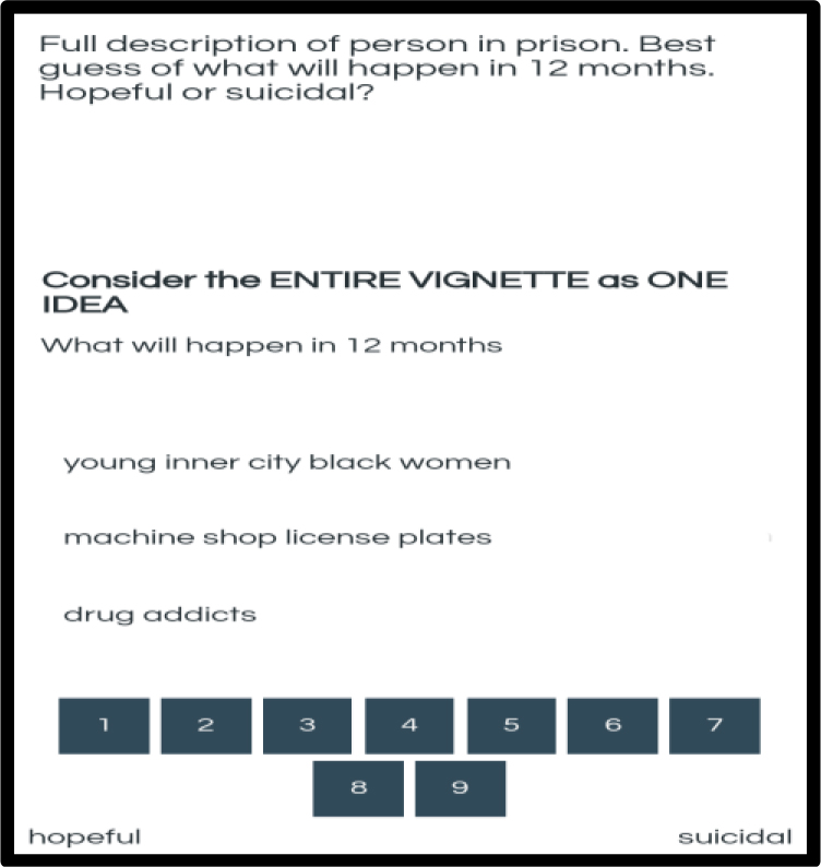
With the inputs shown in Table 1, Mind Genomics creates combinations of answers, so-called vignettes. An example of a vignette appears in (Figure 1).

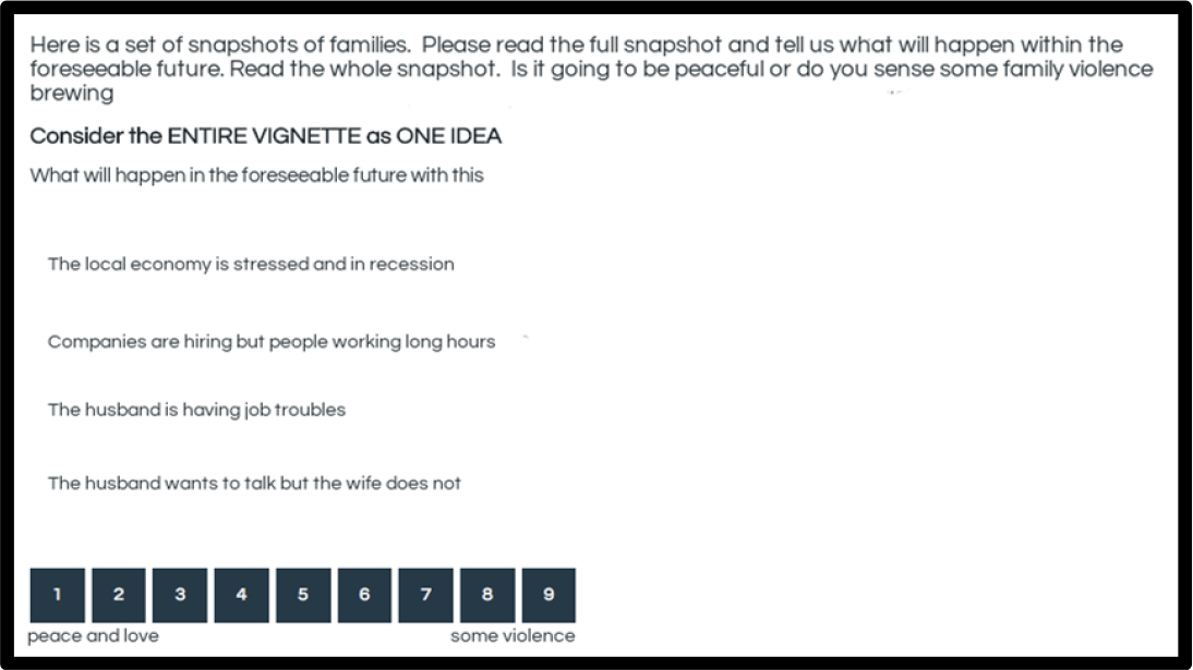
Figure 1. Example of a vignette as presented to the respondent.

Each respondent evaluated 24 vignettes. The vignettes were constructed according to an experimental design, with the property that a vignette comprised at most one answer from each question, but often had no answers from either one or two of the questions. Thus, the vignettes comprised either two, three, or four answers, the so-called elements. Furthermore, each respondent evaluated a unique set of combinations. The underlying structure of the combinations was maintained, but the specific combinations differed from one respondent to another. To the respondent, the combinations might seem to be random, but the reality is the exact opposite. The experimental design prescribes the combinations. The objective is to present combinations of elements or answers (without the questions), obtain ratings from the respondents who evaluate these combinations, and then deconstruct the ratings into the separate contribution from each element. In this way the respondent is unable to ‘game’ the system by providing politically correct answers. It is virtually impossible to detect the underlying pattern. As a result, the respondent simply relaxes, and gives responses which are more intuitive, and fundamentally less ‘edited.’ In the words of experimental psychologist Daniel Kahneman, the Mind Genomics approach calls into play ‘System 1’ thinking, the fast, almost automatic thinking that we use daily in our lives, when we don’t have to make rational calculations [10].

A sense of the underlying experimental design can be gotten from looking at the schematic in (Table 2), which presents the structure of the first eight vignettes for Respondent #1. The respondent does not, of course, see the underlying structure, but rather the actual combinations, presented on the computer as in Figure 1, or restructured to fit on the screen of a smartphone.

Table 2. Structure of the first eight vignettes for Respondent #1, the conversion to binary for statistical analysis, and the deconstruction of the ratings and response time.

Executing The Study

Each respondent receives the invitation to participate, and is instructed to read the vignette, and to rate it on the 9-point scale.

Here is a set of snapshots of families. Please read the full snapshot and tell us what will happen within the foreseeable future. Read the whole snapshot. Is it going to be peaceful or do you sense some family violence brewing?

What will happen in the foreseeable future with this family? 1 = peace and love … 9 = some violence

The respondent then read each of 24 unique vignettes. The respondent rated vignette on the above 9-point scale. The respondent was then instructed to fill out an open-ended question about violence (results not presented here.) The entire process took approximately 4–5 minutes.

Basic Data Transformation

The experimental design itself must be transformed to a binary no/yes, as shown in Table 2. Only with a binary scale (absent/present) is it feasible to understand the part-worth contribution of every element. In turn, the 9-point scale can be used as a dependent variable, but experience has shown that most people, researchers included, have a difficult time understanding what the scale points mean. Sometimes this difficulty in understand is addressed by labelling each of the nine scale points, a task which itself is fraught with difficulties. An easier way, taken from the world of consumer research, converts the nine-point scale to a binary scale, 0 or 100. Managers find it easy to understand the binary scale and know what to do with a ‘no’ or a ‘yes’ answer. The conventional way to divide the scale creates three regions for the scale; 1–3, 4–6, and 7–9, respectively. Then the following conventions is invoked:

Ratings of 7–9 are assumed to represent ‘violence, ’ and ratings 1–6 are assumed to reflect the lack of violence. For this new variable, ‘violence’, we convert ratings of 1–6 to 0, and ratings of 7–9 to 100. We then add a small random number (<10^–5.) The small random number ensures that that the regression analysis will ‘run’ on the binary-transformed data, even when the respondent confines all of the ratings either to the lower portion of the scale (1–6, transformed to 0), or confines all of the ratings to the upper portion of the scale (7–9 transformed to 100, 1–6 transformed to 0.) The small random number provides just enough variability in the dependent to ensure that the OLS (ordinary least = squares) regression ‘does not crash, ’

Analysis – what drives violence versus happiness – total panel?

The basic analysis in Mind Genomics is OLS (ordinary least-squares) regression, made possible by the ingoing structure of the vignettes for each individual respondent. Every respondent evaluated 24 carefully constructed vignettes, ensuring that at the individual level all 16 elements or answers to the questions, are statistically independent of each other. Most of the vignettes are different from each other, so that the combination of all the vignettes covers a great deal of the ‘design space.’ We combine all the data from the 50 respondents, creating a database of 1200 vignettes (50 x 24 = 1200.) We run two OLS regressions. The first relates the presence/absence of all 16 variables to the binary value of ‘violence’, corresponding to the ratings 7–9 on the original 9-point scale, but now becoming the value 100 on the binary scale for violence. The second OLS regression relates the presence/absence of all 16 variables to the violence of ‘happiness’ corresponding to the ratings of 1–3 on the original 9-point scale.

(Table 3) shows the coefficients for the two equations. The equation is expressed as (Binary Rating) = k₀ + k₁(A1) + k₂(A2) + … k₁₆(D4).

Table 3. Parameters of the model for the Total Panel relating the presence / absence of the 16 elements to predicted violence (Ratings of 7–9 converted to 100), and to predicted happiness (Ratings of 1–3 converted to 100.)

The additive constant, k₀, is the estimated value of the binary response in the absence of elements. All vignettes comprised a minimum of two and a maximum of four elements. Consequently, the additive constant is an estimated parameter. Nonetheless, the additive constant has value in because it gives a sense of baseline interest or baseline feeling, in the absence of elements. As noted above, the experimental designs ensure that all 16 elements or answers are statistically independent of each other, allowing the absolute coefficients to be estimated. That is, the values of the coefficients are all relative to 0. A coefficient of 10 is twice as high as a coefficient of 5. Furthermore, the transformation of the scale to binary strengthens the mathematic property. The coefficient of 10 means that in the absence of elements, 10% of the responses will be suggest ‘violence’ (7–9). The coefficient of 5 means that in the absence of elements, 5% of the responses, half the number as before, will suggest ‘violence.’ The absolute value of the coefficient means that the coefficients can be compared from study to study, with different topics and different respondents. The ratio scale properties generated by the binary transformation means that one can relate ratio changes in the coefficients (or properly coefficient + additive constant) to external behaviors. The negative coefficient means that when the element is added to the vignette, the percent of response suggesting ‘violence’ will be removed. Thus, when the coefficient is –10, then adding the element to a vignette will decrease the percent suggesting ‘violence’ by 10%. The coefficients are additive and subtractive.

From thousands of such experiments, a set of rules of thumb have emerged about the value of the coefficients, based upon observations of the data, and knowledge about what happens in the external world. The table below provides these guidelines, which are qualitative in nature. There are no fixed values, but rather a shading of importance, so that the higher the positive number the more important the element.

1.	Coefficient of 15 or higher	Extremely important, major signal
2.	Coefficient 8–15	Important to very important
3.	Coefficient of 0–8	From irrelevant to almost important
4.	Coefficient 0 to –6	From irrelevant to almost important
5.	Coefficient from –6 to lower	Important

We interpret the parameters of the model for violence (ratings of 7–9 converted to 100.)

1. The Additive constant is 27, meaning that there is a low likelihood of predicting violence in the absence of elements. We can compare this to say the purchase intent for pizza on the same type of 9-point scale, albeit with different anchors (definitely not buy … definitely buy). The additive constant for pizza is around 60.
2. The elements for predicted violence are low. There is only one which even approaches potential meaningfulness, C4 (The husband is sad and depressed).
3. We move now to the parameters of the model for happiness (ratings of 1–3 converted to 100.)
4. The additive constant is 12, meaning that there is very little in the way of predicted happiness in the absence of elements.
5. Two elements emerge as strong drivers of predicted happiness, both related to season:
   1. B4 (It’s summer time)
   2. B3 (It’s the middle of winter … Christmas)

Genders react differently when predicting violence, but similarly when predicting happiness

Respondents profiled themselves in term of gender. When we divide the data sets by gender and estimate the two models by gender (predicted violence versus predicted happiness), we find dramatic differences in the models for predicted violence, but similar models for predicted happiness (Table 4).

Table 4. Parameters of the model for males versus females relating the presence / absence of the 16 elements to predicted violence (Ratings of 7–9 converted to 100), and to predicted happiness (Ratings of 1–3 converted to 100.).

Predicted violence

1. Additive constant – lower for females, higher for males (16 vs 39.) The difference suggests that the prediction of violence by female respondent occurs for specific situations. In contrast, for males the additive constant is much higher, suggesting that they predict violence without needing to have specifics.
2. Women predict that the violence will occur in different situations, the most surprising of which is the expectation of violence during Christmas time.

   The husband is sad and depressed

   Companies are firing employees

   It’s in middle of winter … Christmas

Predicted happiness

1. Additive constant is very low, 11 for females, 13 for 13
2. Surprisingly, women are divided on winter and Christmas, with females reacting to

   It’s in the middle of winter … Christmas

   The local economy is growing

   It’s summer time

3. Males are happy as well, with both season and a growing economy

   It’s in the middle of winter … Christmas

   Companies are hiring but people are working long hours

   It’s summer time

When we move from gender to age, we see some dramatic differences as a person goes from older (age 50+) to younger (age 30 to 49, and then age 19 – 29.)

Predicted Violence

1. The additive constants, prediction of violence without other information, are low, with the additive constant lowest for age 50+ (value = 22), and the additive constant modestly higher for age 19 to 29 (value = 31)
2. There are age differences in what drives predicted violence.
3. The oldest respondents, age 50+ predict that violence will occur with the husband sad and depressed, and the companies firing employees.
4. The middle group age predict that violence will occur when the local economy is stressed and in recession
5. The young respondents don’t predict violence will occur in these bad economic times but predict violence will occur when the wife wants to talk but the husband does not.
6. We conclude from this pattern that the older respondents, age 50+, see violence as externally driven, whereas the young respondents, age 19–29 see violence as interaction driven.

Predicted happiness

1. The additive constants, base expectations without elements, vary dramatically across ages. The older respondents (age 50+ and age 30 to 49) see no basic happiness. It’s all a matter of the specifics. The younger respondents, age 19 to 29, in contrast, feel that happiness is all around.
2. The oldest respondents feel that happiness is a function of the time, whether Christmas or the summer.
3. The middle group, age 30 to 39, show some answers which make sense (e.g., companies are honoring, summer time, winter time), but also some answers which don’t make sense (companies are firing employees’ the local economy is stressed and in recession). It could be that this age group feels that the hard times will bring the couple together, rather than eventuate in violence.
4. The youngest group age 19 to 39 feel that happiness will emerge with the Christmas season, but not with the summer season (Table 5)

Table 5. Parameters of the model for the three age groups relating the presence / absence of the 16 elements to predicted violence (Ratings of 7–9 converted to 100), and to predicted happiness (Ratings of 1–3 converted to 100.).

Response time and engagement with the elements in the vignette

For more than a century, researchers have searched for ‘objective’ correlates of psychological processes. The notion that the information provided by people was not acceptable to many researchers, who believed, whether correctly or not, that only ‘objective’ physical measures could tell the truth about what a person perceives or thinks. The history of these approaches traces back to the original research on reaction time in the Leipzig laboratory of Wilhelm Wundt [11], and moves on to physiological measures of human reactions, whether GSR (galvanic skin response, electrical conductance of the skin), electromyography (muscle currents), then EEG (electroencephalographs and brain waves), culminating in such methods as fMRI [12, 13] There are other more recently introduced methods, such as the implicit association test [14].

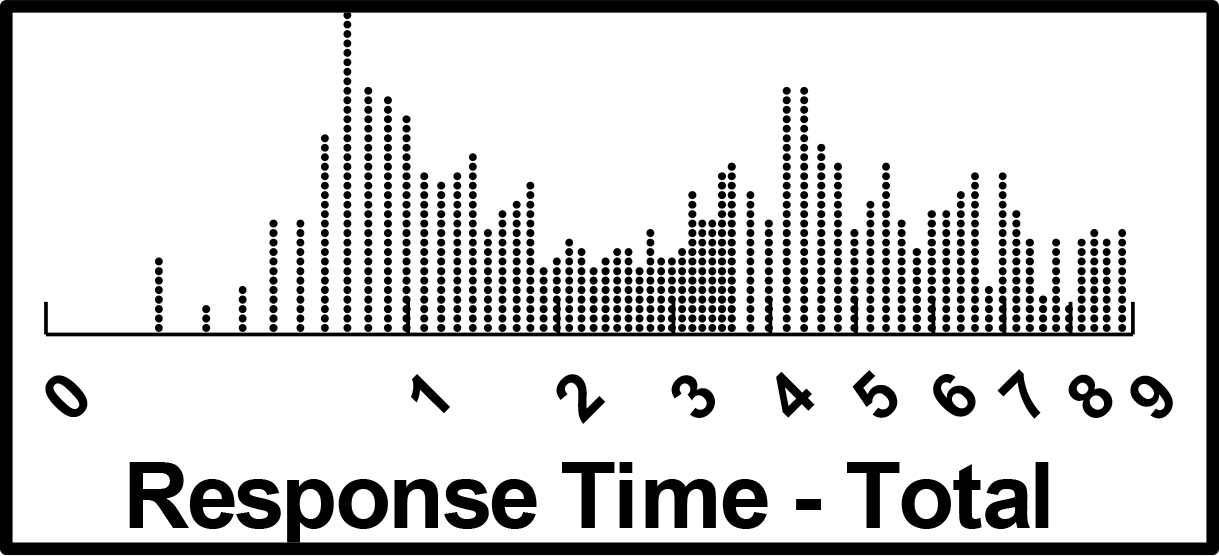
Response time, the earliest measure and perhaps the most frequently used measure, may shed additional light on the nature of the way people respond to the elements or answers embedded in the vignettes. Mind Genomics has the distinct benefit that the test stimuli, the elements, are themselves cognitively meaningful. It’s not a case of having to infer ‘what about the stimulus’ makes the respondent process it more quickly or more slowly. One can simply look at the response times to the different elements, using deconstruction method below, and ask whether there is something common about those elements taking longer to process, versus those elements processed more quickly. The Mind Genomics computer program measured the response time to the different vignettes. It then eliminated all vignettes requiring more than 9 seconds to rate, under the assumption that in these Mind Genomics studies, rarely does a respondent stop to consider a vignette for longer than a few seconds. The Mind Genomics program also eliminates all vignettes tested in the first position, with the rationale that at the start of the experiment respondents don’t know what to do.

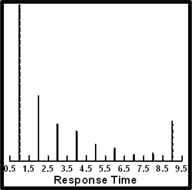
(Figure 2) shows the distribution of response times, with the abscissa spaced logarithmically. The important thing is the relatively large number of vignettes requiring more than four seconds to process. In many comparable studies, albeit with mundane topics like food, we do not see such long response times. There may be a difference in the way people read serious vignettes, such as the vignettes here, versus ‘fun vignettes’ of other topics.

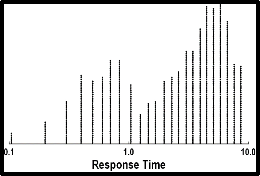
Figure 2. Distribution of response times for the study on predicted family violence. The distribution has been trimmed to eliminate the responses from the vignette evaluated in the first position, and vignettes registering 9 seconds or longer to evaluate.

The analysis of response times follows the standard approach, involving OLS (ordinary least-squares) regression. The equation is written without the additive constant, based upon the ingoing assumption that in the absence of a vignette with elements, there is no response. All vignettes, however, except those tested first, are included in the OLS regression, with all vignettes of response times 9 or more seconds truncated to 9.

The equation is expressed as: Response Time = k₁(A1) + k₂(A2) … k₁₆(D4)

The analysis was performed in the precisely the same way as the regression analyses for the ratings. That is, the relevant group was identified, and all the appropriate vignettes from everyone in the relevant group was put into a single data file, accessed by the OLS regression package. The coefficients represent the number of tenths of seconds that can be ascribed to each element. The OLS regression deconstructs the response time, estimating the number of tenths of seconds for each element. In the analyses we will look at those response times for individual elements of 1.5 seconds or more. The cut-off of 1.5 seconds is arbitrary, allowing us to get a sense of those elements which strongly engaged the respondents. It is important to keep in mind that these socially-relevant topics appear to be generating longer response times than the more typical business and marketing topics run in the same fashion, with the same type of respondents. It may be that respondents pay more attention to socially relevant topics

The response times for the 16 elements as shown in (Table 6) suggest a continuum with response times of 1.0–1.5 seconds. Keep in mind that all response times over 9 seconds or longer were eliminated as suggesting that the respondent might be doing other things. The data do not suggest a pattern. The most engaging elements, those with the longest response times, talk about the couple, about the economy, and about the woman having problems

Table 6. Response times for the 16 elements, estimated from the data of the Total Panel.

By gender

When we divide the respondents by gender, we see radical differences. The most important result is that men do not find the elements engaging, at least when we operationally define the term ‘engaging’ as a response time of 1.5 seconds (Table 7a).

Table 7a. Response times for the 16 elements, estimated from the data broken out by gender.

Males

The most engaging element is

            The lady is having problems with finances.

The least engaging elements are

            The wife wants to talk but the husband does not

            Companies are firing employees

            It’s summer time

            The family time is shorter together

            The husband is having job troubles

Females

There are many engaging elements. The fact that 8 of the 16 elements are engaging to women suggest that women are simply more attentive than men to the topic of violence versus happiness.

            The husband wants to talk but the wife does not

            The couple are having long term problems

            Companies are hiring but people working long hours

            The lady is having problems with finances

            The local economy is stressed and in recession

            The wife wants to talk but the husband does not

            It’s in middle of winter … Christmas

            Companies are firing employees

Age group

Respondents age 59+

The oldest respondents focus primarily about the issues between the members of the couple, but also react to the economy (companies are hiring but people working long hours.) That element might be a signal for problems that emerge between the husband and wife.

            Companies are hiring but people working long hours

            The husband wants to talk but the wife does not

            The couple are having long term problems

            The wife wants to talk but the husband does not

            The lady is having problems with finances

            It’s in middle of winter … Christmas

            Companies are firing employees

            The lady starts searching for a job to help out

Respondents age 30–49

The most engaging element is the practical issue of finances. The elements are more practical.

            The lady is having problems with finances

            The family all eat at different times

            The local economy is growing

Respondents age –29

None of the elements engaged them. They appear to be disinterested in the topic, or at least don’t pay much attention (Table 7b).

Table 7b. Response times for the 16 elements, estimated from the data broken out by age group.

Mind Sets

One of the key tenets of Mind Genomics is that in any topic area involving judgment and decision-making, there are different groups, mind-sets, showing divergent patterns of what is important. The ideal situation, but one quite rare, is that these mind-sets are congruent with some easy-to-define and measure characteristic or set of characteristics of the respondent. Most of psychological and sociological research discovering groups with different points of view, e.g., voting for political parties, attempt to understand these differences within the framework of the standard ways to divide people. Thus, it is not unusual to see voting patterns broken out by age, gender, market, income, education, work, and so forth. Indeed, the world of analytics attempts to predict these mind-set-driven behaviors from some predictive model using easy to measure variables. In the world of Mind Genomics, the discovery of these basic groups is straightforward, requiring simply one or several studies of the type performed here, and statistical methods to cluster together individuals with similar patterns of coefficients [15] Individuals with similar patterns are assumed to belong to the same ‘mind genome’ for the topic. The creation of the mind genome is a simple statistical analysis, once the relevant experiment has been run. In this respect Mind Genomics holds the advantage of generating easy to interpret ‘mind genomes’ from simple experiments. The reason for the simplicity is that the experiment deals with the topic itself, and the test stimuli are all relevant. One need not array an analytic armory to discover the ‘mind genomes, ’ which emerge readily from these focused experiments.

The procedure for uncovering mind genomes follows these eight steps.

1. Array the vector of all 16 elements for a given respondent as a one line in a data base.
2. Create all the data base, which in our case comprises 16 columns of data (one column per element), and 50 rows (one per respondent).
3. The coefficients tell us the degree to which the respondent would rate that element a 7–9 if the vignette comprised only that element.
4. Apply the method of clustering to divide the set of respondents into two groups, and then again into three groups.
5. Build a model for each of the two groups, and then build a model for each of the three groups.
6. Choose the more parsimonious solution, which is at the same time interpretable.
7. Interpretable means that the strongest positive elements ‘tell a coherent story’.
8. Parsimonious means that the fewer the number of clusters or mind-sets, the better, as long as the mind-sets tell a story which makes sense.

The results from the clustering suggest three mind-sets, as shown in (Table 8). The clustering was done on the coefficients after the ratings were converted to the ‘predicted violence scale’ (ratings of 7–9 converted to 100, ratings of 1–6 converted to 0.) The mind-sets are named according to the elements which generate the highest coefficients for the mind-set.

Table 8. Parameters of the model for the mind-sets relating the presence / absence of the 16 elements to predicted violence (Ratings of 7–9 converted to 100), and to predicted happiness (Ratings of 1–3 converted to 100.) The mind-sets were generated based upon the predicted violence scale.

When we look at response times for the three mind-sets (Table 9) we see dramatic differences in the pattern of elements which ‘engage, ’ i.e., operationally defined as generating a response time of 1.5 seconds or longer. The elements which drive the segmentation also appear to strongly engage only respondents in Mind-Set 3 (family has problems),

Table 9. Response times for the 16 elements, estimated from the separate models, one for each of the three mind-sets.

Mind-Set 3 (Family has problems)

            Companies are hiring but people working long hours

            The couple are having long term problems

            The lady is having problems with finances

            The husband wants to talk but the wife does not

            Companies are firing employees

            It’s in middle of winter are Christmas

Mind-Set 2 (Sensitive to the economy)

            The wife wants to talk but the husband does not

            The family all eat at different times

            The couple are having long term problems

            The local economy is stressed and in recession

            The husband wants to talk but the wife does not

            The local economy is growing

Mind-Set 1 (No specific warning)

            No element engages

The nature of people – optimistic versus pessimistic

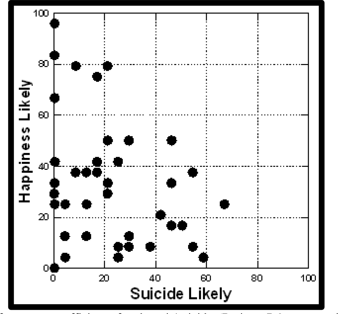
The original focus of this paper was the pattern of responses of people to vignettes describing a couple who are in a stressful situation. The pattern of responses of our 50 respondents can also show us whether the respondents themselves are typically optimistic, pessimistic, or neither. The analysis is straightforward. We have 24 samples of the respondent’s evaluations of vignettes, with all elements (answers) appearing an equal number of times, and the basic experimental design structure maintained.

In our preparation for modeling we created binary two scales, each 0/100. Each respondent generates an average on each binary scale. When we look at predicted violence, for example, an average of 100 means that 100% of the time, i.e., for all 24 vignettes, the respondent predicts violence will occur. In contrast, if the average if 50, then the respondent predicts that violence will occur on in half the vignettes.

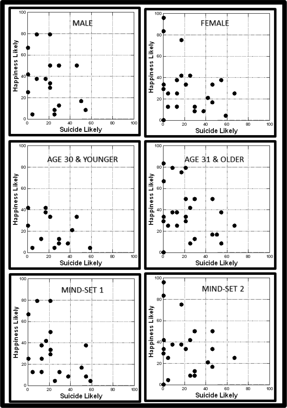
With this way of plotting the data we can look at the respondents, either one at a time or for key subgroups, to determine where the respondent lies on the scatterplot, and what that implies about the respondent. (Figure 3) shows the scatterplots for total panel, gender, age, and mind-set, respectively.

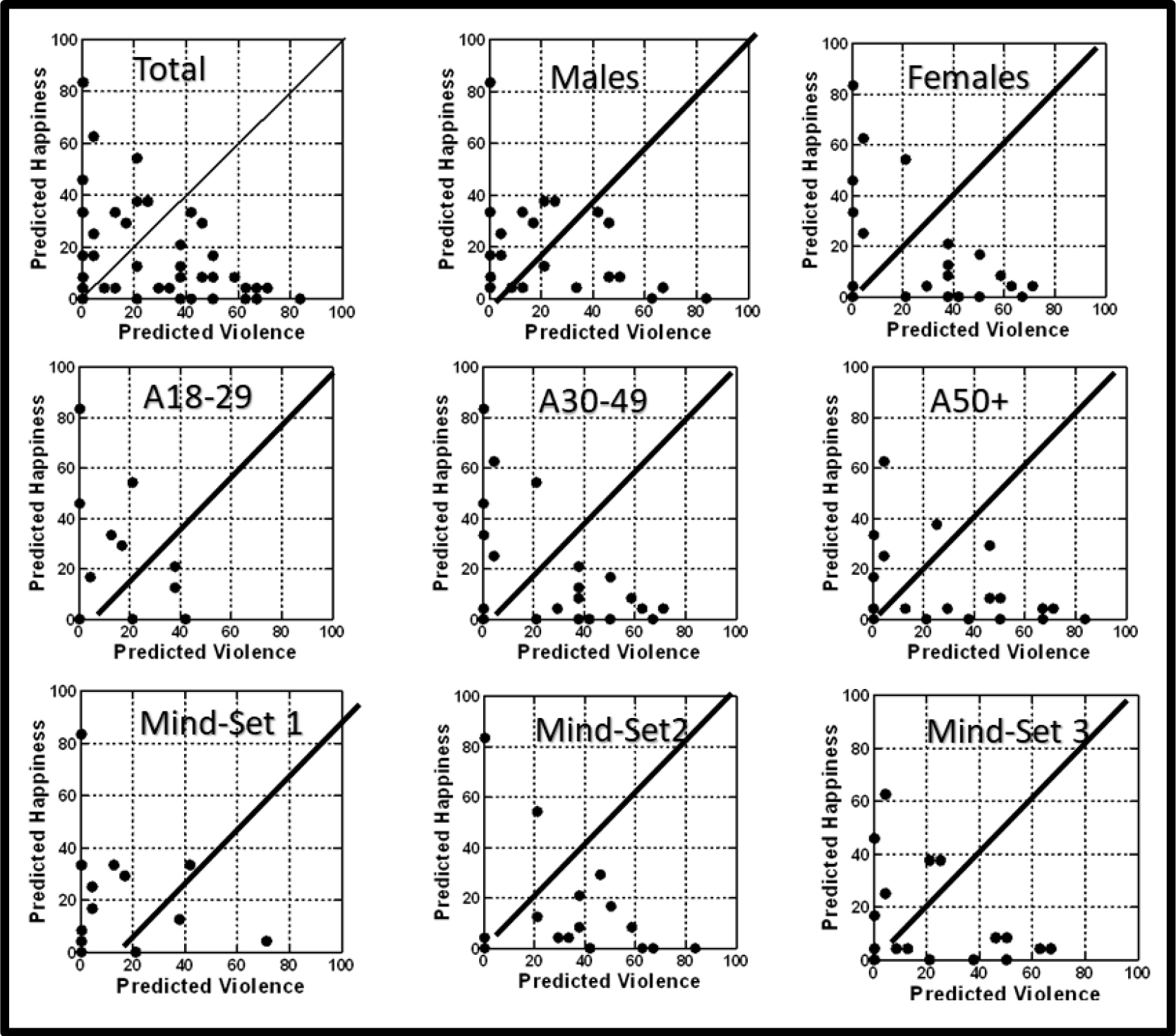
Figure 3. Scatterplot of binary transformed ratings. Each point is the average binary rating for a respondent. The abscissa is the average for the respondent for ‘predicted violence’ (rating 7–9 converted to 100.) The ordinate is the average for the respondent for ‘predicted happiness’ (rating of 1–3 converted to 100.)

The key things to note are:

1. The 45-degree line means that that the respondent is neither pessimistic nor optimistic but predicts violence and predicts happiness an equal number of times.
2. The further out on the abscissa and the ordinate the respondent falls, the more the respondent is judgmental. There respondent either rates the vignette as describing a situation ending in violence, or describing a situation ending in happiness.
3. The closer the respondent falls to 0, 0 the less frequently the respondent is judgmental.
4. Respondents falling to the right of the line and high on the abscissa (far right) tend to predict violence
5. Respondents falling above the line, and high on the abscissa (far up) tend to predict happiness.
6. Figure 3 immediately shows the greater negativity of females versus males, Age 50+ versus younger respondents, and Mind-Set 2 versus the other two mind-sets, respectively.

Finding the mind-sets in the population (Attila)

The conventional way to discover different groups in the population is through surveys. When one ‘knows’ the subgroup to which a person belongs, e.g., our mind-sets, it is only nature to believe that there are correlates of membership in the population. If only we could discover those correlates, goes the standard plaint. The ingoing assumption is that people who ‘think similarly’ (our mind-sets) should BE similar on the factors used to measure them. An example is age, another is gender, both of which, of course, are surrogates for various life situations and experiences.

(Table 10) suggests that if we are to look to age and to gender as co-variates of segment membership, we are likely to be disappointed. Certainly, as our data suggest, these subgroups exhibit their own general patterns, different from each other, but not suggesting profound differences. In contrast, mind-set segmentation of the type performed with Mind-Genomics data divides people by how they respond, and thus think, in a particular situation.

Table 10. Distribution of the respondents by both the mind-sets (columns) and the more traditional divisions (gender, age, respectively).

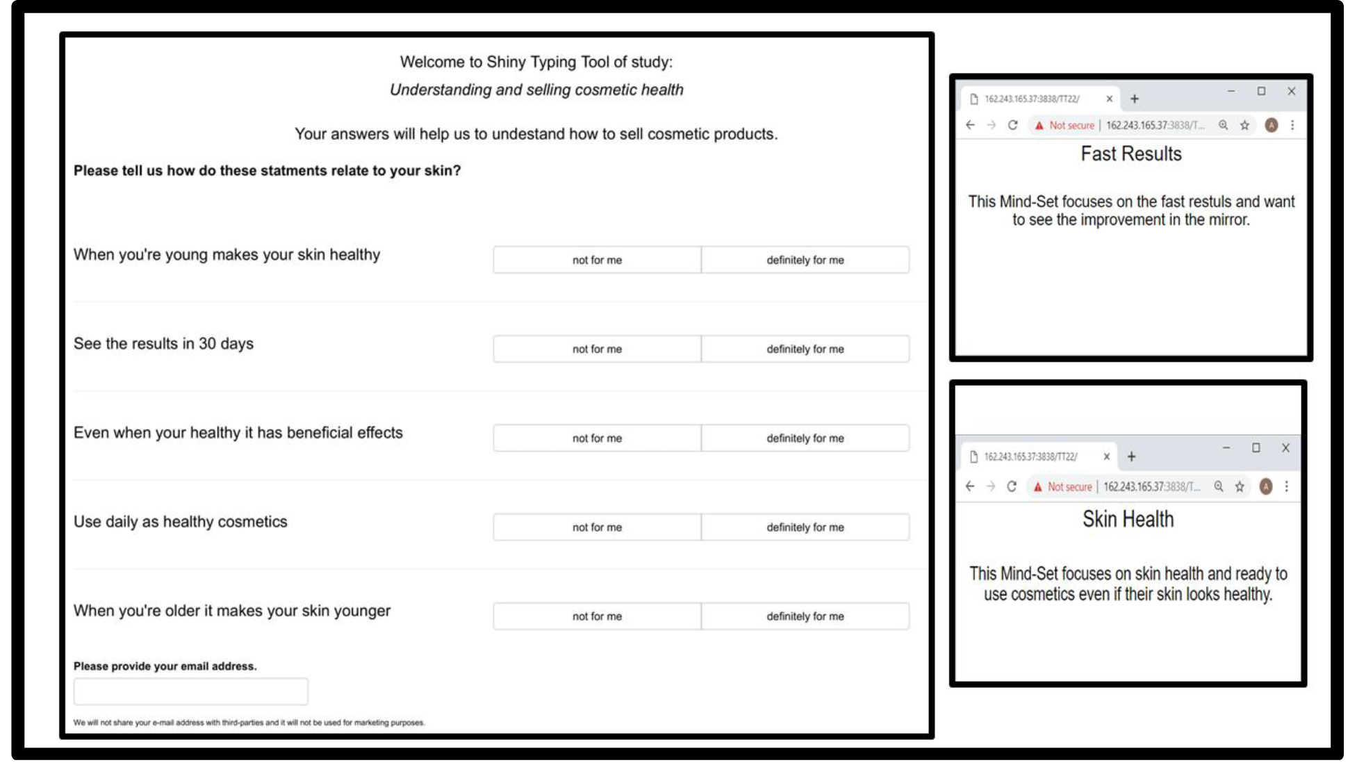
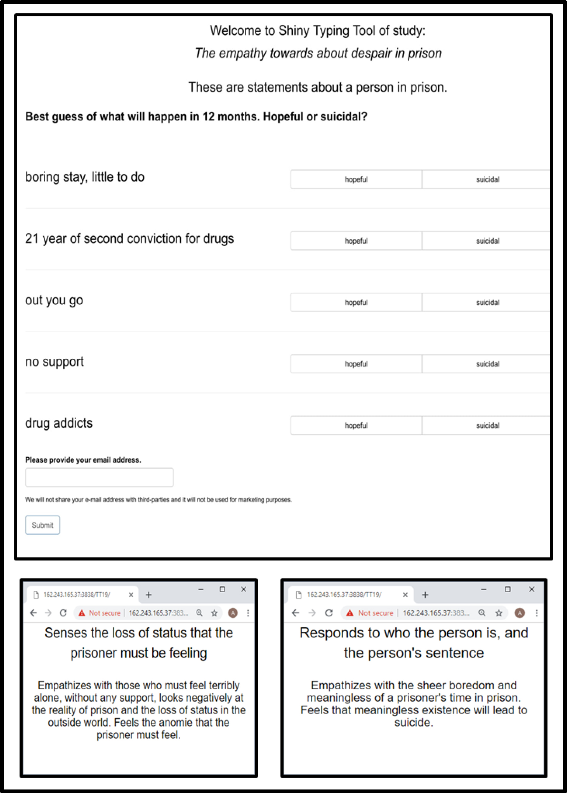
The specificity of the mind-set segments to the test stimuli means that we need a way to assign NEW people to one of the three mind-sets. The system must respect the fact that the mind-sets emerged from the elements specific to this topic and this study. Thus, we end up assigning new people to mind-sets based upon a system which is specific to the study. To this end, author Gere has created a PVI, personal viewpoint identifier which uses the pattern of coefficients from the averages for the three segments. The PVI is created by adding ‘noise’ to the basic summary data for the three mind-sets, and then using them to predict mind-set membership. The six strongest predictors in the ‘face of natural noise in data’ are selected as the cohort to be used to assign new people to one of the three mind-sets. (Figure 4) shows the PVI for this study, and the three feedback pages which emerge, depending upon the mind-set to which the respondent is assigned. The feedback pages can be used for further scientific study, for clinical purposes, and even for digital and personal marketing. As of this writing (March, 2019), the PVI is available this website:

Prediction of Violence: Violence: http://162.243.165.37:3838/TT20/

Prediction of Happiness: http://162.243.165.37:3838/TT21/

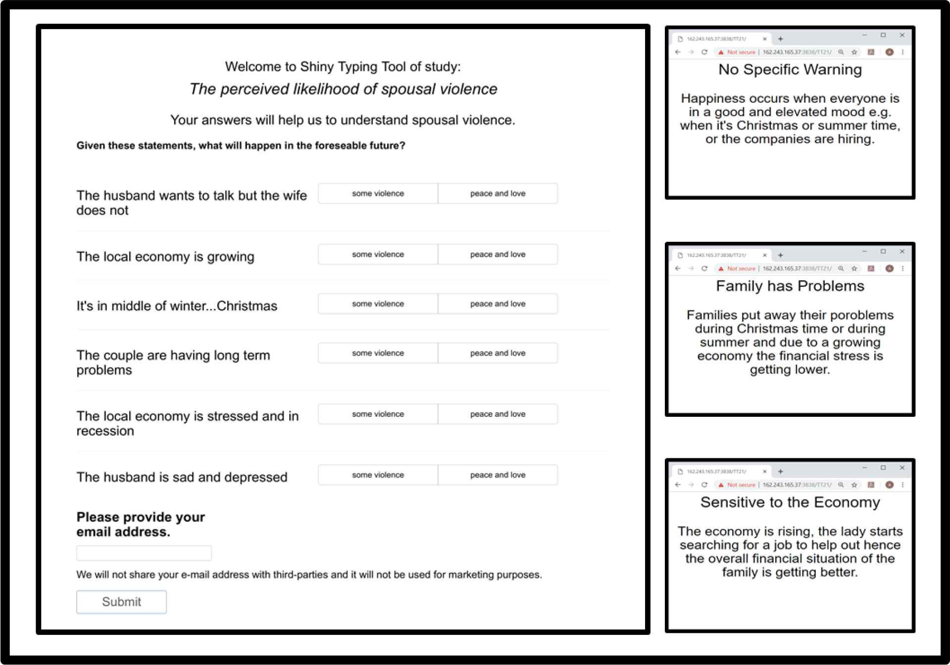
Figure 4. The PVI (personal viewpoint identifier) for the spousal violence study, by which new people can be assigned to one of the three mind-sets uncovered in the research.

Discussion and Conclusions

This paper presents the emerging science of Mind Genomics as a way to bridge the gap between the impersonal, quantitative dimension of social science and the qualitative, story-telling, emotion-filled and narrative-rich material provided by qualitative methods, story-telling, and literature.

The scientific literature dealing with marital violence provides us with a sense of the many different contributors to the violence in the home, mainly between spouses and but directed to other members of the family. There is a body of sociological and psychological data looking for correlates of family violence. The range of these correlated variables is extensive, as can be sensed from the small sample the literature cited here.

The problem with studying violence and other factors of the ‘human condition’ is the virtual impossibility of doing experiments. The ethics of science and the moral responsibility of people to act ethically precludes doing experiments. We are left with observations and reports. Mind Genomics steps in with an attempt to go one step further, using the ordinary individual as an observer of a reported situation (the experiment), and reacting in terms of a prediction of the outcome (violence, nothing, happiness, respectively.) In this respect we might consider Mind Genomics in these situations to be analogous to the behavioral economics tool of ‘predictive markets, ’ or better ‘information markets’ which uses subjective perceptions embedded in a stock market-like game to drive deep insights into the reasons behind choice [16].

The future holds the promise of learning such as we obtained here, not only for violence in the home, but literally for the many dozens, if not hundreds of life situations that do not permit of an experiment, but may yield some of their secrets to Mind Genomics, which combines the rigor of quantitative science with the richness of cognitively meaningful stimuli actually descriptive of normally lived lives.

Acknowledgment

Attila Gere thanks the support of Premium Postdoctoral Research Program of the Hungarian Academy of Sciences.

The authors wish to thank Dr. Gillie Gabay for her help in formulating the problem and placing it into its academic perspective.

References

1. Makepeace JM (1981) Courtship violence among college students. Family relations 97–102.
2. Poole C, Rietschlin J (2012) Intimate partner victimization among adults aged 60 and older: an analysis of the 1999 and 2004 General Social Survey. Journal of Elder Abuse & Neglect 24: 120–137.
3. Macmillan R, Gartner R (1999) When she brings home the bacon: Labor-force participation and the risk of spousal violence against women. Journal of Marriage and the Family 947–958.
4. Miller BA, Downs WR, Gondoli DM (1989) Spousal violence among alcoholic women as compared to a random household sample of women. Journal of Studies on Alcohol 50: 533–540.
5. Brinkerhoff MB, Grandin E, Lupri E (1992) Religious involvement and spousal violence: The Canadian case. Journal for the Scientific Study of Religion 15–31.
6. Dobash RP, Dobash RE, Wilson M, Daly M (1992) The myth of sexual symmetry in marital violence. Social problems 39: 71–91.
7. Fyfe JJ, Klinger DA, Flavin JM (1997) Differential police treatment of male-on-female spousal violence. Criminology 35: 455–473.
8. Stith SM, Farley SC (1993) A predictive model of male spousal violence. Journal of family violence 8: 183–201.
9. Moskowitz HR (2012) Mind genomics’: The experimental, inductive science of the ordinary, and its application to aspects of food and feeding’. Physiology & behavior 107: 606–613.
10. Kahneman D, Egan P (2011) Thinking, fast and slow. New York: Farrar, Straus and Giroux.
11. Blumenthal AL, Danziger K (2001) Wilhelm Wundt in history: The making of a scientific psychology. Springer Science & Business Media.
12. Nichols KA, Champness BG (1971) Eye gaze and the GSR. Journal of Experimental Social Psychology 7: 623–626.
13. Stipp H (2015) The Evolution of Neuromarketing Research: From Novelty to Mainstream: How Neuro Research Tools Improve Our Knowledge about Advertising. Journal of Advertising Research 55: 120–122.
14. Nosek BA, Greenwald AG, Banaji MR (2005) Understanding and using the Implicit Association Test: II. Method variables and construct validity. Personality and Social Psychology Bulletin 31: 166–180.
15. de Hoon MJ, Imoto S, Nolan J, Miyano S (2004) Open source clustering software. Bioinformatics 20: 1453–1454. [crossref]
16. Abramowicz M (2004) Information markets, administration decisionmaking, and predictive cost-benefit analysis. The university of Chicago Law Review 71: 933–1020.
17. Box GEP, Hunter WP, Hunter JS (1978) Statistics for experimenters, New York, John Wiley.
18. Gofman A, Moskowitz H (2010) Isomorphic permuted experimental designs and their application in conjoint analysis. Journal of Sensory Studies 25: 127–145.

DOI: 10.31038/ASMHS.2019322

Abstract

Prisoners are often thought to harbor thoughts about suicide, with sensationalized stories about the despair in prisons touching the hearts of listeners and readers. We explore the degree to which ordinary people, non-prisoners, feel that there is despair versus hope among prisoners. Through experimentally designed vignettes, we describe who the prisoner IS, what the prisoner FACES, what the OTHER PRISONERS are like, and what preparatory efforts are in place regarding RELEASE. Each respondent read a unique set of 24 vignettes, comprising different elements, and for each vignette rated the degree to which the prisoner would be likely to think of committing suicide versus be hopeful. The analysis reveals the specific contribution of each element in the vignette as a driver of projected suicide versus hopes, and the numbers of tenths of second required to ‘process’ the element before making the decision. The study suggests two mind-sets, one focusing on the prisoner, the other focusing on the surrounding, each as a driver of despair, as represented by the phrase ‘contemplates suicide.’

Introduction

The increasing cost of imprisonment, the increasing number of those imprisoned, and the alternative ways of imprisoning people, have created an entire industry of concern about what to do with the prisoner, how to rehabilitate the prisoner, and how to avoid post-release recidivism, or despair-driven suicide. Certainly, the prisoner, upon release, can be considered as a person with one or many ‘black marks, ’ responses by others to his or his misdeeds and punishments. The prospect of a life after prison or a life in prison, one marked with rejection and condemnation by society often leads to severe psychological and social problems. One of these is the possibility of contemplating suicide and then successfully suiciding. The recent literature, both popular and academic, deals with the emotions involved in prison.

The experience of imprisonment is difficult, with detrimental effects on prisoners and their families [1]. The nature of life in prison is particularly noticeable among women whose socialization left them with a lack of voice in the public domain. Female prisoners often referred to their feeling of helpless during their prison experience [2]

Accounts of prison life for males consistently describe a culture of mutual mistrust, fear, aggression and barely submerged violence [3]. Often too, prisoners adapt to this environment by putting on emotional ‘masks’ of masculine bravado hiding their vulnerabilities and deterring the aggression of their peers. Johnson [4] claimed that prisoners’ self-presentations of cool, hard manliness’ often reflect a ‘chronically defensive’ attitude rooted in feelings of moral self-doubt, social rejection and psychic vulnerability. This is a posture against the hurt that imprisonment threatens to expose [5]. Prisoners have a psychological need to re-establish their sense of masculine self-esteem and the need to develop personas to save them from exploitation [3]. De Viggiani [7] emphasized the ‘survival’ functions of prisoners whereas Jewkes [8] emphasized their jostling for positions of power in their depriving environments.

 Interviews with prisoners pointed to the protective functions of emotional self-control to hide fear or hurt which may be interpreted as signs of weakness exposing prisoners to ridicule and exploitation [3]. Prisoners expressed anger, fear, sadness and disgust through facial expressions [9] Emotional control is an internal defense as means of coping. Many prisoners stressed the need to control their emotions in order not avoid ‘cracking’ especially due to events outside the prison over which they had almost no control [3].

Occasional displays of emotion were deemed acceptable if they were the outcome of bereavements or if they related to children (e.g. serious illnesses, custody issues). Yet to unload one’s emotions on a continuing basis was reported to be unwelcome. In the visiting room, prisoners showed warmth and tenderness that were taboo on the landings, closed to visitors. Visits offered the only opportunity to display authentic feelings and to show warmth. Some were visibly upset as their visitors left, or sat in silent contemplation, their stolidity contrasting with the animated tone of a few minutes earlier.

Although there are many studies about the statistics of prisoners and imprisonment, along with interview accounts with prisoners, there is relatively little in the literature about metric studies on the ‘mind’ of the prisoner from the point of view of those who are not prisoners, i.e., studies of one’s empathic feeling toward prisoners. This study examines the perception of the public regarding emotions of prisoners and the extent of empathy understanding, with empathy being the ability to ‘sense the feeling of the other. This paper introduces a new approach to thinking about a topic, namely the study of empathy of normal people towards people who find themselves in a particularly stressful situation. The worlds of literature and song, stories, novels, poems, ballads, are is filled with descriptions of how one person feels about another or a group of others. Science is not, however, at least with descriptions having depth and tonality. This study begins that new course of research effort.

Method

Mind Genomics is an emerging science of the ‘everyday, ’ studying how people make decisions when confront by descriptions of ordinary experience, or at least experiences which could happen to people, experiences with which people are familiar [10, 11] Mind Genomics moves away from the traditional scientific approach of isolating one variable at a time and studying that variables. Rather, the premise of Mind Genomics is that we are continually confronted by compound situations, comprising many aspects. We, ordinary people, seem to have no trouble coping with these compound situations, making a series of decisions, and moving forward. Often, we are not able to articulate the reason WHY we do what we do. Yet, our behavior is rapid, automatic, appearing considered rather than random.

In its world-view and execution, Mind Genomics differs from most conventional research, which pay a great attention to the test stimuli, and may test a very few stimuli, but offer a variety of conclusions and implications from one study. With Mind Genomics, we look at simple, broad brush strokes of different aspects of prison, and do fast, simple research. Our metaphor is to cover ground, to explore, much like a cartographer explores and maps out an area, without paying very close attention to the minutiae of the area being mapped. The goal is to understand the key points of the topic, what ideas drive strong responses, what ideas drive strong engagements. The responses are measured using rating scales, converted later to a binary scale. The engagements are measured by response time, deconstructed into the number of tenths of second a statement ‘holds the respondent’s attention’ while being processed.

The test stimuli comprise four questions dealing with the person who is in prison, what the person does basis, the nature of other people in the prison, and the preparations, if any, for re-entry. The four questions are used as prompts to drive the researcher to provide four answers to each question. Table 1 show the four questions and the four answers to each question.

Table 1. The four questions, and the four answers to each question.

Test stimuli created by experimental design

The typical way to understand what people feel about a topic is to ask them questions about the topic, either in discussion (interviews), or through a survey on pencil and paper. An emerging way to understand people is the belief that observing their recorded behavior, e.g., what the person buys or does, gives a sense of who the person is, and what the person believes. This latter approach, is called ‘Big Data.’ The reality is that each of the approaches provides some information about the person, but does not provide the specific information for the topic. Our topic is the empathy of normal people towards their ideas of prisoners, and specifically prisoner despair. There is no way that Big Data can provide this information. Rarely can we find a survey which focuses on this topic because the topic is so specific, and so different from the more mainstream, conventional topics in the world of sociological or psychological research,

Mind Genomics approaches the issue of empathy about prisoner despair by running a simple experiment. The respondent or subject is provided with test combination of the 16 answers, and instructed to rate the combination, the vignette, on an anchored 9-point scale, with the scale focusing on an assessment of estimated feelings. Figure 1 shows the test stimulus.

Figure 1. Example of a 3-element vignette about a prisoner, and the instruction to the respondent to rate.

The underlying experimental design comprises a ‘recipe’ or systematic layout of 24 combinations, vignettes, each vignette comprising 2–4 elements or answers, selected from Table 1. Each respondent evaluated 24 different vignettes, comprising 2–4 elements per vignette, at most one element or answer from one question. The experimental design presents the combinations without concern as to whether the combination ‘makes sense’ [12] The objective is to present the respondent with a set of test stimuli and force a judgment, that judgment being a rating of the entire vignette. The respondent cannot assign a ‘politically correct rating’ because there is no underlying pattern that the respondent can discern. The respondent may begin by trying to be politically correct and do the task ‘properly’ by paying attention, but soon gets frustrated, and reacts at an almost automatic, intuitive, ‘gut level.’ This is the desired state for the respondent. The intuitive response means that the response will be relatively uncontaminated by what the respondent feels to be that which the research ‘wants.’

The experiment with 42 respondents generated a data set, comprising 1208 vignettes. Most of the vignettes differed from one another. This structure of testing different combinations by each respondent is known as a permutable experimental design [13] The structure allows the researcher to ‘cover the space’ of possible test combinations, an approach analogous to the MRI (taking different pictures of the tissue), rather than the way typical scientific research works (repeating the pictures many times to reduce the error of measurement.)

Analysis

The ratings from the respondents were transformed to a binary scale, following the approach used by author HRM for 35 years, since the mid 1980’s, and based upon a combination of experience and common industry practice. Experience suggests that most users of scales do not know what the scales mean. Often the user of the data, the ultimate ‘client’ of the results, asks for an interpretation, such as ‘is a 6 a lot or a little better than a 5, or a little or a lot worse than a 7?’ These questions continue to reaffirm the fact that the user of the data does not really understand what to do with the data, other than to make conclusions about ‘better or worse.’ A more productive approach, used for decades by market researchers bifurcates the scale, so that there is a top of the scale (e.g., 7–9), and a bottom of the scale (e.g., 1–6). In our case, we would interpret the top of the scale, the ratings of 7–9, as indicating that the prisoner is believed to be thinking of suicide. A rating of 1–6 indicates that the prison is not likely to commit suicide, or to think about committing suicide. We can also look at the scale from the opposite end, hopefulness with a rating of 1–3 indicating that the prisoner is believed to be hopeful,

The underlying experimental design enables us to combine the data from our 42 respondents into a database comprising the 1008 observation. Each observation comes from one respondent, one vignette. The experimental design ensures that the 16 predictor variables, the elements, are statistically independent of each other. The dependent is augmented by the addition of a very small random number, approximately 10^–5

Table 2 shows the results from the first OLS (ordinary least-squares) regression, focusing on the data from the transformation to the binary scale (1–6 = not thinking about suicide; 7–9 = thinking about suicide.) The regression procedure, colloquially known as curve fitting, deconstructs the 0/100 binary rating into the basic contribution of the 16 elements, the 16 coefficients, and an estimated basic level, the additive constant.

Table 2. Coefficients for ‘thinking about suicide’ (ratings 7–9 converted to binary). Data from the total panel.

The interpretation of the results is straightforward:

1. The additive constant is the estimated probability of a respondent saying that the person described in the vignette will attempt suicide (rating 7–9 on the scale.) The additive constant is 24.46, which we interpret to mean that in the absence of elements, the expected proportion of responses 7–9 (thinking of suicide) is 24.46, about 25%.
2. Table 2 shows the 16 elements sorted from highest (believed most likely to think of suicide), to lowest (believed least likely think of suicide.)
3. The coefficients have ratio-scale values, so that a value of 10 means believed twice as likely to thinking of suicide than a value of 5.
4. The coefficients can be added to the additive constant to create a sum which provides the estimated probability of a prisoner thinking about suicide. Thus, one needs only the additive constant, and the elements, as well as their coefficients, to estimate the likelihood that one believes that thoughts of suicide will plague prisoner described by the vignette.
5. The coefficients in Table 2 suggest that the two elements co-varying most strongly with likelihood of suicide are C3 (drug addicts, as fellow prisoners), and D3 (the recognition of no support.) These two elements talk about two aspects, one who the fellow prisoners happen to be, and second the emotional support in the prison.
6. The coefficients suggest that two descriptions are least likely to covary with the thought of suicide. One is the young inner-city black woman, the other is optional courses to prepare for jobs. These are radically different. The first suggests the appreciation who the prisoner happens to be. The second is the fact that someone is taking care of the prisoner, or at least thinking of the prison to prepare for a job.
7. The T statistics tells us the ratio of the coefficient to the standard error of the coefficient. The higher the T statistic, the more likely it is that the coefficient or the additive constant comes from a distribution whose true value is not 0. The P value, in turn, is the probability that the T statistic comes from a distribution whose true value is 0.

Reversing the perspective – what drives the rating of ‘hopeful’ (1–3 on the 9-point scale)

Our respondents could assign rights on either side of the scale, 1 representing hopeful, 9 representing contemplating suicide at some point. What happens when we focus on the positive aspects, looking at the elements driving the ratings of 1–3. We now convert the ratings on the low end of the scale, 1–3, corresponding to hopeful, so that they become. In turn, the value 100. The remaining six scale points, 4–9, become 0, to denote not hopeful. We perform the same analysis on the data from the total panel, looking at the additive constant, and the coefficient for each element.

1. The additive constant is 43.79, almost 44, meaning that in the absence of elements, almost half of the responses will be between 1 and 3, hopeful. We interpret this to mean that it is basic information (a person is in prison) which conveys some hope. Being in prison does not automatically drive one’s feeling that the imprisoned person will contemplate suicide. Being is prison does, however, drive a sense that the prisoner will be modestly hopeful.
2. Estimated hopefulness is driven by reading about preparations for release, such as ‘optional courses to prepare for job’, and ‘4-hours of forced library.’.
3. Lack of hopefulness is driven by who a person is, and the situation in the prison. These are the elements with the lowest coefficients for hopefulness.

   21-year-old second conviction for drugs

   54-year-old woman convicted for drugs

   drug addicts (in prison)

   white middle age for theft

   no support

Individuals – are they optimistic or pessimistic, based upon their coefficients

Can we classify an individual as optimistic (perceiving the situations in the vignette as ‘hopeful’) or pessimistic (contemplating suicide), both or neither? One way to answer this question computes the average coefficient across 16 elements for each individual, when we look at the equation for ratings of 7–9. Recall that the coefficient shows the believed likelihood that the prisoner being described is likely to commit suicide. Each respondent generates 16 coefficients. The average coefficient for a respondent tells us the proclivity of the respondent to see the described prisoner’s feelings as leading to thoughts of suicide. The second part of the answer is to compute the average for the same respondents for the 16 coefficients dealing with hopeful. The average coefficient for a respondent tells us the proclivity of the respondent to see the described prisoner vignette as leading to hopefulness.

We begin with the scattergram for the total panel, in Figure 2. Each filled point represents one respondent. The abscissa corresponds to the average of the respondent’s 16 coefficients on the top part of the scale, tendency to suicide, i.e., the coefficients of the individual-level regression model run for the respondents when the ratings of 1–6 were converted to 0, and the ratings of 7–9 were converted to 100. The ordinate corresponds to the average of the respondent’s 16 coefficients on the bottom of the scale, hopeful, when the ratings of 1–3 were converted to 100, and the ratings of 4–9 were converted to 0.

Figure 2. Distribution of average coefficients for despair/suicide (Ratings 7–9 converted to binary) and average coefficients for happiness/hopefulness (Ratings 1–3 converted to binary). Each filled circle corresponds to a respondent.

When the respondent cluster at 0, 0, we conclude that the respondent does not sense either prisoner despair or prisoner hopefulness in the vignettes. The averages for the latter two scales are both near 0, and thus the respondent falls at the bottom left. The further out to the right on the abscissa lies the respondent’s average, the more the respondent feels that the prisoner will contemplate suicide. The further up the ordinate lies respondent’s average more the respondent feels that the prisoner will feel hopeful. Figure 2 suggests more respondents feel that the prisoner will be hopeful, and fewer respondents will feel that the prisoner will contemplate suicide. Looking more closely at the distribution, we see about five respondents who feel primarily despair in the vignettes, and about five respondents who feel primarily hopefulness in the vignettes.

As a side note, this format of presenting data suggests a new way to understand the basic mind-set of a person on two opposing dimensions of a feeling. The location of the points gives a sense of how different people think and empathize. Most of the respondents in the large area between 0, 0 and 0.3, 0.3. The location 0, 0 corresponds to a person who is neither pessimistic nor optimistic in the estimation of how the prisoner would feel. The location 0.5, 0.5 corresponds to the location where the person is absolutely decisive, rating the vignettes as either hopeful or despairing (contemplate suicide.) For the person located at 0.5, 0.5, there is no middle ground. For the person located at 0, 0 there is virtually only middle ground.

Subgroups – Gender, Age, Mind-Set – What is expected to drive the prisoner’s though to suicide?

One of the key benefits of the Mind Genomics approach is the use of different combinations of vignettes for each respondent, but at the same time ensure that each respondent evaluates the appropriate set of vignettes in order to create an experimental design. One can do the analysis on key subgroups, both self-defined (gender, age), and defined through analysis (mind-set.) The small group of 42 respondents provides sufficient depth into the mind of the respondent to reveal the responses of subgroups, perhaps a bit noisily, but nonetheless powerfully.

Table 4 shows the set of key subgroups. For this study we divided the respondents by gender and by age, respectively, and then created mind-set segments as described in the following section.

Table 3. Coefficients for ‘hopeful’ (ratings 1–3 converted to binary). Data from the total panel.

Table 4. Strongest performing elements by key subgroup of the models relating the presence/absence of elements to the estimate of the prisoner’s contemplation of suicide.

1. Additive constant – all subgroups are approximately the same, showing an additive constant of 22 – 27.
2. Males feel that simply ‘being bored, having nothing to do’ is a cause for contemplating suicide. Females do not.
3. There is no difference in projected potential of contemplating suicide by younger versus older respondent.
4. We created two mind-sets by clustering the array of 16 coefficients, and extracting two different groups, which are maximally different from each other (De Hoon et. al., 2004.) Clustering is a purely statistical technique. We extract the fewest number of clusters (parsimony) which tell coherent stories (interpretability.)
5. Mind-Set 1 feels that the prisoner will think of suicide if there is no emotional support in the prison, and if the prisoner is simply discharged, released, without any preparation. To Mind-Set 1, it is the sense of aloneness in the prisoner which is distressing. Mind-Set 1 can be called ‘want preparation.’
6. Mind-Set 2 feels that the prisoner will contemplate suicide if there is a sense of nothing to do, and if the prisoner is either a serious drug addict (second conviction) or surround by drug addicts. Mind-Set 2 can be called sensitive to surroundings.

Subgroups – Gender, Age, Mind-Set – What is expected to drive the prisoner’s thoughts to happy

We can follow the same logic, this time looking at gender, age, and newly constructed mind-sets for the low part of the scale, ‘hopeful.’

1. Males show a much higher imputed basic hopefulness for prisoners than do females (54 versus 36.) Without any additional information, males believe that that the prisoner will be neither hopeful or not hopeful (additive constant 54), whereas females believe that it’s more likely that the prisoner will not be hopeful (additive constant 36).
2. For males, hopeful is perceived as a matter of preparing for a job and being surrounded by prisoners who are middle class.
3. For females, hopefulness is perceived when the message is about preparing for a job, library, rehabilitation, and surprisingly, with the prisoner has little to do. Males, in contrast feel when the prisoner in bored, and has little to do, the despair is higher, with a greater thought of suicide.
4. Younger respondents (under 30) feel that hopefulness will come from job preparation and from the hours in the library.
5. Older people feel the same way, and also feel that hopefulness will come from being surrounded by middle class prisoners.
6. The previously created Mind Set 1 feels that hopefulness is a matter of the requirement of four forced hours in library, as well as being surround by middle-class prisoners.
7. The previously created Mind-Set 2 feels that hopefulness will come with the preparatory course for jobs, and the requirement of library.

Subgroups – are they optimistic or pessimistic, based upon their coefficients

The previous analysis for the total panel presented a novel way to gauge whether the respondents are optimistic or pessimistic, by plotting the average coefficient from the two models, doing so for each respondent. The coefficient shows the average conditional probability that the respondent would assign the element a rating of 7–9 (top 3, contemplating suicide), versus that the same respondent would assign the element of 1–3 (bottom 3, happy). The two averages come from the coefficients of 16 elements.

When we plot each respondent on a two-dimensional graph, we can sense the respondent’s mind. To review:

1. Each filled circle corresponds to one respondent
2. The location 0, 0 corresponds to a person who is ‘all middle ground, ’ sensing neither despair leading to contemplation of suicide, nor sensing hopefulness. All the ratings for the vignettes lie between 4 and 6.
3. The location 0.5, 0.5 corresponds to a person for whom there is ‘no middle ground’ but not basically optimistic nor basically pessimistic in the estimation of how a prisoner would feel.
4. Plots to the right on the abscissa suggest a person who is more pessimistic, and sees despair leading to the contemplation of suicide.
5. Plots upwards on the ordinate suggest a person who is more optimistic, and sees ‘hopefulness’

Figure 3 shows the plots for key subgroups. Each panel (top,
middle, bottom) compares two complementary subgroups. The
statements below are purely from visual observation and impression,
not from a statistical analysis.

Figure 3. Distribution of average coefficients for despair/suicide (Ratings 7–9 converted to binary) and average coefficients for happiness/hopefulness (Ratings 1–3 converted to binary). Each filled circle corresponds to a respondent. The three panels show the results for complementary subgroups.

1. Females show more respondents closer to the 45-degree line, and further out than men on that line. Qualitatively, females seem to be more judgmental than men, but neither overly optimistic nor pessimistic.
2. Younger respondents aged 30 and younger show more respondents lying close to the non-judgmental region of 0, 0. Older respondents age 31 and older show more respondents as lying further out towards 0.5, 0.5, with a tendency to be more optimistic, and feeling that the prisoner is more hopeful.
3. Mind-Set 1 (want preparation) appears to be less judgmental, and if judgmental then optimistic in terms of rating what the prisoner would feel. Mind-Set 2 (sensitive to surroundings) is more judgmental, with fewer ratings in the 4–6 region of the scale. Mind-Set 2 appears to be slightly more pessimistic.

Response Time

The previous sections dealt with the analysis of the ratings, specifically what elements are perceived, in one’s opinion to correlate with thinking that would contemplate suicide, at least in the opinion of a non-prisoner respondent reading a vignette about the prisoner. The analysis deals with the conscious assignment of ratings to the test stimuli, even if the decisions tend to be automatic.

Researchers have been interested in the past few years in possibly deeper mechanisms of decision-making, many of which they put in the grab-bag called neuromarketing, or more correctly non-conscious, physiological correlates of decision-making. Fugate [15], Lee et. al. [16] and Stipp [17] summarize this new area of neuromarketing, or really physiological correlates of messaging. Genco et. al. [18] have popularized in a book ‘Neuromarketing for Dummies.’ We now proceed to the analysis of one of one of these measures, response time. The ingoing assumption is that longer response times signal that the respondent is somehow ‘engaged’ in reading and thinking about the particular element in the vignette.

Some of the vignettes constructed were responded to slowly, others were responded to quickly. After removing the first vignette evaluated by each respondent because the respondent was just ‘learning what to do in the experiment, ’ and after removing all vignettes responded to after 9 seconds because it was likely the respondent was doing something else, we emerge with a distribution of response times as shown in Figure 4. The time scale, abscissa, is logarithmically spaced, emphasizing the many vignettes responded to faster than 2 seconds. The computer program picked up the response times in tenths of seconds.

Figure 4. Distribution of the response times for the vignettes, after removal of the first vignette and after removal of all response times of 9 seconds or longer.

As stated above, we assume response time to be a correlate of engagement. We operationally define the term as ‘time spent attributed to the element when the vignette is being evaluated.’ We cannot, of course, ask the respondent to tell us how engaging each element seems to be, although occasionally the novice researcher might ask that question. The reading and response occur so rapidly, so automatically, that the respondents are not aware of what holds their attention unless there is something so powerfully strong that it ‘stops’ the respondent.

The experimental design enables us to estimate the likely number of seconds in the response time that can be attributed to each element. It is important to note that this assignment is an estimate, only, based upon the application of OLS regression to the response times. Some interesting patterns emerge from Table 5.

The elements are presented in descending order of response time based upon the results from the total panel. These ratings are from 40 respondents, each evaluating at most 23 vignettes, but a number of vignettes have been removed because they were recorded as being unusually long.

We have highlighted and bolded those response times of 1.4 seconds or longer, which can be assumed to be ‘engaging.’ The choice of 1.4 seconds is simply to represent a time that can be thought of as possibly conscious attention.

The longest response time for any group is 1.7 seconds (female respondents with the element ‘lower and upper middle class’).

The shortest response time for any group is virtually 0 time, ‘optional courses to prepare for jobs’ (0.2 seconds, for Mind-Set 2, who are sensitive to their surroundings, and would be expected not to care about courses for the future.)

Total panel: The longest response times, i.e., the most engaging, are descriptions of the person, requiring multiple words. The shortest times, i.e., the least engaging, are descriptions of occupation training in prison. It’s all about the people, who they are.

Assigning new individuals to one of the two mind-sets

Conventional research is grounded on the belief that there is an indivisible link between who the person IS and what the person THINKS. This belief motivates the use of large, representative samples of respondents, believing that it is important to measure the correct group of people in order to understand the way the mind works. Thus, good practice in business and political polling is often accompanied by large base sizes and a measure of ‘error, ’ or underlying variability.

Table 5. Strongest performing elements by key subgroup of the models relating the presence/absence of elements to the estimate of the prisoner’s hopefulness.

Table 6. Coefficients for response times, by total panel and key subgroups. Coefficients of 1.4 or higher are shown in shaded cells, with bold numbers.

One of the premises of Mind Genomics is that in virtually any topic area where human judgment comes into play one can discover different points of view, different criteria for judgment. These are called Mind-Sets. Their reality emerges from the analysis of how individuals respond to the different elements or ‘answers’ in the particular study. That is, these mind-sets exist, but are really groups of individuals who behave similarly in a specific situation, as revealed by their patterns of responses, or perhaps as the next paragraph suggests, mind-sets are really combinations of ideas.

Underlying the research in Mind Genomics is the belief that some ideas ‘flow together.’ It is the combination of such ideas which flow together that comprises the focus of interest of Mind Genomics. Individuals, the respondents who participate, are ‘protoplasm’ which in some way embody these basic mind-sets, but the individuals are NOT the mind-sets. The mind-sets are primaries, like the colors red, yellow and blue. Each person comprises a set of mind-sets, with the methods of Mind Genomics both identifying the nature of the mind-sets from clustering, and establishing who in a study embodies each mind-set. Whether these mind-sets represent true primaries like color primaries, red, blue and yellow, is not important. What is important is that they show remarkably different, and interpretable patterns of responses, patterns which make sense, can be interpreted and labelled. These primaries may co-vary with external behaviors, and perhaps even with physiological patterns of responses. What is important is that they represent a new way of looking at individual differences.

With the foregoing accepted, the question is whether there is a natural affinity for the mind-sets established in an experiment to distribute in the way to which we have been accustomed. That is, for our study we have established two mind-sets, those who want preparation, and those who are sensitive to their surroundings, etc.

Table 7 shows that there is no clear relation between mind-set membership and either gender or age. This is typically the case. Mind-sets emerge quite clearly in Mind Genomics studies, but these mind-sets do not distribute in ways that are easy to discern, despite the radical differences in content between or among the mind-sets.

Table 7. Distribution of the two mind-sets by gender and age, respectively.

Given the clear similarity in the patterns of WHO are in the two mind-sets, at least in terms of gender and age, how then do we assign a new person to a mind-set? This is an important question, both for science, and for commerce. For science, we can begin to study the relation between membership in a mind-set for one topic, and both membership in other mind-sets for other topics, and/or external behaviors, and even biological/genetic covariates of membership in different mind-sets.

Our approach uses the average coefficients from each mind-set. We create 1, 000 different variations of the average profile by adding ‘noise’ to the coefficients. We then identify the six questions which, in the presence of “noise” can be used to correctly assign the respondents to the correct mind-set. Figure 5 shows an example of the PVI (personal viewpoint identifier), presenting the six strongest questions which, in concert, help us assign a person to the correct mind-set. We also show the feedback page, which can go to the person being typed, or be used to drive the respondent to the right e-commerce website, or perhaps incorporated into the person’s profile for future use. As of this writing (March, 2019), the PVI is located at this location: http://162.243.165.37:3838/TT19/

Figure 5. The PVI (personal viewpoint identifier) and the two feedback pages, one for each mind-set segment uncovered in the original study.

Discussion and Conclusion

The sociology and psychology literatures are replete with studies presenting statistics about the backgrounds of prisoners, their environment, and clinical analyses of personalities. There is no end to the fascination with other people, especially those who commit crime. What is lacking, however, is a sense of how the ‘other’ reacts to prisoners. We are aware of the prisoner, but what do we think of prisoners in terms of specifics? The answer may be found in novels, in news clippings, in common discussion, but not particularly in the scientific literature.

Mind Genomics provides a way of understanding how people perceive the ‘other, ’ not so much in a clinical sense, but the ‘other’ when represented in a story, that story provided by the vignette. Mind Genomics opens new vistas, probing into the mind, and how the mind reacts to others, the ‘others’ presented in meaningful but manageable descriptions. Simple experiments, of the type presented here, generate the foundations of new knowledge that that hitherto could only be obtained in unstructured form by talking with people, or by reading personal accounts, news commentary, or literature.

Acknowledgement

Attila Gere thanks the support of Premium Postdoctoral Research Program of the Hungarian Academy of Sciences.

The authors wish to thank Dr. Gillie Gabay for her help in formulating the problem and placing it into its academic perspective.

References

1. Liebling, A, Maruna, S (2005) The Effects of Imprisonment, Devon: Willan.
2. Chamberlen, A (2016) Embodying prison pain: Women’s experiences of self-injury in prison and the emotions of punishment. Theoretical Criminology 20: 205–219.
3. Crewe B, Warr J, Bennett P, Smith A (2014) The emotional geography of prison life. Theoretical Criminology 18: 56–74.
4. Cole Johnson R (1987) Hard Time: Understanding and Reforming the Prison. Pacific Grove, CA, Brooks
5. Newton C (1994) Gender theory and prison sociology: Using theories of masculinities to interpret the sociology of prisons for men. The Howard Journal of Criminal Justice 33: 193–202.
6. De Viggiani N (2012) Trying to be something you are not: Masculine Performances within a prison setting.    Men and Masculinities 15: 271–291
7. Jewkes Y (2012) Autoethnography and emotion as intellectual resources: doing prison research differently, Qualitative Inquiry, 18: 63–75.
8. Robinson L, Spencer MD, Thomson LD, Sprengelmeyer R, Owens DG, et al (2012) Facial emotion recognition in Scottish prisoners. International journal of law and psychiatry 35: 57–61.
9. Moskowitz HR (2012) ‘Mind genomics’: The experimental, inductive science of the ordinary, and its application to aspects of food and feeding. Physiology & behavior 107: 606–613.
10. Moskowitz HR, Gofman A, Beckley J and Ashman H (2006) Founding a new science: Mind genomics. Journal of sensory studies 21: 266–307.
11. Box GEP, Hunter WP, and Hunter JS (1978)  Statistics for experimenters, New York, John Wiley.
12. Gofman A, Moskowitz H (2010) Isomorphic permuted experimental designs and their application in conjoint analysis. Journal of Sensory Studies 25: 127–145.
13. De Hoon MJ, Imoto S, Nolan J, Miyano S (2004) Open source clustering software. Bioinformatics 20: 1453–1454.
14. Fugate  DL (2007)  Neuromarketing: a layman’s look at neuroscience and its potential application to marketing practice. Journal of Consumer Marketing 24: 385–394.
15. Lee N, Broderick AJ, Chamberlain L (2007) What is ‘neuromarketing’? A discussion and agenda for future research. International journal of psychophysiology 63: 199–204.
16. Stipp H (2015) The Evolution of Neuromarketing Research: From Novelty to Mainstream: How Neuro Research Tools Improve Our Knowledge about Advertising. Journal of Advertising Research 55: 120–122.
17. Genco SJ, Pohlmann AP, Steidl P (2013) Neuromarketing for dummies. John Wiley & Sons.

References

1. Kurth JR, Kokich VG (2001). Open gingival embrasures after orthodontic treatment in adults: prevalence and etiology. Am J Orthod Dentofacial Orthop 120:116–123. [crossref]
2. Takei HH (1980) The interdental space. Dent Clin North Am 24: 169–176. [crossref]
3. Moskowitz ME, Nayyar A (1995) Determinants of dental esthetics: a rational for smile analysis and treatment. Compend Contin Educ Dent 16: 1164. [crossref]
4. Singh VP, Uppoor AS, Nayak DG, Shah D (2013) Black triangle dilemma and its management in esthetic dentistry. Dental research journal 10: 296–301. [crossref]
5. Ko-Kimura N, Kimura-Hayashi M, Yamaguchi M, Ikeda T, Meguro D, et al. (2003) Some factors associated with open gingival embrasures following orthodontic treatment. Australian Orthodontic Journal 19: 19–24. [crossref]
6. Chow YC, Eber RM, TsaoY, Shotwell JL, Wang H (2010) Factors associated with the appearance of gingival papillae. Journal of Clinical Periodontology 37: 719–727. [crossref]
7. Chang L (2007) The association between the embrasure morphology and and central papilla recession: a noninvasive method of assessment. Chang Gung Med J 30: 445–452. [crossref]
8. Shum I, Leung P, Kwok A, Corbet EF, Orwoll ES, et al. (2010) Periodontal Conditions in Elderly Men With and Without Osteoporosis or Osteopenia. Journal of Periodontology 81: 1396–1402. [crossref]
9. Tarnow DP, Magner AW, Fletcher P (1992) The effect of the distance from the contact point to the crest of bone on the presence or absence of the interproximal dental papilla. J Periodontol 63: 995–996. [crossref]
10. Blitz N (1997) Criteria for success in creating beautiful smiles. Oral Health 87: 38–42. [crossref]
11. Morley J, Eubank J (2001) Macroesthetic elements of smile design. J Am Dent Assoc 132: 39–45. [crossref]
12. Nordland WP, Tarnow DP (1998) A classification system for loss of papillary height. J Periodontol 69: 1124–1126. [crossref]
13. Cunliffe J, Pretty I (2009) Patients’ ranking of interdental “black triangles” against other common aesthetic problems. European Journal of Prosthodontics & Restorative Dentistry 17: 177–181. [crossref]
14. Kokich VO Jr, Kinzer GA (2005) Managing congenitally missing lateral incisors. Part I: Canine substitution. J Esthet Restor Dent 17: 5–10. [crossref]
15. Ahmad I (2010) Risk management in clinical practice. Part 5. Ethical considerations for dental enhancement procedures. British Dental Journal 209: 207–214.
16. Steele S, O’ Sullivan I (2011) Adult Dental Health Survey 2009 N. statistics, The Health and Social Care Information Centre.
17. AlAhmari F (2018) Reconstruction of Lost Interdental Papilla: A Review of Nonsurgical Approaches. Journal of Dental and Medical Sciences 17: 59–65.
18. Kokich VG (1996) Esthetics: the orthodontic-periodontic restorative connection. Semin Orthod 2: 21–30. [crossref]
19. Wu YJ, Tu YK, Huang S, Chan C (2003) The influence of the distance from the contact point to the crest of bone on the presence of the interproximal dental papilla. Chang Gung Med J 26: 822–828. [crossref]
20. Kokich VG, Spear FM (1997) Guidelines for managing the orthodontic-restorative patient. Semin Orthod 3: 3–20. [crossref]
21. Zachrisson B (2005) Orthodontics and periodontics. Clinicail periodontology and Implant dentistry – Jan Lindhe.
22. Carnio J (2004) Surgical reconstruction of interdental papilla using an interposed subepithelial connective tissue graft: a case report. Int J Periodontics Restorative Dent 24: 31–37. [crossref]
23. Chang LC (2008) Assessment of parameters affecting the presence of the central papilla using a non-invasive radiographic method. J Periodontol 79: 603–609. [crossref]
24. Tanaka OM, Furquim BD, Pascotto RC, Ribeiro GL, Bósio JA, et al. (2008) The dilemma of the open gingival embrasure between maxillary central incisors. J Contemp Dent Pract 9: 92–98. [crossref]
25. Kandasamy S, Goonewardene M, Tennant M (2007) Changes in interdental papillae heights following alignment of anterior teeth. Aust Orthod J 23: 16–23. [crossref]
26. Holmes CH (1965) Morphology of the interdental papillae. J Periodontol 36: 455–460. [crossref]
27. Nemcovsky CE (2001) Interproximal papilla augmentation procedure: a novel surgical approach and clinical evaluation of 10 consecutive procedures. Int J Periodontics Restorative Dent 21: 553–559. [crossref]
28. Checchi L, Montevecchi M, Checchi V, Bonetti GA (2009) A modified papilla preservation technique, 22 years later. Quintessence Int 40: 303–311. [crossref]
29. Geurs NC, Romanos AH, Vassilopoulos PJ, Reddy MS (2012) Efficacy of micronized acellular dermal graft for use in interproximal papillae regeneration. International Journal of Periodontics & Restorative Dentistry 32: 49–58. [crossref]
30. Tarnow D, Elian N, Fletcher P, Froum S, Magner A, et al. (2003) Vertical distance from the crest of bone to the height of the interproximal papilla between adjacent implants. Journal of Periodontology 74: 1785–1788. [crossref]
31. Elian N, Jalbout ZN, Cho SC, Froum S, Tarnow DP (2003) Realities and limitations in the management of the interdental papilla between implants: three case reports. Pract Proced Aesthet Dent 15: 737–744. [crossref]
32. Abrams L (1980) Augmentation of the deformed residual edentulous ridge for fixed prosthesis. Compend Contin Educ Gen Dent 1: 205–213. [crossref]
33. Garber DA, Rosenberg ES (1981) The edentulous ridge in fixed prosthodontics. Compend Contin Educ Dent 2: 212–223. [crossref]
34. Seibert JS (1983) Reconstruction of deformed, partially edentulous ridges, using full thickness onlay grafts. Part I. Technique and wound healing. Compend Contin Educ Dent 4: 437–453. [crossref]
35. Greenstein G, Jaffin RA, Hilsen KL, Berman CL (1985) Repair of anterior gingival deformity with durapatite. A case report. J Periodontol 56: 200–203. [crossref]
36. Langer B, Calagna L (1980) The subepithelial connective tissue graft. Journal of Prosthetic Dentistry 44: 363–367. [crossref]
37. Kaldahl WB, Tussing GJ, Wentz FM, Walker JA (1982) Achieving an esthetic appearance with a fixed prosthesis by submucosal grafts. J Am Dent Assoc 104: 449–452. [crossref]
38. Allen EP, Gainza CS, Farthing GG, Newbold DA (1985) Improved technique for localized ridge augmentation. A report of 21 cases. J Periodontol 56: 195–199. [crossref]
39. Langer B, Calagna LJ (1982) The subepithelial connective tissue graft. A new approach to the enhancement of anterior cosmetics. Int J Periodontics Restorative Dent 2: 22–33. [crossref]
40. Spear FM (1999) Maintenance of the interdental papilla following anterior tooth removal. Pract Periodontics Aesthet Dent 11: 21–28. [crossref]
41. Henry PJ, Johnston JF, Mitchell DF (1966) Tissue changes beneath fixed partial dentures. Journal of Prosthetic Dentistry 16: 937–947. [crossref]
42. Cavazos EJr (1968) Tissue response to fixed partial denture pontics. Journal of Prosthetic Dentistry 20: 143–153. [crossref]
43. Schield HW (1968) The influence of bridge pontics on oral health. J Mich State Dent Assoc 50: 143–147. [crossref]
44. Zitzmann NU, Marinello CP, Berglundh T (2002) The ovate pontic design: a histologic observation in humans. Journal of Prosthetic Dentistry 88: 375–380. [crossref]
45. Silness J, Gustavsen F, Mangersnes K (1982) The relationship between pontic hygiene and mucosal inflammation in fixed bridge recipients. J Periodontal Res 17: 434–439. [crossref]
46. Tolboe H, Isidor F, Budtz-Jörgensen E, Kaaber S (1987) Influence of oral hygiene on the mucosal conditions beneath bridge pontics. Scand J Dent Res 95: 475–482. [crossref]
47. Tripodakis AP, Constandtinides A (1990) Tissue response under hyperpressure from Convex pontics. Int J Periodontics Restorative Dent 10: 408–414. [crossref]
48. Zuccati G (1993) Implant therapy in cases of agenesis. J Clin Orthod 27: 369–373. [crossref]
49. Senty EL (1976) The maxillary cuspid and missing lateral incisors: esthetics and occlusion. Angle Orthod 46: 365–371. [crossref]
50. Adell R, Eriksson B, Lekholm U, Brånemark PI, Jemt T (1990) Long-term follow-up study of osseointegrated implants in the treatment of totally edentulous jaws. Int J Oral Maxillofac Implants 5: 347–359. [crossref]
51. Nemcovsky CE, Artzi Z, Moses O (2000) Rotated palatal flap in immediate implant procedures. Clinical evaluation of 26 consecutive cases. Clin Oral Implants Res 11: 83–90. [crossref]
52. Becker W, Becker BE (1996) Flap designs for minimization of recession adjacent to maxillary anterior implant sites: a clinical study. Int J Oral Maxillofac Implants 11: 46–54. [crossref]
53. Palacci P, Nowzari H (2008) Soft tissue enhancement around dental implants. Periodontol 2000 47: 113–132. [crossref]
54. de Araujo, E. M., Jr., L. N. Baratieri, et al. (2003) Direct adhesive restoration of anterior teeth: Part 2. Clinical protocol. Pract Proced Aesthet Dent 15: 351–357. [crossref]
55. Sorensen SE, Larsen IB, Jörgensen KD (1986) Gingival and alveolar bone reaction to marginal fit of subgingival crown margins. Scand J Dent Res 94: 109–114. [crossref]
56. Sorensen JA (1989) A rationale for comparison of plaque-retaining properties of crown systems. J Prosthet Dent 62: 264–269. [crossref]
57. Bichacho N (1998) Papilla regeneration by noninvasive prosthodontic treatment: segmental proximal restorations. Pract Periodontics Aesthet Dent 10: 75, 77–78. [crossref]
58. Portalier L (1996) Diagnostic use of composite in anterior aesthetics. Pract Periodontics Aesthet Dent 8: 643–652. [crossref]
59. De Araujo EM Jr, Fortkamp S, Baratieri LN (2009) Closure of Diastema and Gingival Recontouring Using Direct Adhesive Restorations: A Case Report. J Esthet Restor Dent 21: 229–241. [crossref]
60. Bichacho N, Landsberg CJ (1997) Single implant restorations: prosthetically induced soft tissue topography. Pract Periodontics Aesthet Dent 9: 745–752. [crossref]
61. Clark D (2008) “Restoratively driven papilla regeneration: correcting the dreaded ‘black triangle”. Tex Dent J 125: 1112–1115. [crossref]
62. Bichacho N (1996) Cervical contouring concepts: enhancing the dentogingival complex. Pract Periodontics Aesthet Dent 8: 241–254. [crossref]
63. Jacques LB, Coelho AB, Hollweg H, Conti PC (1999) Tissue sculpturing: an alternative method for improving esthetics of anterior fixed prosthodontics. Journal of Prosthetic Dentistry 81: 630–633. [crossref]
64. Baumann L (2004) Replacing dermal constituents lost through aging with dermal fillers. Seminars in cutaneous medicine and surgery 23: 160–166. [crossref]
65. Malson T, Lindqvist BL (1987) Gel of crosslinked hyaluronic acid for use as a vitreous humor substitute, Google Patents.
66. Duranti F, Salti G, Bovani B, Calandra M, Rosati ML (1998) Injectable hyaluronic acid gel for soft tissue augmentation. Dermatologic surgery 24: 1317–1325. [crossref]
67. Rohrich RJ, Ghavami A, Crosby MA (2007) The role of hyaluronic acid fillers (Restylane) in facial cosmetic surgery: review and technical considerations. Plast Reconstr Surg 120: 41–54. [crossref]
68. Olenius M (1998) The first clinical study using a new biodegradable implant for the treatment of lips, wrinkles, and folds. Aesthetic plastic surgery 22: 97–101. [crossref]
69. Friedman PM, Mafong EA, Kauvar AN, Geronemus RG (2002) Safety data of injectable nonanimal stabilized hyaluronic acid gel for soft tissue augmentation. Dermatologic surgery 28: 491–494. [crossref]
70. Medicis Aesthetics, I. Restylane injectable gel (nonanimal stabalized hyaluronic acid; NASHA) package insert, Scottsdale Ariz.: Medicis Aesthetics.
71. Alberts B, Johnson A, Lewis J, Raff M, Roberts K, et al. (2002) The molecular Biology of the Cell. New York, Garland Science 45.
72. Becker W, Gabitov I, Stepanov M, Kois J, Smidt A, et al. (2010) Minimally invasive treatment for papillae deficiencies in the aesthetic zone: a pilot study. Clin Implant Dent Relat Res 12: 1–8. [crossref]
73. de Araujo EM Jr, B. L., Monteiro S. Jr, et al. (2003) Direct adhesive restoration of anterior teeth: part 3: procedural considerations. Pract Proced Aesthet Dent 15: 433–437. [crossref]
74. Magne P, Belser U (2003) Bonded porcelain restorations in the anterior dentition: a biomimetic approach. Chicago (IL), Quintessence Books.
Long-Term Effect of a Short Sucrose/Xylitol Exposure on Survival of Permanent Teeth: A Practice-Based Study
DOI: 10.31038/JCRM.2019221
SUMMARY
Background: In the original trial preschool children were randomly divided into two groups: 8,4g xylitol or sucrose chewing gum for two months, to investigate xylitol’s effect on acute titis media (AOM). Salivary mutans streptococci (sm) levels were taken before and after trial. Sm levels ≥105 CFU/1ml were considered high and those <105 CFU/1ml low. Eighteen months after the exposure, oral health of the participants was investigated from patient records of the City of Oulu, Finland. If not available, the individuals were invited for check-up. Two months sucrose exposure caused a significant caries risk in primary dentition in high sm group.
Aim: Aim of this study was to examine the effect of sucrose/xylitol intervention of preschool children on their caries experience in following 10 years. Design Oral health data of the participants in AOM-trial were collected for analyses covering the period 2003–2008/2009 from the City of Oulu, Finland patient records with their permission. Kaplan-Meyer survival curves were drawn for each tooth. Statistical significance of difference in survival between groups was analysed by Wilcoxon test.
Results: There was no statistifically significant difference between xylitol and sucrose groups in the survival of any permanent teeth caries free. Low sm levels seemed to be a protective factor against caries. Caries history in pre-school age was the best predictor of caries experience in teenage.
Conclusions: Short sucrose exposure at preschool age does not increase the risk for permanent tooth decaying. Two months regular exposure to xylitol is too short for preventing caries in long run.
REFERENCES

1. Li Y. (2011) Controlling sugar consumption still has a role to play in the prevention of dental caries. J Evid Based Dent Pract. 11: 24–26. [Crossref]
2. Moynihan PJ, Kelly SA. (2014) Effect on caries of restricting sugars intake: systematic review to inform WHO guidelines. J Dent Res. 93: 8–18. [Crossref]
3. Tanzer JM. (1995) Xylitol chewing gum and dental caries. Int Dent J. 45(1 Suppl 1): 65–76. [Crossref]
4. Trahan L. (1995) Xylitol: a review of its action on mutans streptococci and dental plaque–its clinical significance. Int Dent J. 45(1 Suppl 1): 77–92. [Crossref]
5. Isokangas P, Tiekso J, Alanen P et al. (1989) Long-term effect of xylitol chewing gum on dental caries. Community Dent Oral Epidemiol. 17: 200–203. [Crossref]
6. Azarpazhooh A, Lawrence HP, Shah PS. (2016) Xylitol for preventing acute otitis media in children up to 12 years of age. Cochrane Database Syst Rev. 8: CD007095. doi: 10.1002/14651858.CD007095.pub3. [Crossref]
7. Uhari M, Kontiokari T, Niemelä M. (1998) A novel use of xylitol sugar in preventing acute otitis media. Pediatrics. 102 :879–84. [Crossref]
8. Uhari M, Kontiokari T, Koskela M et al. (1996) Xylitol chewing gum in prevention of acute otitis media: double blind randomised trial. BMJ. 313: 1180–1184. [Crossref]
9. White G. (1996) Commentary: what about the ethics? Comment on: BMJ 313: 1180–1184. [Crossref]
10. Anttonen V, Larmas M, Raitio M. (1999) Children were guaranteed regular check ups in dental study. BMJ. 319: 432.
11. Anttonen V, Halunen I, Päkkilä J et al. (2012) A practise-based study on the effect of a short sucrose/xylitol exposure on survival of primary teeth caries free. International Journal of Paediatric Dentistry. 22: 356–362. [Crossref]
12. Gustafsson BE, Quensel CE, Lanke LS et al. (1954) The Vipeholm dental caries study; the effect of different levels of carbohydrate intake on caries activity in 436 individuals observed for five years. Acta Odontol Scand. 11: 232–264. [Crossref]
13. Mäkinen KK, Bennett CA, Hujoel PP et al. (1995) Xylitol chewing gums and caries rates: a 40-month cohort study. J Dent Res. 74: 1904–1913. [Crossref]
14. Söderling E, El Salhy M, Honkala E, Fontana M, Flannagan S, Eckert G, Kokaras A, Paster B, Tolvanen M, Honkala S. Effects of short-term xylitol gum chewing on the oral microbiome. Clin Oral Investig. 2015; 19: 237–44.
15. Campus G, Cagetti MG, Sacco G et al. (2009) Six months of daily high-dose xylitol in high risk schoolchildren: a randomized clinical trial on plaque pH and salivary mutans streptococci. Caries Res. 43: 455–461. [Crossref]
16. Lukkari E, Myöhänen J, Anttonen V et al. (2008) Dietary and oral hygiene habits: Room for improvement among schoolchildren. Finn Dent J 15:22–27. (Finnish, English abstract)
17. Wigen TI, Skaret E, Wang NJ. (2009) Dental avoidance behaviour in parent and child as risk indicators for caries in 5-year-old children. Int J Paediatr Dent.19: 431–437. [Crossref]
18. Bernabe E, Vehkalahti M, Sheiham A, Lundquist A, suominen AL. (2016) The shape of the dose response relationship between sugars and caries in adults. J Dent Res. 95(2): 167–72.
19. Laitala ML, Alanen P, Isokangas P et al. (2013) Long-term effects of maternal prevention on children’s dental decay and need for restorative treatment. Community Dent Oral Epidemiol. 41: 534–540. [Crossref]
20. Käkilehto T, Siiskonen J, Vähänikkilä H et al. (2013) Caries experience in primary teeth of four birth cohorts – a practice-based study. Eur Arch Paediatr Dent. 14: 59–64. [Crossref]
21. Vähänikkilä H, Käkilehto T, Pihlaja J et al. (2014) A data-based study on survival of permanent molar restorations in adolescents. Acta Odontol Scand. 72: 380–385. [Crossref]
22. Laitala M, Alanen P, Isokangas P et al. (2012) A cohort study on the association of early mutans streptococci colonisation and dental decay. Caries Res. 46: 228–233. [Crossref]
23. Kassawara AB, Tagliaferro EP, Cortelazzi KL et al. (2010) Epidemiological assessment of predictors of caries increment in 7–10-year-olds: a 2-year cohort study. J Appl Oral Sci. 18(2): 116–20 [Crossref]
Risk of Foot Ulcer Development in Diabetic Patients – Relation to Isokinetic Muscle Strength, Sensory Function, and Clinical Findings
DOI: 10.31038/EDMJ.2019333
Abstract
Aim: To investigate whether reduced muscle strength in the lower extremities in diabetic patients is associated to the development of Diabetic Foot Ulcer (DFU).
Methods: We conducted a retrospective cohort study on 95 diabetic patients who participated in studies on Diabetic Polyneuropathy (DPN) and motor function 12–16 years earlier. Isokinetic muscle strength at the ankle and knee, Neurological Impairment Scores (NIS), vibration perception thresholds (VPT), and demographic data were obtained from the initial studies. Patient files were systematically reviewed, and information on DFU occurrence and Macrovascular Disease (MVD) acquired.
Results: Twenty-six patients developed DFU. A temporal relationship was found for development of DFU among patients with reduced strength at both the ankle and knee (all P<0.05). Univariate analyses showed a relationship between DFU and reduced strength for ankle dorsal flexion (P<0.001), ankle plantar flexion (P<0.005), knee extension (P<0.001), and knee flexion (P<0.005). DFU was related to NIS (P<0.001) and MVD (P<0.05) in both univariate and multivariate regression analyses. After adjustment for MVD, all strength measures were related to DFU. When adjusting for NIS, a trend was only found for ankle dorsal flexion (P=0.08).
Conclusions: In DPN, muscle weakness at the ankle and knee contributes to development of foot ulcers.
Keywords
Type 1 diabetes mellitus, type 2 diabetes mellitus, polyneuropathy, muscle strength, foot ulcer, follow-up.
1. American Diabetes Association (2008) Economic costs of diabetes in the U.S. In 2007. Diabetes Care 31: 596–615. [crossref]
2. Vileikyte L (2001) Diabetic foot ulcers: a quality of life issue. Diabetes/metabolism research and reviews 17: 246–249.
3. Abbott CA, Carrington AL, Ashe H, Bath S, Every LC, et al. (2002) The North-West Diabetes Foot Care Study: incidence of, and risk factors for, new diabetic foot ulceration in a community-based patient cohort. Diabetic medicine : a journal of the British Diabetic Association 19: 377–84.
4. Adler AI, Boyko EJ, Ahroni JH, Stensel V, Forsberg RC, et al. (1997) Risk factors for diabetic peripheral sensory neuropathy. Results of the Seattle Prospective Diabetic Foot Study. Diabetes care 20: 1162–1167.
5. Boyko EJ, Ahroni JH, Stensel V, Forsberg RC, Davignon DR, et al. (1999) A prospective study of risk factors for diabetic foot ulcer. The Seattle Diabetic Foot Study. Diabetes Care 22: 1036–1042. [crossref]
6. McNeely MJ, Boyko EJ, Ahroni JH, Stensel VL, Reiber GE, et al. (1995) The independent contributions of diabetic neuropathy and vasculopathy in foot ulceration. How great are the risks? Diabetes Care 18: 216–219. [crossref]
7. Shun CT, Chang YC, Wu HP, Hsieh SC, Lin WM, et al. (2004) Skin denervation in type 2 diabetes: correlations with diabetic duration and functional impairments. Brain 127: 1593–1605.
8. Andersen H, Gjerstad MD, Jakobsen J (2004) Atrophy of foot muscles: a measure of diabetic neuropathy. Diabetes Care 27: 2382–2385. [crossref]
9. Andersen H, Nielsen S, Mogensen CE, Jakobsen J (2004) Muscle strength in type 2 diabetes. Diabetes 53: 1543–1548. [crossref]
10. Andreassen CS, Jakobsen J, Andersen H (2006) Muscle weakness: a progressive late complication in diabetic distal symmetric polyneuropathy. Diabetes 55: 806–812. [crossref]
11. Andreassen CS, Jakobsen J, Ringgaard S, Ejskjaer N, Andersen H (2009) Accelerated atrophy of lower leg and foot muscles–a follow-up study of long-term diabetic polyneuropathy using magnetic resonance imaging (MRI). Diabetologia 52: 1182–1191. [crossref]
12. Cheuy VA, Hastings MK, Commean PK, Ward SR, Mueller MJ (2013) Intrinsic foot muscle deterioration is associated with metatarsophalangeal joint angle in people with diabetes and neuropathy. Clinical biomechanics (Bristol, Avon) 28: 1055–1060.
13. Raspovic A (2013) Gait characteristics of people with diabetes-related peripheral neuropathy, with and without a history of ulceration. Gait & posture 38: 723–728.
14. van Schie CH (2005) A review of the biomechanics of the diabetic foot. Int J Low Extrem Wounds 4: 160–170. [crossref]
15. Abboud RJ, Rowley DI, Newton RW (2000) Lower limb muscle dysfunction may contribute to foot ulceration in diabetic patients. Clinical biomechanics (Bristol, Avon) 15: 37–45.
16. Frykberg RG, Lavery LA, Pham H, Harvey C, Harkless L, et al. (1998) Role of neuropathy and high foot pressures in diabetic foot ulceration. Diabetes Care 21: 1714–1719. [crossref]
17. Stess RM, Jensen SR, Mirmiran R (1997) The role of dynamic plantar pressures in diabetic foot ulcers. Diabetes Care 20: 855–858. [crossref]
18. Abbott CA, Vileikyte L, Williamson S, Carrington AL, Boulton AJ (1998) Multicenter study of the incidence of and predictive risk factors for diabetic neuropathic foot ulceration. Diabetes care 21: 1071–1075.
19. Andersen H, Jakobsen J (1997) A comparative study of isokinetic dynamometry and manual muscle testing of ankle dorsal and plantar flexors and knee extensors and flexors. European neurology 37: 239–242.
20. Andersen H (1996) Reliability of isokinetic measurements of ankle dorsal and plantar flexors in normal subjects and in patients with peripheral neuropathy. Arch Phys Med Rehabil 77: 265–268. [crossref]
21. Andersen H, Poulsen PL, Mogensen CE, Jakobsen J (1996) Isokinetic muscle strength in long-term IDDM patients in relation to diabetic complications. Diabetes 45: 440–445.
22. Dyck PJ, O’Brien PC, Kosanke JL, Gillen DA, Karnes JL (1993) A 4, 2, and 1 stepping algorithm for quick and accurate estimation of cutaneous sensation threshold. Neurology 43: 1508–1512. [crossref]
23. Peduzzi P, Concato J, Kemper E, Holford TR, Feinstein AR (1996) A simulation study of the number of events per variable in logistic regression analysis. J Clin Epidemiol 49: 1373–1379. [crossref]
24. Shaw JE, van Schie CH, Carrington AL, Abbott CA, Boulton AJ (1998) An analysis of dynamic forces transmitted through the foot in diabetic neuropathy. Diabetes care 21: 1955–1959.
25. van Schie CH, Vermigli C, Carrington AL, Boulton A (2004) Muscle weakness and foot deformities in diabetes: relationship to neuropathy and foot ulceration in caucasian diabetic men. Diabetes care 27: 1668–1673.
26. Dyck PJ, Albers JW, Andersen H, Arezzo JC, Biessels GJ, et al. (2011) Diabetic polyneuropathies: update on research definition, diagnostic criteria and estimation of severity. Diabetes/metabolism research and reviews. 27: 620–628.
27. Monteiro-Soares M, Dinis-Ribeiro M (2010) External validation and optimisation of a model for predicting foot ulcers in patients with diabetes. Diabetologia 53: 1525–1533. [crossref]
28. Lemaster JW, Mueller MJ, Reiber GE, Mehr DR, Madsen RW, et al. (2008) Effect of weight-bearing activity on foot ulcer incidence in people with diabetic peripheral neuropathy: feet first randomized controlled trial. Physical Therapy 88: 1385–1398.
29. Armstrong DG, Lavery LA, Holtz-Neiderer K, Mohler MJ, Wendel CS, et al. (2004) Variability in activity may precede diabetic foot ulceration. Diabetes Care 27: 1980–1984. [crossref]
30. Allet L, Armand S, de Bie RA, Golay A, Monnin D, et al. (2010) The gait and balance of patients with diabetes can be improved: a randomised controlled trial. Diabetologia 53: 458–466. [crossref]
31. Sartor CD, Hasue RH, Cacciari LP, Butugan MK, Watari R, et al. (2014) Effects of strengthening, stretching and functional training on foot function in patients with diabetic neuropathy: results of a randomized controlled trial. BMC musculoskeletal disorders 15: 137-2474-15-137.
Understanding and Messaging A New Technology for Skin Health: A Mind Genomics Exploration
DOI: 10.31038/JDST.2019111
We present the application of the emerging science of Mind Genomics to understand what messages resonate with consumers regarding a skin cosmetic. Experimental design combines sixteen different messages, from four different ‘questions’ about the product, generating 24 unique vignettes for each of 50 respondents. The deconstruction of the responses reveals what messages best persuade, how messages ‘engage’ the respondent’s attention, how messages synergize or suppress each other when presented together, and then how to extract meaningful mind-sets effectively from a small, affordable, rapid, and easily executable study. Mind Genomics as presented here provides a way to understand the dimensions of everyday life in a scientifically rigorous and meaningful way, generating the potential of a science of behavior from the world previously dominated by one-off commercial efforts.
1. Dimitriadis S, Papista E (2010) Integrating relationship quality & consumer-brand identification in building brand relationships: proposition of a conceptual model. The Marketing Review 10: 385–401.
2. Liao SH, Chen YJ, Hsieh HH (2011) Mining customer knowledge for direct selling & marketing. Expert Systems with Applications 38: 6059–6069.
3. Papista E, Dimitriadis S (2012) Exploring consumer-brand relationship quality and identification: qualitative evidence from cosmetics brands. Qualitative Market Research: An International Journal 15: 33–56.
4. Tuncay-Zayer L, Neier S (2011) An exploration of men’s brand relationships. Qualitative Market Research: An International Journal 14: 83–104.
5. Lens M (2011) Recent progresses in application of fullerenes in cosmetics. Recent Pat Biotechnol 5: 67–73. [crossref]
6. Mu L, Sprando RL (2010) Application of nanotechnology in cosmetics. Pharm Res 27: 1746–1749. [crossref]
7. Moskowitz HR, Gofman A, Beckley J, Ashman H (2006) Founding a new science: Mind genomics. Journal of sensory studies 21: 266–307.
8. Anderson NH (1981) Foundations of information integration theory. New York, Academic Press.
9. Green, PE, Srinivasan V (1990) Conjoint Analysis in Marketing: New Developments with Implications for Research and Practice. Journal of Marketing 54, 3–19.
10. Moskowitz H, Gofman A (eds.) (2012) Rule Developing Experimentation: A Systematic Approach to Understanding and Engineering the Consumer Mind. Bentham Science Publishing.
1. Pitout JD, Laupland KB (2008) Extended-spectrum betalactamase -producing Enterobacteriaceae : An emerging public-health concern. Lancet Infect Dis 8: 159–66.
2. Arias CA, Murray BE (2009) Antibiotic-resistant bugs in the 21st century- A clinical super-challenge. N Engl J Med 360: 439–43.
3. European Center for Disease Prevention and Control. Carbapenemase -producing bacteria in Europe: Interim results from the European Survey on carbapenemase producing Enterobacteriaceae (EuSCAPE) project. Stockholm: ECDC; 2013.
4. Vora, R. Auckenthaler (2009) What does mean “ broad spectrum beta- lactamases “ in practice ? Rev Med Switzerland 5 : 1991–4.
5. Knothe H, Shah P, Krcmery V, Antal M, Mitsuhashi S (1983) Transferable resistance to cefotaxime, cefoxitin, cefamandole and cefuroxime in clinical isolates of Klebsiella pneumoniae and Serratia marcescens . Infection 11: 315–317.
6. Sirot D, Sirot J, Labia R, Morand A, Courvalin P, Darfeuille- Michaud A, et al. (1987) Transferable resistance to third-generation cephalosporins in clinical isolates of Klebsiella pneumoniae: identification of CTX-1, a novel beta-lactamase. J Antimicrob Chemother 20: 323–334.
7. Hull TM, Baquero F, Canton R (2008) Increasing prevalence of ESBL-producing Enterobacteriaceae in Europe. Euro Surveill Bull Eur On Mal Transm Eur Commun Dis Bull 2008 : 13.
8. Zahar JR, Ball E, Schnell D, Lantern F, Mechai F, Mass V, et al. (2009) [Extension of beta-lactamases producing bacteria is a worldwide concern]. MS Sci Medicine 25: 939–944.
9. Network of alert, investigation and surveillance of nosocomial infections, RAISIN 2015.
10. Paterson DL, Bonomo RA (2005) Extended-spectrum beta-lactamases: a clinical update. Clin Microbiol Rev 18: 657–686.
11. Proportion of invasive E. coli strains resistant to 3rd generation cephalosporins, Europe, 2015 . European Antimicrobial Resistance Surveillance Network (EARS-Net) .
12. Definition of Care Associated Infections – Technical Committee for Nosocomial Infections and Care-Related Infections. Ministry of Health, Youth and Sports (2007).
13. Fournier D, Chirouze C, Leroy J, Cholley P, Talon D, Plesiat P, et al. (2013) Alternatives to carbapenems in ESBL- producing Escherichia coli infections. Medicine and infectious diseases 43: 62–6.
14. Leclercq R, Canton R, Brown DF, Giske CG, Heisig P, MacGowan AP, et al. (2013) EUCAST expert rules in antimicrobial susceptibility testing. Clinical Microbiology and Infection: The official publication of the European Society of Clinical Microbiology and Infectious Diseases 19: 141–60.
15. Harris PN, Tambyah PA, Paterson DL (2015) beta-lactam and beta-lactamase inhibitor compounds in the treatment of extended-spectrum beta-lactamase producing Enterobacteriaceae : time for a reappraisal in the era of few antibiotic options? Tea Lancet Infectious diseases 15: 475–85.
16. Rodríguez-Baño J, Alcalá JC, Cisneros JM, Grill F, Oliver A, Horcajada JP, et al. (2008) Community infections caused by extended-spectrum beta-lactamase-producing Escherichia coli. Arch Intern Med 168: 1897–1902 .
17. Saltoglu N, Karali R, Yemisen M, Ozaras R, Balkan, II, Mete B, et al. (2015) [Escherichia coli and antimicrobial activities]. International journal of clinical practice. 2015.
18. Paterson DL, Ko WC, Von Gottberg A, Casellas JM, Mulazimoglu L, Klugman KP, et al. (2001) Outcome of cephalosporin treatment for serious infections due to apparently susceptible producing extended-spectrum beta-lactamases: implications for 69 the clinical microbiology laboratory. Journal of clinical microbiology 39: 2206–12.
19. Rodriguez- Bano J, Picon E, Navarro MD, Lopez- Cerero L, Pascual A (2012) Impact of changes in CLSI and EUCAST breakpoints for susceptibility in bloodstream infections due to extended-spectrum beta-lactamase-producing Escherichia coli. Clinical Microbiology and Infection: The official publication of the European Society of Clinical Microbiology and Infectious Diseases. 18: 894–900.
20. Rodriguez- Bano J, Picon E, Gijon P, Hernandez J, Ruiz M, Pena C, et al. (2010) Community onset bacteremia due to extended-spectrum beta- lactamase-producing Escherichia coli: risk factors and prognosis. Clinical Infectious Diseases: an official publication of the Infectious Diseases Society of America. 2010; 50: 40–8.
21. Ofer- Friedman H, Shefler C, Sharma S, Tirosh A, Tal-Jasper R, Kandipalli D, et al (2015) Carbapenems Versus Piperacillin- Tazobactam for Bloodstream Infections of Nonurinary Source Caused by Extended-Spectrum Beta-Lactamase-Producing Enterobacteriaceae . Infect Control Hosp Epidemiol 2015: 1–5.
22. Harris PN, Yin M, Jureen R, Chew J, Ali J, Paynter S, et al. (2015) Comparable outcomes for beta-lactam / beta-lactamase inhibitor combinations and carbapenems in definitive treatment of bloodstream infections caused by cefotaxime-resistant Escherichia coli or Klebsiella pneumoniae. Antimicrobial resistance and infection control 4: 14.
23. Vardakas KZ, Tansarli GS, Rafailidis PI, Falagas ME (2012) Carbapenems versus alternative antibiotics for the treatment of bacteraemia due to Enterobacteriaceae producing extended-spectrum beta-lactamases: a systematic review and meta-analysis. J Antimicrob Chemother 67: 2793–803.
24. Thomson K, Moland E (2001) Cefepime, piperacillin- tazobactam, and the inoculum effect in tests with extended-spectrum beta-lactamase-producing Enterobacteriaceae . Antimicrobial agents and chemotherapy 45: 3548–54.
25. Sultan A, Rizvi M, F Khan, Sami H, Shukla I, Khan HM (2015) Increasing antimicrobial resistance among uropathogens : Is fosfomycin the answer? Urology annals 7 (1): 26–30.
26. Lew KY, Ng TM, Tan M, SH Tan, Lew EL, Ling LM, et al. (2015) Safety and clinical outcomes of carbapenem de-escalation as part of an antimicrobial stewardship program in an ESBL-endemic setting. J Antimicrob Chemother 70: 1219–1225.
27. Peralta G, Lamelo M, Alvarez-Garcia P, Velasco M, Delgado A, Horcajada J, et al. (2012) Impact of empirical treatment in extended-spectrum beta-lactamase-producing Escherichia coli and Klebsiella spp. bacteremia. A multicentric cohort study . BMC infectious diseases 12: 245.
28. European Food Safety Authority and European Center for Disease Prevention and Control (2019) The European Union summary report on microbial resistance in zoonotic and indicator bacteria for humans, animals and food in 2017. EFSA Journal 17: 5598
Annexure
Annex 1: Phenotypes of resistance of enterobacteria to β- lactams
• Natural resistances of enterobacteria to β- lactams:
Enterobacteria are naturally resistant to penicillins G and M, depending on additional resistance to other β lactam antibiotics, they are classified into four groups:
Group of β- lactamines
Group 1
Group 2
Group 3
Group 4
Main types of enterobacteria encountered in hospitals
E. coli
Proteus mirabilis Salmonella Shigella
Klebsiella Citrobacter koseri
Enterobacter
Serratia
Morganella
Providencia Citrobacter freundii
Yersinia
aminopenicillins
S
R
Carboxypénicillines
ureidopenicillins
I / R
C1G
C3G
carbapenems
Mechanisms of resistance
Absence of β lactamase
Penicillinase at low level
Cephalosporinase at low level
Penicillinase + cephalosporinase
• Resistances acquired from β- lactam enterobacteria :
Presentation of resistance phenotypes of enterobacteria to β – lactams :
Antibiotic markers
Low level penicillinase
Penicillinase high level
Penicillinase resistant to I β L
Cephalosporinase low level
Cephalosporinase high level
ESBL ¹
amoxicillin
AMX aminopenicillin
amoxicillin +
Ac.clavulanique
AMC aminopenicillin + I β L
ticarcillin
TIC carboxypenicillin
mecillinam
MEC aminidopenicillin
cephalothin
CF (C1G)
ceftazidime
CTX (C3G)
R or synergist – gy4
1 : ESBL: β – lactamase with extended spectrum. | 2 : I β L: β – lactamase inhibitors do not inhibit cephalosporinase s (cephalosporinases are nevertheless β – lactamases) | 3 : Resistant strain sometimes intermediate, in all cases the inhibition diameter for the AMC is greater than that of the AMX. | 4 : some ESBLs can give an intermediate or sensitive profile with a C3G. The demonstration of synergy between clavulanic acid (AMC disk) and C3G not allow to conclude that the presence of an ESBL.
Annex 2: Classification of s β – lactamases according to amble:
•  Serines transferases :
– Class A : (TEM, SHV, MEN, PES, PER, VEB, CTX-M …)
Penicillinases, ESBL ; p lasmidic or chromosomal
– Class C : (CMY, DHA, FOX, MOX …)
cephalosporinases ; c hromosomiques or plasmid
– Class D : (OXA, PSE)
Oxacillinases p lasmidiques
•  Metallo-enzymes: Class B (IMP, VIM, NDM-1)
carbapenemases
IMROJ 2019-103 - Geier France_F10
Annex 3. BMR-Raisin 2015- MRSA and EBLSE Incidence Densities per 1, 000 JH (overall incidence density per year) between 2002 and 2015 in France
IMROJ 2019-103 - Geier France_F11
Annex 4. Evolution of the methicillin resistance in S. aureus, and 3rd generation cephalosporins in K. pneumoniae and E. Coli, France, 2004-2014, EARS-Net France-InVS data
IMROJ 2019-103 - Geier France_F12
Annex 5. ConsoRes report 2016, Quimper HQ
Effect of Propolis Nanoparticles on Early-Stage Wound Healing in a Diabetic Noncontractile Wound Model
DOI: 10.31038/NAMS.2019212
Propolis is commonly used to treat dermal inflammatory disorders and has shown great potential in experimental wound healing. However, propolis usually requires organic solvents for solubilization, which hampers its use in dermal wound healing. In this regard, nanotechnology arises as an important tool towards the development of aqueous systems with application in wound healing. In this context, the present study aimed to develop propolis nanoparticles and to evaluate, in vitro and in vivo, their potential in early-stage wound healing. Propolis Nanoparticles (PN) were characterized regarding their physical-chemical properties and chemical profile. In vitro, their effect on murine fibroblast cells was evaluated. In vivo, PN was administered in diabetic mice with impaired wound healing, using a noncontractile wound healing model. PN presented good encapsulation, stability, and phenolic content. They also stimulated growth of NIH/3T3 fibroblast cells, leading to an increase in 50% of cell viability. Mice treated with PN showed superior wound closure percentage (54.5%) when compared to untreated animals (20.7%). Taken together, our results showed that PN is promising for application in cutaneous tissue regeneration.
Graphical Abstract
NAMS 2019-101 - Thaís Alberti Brazil_F8
Brazilian Propolis, Nanoparticles, Wound healing, Tissue Regeneration, Diabetes mellitus.
1. Yunes RA, Pedrosa RC, Cechinel Filho V (2001) Fármacos e fitoterápicos: a necessidade do desenvolvimento da indústria de fitoterápicos e fitofármacos no Brasil. Química nova 24: 147–152.
2. Ghisalberti E, Jefferies P, Lanteri R, Matisons J (1978) Constituents of propolis. Cellular and Molecular Life Sciences. 34:157–158.
3. Marcucci MC (1995) Propolis: chemical composition, biological properties and therapeutic activity. Apidologie. 26: 83–99.
4. Aga H, Shibuya T, Sugimoto T, Kurimoto M, Nakajima S (1994) Isolation and identification of antimicrobial compounds in Brazilian propolis. Bioscience, biotechnology, and biochemistry 58: 945–946.
5. Salatino A, Teixeira, Weinstein r, Negri G, Message D (2005) Origin and Chemical Variation of Brazilian Propolis. Evidence-Based Complementary and Alternative Medicine 2: 33–38.
6. Banskota AH, Tezuka Y, Kadota S (2001) Recent progress in pharmacological research of propolis. Phytotherapy Research 15: 561–571.
7. Park YK, Ikegaki M, Abreu JdS, Alcici NMF (1998) Estudo da preparação dos extratos de própolis e suas aplicações. Ciência e Tecnologia de Alimentos 18: 313–318.
8. Alberti T, S Coelho D, Voytena A, Pitz H, de Pra M, et al. (2017) Nanotechnology: A Promising Tool Towards Wound Healing. Current pharmaceutical design. 23: 3515–3528.
9. Tadros T, Izquierdo P, Esquena J, Solans C (2004) Formation and stability of nano-emulsions. Adv Colloid Interface Sci 108–109: 303–318. [crossref]
10. Gordois A, Scuffham P, Shearer A, Oglesby A, Tobian JA (2003) The health care costs of diabetic peripheral neuropathy in the US. Diabetes Care 26: 1790–1795. [crossref]
11. Hehenberger K, Hansson A (1997) High glucose-induced growth factor resistance in human fibroblasts can be reversed by antioxidants and protein kinase C-inhibitors. Cell Biochem Funct 15: 197–201. [crossref]
12. Wang X, Ge J, Tredget EE, Wu Y (2013) The mouse excisional wound splinting model, including applications for stem cell transplantation. Nat Protocols 8: 302–309.
13. Maraschin M, Somensi-Zeggio Al, Oliveira SK, Kuhnen S, Tomazzoli MM, et al. (2015) Metabolic profiling and classification of propolis samples from southern brazil: an NMR-based platform coupled with machine learning. Journal of natural products 79: 13–23.
14. Popova M, Bankova V, Butovska D, Petkov V, Nikolova-Damyanova B, et al. (2004) Validated methods for the quanti?cation of biologically active constituents of poplar-type propolis. Phytochemical analysis 15: 235–240.
15. OECD E (2010) Guidance document on using cytotoxicity tests to estimate starting doses for acute oral systemic toxicity tests. OECD Ser Test Assess 20: 1–54.
16. Jain SK, Rains JL, Croad JL (2007) Effect of chromium niacinate and chromium picolinate supplementation on lipid peroxidation, TNF-a, IL-6, CRP, glycated hemoglobin, triglycerides, and cholesterol levels in blood of streptozotocin-treated diabetic rats. Free Radical Biology and Medicine 43: 1124–1131.
17. Park E-H, Kim S-H, Park S-S (1996) Anti-inflammatory activity of propolis. Archives of pharmacal research 19: 337–341.
18. Miyata S, Oda Y, Matsuo C, Kumura H, Kobayashi K (2014) Stimulatory Effect of Brazilian Propolis on Hair Growth through Proliferation of Keratinocytes in Mice. Journal of Agricultural and Food Chemistry 62: 11854–11861.
19. Tomazzoli MM, Neto RDP, Moresco R, Westphal L, Zeggio ARS, et al. (2015) Discrimination of Brazilian propolis according to the seasoning using chemometrics and machine learning based on UV-Vis scanning data. Journal of integrative bioinformatics 12:15–26.
20. Park YK, Paredes-Guzman JF, Aguiar CL, Alencar SM, Fujiwara FY (2004) Chemical constituents in Baccharis dracunculifolia as the main botanical origin of southeastern Brazilian propolis. J Agric Food Chem 52: 1100–1103. [crossref]
21. Gomathi K, Gopinath D, Rafiuddin Ahmed M, Jayakumar R (2003) Quercetin incorporated collagen matrices for dermal wound healing processes in rat. Biomaterials 24: 2767–2772.
22. Yang DJ, Moh SH, Son DH, You S, Kinyua AW, et al. (2016) Gallic acid promotes wound healing in normal and hyperglucidic conditions. Molecules 21: 899.
23. Wei X, Chen D, Yi Y, Qi H, Gao X, et al. (2012) Syringic Acid Extracted from Herba dendrobii Prevents Diabetic Cataract Pathogenesis by Inhibiting Aldose Reductase Activity. Evidence-based Complementary and Alternative Medicine : eCAM 2012: 426537.
24. Chen C (2016) Sinapic Acid and Its Derivatives as Medicine in Oxidative Stress-Induced Diseases and Aging. Oxidative Medicine and Cellular Longevity 2016: 10.
25. Marcucci MC, Ferreres F, García-Viguera C, Bankova VS, De Castro SL, et al. (2001) Phenolic compounds from Brazilian propolis with pharmacological activities. J Ethnopharmacol 74: 105–112. [crossref]
26. Shimizu K, Ashida H, Matsuura Y, Kanazawa K (2004) Antioxidative bioavailability of artepillin C in Brazilian propolis. Arch Biochem Biophys 424: 181–188. [crossref]
27. Cheung K-W, Sze DM-Y, Chan WK, Deng R-X, Tu W, et al. (2011) Brazilian green propolis and its constituent, Artepillin C inhibits allogeneic activated human CD4 T cells expansion and activation. Journal of ethnopharmacology 138: 463–471.
28. Machado JL, Assunçao AKM, da Silva MCP, Reis ASd, Costa GC, et al. (2012) Brazilian green propolis: anti-inflammatory property by an immunomodulatory activity. Evidence-Based Complementary and Alternative Medicine 2012.
29. Puspasari A, Harijanti K, Soebadi B, Hendarti HT, Radithia D, et al. (2018) Effects of topical application of propolis extract on fibroblast growth factor-2 and fibroblast expression in the traumatic ulcers of diabetic Rattus norvegicus. Journal of Oral and Maxillofacial Pathology 22: 54.
30. Ornitz DM, Itoh N (2015) The fibroblast growth factor signaling pathway. Wiley Interdisciplinary Reviews: Developmental Biology 4: 215–266.
Printing Clear Annular Patterns by Mass Separated Ion Using Rotating Electric Fields
DOI: 10.31038/NAMS.2019211
We have printed clear annular patterns by mass separated ion using rotating electric fields. We have been developing the new type mass analyzer using two rotating electric fields (REFs). The REF-MS are capable of simultaneous mass separation with limited elements. In our previous studies, the origins of the ions and the annular ring patterns were identified by theoretical calculations and time of flight type secondary ion mass spectrometry (TOF-SIMS) imaging. In this paper, we have printed clear annular patterns on the Si wafer within short time and discuss the origin of finger prints.
FIB, Imaging mass spectrogram, REF-MS
1. Clemmons JH, Herrero FA (1998) Mass spectroscopy using a rotating electric field. Rev Sci Instrum 69: 2285–2291.
2. Katayama A, Kameo Y, Nakashima M (2008) Time-of-Flight Mass Spectrometer Using an Imaging Detector and a Rotating Electric Field. J Mass Spectrom Soc Jpn 56: 229–234.
3. Nojima M, Anai Y, Hotta M, Suzuki K, Kurumi S, et al. (2016)  Development of a mass spectrometer using two rotating electric fields. J Vac Sci Technol B 34: 03H132-1-03H132-4.
4. Nojima M  (2017) Imaging Mass Spectrogram using Rotating Electric Fields Mass Spectrometer. Global Journal of Nanomedicine 2: GJO.MS.ID555596.
5. Anai Y, Nojima M, Hotta M, Suzuki K, Kurumi S, et al. (2016) Development of Mass Spectrometer Using Two Rotating Electric Fields for Separation of High-Mass Ions. J Surf Sci Nanotech 14: 161–164.
6. Machalett F, Muhle R, Stiebritz I, Gotz G (1989) Mass Spectra of Au-Ge Alloy Liquid Metal Ion Sources. Nuclear Instruments and Methods in Physics Research B37/38: 180–183.
7. Davies N, Weibel DE, Blenkinsopp P, Lockyer N, Hill R, et al. (2003) Development and experimental application of a gold liquid metal ion source. Applied Surface Science 203–204, 223–227.
8. Nojima M, Norikawa T, Kishimoto N (2018) Mass Separation of AuGe-LMIS Using a New Principle: Rotating Electric Fields. Mass Spectrom Purif Tech 4: 128.