DOI: 10.31038/ASMHS.2018234

Abstract

Introduction: Slips, trips and loss of balance were the major causes of fall in older adult. The study aimed to compare the balance, temporal-spatial gait parameters and ground reaction forces of compliant, rubber and standard flooring.

Materials and Methods: Sixty-four healthy, elderly people were assessed between July 2016 and December 2017. Eight optoelectronic cameras were used to measure the centers of mass (COM) of the body during gait: the velocity, the lowest position, and medio-lateral and vertical COM displacements. We also compared the temporal-spatial gait parameters, vertical ground reaction force (GRF), and anterior-posterior GRF of the three flooring types.

Results: The step widths of the gait on the compliant and rubber floorings were significantly narrower than that of the standard flooring (p = 0.005 and 0.032, respectively). The COM velocity of the compliant flooring was higher than that of the rubber flooring (p = 0.03). There were no differences in the lowest COM positions, or in the medio-lateral and vertical COM displacements. There were significant increases in the peak posterior and anterior GRFs for the standard flooring with comparison to the compliant and rubber floorings (p < 0.001).

Conclusion: Compared with the rubber and standard flooring, the compliant flooring displayed no differences in balance and stability for older adult people in both the vertical and antero-posterior planes. For both legs, there was less vertical GRF at the toe-off phase and less anterior-posterior GRF with the compliant flooring. The selected compliant flooring may be a safe instrument that can be used to adjust the environmental factor in order to prevent falls.

Trial registration number TCTR2018–0211001, approved for registration at TCTR since 2018-02-06; and retrospectively registered.

Keywords

Flooring type, gait characteristics, balance, temporal-spatial gait parameters, ground reaction force, elderly

Introduction

A fall is an unintentional loss of balance, causing unprepared contact with the ground or the floor. Approximately 28%–35% of people aged 65 or over fall each year [1–3], with the figure increasing to 32%–42% for those over 70 [4–6]. The frequency of falls increases with age and frailty level. Assantachai et al. found that the overall prevalence of falls among elderly Thais in urban areas was 19.8% over a six-month period [7]. Falls and their consequential injuries are major public health problems that often require medical attention. The fall fatality rate varies, depending on the country or the culture of the population.

Many factors are considered to increase the risk of falls. Environmental factors are one of the four major risks of falls (biological, behavioral, socioeconomic, and environmental) identified in a WHO global report [8]. Compliant flooring was introduced with the aim of reducing the risk of falls among the older adult. A recent scoping review protocol suggested that compliant flooring would reduce the incidence of fall–related injuries [9, 10]. Although some studies have demonstrated that compliant flooring may increase the risk of falls by older adults [11], other studies did not find evidence in support of that finding [12, 13]. From biomechanical efficacy records, compliant flooring may reduce the fall–related impact forces with a minimal effect on standing and walking balance [10]. However, the safety and balance effects when walking on compliant flooring compared with on rubber or standard flooring have not yet been documented. For this reason, it was decided to study the dynamics of balance, temporal–spatial gait parameters, and ground reaction forces of specific compliant flooring compared with rubber and standard flooring for healthy, older adult people.

Materials and methods

Study design

An experimental design was conducted with the approval of the Institutional Review Board of our hospital. It was approved for registration at the Thai Clinical Trials Registry (http://www.clinicaltrials.in.th; registration number TCTR20180211001). This experimental design followed the TIDieR checklist (Additional file 1) [14].

Participants

Sixty-four older adult people were recruited for this study. Prior to its commencement, all participants read an information sheet and signed an informed consent form that had been approved by the Human Research Protection Unit of our hospital. Patients who refused to participate or who had any discomfort during the study were able to withdraw. The inclusion criteria were participants aged 60 years or older between July 2016 and December 2017. The study included healthy, the older adult people who had not had any falls in the year preceding the study, and who did not have any walking problems. Excluded were patients who had bone disease, muscular disease, pain anywhere on their body that exceeded a score of 4 on a 10-point VAS (visual analogue scale) pain scale and affected their walking pattern, or a history of lower extremity surgery in the 6 months prior to the study. The results of this study will be released to the healthcare community. Datasets or statistical codes will not be made public. The results of the study will be disseminated to study participants by means of lectures given by the investigators.

Intervention

Compliant flooring

This study used a multilayered flooring (10 m long, 2 m wide, and 0.003 m deep), with a stiffness of 19.17 kN/m. After studying the test methods used to measure the shock absorption properties of indoor-sports flooring materials, we designed our own protocol (the “ball bounce method”) to compare the relative shock absorption of the tested materials. With that method, a solid metal ball (stainless steel; 5 cm diameter) weighing 258 g is dropped from a height of 200 cm onto a 20 cm × 20 cm piece of tested material that has been securely installed on a concrete floor. The rebound height is simultaneously recorded using a video camera (10 MP, 60 fps), and 3 repetitions are averaged.

The selected compliant flooring (Figure 1), the Unix Ultimate Oak (SCG Cement-Building Materials, BK, THA), http://www.sjsourcing.com/products?id=4, can absorb a force of around 30% with a coefficient of restitution (COR) of 0.83 [15, 16]. The comparison flooring in this study was rubber flooring (Figure 1) with a COR of 0.92 and standard flooring (a rigid force plate) (Figure 2).

Figure 1. (A) Front view of the 29 reflective markers that were applied on the body. Patients was standing on the compliant flooring. (B) Back view of the patients with the reflective markers. Patients was standing on the rubber flooring.

Figure 2. The rigid force plate and the standard flooring type

Protocol

Eight optoelectronic cameras (Motion Analysis Corp., Santa Rosa, CA, USA) were used to record three-dimensional kinematic data at a sampling rate of 200 Hz. Twenty-nine reflective markers were placed bilaterally on anatomical landmarks, as illustrated at Figure 1. This enabled the construction of 12 segments to fully estimate the body center of mass (COM) [17]. Two force platforms (ATMI, Watertown, MA, USA), used to measure the ground reaction force at a sampling rate of 1600 Hz, were synchronized with the motion analysis cameras. Data relating to the participants walking on the three types of flooring were collected. All participants were conducted at our motion analysis laboratory facility.

Participants walked on a 10-meter walkway of each flooring at a self-comfortable speed; the walk was repeated 5 times for each flooring type. A successful trial was defined as one in which all parts of the foot contacted the force platform surface during each step, and in which no marker fell off during data collection. The study measurement was conducted by PG who was the sports medicine orthopedics doctor and PK who was specialized in motion gait analysis.

Data analysis

Kinematic data were filtered using a Butterworth low-pass filter with a cut-off frequency of 6 Hz [18]. Orthotrak software, version 6.6 (Motion Analysis Corp., Santa Rosa, CA, USA) was used to analyze the temporal-spatial gait parameters of gait velocity, step width, and step length. The gait velocity was defined as the speed of the center of mass in a forward direction. Step width was determined by the distance between the ankles’ joint centers in a medio-lateral line. Step length was defined as the heel-marker distance between one foot as it contacted the ground, and the other foot as it touched the ground at the same instant of time.

Cortex software, version 3.1 (Motion Analysis Corp., Santa Rosa, CA, USA) was used to analyze the dynamic balance while walking, as indicated by the displacement of the COM in the vertical and medio-lateral directions. The vertical COM displacement was represented by the difference between the maximum COM position and the minimum, or lowest, COM position in the vertical direction. The medio–lateral COM displacement was the maximum COM position minus the minimum COM position in the medio-lateral direction [19].

The ground reaction forces (GRF) in the vertical and antero-posterior directions were analyzed using the Orthotrak software. The characteristics of the following gait events were examined: 1) when the foot contacted the ground in the loading response phase (vertical GRF exceeded 30 N); 2) when the vertical GRF was at its first peak in the loading response phase; 3) when the vertical GRF was at its second peak in the terminal stance phase; and 4) at the toe-off phase. Leg dominance was determined using this self-reported question: “If you kicked a ball at a target, which leg would you use to kick the ball?” [20].

Sample size estimation

G* Power, version 3.1, [21] was used to determine the adequate sample size. The estimated sample size was calculated based on the primary outcome, the COM displacement, using a one-way repeated measures ANOVA. It was decided to arbitrarily select a moderate treatment effect. To detect the effect size (Cohen f = 0.175) with an 0.7 correlation among 3 repeated measures, 90% power of test and a 5% type I error, a minimum of 42 participants were needed for this study.

Statistical analysis

All Statistical analysis were performed using SPSS Statistics for Windows, version 18.0 (SPSS Inc., Chicago, IL, USA). Firstly, data were evaluated for normality using Shapiro–Wilk’s test and a histogram plot with a normal curve. Descriptive statistics were used to summarize the demographic data and motion analysis measurements, including the temporal-spatial gait parameters. The mean and standard deviation (mean ± SD) were calculated for the quantitative variables, while absolute frequency and percentage were determined for the categorical variables. One-way repeated measures ANOVA was used to establish the differences in the gait characteristics and GRFs of the three flooring conditions. Bonferroni’s test was employed for a post-hoc analysis. The dominant and non-dominant legs were analyzed separately to avoid producing a bimodal distribution influencing normality. The statistically significant level was set at 0.05.

Results

There were 64 elderly people (38 females and 26 males), with a mean age of 67.2 ± 4.4 years, a mean weight of 56.0 ± 9.6 kg, and a mean height of 158.0 ± 8.0 cm.

Temporal-spatial parameters

The temporal-spatial parameters during walking on the three flooring types are in Table 1. The step width of the compliant and rubber flooring were significantly narrower than that of the standard flooring (p = 0.005 and 0.032, respectively; Figure 3A). The step length (non-dominant leg) while walking on the rubber flooring was significantly shorter than that for the compliant and standard flooring (p < 0.001 and 0.035, respectively; Figure. 3B). The gait velocity and step length of the dominant leg were not significantly different for the three flooring types.

Figure 3. Comparison between flooring types of step width and length (non-dominant leg):
Comparison between flooring types using Bonferroni’s test. (A) for step width and (B) for step length of the non-dominant leg (error bar = 95% CI for mean). (cm) The blue bar is for compliant flooring, the red bar for rubber flooring and the green bar for standard flooring. The statistically significant level was set at 0.05.

Table 1. Temporal–spatial parameters of walking on the compliant, rubber and standard flooring.

#1 Standard flooring VS Compliant flooring
#2 Standard flooring VS Rubber flooring
#3 Compliant flooring VS Rubber flooring

Center of mass movement

The center of mass movement defined the dynamic balance of the patients. The movement of the COM variables during walking on the three flooring types are in Table 2. Although the COM velocity of the compliant flooring was significantly higher than that for the rubber flooring, with 108.64 and 106.74 cm/s, respectively (p = 0.03;
Figure 4), it was not significantly different to that for the standard flooring. There were no differences in the minimum positions of the COM, the medio-lateral displacements, and the COM vertical displacements of the three flooring types.

Table 2. Movement of the center of mass variables.

COM = center of mass
#1 Standard flooring VS Compliant flooring
#2 Standard flooring VS Rubber flooring
#3 Compliant flooring VS Rubber flooring

Figure 4. Comparison between flooring types of COM velocity.
Comparison between flooring types using Bonferroni’s test for center of mass (COM) velocity (error bar = 95% CI for mean). (cm/s) The blue bar is for compliant flooring, the red bar for rubber flooring and the green bar for standard flooring. The statistically significant level was set at 0.05.

Vertical ground reaction force

The vertical ground reaction force (VGRF) of both the dominant and non-dominant legs walking on the three flooring types are in Table 3. There was a reduction in the VGRF at the toe-off phase to the compliant and rubber flooring compared to the standard flooring for both the dominant and non-dominant legs (p = 0.005 and < 0.001, respectively; Figure 5). There were no differences in the VGRFs at the initial contact, loading response (first peak) and the second peak VGRF while walking on the three flooring types (Figure 6).

Figure 5.
Comparison between flooring types of VGRF (toe-off phase).
Comparison between flooring types using Bonferroni’s test for vertical ground reaction force (GRF) at toe-off phase (error bar = 95% CI for mean). (N/kg) The blue bar is for compliant flooring, the red bar for rubber flooring and the green bar for standard flooring. The statistically significant level was set at 0.05.

Figure 6. VGRF of the three flooring types:
Vertical ground reaction force (GRF) of the gait cycle for the three flooring types for the non-dominant leg (A) and the dominant leg (B). (N/kg) The blue line is for compliant flooring, the red line for rubber flooring and the green line for standard flooring.

Anterior-posterior ground reaction force

The anterior-posterior ground reaction force (APGRF) of both legs while walking on the three flooring types are in Table 4. There was a significant increase in the peak posterior GRF for the standard flooring compared with the compliant and the rubber flooring, with p < 0.001 for both the dominant and non-dominant legs. As for the peak anterior GRF, there was also a significant increase for the standard flooring compared with that for the rubber and compliant flooring (Figure 7).

Figure 7. Anterior and posterior GRFs of the three flooring types:
Anterior and posterior ground reaction forces (GRFs) of the gait cycle for the three flooring types for the non-dominant leg (A) and the dominant leg (B). (N/kg) The blue line is for compliant flooring, the red line for rubber flooring and the green line for standard flooring.

Table 3. Vertical ground reaction force of both legs.

VGRF = vertical ground reaction force
#1 Standard flooring VS Compliant flooring
#2 Standard flooring VS Rubber flooring
#3 Compliant flooring VS Rubber flooring

Table 4. Anterior–posterior ground reaction force of both legs.

#1 Standard flooring VS Compliant flooring
#2 Standard flooring VS Rubber flooring
#3 Compliant flooring VS Rubber flooring

Discussion

Dynamic stability can be threatened by various travel surface changes, especially in the case of compliant surfaces. Adapting locomotor movements to the different types of surface encountered in daily life is essential. Many elderly people experience balance impairment, which is one of the major risks of falls [22–24]. With advancing age, there is a generalized reduction in visual function, which has been associated with impaired postural stability and an increased risk of falls.

Lord and Menz demonstrated that walking on a compliant surface increases the risk of falls by the elderly [25]. The vertical COM is decreased when stepping onto a compliant surface [26]. This adaptation of lowering the vertical COM peak provides a more stable posture. The lowering of the COM can also be seen in response to locomotion on a slippery surface in order to prevent a threat to instability [27]. However, the medio-lateral COM does not change when walking on a compliant surface [28]. The dynamic stability margin in the anterior–posterior direction demonstrates a constant overcompensation and subsequent correction of COM control. A scoping review of biomechanical efficacy found that the overall participants were able to maintain static and dynamic balance on carpet and on purpose-designed, novel compliant flooring (NCF) [10]. The present study also showed no statistically significant differences in the COM minimum positions, COM medio-lateral displacements, and COM vertical displacements of the three flooring types (p > 0.05). This may suggest good active regulation of the COM in both the frontal and sagittal plane while walking on both the compliant and the rubber flooring. Thus, the selected compliant flooring may not influence the balance and stability of elderly people in the vertical and horizontal planes.

There are 4 categories of compliant flooring: 1) thick vinyl; 2) carpet with no underlay; 3) NCF with no underlay or overlay; and 4) combination flooring [10]. In our study, the selected compliant flooring was categorized as a combination flooring with some shock-absorption properties. The rubber flooring was categorized as an NCF with no underlay or overlay. Consequently, the authors chose a rigid force for the standard flooring as the control group and aimed to compare it with different compliant flooring categories (categories 3 and 4). The authors found that there was more COM velocity with the compliant flooring than with the rubber flooring, but those velocities were not significantly different to that of the standard flooring. The results of this study indicate that there were no differences in the COM medio-lateral and vertical displacements of the three flooring types.

With increasing age, adults typically take shorter and wider steps [29]. Older people usually have more difficulty than younger adults maintaining balance while walking on irregular or uneven surfaces. Older people tend to adopt a more conservative walking pattern, characterized by a slower walking velocity and shorter steps to ensure trunk stability and maintain a stable gaze [30–32]. MacLellan and Patla found that step width and length increased on a medium-density foam surface [28]. These adaptations increase the base of support and provide better control of the COM. The results of the present study demonstrated that the step widths on the compliant and rubber flooring were significantly narrower than that on the standard flooring. However, there were no statistically significant differences in the step lengths of the dominant leg on the three flooring types. The step length of the non-dominant leg on the rubber flooring was shorter than that on the selected compliant flooring and the standard flooring. The gait velocity and the COM velocity of the compliant flooring were also not significantly different to those of the standard flooring. It can therefore be concluded that no conservative walking pattern was demonstrated on the rubber flooring and the compliant flooring.

Walking on an uneven terrain is more energetically costly than walking on smooth ground. Voloshina et al. found an increase in the hip- and knee-joint muscle activities and work performance on an uneven surface relative to a smooth surface [33]. MacLellan and Patla also found an increase in gastrocnemius and soleus activity during push-off, accounting for the increases in step length seen on the compliant surface in the current study [28]. The present study found that the vertical GRFs for the three flooring types were not statistically different for both legs for the three events of initial contact, loading response and terminal stance. However, in the toe off phase, there were lower vertical GRFs on the compliant flooring and rubber flooring than on the standard flooring, which may be the result of their superior shock-absorption properties. The horizontal force had a negative phase during the first half of the stance, indicating the presence of a backward, horizontal, frictional force acting between the ground and the foot. This force may prevent an individual from slipping while walking on a slippery floor [34]. In addition, this study found that there were higher peak posterior and anterior GRFs on the standard flooring than on the compliant and rubber flooring for both legs. The lower the posterior GRF, the more slippery an event may be. However, the differences in the values were very small (0.01–0.04 N/kg), which would not have a significant clinical impact.

The major strength of this study is that it included a large number of participants to detect statistically significant levels of difference. The authors studied the selected compliant flooring and compared the results with those of the rubber and the standard flooring (the rigid force plate, which represented the common residential flooring type).

However, the study also had several limitations. Firstly, the gait speed was not controlled as we considered that doing so might influence gait parameters such as step width, step length, or velocity. However, with a self-comfortable speed, patients could walk with a more natural pattern without needing to be concerned about their pace. Secondly, all participants were healthy, older people who did not have any walking problems. Therefore, we do not know the effect of the compliant or the rubber flooring on the balance and other gait parameters of younger people or on patients who have some walking difficulties. There was some gender difference of the data (38 females and 26 males). A gender population controlled should be considered in our future study. Thirdly, there was a limitation in the arrangement of the force plate during the walking tests. Having a number of force plates placed consecutively over the full length of the walking route instead of having only 2 plates placed centrally would have allowed us to collect force data during consecutive steps and therefore to analyze simultaneous work. Finally, we selected one popular compliant flooring, however, it may not represent all other compliant floorings.

Conclusion

In conclusion, the compliant flooring demonstrated no differences from the rubber and standard flooring in terms of balance and stability for elderly people in both the vertical and antero–posterior axes. For both legs, there were lower vertical GRFs at the toe-off phase and lower anterior-posterior GRFs for the compliant and rubber flooring than for the standard flooring. The selected compliant flooring may be a safe flooring that can be used to adjust the environmental factor in order to reduce the risk of falls by the elderly.

Acknowledgements

This work was supported by SCG Cement-Building Materials Co., Ltd. The authors gratefully acknowledge Miss Suchitphon Chanchoo for data collection and statistical analysis, Miss Waraporn Chalermsuk for manuscript preparation, and Mr. David Park for thoroughly proofreading the manuscript.

References

1. Blake AJ, Morgan K, Bendall MJ, Dallosso H, Ebrahim SB, et al. (1988) Falls by elderly people at home: prevalence and associated factors. Age Ageing 17: 365–372. [crossref]
2. Campbell AJ, Reinken J, Allan BC, Martinez GS (1981) Falls in old age: a study of frequency and related clinical factors. Age Ageing 10: 264–270. [crossref]
3. Prudham D, Evans JG (1981) Factors associated with falls in the elderly: a community study. Age Ageing 10: 141–146. [crossref]
4. Downton JH, Andrews K (1991) Prevalence, characteristics and factors associated with falls among the elderly living at home. Aging (Milan, Italy) 3: 219–228. [crossref]
5. Stalenhoef PA, Diederiks JP, Knottnerus JA, Kester AD, Crebolder HF (2002) A risk model for the prediction of recurrent falls in community-dwelling elderly: a prospective cohort study. J Clin Epidemiol 55: 1088–1094. [crossref]
6. Tinetti ME, Speechley M, Ginter SF (1988) Risk factors for falls among elderly persons living in the community. N Engl J Med 319: 1701–1707. [crossref]
7. Assantachai P, Praditsuwan R, Chatthanawaree W, Pisalsarakij D, Thamlikitkul V (2003) Risk factors for falls in the Thai elderly in an urban community. J Med Assoc Thai 86: 124–130. [crossref]
8. Organization WH (2007) WHO global report on falls prevention in older age. World Health Organization. 2015: 1–7.
9. Lachance CC, Jurkowski MP, Dymarz AC, Mackey DC (2016) Compliant flooring to prevent fall-related injuries: a scoping review protocol. BMJ Open 6: e011757. [crossref]
10. Lachance CC, Jurkowski MP, Dymarz AC, Robinovitch SN, Feldman F, et al. (2017) Compliant flooring to prevent fall-related injuries in older adults: A scoping review of biomechanical efficacy, clinical effectiveness, cost-effectiveness, and workplace safety. PloS one 12: e0171652. [crossref]
11. Simpson AH, Lamb S, Roberts PJ, Gardner TN, Evans JG (2004) Does the type of flooring affect the risk of hip fracture? Age Ageing 33: 242–246. [crossref]
12. Drahota AK, Ward D, Udell JE, Soilemezi D, Ogollah R, Higgins B, et al. (2013) Pilot cluster randomised controlled trial of flooring to reduce injuries from falls in wards for older people. Age and ageing 42: 633–640. [crossref]
13. Warren CJ, Hanger HC (2013) Fall and fracture rates following a change from carpet to vinyl floor coverings in a geriatric rehabilitation hospital. A longitudinal, observational study. Clin Rehabil 27: 258–263. [crossref]
14. Hoffmann TC, Glasziou PP, Boutron I, Milne R, Perera R, et al. (2014) Better reporting of interventions: template for intervention description and replication (TIDieR) checklist and guide. BMJ 348: g1687. [[crossref]
15. Adli H, Ismail KA (2012) Coefficient of restitution of sports balls: A normal drop test. IOP Conference Series: Materials Science and Engineering 36: 012038.
16. Cross R (2000) The coefficient of restitution for collisions of happy balls, unhappy balls, and tennis balls. Am J Phys 68: 1025–1031. crossref]
17. Kadaba MP, Ramakrishnan HK, Wootten ME (1990) Measurement of lower extremity kinematics during level walking. J Orthop Res 8: 383–392. [crossref]
18. Oates AR, Frank JS, Patla AE (2010) Control of dynamic stability during adaptation to gait termination on a slippery surface. Exp Brain Res 201: 47–57. [crossref]
19. Winter DA (2009) Biomechanics and motor control of human movement (4^th edn). Hoboken: Wiley pp: 370.
20. van Melick N, Meddeler BM, Hoogeboom TJ, Nijhuis-van der Sanden MWG, et al. (2017) How to determine leg dominance: The agreement between self-reported and observed performance in healthy adults. PLoS One 12: e0189876. [crossref]
21. Faul F, Erdfelder E, Buchner A, Lang AG (2009) Statistical power analyses using G*Power 3.1: tests for correlation and regression analyses. Behav Res Methods 41: 1149–1160. [crossref]
22. Reinsch S, MacRae P, Lachenbruch PA, Tobis JS (1992) Attempts to prevent falls and injury: a prospective community study. Gerontologist 32: 450–456. [crossref]
23. Swift CG, Iliffe S (2014) Assessment and prevention of falls in older people–concise guidance. Clin Med (Lond) 14: 658–662. [crossref]
24. Thiamwong L, Thamarpirat J, Maneesriwongul W, Jitapunkul S (2008) Thai falls risk assessment test (Thai-FRAT) developed for community-dwelling Thai elderly. J Med Assoc Thai 91: 1823–1831. [crossref]
25. Lord SR, Menz HB (2000) Visual contributions to postural stability in older adults. Gerontology 46: 306–310. [crossref]
26. Marigold DS, Patla AE (2005) Adapting locomotion to different surface compliances: neuromuscular responses and changes in movement dynamics. J Neurophysiol 94: 1733–1750. [crossref]
27. Marigold DS, Patla AE (2002) Strategies for dynamic stability during locomotion on a slippery surface: effects of prior experience and knowledge. J Neurophysiol 88: 339–353. [crossref]
28. MacLellan MJ, Patla AE (2006) Adaptations of walking pattern on a compliant surface to regulate dynamic stability. Exp Brain Res 173: 521–530. [crossref]
29. Murray MP, Kory RC, Clarkson BH (1969) Walking patterns in healthy old men. J Gerontol 24: 169–178. [crossref]
30. Marigold DS, Patla AE (2008) Age-related changes in gait for multi-surface terrain. Gait Posture 27: 689–696. [crossref]
31. Menant JC, Perry SD, Steele JR, Menz HB, Munro BJ, et al. (2008) Effects of shoe characteristics on dynamic stability when walking on even and uneven surfaces in young and older people. Arch Phys Med Rehabil 89: 1970–1976. [crossref]
32. Menz HB, Lord SR, Fitzpatrick RC (2003) Acceleration patterns of the head and pelvis when walking on level and irregular surfaces. Gait Posture 18: 35–46. [crossref]
33. Voloshina AS, Kuo AD, Daley MA, Ferris DP (2013) Biomechanics and energetics of walking on uneven terrain. J Exp Biol 216: 3963–3970. [crossref]
34. Marasovi TEA, Ceci M, Zanchi V (2009) Analysis and Interpretation of Ground Reaction Forces in Normal Gait. WSEAS TRANSACTIONS on SYSTEMS 8. 1105–1114.

DOI: 10.31038/ASMHS.2018233

Abstract

Traditionally doctoral students are trained to pursue tenure-track positions in research-intensive institutions. However, a survey of 914 PhD alumni at a public research university in a diverse array of disciplines finds that students move across employment sectors over a 15-year period. This study used a three-tier taxonomy to classify both short- and long-term employment outcomes based on employment sector, career type and job sector for Science, Technology, Engineering and Mathematics (STEM) and Social and Behavioral Sciences and Education (SBSE) doctoral alumni. The study is unique in that demographic information such as race, gender and citizenship status and academic performance measures were examined to gain a deeper understanding of career trajectories. The findings indicate differing career paths based on demographic characteristics, but also finds there is no correlation between academic performance metrics such as GPA and GRE scores and job placements in academia or outside of academia. This has significant implications for doctoral training and suggests that graduate programs must prepare students for both academic and alternative careers, particularly as tenure-track positions and U.S. federal research dollars continue to shrink. This study also adds to a growing body of literature on the need for rigorous data collection, and transparency to help students make informed choices about PhD training and career pathways.

Keywords

Career outcomes, doctoral training, STEM, Social and Behavioral Sciences and Education

Introduction

Graduate study is a high-stress pursuit [1]. Some of this stress results from uncertainty about career outcomes. Academic institutions have traditionally trained and prepared doctoral students for a single career pathway: tenure-track faculty positions. However, today’s knowledge-based economy offers doctoral students rich and varied career options, and doctorate holders have the potential to contribute to a broad spectrum of the US workforce. In this paper, we use data from a 15-year survey of Ph.D. alumni from a comprehensive research university to document the diversity of career pathways pursued by PhD students in Science, Technology, Engineering and Mathematics (STEM) fields and in the Social and Behavioral Sciences and Education (SBSE). We separate our examination of STEM and SBSE alumni, as we suspect that the career paths of alumni in these broad disciplinary areas may differ. We also analyze how career outcomes change for different cohorts by age, and how they correlate with demographics and academic performance indicators. This study provides a better understanding of the career trajectories of doctoral alumni, which has significant implications for appropriate training and advising of Ph.D. students. This in turn may lead to higher rates of career satisfaction and well-being for individuals over the course of their careers. Institutional transparency about career outcomes can also encourage students to explore all available career tracks and mitigate some of the stress inherent in the pursuit of a doctoral degree.

New research shows that Ph.D. holders are increasingly migrating to non-academic sectors despite a persistent culture in academia that emphasizes the singular path to success as the professoriate at a research-intensive university. National data sources and the research literature underscore the shift away from academic careers in specific disciplines. For example, only 17.7% of PhDs (in science, engineering and heath disciplines) in 2015 had secured tenure-track positions within five years of receiving their degree. This compares to a 25.9% tenure track placement in 2006 and a 27% placement in 1993 [2]. Similarly, the National Science Foundation’s Survey of Earned Doctorates (SED) found that 50% of science, engineering and health discipline PhDs are engaged in careers outside of academia within 14 years of graduation [3]. Almost 75% of all biomedical doctoral alumni engage in careers beyond academia, including for-profit, government and non-profit sectors [4,5]. The shift is present, though perhaps less stark, in the Social and Behavioral Sciences. A study of 3000 Social Science graduates who earned their degrees in the United States between 1995 and 1999 found that 77% hoped to obtain tenure-track positions, but only 40% found such positions within a year of earning their degree [6].

The steady exodus away from careers in academia can be attributed in part to a declining number of faculty jobs [7]. It also reflects some students’ loss of interest in a lifetime career in academia as they progress through doctoral programs [8–11]. Students may reassess their opportunities for success in hyper-competitive environments, which place a premium on publications and grants. When students observe the life-work imbalances of their faculty advisers, long postdoctoral training periods, and meager salaries for academics at early stages of their careers, these factors may also contribute to student interest in alternative paths [8]. For these reasons, and because students move between employment sectors in the course of a career, it becomes incumbent upon graduate institutions to inform current and former students about a wide-range of career options [7, 10, 12–14].

The move towards transparency about PhD career outcomes has gained momentum in recent years [13, 15–17], yet, the use of divergent taxonomies prevented aggregation and identification of national trends [18–22]. A unified and replicable taxonomy for the biomedical sciences was developed in 2017 by several groups, including the National Institutes of Health Broadening Experiences in Scientific Training (NIH-BEST) grantee consortium, the Association of American Medical Colleges’ Graduate Research Education and Training (AAMC GREAT) group, and Rescuing Biomedical Research (RBR). The consortium proposed a common three-tier taxonomy to standardize PhD career outcomes classifications: Tier 1 includes five employment sectors; Tier 2 comprises five career types; and Tier 3 includes 26 job functions [23], as shown in S1 Appendix. This taxonomy is flexible enough to adapt to disciplines beyond biomedical sciences and was used to categorize the 914 alumni in this study.

In addition to improved data collection and transparency about Ph.D. career outcomes, new training models and professional development offerings are crucial to helping students make the transition to work environments and cultures outside academia [10, 12, 24, 25]. The research literature indicates that employers look for transferrable skills such as the ability to work in collaborative teams, strong communication and presentation skills, and project management experience. The literature calls on faculty mentors and the graduate training community to strongly encourage mentees to fully explore myriad career options during their graduate studies [26]. Some also suggest the use of professional nonacademic mentors and successful alumni to provide students with guidance throughout a graduate program [24].

Wayne State University (WSU) is a comprehensive research institution with an enrollment that includes 1,500 doctoral students in 75 doctoral programs. Our PhD alumni work as professors, lead research labs, own consulting firms, teach undergraduates and work in executive management in industry and government. Like other academic institutions, our training models have long been based on the assumption that students would pursue tenure-track faculty positions. To gain a granular understanding of career trajectories, the Graduate School launched the 2015 Alumni Census project to collect employment information of doctoral alumni who graduated over a 15-year window from 1999 to 2014 [18]. Analyzing longitudinal data provided us with a deeper understanding of how our alumnus navigate through the early and middle stages of their careers.

In addition to looking at career changes over time, our study also collected demographic information on doctoral alumni so that we could better understand how race, gender and citizenship status interact with career outcomes. We also examined key metrics associated with academic performance such as GRE scores, cumulative GPA and time-to-PhD degree completion. Traditionally, strong performance in these metrics was believed to be correlated with securing a tenure-track position at a research institution, while lower performers on these types of measures were perceived as accepting positions outside academia at a higher rate; jobs which have been traditionally viewed as less prestigious.

To provide a short- and long-term snapshot, we used the career of the alumnus at the time of the data collection and “binned” these data in aggregate for alumni based on number of years from graduation (0–5 years; 6–10 years; and 10–15 years post-graduation). These aggregated career outcomes data were then classified according to the unified three-tier taxonomy, and used to ask the following questions: (a) in which employment sectors, career types, and job functions are WSU’s alumni engaged; (b) is there a distinction between the types of careers pursued based on gender, race and U.S. citizenship status of alumni; and (c) is there a correlation of career outcomes with academic characteristics such as GRE scores, doctoral GPA, and time-to-PhD degree completion?

To our knowledge, this report is unique. It is the first published research to examine doctoral career paths along with the demographics and academic preparedness of alumni in STEM and SBSE. There exists an abundance of literature on STEM career outcomes; however there is less robust information on SBSE career trajectories. This study attempts to close some of those information gaps and shed light on what we anticipate are divergent pathways. Specifically, we assume that STEM alumni, particularly those in engineering, would pursue jobs in business and industry, while SBSE PhDs would follow more traditional paths securing teaching and research positions in academic settings.

Methods & Materials

Alumni Census Project

 In 2015 WSU’s Graduate School launched an Alumni Census Project in which the current employment information of 496 STEM and 418 SBSE doctoral alumni who graduated from 1999–2014 were collected, as previously described [18]. The departments included in this study and the numbers of alumni surveyed in each are described in Table 1. The information gathered included a direct survey of alumni to indicate their current job placement, as well as information gathered directly from graduate programs and graduate faculty. Alumni were also asked to answer a series of questions about their career trajectories, including information on their first placement, the length of time they have been with their current employer as well as their various job titles over time to provide a rich view of their career progression. The complete survey is in S2 Appendix. Self-reported employment data were validated using alumni institutional websites, federal funding agency and publication records, Google, LinkedIn, and other professional social media sites.

Table 1a. STEM Majors

Table 1b. SBSE Majors

Ethical Approval

This project was conducted with approval from Wayne State University’s Institutional Review Board on the Use of Human Subjects, IRB#094013B3E.

Data Reporting and Visualization

All data are reported in aggregate or with identifiable information removed. Data in which a group is below 4% are not reported in order to maintain confidentiality and anonymity of the individual(s).

Demographic characteristics used in the study include gender (men and women); race (Asian, Black, White); and citizenship status (U.S. citizen/permanent resident or non-U.S. citizen). The 496 STEM alumni include 106 women (21.4%) and 390 men (78.6%); 291 Asian (58.7%), 188 White (37.9%) and 17 Black (3.4%) alumni; 119 U.S. citizens/permanent residents (24%) and 377 non-U.S. citizens (76%), as shown in Table 2a. The 418 SBSE alumni include 266 women (63.6%), 152 men (36.4%); 307 White (74.5%), 56 Black (13.6%), 49 Asian (11.9%); 353 U.S. citizens/permanent residents (84.4%), and 65 non-U.S. citizens (15.6%), as shown in Table 2b. Note that we report race data in only three categories because the number of alumni in other race categories falls below our 4% reporting threshold. This reduces the number of SBSE alumni included in analyses that consider race from 418 to 412.

Academic characteristics assessed were (a) GRE-Quantitative and GRE-Verbal scores submitted at the time of graduate admission; (b) cumulative GPA at doctoral graduation; and (c) time to doctoral degree completion. For our analysis, GRE Quantitative scores (GRE-Q) are shown in blocks of scores of 137–145, 146–155, 156–166. GRE-Verbal scores (GRE-V) are shown in blocks of scores of 130–145, 146–155, 156–170. Note that the GRE is not a requirement for admission to all programs at WSU, therefore the numbers in these analyses do not total 496 (for STEM) or 418 (for SBSE). Data are expressed as percent of alumni in each score/year range.

Cumulative GPA at time of doctoral graduation is grouped as blocks of 3.0–3.5 GPA, 3.51–3.75 GPA, 3.76–4.0 GPA; and Time-to-Degree completion (TTD) in blocks of 3.5–5.0, 5.1–6.0, 6.1–7, 7+ years. At WSU, average Time-to-Degree for STEM doctoral students is 6.1 years and 6.9 years for SBSE students.

As we examined our data, we realized that the distributions of alumni in each of the three tiers: Employment Sectors, Career Types and Job Functions, change over time. Since most of these changes were seen in 5 year windows, we have depicted all data in three 5 year windows to visualize employment shifts; i.e., Window 1 (0–5 years); Window 2 (6–10 years); and Window 3 (11–15 years) immediately following graduation. Note that in this manuscript, the trajectory of each alumnus over a 15-year time period is not reported. Rather, the overall alumni aggregate employment data are shown in each time window from years following graduation within each of the three tiers at the specific time of the survey.

Outcome analyses were performed using SPSS version 25 (IBM 2018). Chi-Squared (Χ²) analyses with follow-up z tests employing a Bonferroni correction were used to test for significantly different proportions of alumni in different Employment Sectors, Career Types, and Job Functions over time. Since time windows contained different sets of participants, between-subjects analyses were conducted. Multinomial logistic regression analyses were then conducted to test for significant interactions between time windows and demographic characteristics. Singularities in the Hessian matrix due to small sample sizes in some cells prevented valid multinomial analysis. Because of the Hessian matrix violations, Chi-Squared (Χ²) analyses were used to test for significantly different proportions of demographic groups within each tier. As with time windows, post hoc z tests with Bonferroni corrections were used to test for significant effects if the omnibus Chi-square test was significant. Differences among comparison groups were considered to be statistically significant at p < .05.

Table 2a. Gender, race, and citizenship status of 15-year STEM doctoral alumni (n = 496)

Table 2b. Gender, race, and citizenship status of 15-year SBSE doctoral alumni (n =418)

* Note that we report race data in only three categories because the number of alumni in other race categories fall below our 4% reporting threshold. This reduces the number of SBSE alumni included in analyses that consider race to 412 from 418.

In addition, we conducted multinomial logistic regression analyses to test for significant interactions between combinations of demographic characteristics (e.g., gender, race, and citizenship). However, singularities in the Hessian matrix due to small sample sizes in some cells prevented valid multinomial analysis. Chi-Squared (Χ²) analyses were also attempted to examine patterns of career outcomes in isolated subsets of alumni; however, small and n = 0 cell sizes for some categories resulted in uninterpretable results. Because the patterns of findings appear to be similar for these small groups, we decided to present analyses on each demographic variable (rather than combinations of variables) to yield robust results that could be used as a basis for future investigations. Thus, the analyses presented here focus on patterns of career outcomes within each demographic group for the entire 15-year window. Logistic regression analyses were used to test whether academic characteristics were associated with Employment Sector outcomes. Significance was determined with a p value < .05.

Results

15-year career outcomes of WSU’s STEM doctoral alumni

Figure 1 shows overall 15-year STEM doctoral alumni career outcomes. Data are presented by tier in three time windows that build from the center of the circle as follows: 0–5 years; 6–10 years; and 11–15 years. In our overall STEM alumni outcomes, not all employment sectors, career types and job functions were equally represented.

For employment sector (Tier 1), overall across the three time periods we found that STEM alumni were almost evenly split between careers in academia (47.2%) and the for profit sector (48.2%). Only a small percentage go on to work in government (4.2%) or nonprofit (.4%) sectors (Figure 1a).

Tier 2 (Career Type) shows that alumni engage in careers that are discipline related (46.2%), primarily research (23.8%), and primarily teaching (23.4%), with a small percent engaged in further training or education (4.2%) and others in careers not related to discipline (2.4%) (Figure 1b).

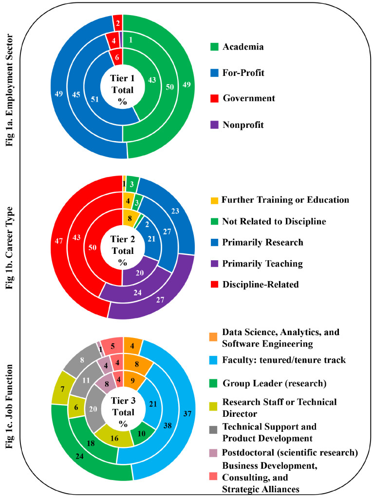
Figure 1. STEM Doctoral Alumni Career Outcomes by Tier

For Tier 3 we find that seven primary job functions describe the work of 87.3% of Wayne State’s STEM PhD alumni: faculty (tenured/tenure track) (31.9%), research group leader (16.9%), technical support/product development (13.3%), research staff or technical director (9.7%), and data science, analytics, and software engineering (7.3%), post-doctoral research (4.2%) business development, consulting and strategic alliances (4%) (Figure 1c). The remaining 12.7% of STEM alumni are engaged in other job functions which have fewer than 4% alumni in each.

STEM Demographic Characteristics and Employment Sector (Tier 1)

We analyzed the Tier 1-Employment Sector data as three windows of 5-years each to see if there were significant career shifts over time, or significant differences in career outcome by gender, race or U.S. citizenship status. We find that the pattern of employment sector for STEM alumni did not significantly change over time, Χ² (6, N = 496) = 7.35, p = .29. However, there was a significant difference between men and women in terms of their sector of employment, Χ² (3, N = 496) = 8.97, p = .03, with women more likely to hold academic jobs and men more likely to be employed in the for-profit sector, p < .05 (Figure 2).

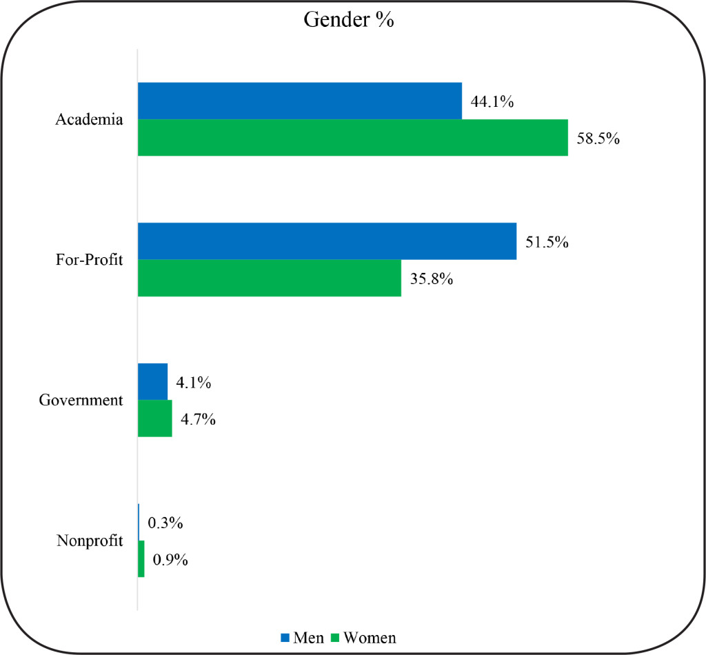
Figure 2. Gender and Employment Sector of STEM Doctoral Alumni

There was also a significant effect of race on employment sector Χ² (6, N = 496) = 19.91, p = .003. A higher proportion of Asians entered the for-profit sector as compared to Whites (p < .05). (Figure 3). There were no significant differences between U.S. citizen and non-U.S. citizen alumni in the STEM fields, Χ² (3, N = 496) = 1.86, p = .60.

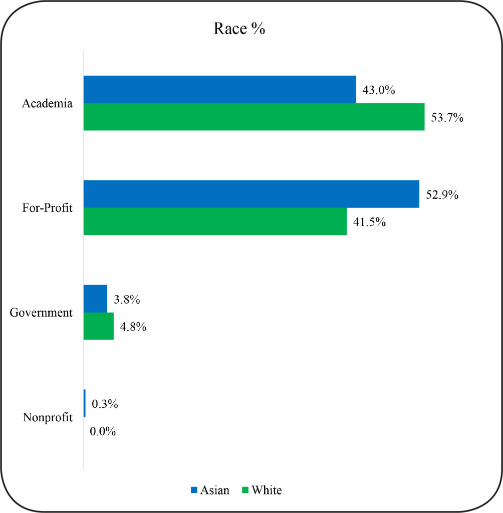
Figure 3.Race and Employment Sector of STEM Doctoral Alumni

STEM Demographic Characteristics and Career Type
(Tier 2)

We further analyzed the Tier 2- Career Type data as three windows of 5-years each for total alumni as well as by gender, race, and U.S. citizenship status. As with Tier 1, we find that for STEM alumni, the distribution of career types did not significantly change over time, Χ² (, N = 496) = 12.15, p = .15. However, men and women differed in their career types, Χ² (4, N = 496) = 11.64, p = .02. Significantly more women were in primarily teaching careers (p < .05), and more men in science-related careers (p < .05). (Figure 4). Racial group distributions were similar across Career Types, Χ² (8, N = 496) = 6.96, p = .54. Career type was not associated with citizenship status, Χ² (4, N = 496) = 2.3, p = .68.

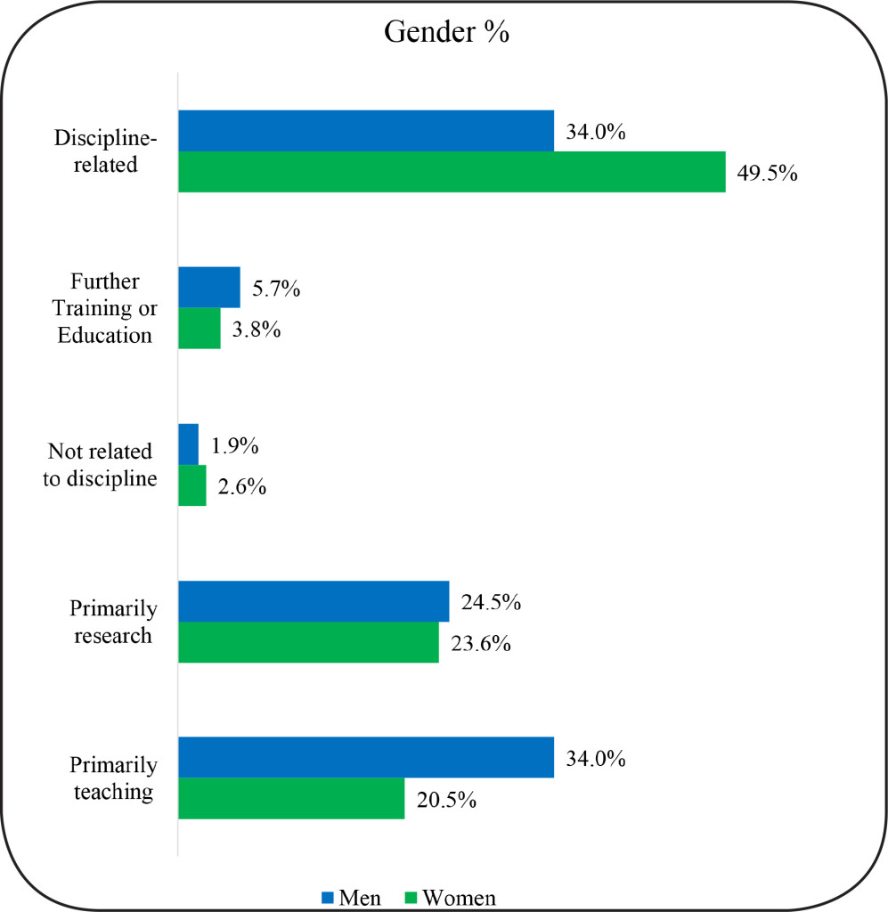
Figure 4. Gender and Career Type of STEM Doctoral Alumni

STEM Demographics and Job Function (Tier 3)

We also analyzed the Tier 3- Job Function data in the same manner as described for employment sector and career type. For this Tier, we found significant changes in the proportions of alumni in different job functions across the different five-year time windows, Χ² (8, N = 392) = 37.38, p = .0001. Specifically, the proportion of alumni in faculty jobs increased significantly from window 1 (0–5 years) to 2 (5–10 years) (p < .05). We believe this shift may reflect a transition where alumni shift from postdoctoral positions or other additional training to faculty positions. Similarly, the number of alumni in group leader (research) jobs increased significantly from window 1 (0–5 years) to 3 (10–15 years) (p < .05), whereas the proportion of STEM alumni in data science/technical support and product development jobs declined from window block 1 to 3 (p < .05). There was also a significant decrease in alumni in research staff or technical director jobs from Window 1 to 2 (p < .05) (Figure 1c). Again, these shifts can be viewed as part of the expected course of career advancement of Ph.D. holders.

A significant difference was also found between women and men with regard to job function (Figure 5). The significant Chi-square for gender, Χ² (4, N = 392) = 17.58, p = .001 was accounted for by the fact that women were more likely to hold tenured/tenure track faculty jobs and men were more highly represented in group leader jobs (p < .05). (Figure 5). There were no significant racial group differences, Χ² (8, N = 392) = 8.47, p = .39, or citizenship group differences Χ² (4, N = 392) = 6.29, p = .18 in job functions.

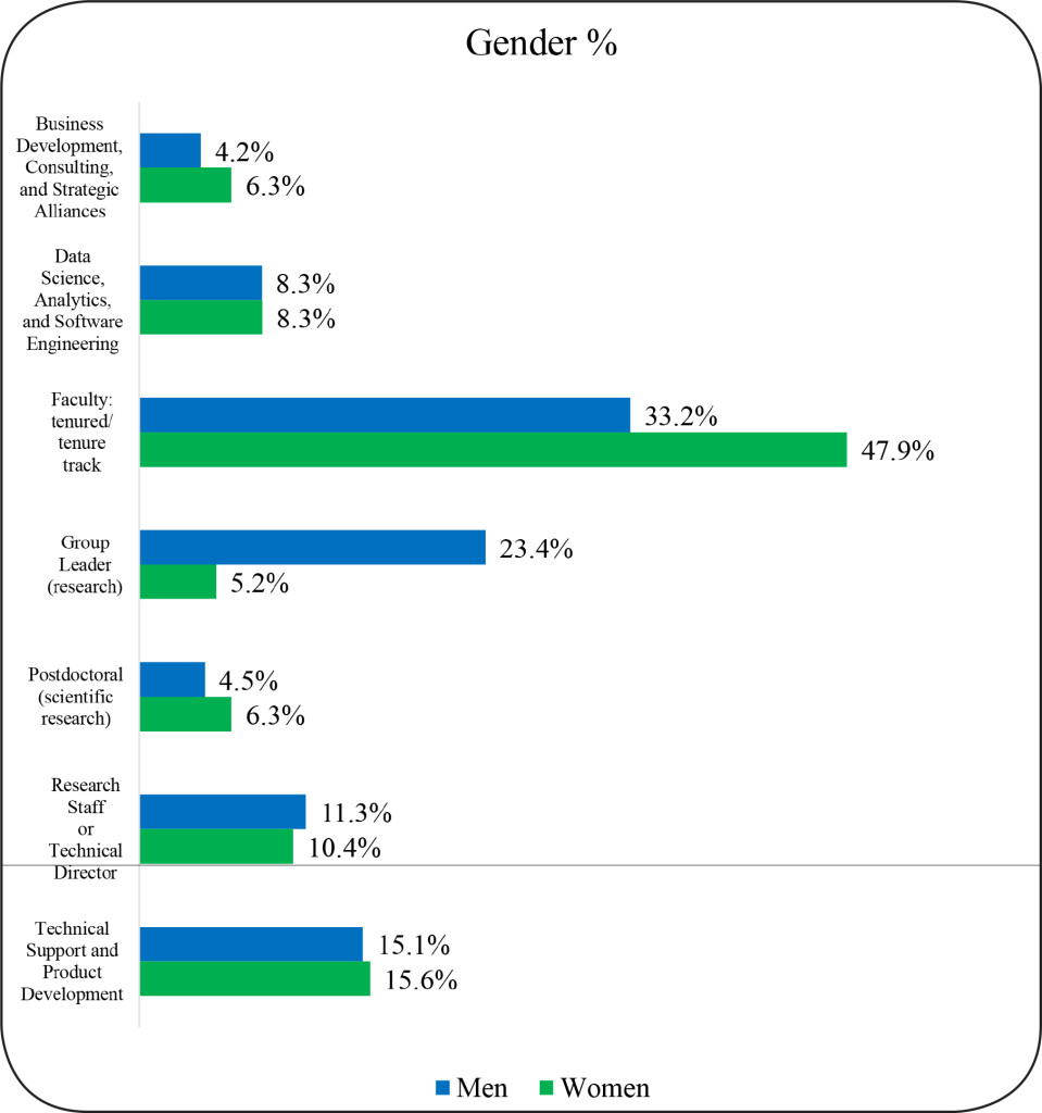
Figure 5. Job Function of STEM Doctoral Alumni by Gender

STEM Academic performance indicators and employment sector

We also examined the association of academic characteristics with the two largest STEM employment sectors: “Academia” and “For-profit.” Participation in other sectors is too small to allow for meaningful comparisons.

There are no statistically significant differences in most of the academic performance indicators examined between alumni who end up in careers in academia as versus the for-profit sector. There is an equivalent spread of GRE-Quantitative scores, GRE-Verbal scores and cumulative GPA of alumni between these sectors (Figure 6). However, STEM alumni who took longer to complete their degrees were more likely to enter the for-profit sector, B = .165, SE = .049, Wald (df = 1) = 11.37, p = .001. A follow-up t-test showed that alumni in the academic sector completed their degrees, on average, in 5.68 years (SD = 1.68) whereas alumni in the for-profit sector completed their degrees, on average, in 6.33 years (SD = 2.30), t (471) = 14.88, p = .001.

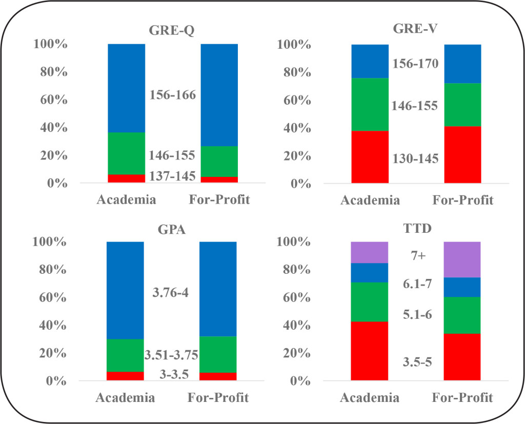
Figure 6. STEM Doctoral Alumni Academic Performance Indicators and Employment Sector

15-year career outcomes of WSU’s SBSE doctoral alumni

SBSE alumni outcomes show not all employment sectors, career types, and job functions are equally represented. SBSE alumni data in Tiers 1, 2 and 3 across the three time windows (0–5 years; 6–10 years; and 11–15 years) is summarized (Figure 7).

In Tier 1, we found the majority of SBSE alumni are employed in academia (64.6%) and the for-profit sector (27.5%). The remaining 8.1% work in government (5.0%) and nonprofit (2.9%) sectors (Figure 7a). This is different from STEM alumni, for whom similar percentages worked in academia and the for-profit sector. Still, over a third of SBSE alumni move on to careers outside of academia. Tier-2 (Career Type) shows that alumni engage in careers that are discipline-related (39.2%) and primarily teaching (38.3%). Approximately 18.9% engage in careers that are primarily research and a small percentage in careers not related to their Ph.D. discipline (3.6%) (Figure 7b).

For Tier-3 (Job Functions), we find that seven primary job functions describe the work of 86.1% of WSU’s SBSE’s alumni: faculty tenure/tenure track (35.9%), healthcare provider (15.1%),  administration (11.2%), business development, consulting, and strategic alliances (6.7%), research staff or technical director (6.2%), full-time teaching staff/instructor (6.0%), part-time teaching staff/adjunct (5.0%) (Figure 7c). The remaining 13.9% of SBSE alumni are engaged in job functions that have fewer than 4% alumni in each.

Demographics Characteristics and Employment Sector (Tier 1)

Approximately 92.1% of SBSE alumni are engaged in either academia or for-profit sectors. For the SBSE alumni, unlike STEM graduates, the pattern of employment sector did not significantly change over time, Χ² (6, N = 418) = 3.96, p = .68. The percentage of SBSE alumni in academic and for-profit careers appears relatively stable across the three time windows. Note that as discussed earlier, the trajectory of each alumnus over a 15-year time period is not reported. Rather, we show aggregate alumni employment data in each time window grouped by years following graduation. For example, a student who graduated in 2006 would be represented in the 6–10 year block only.

In addition, for SBSE alumni we do not see the same gender and race differences we find for STEM alumni. In SBSE fields, men and women did not significantly differ in employment sector, Χ² (3, N = 418) = 2.11 p = .55. Racial group distributions were similar across employment sector, Χ² (6, N = 412) = 10.85, p = .09. Also, as with STEM alumni, employment sector was not associated with citizenship status, Χ² (3, N = 418) = 5.59, p = .13.

Demographics Characteristics and Career Type (Tier 2)

For SBSE alumni, the majority are split between careers that primarily involve teaching and other discipline-related career types. As in the case of SBSE Tier 1 employment sector, the distribution of career types did not significantly change over time, Χ² (6, N = 418) = 5.30, p = .51. There were no significant gender differences in career types, Χ² (3, N = 418) = 5.82, p = .12. Racial group distributions were similar across career types, Χ² (6, N = 412) = 8.27, p = .22. Nor was career type associated with citizenship status, Χ² (3, N = 418) = 4.62, p = .20. To summarize, career types – whether primarily teaching, primarily research, discipline-related or not related to discipline of study– did not vary for SBSE doctoral alumni with respect to gender, race, or citizenship status.

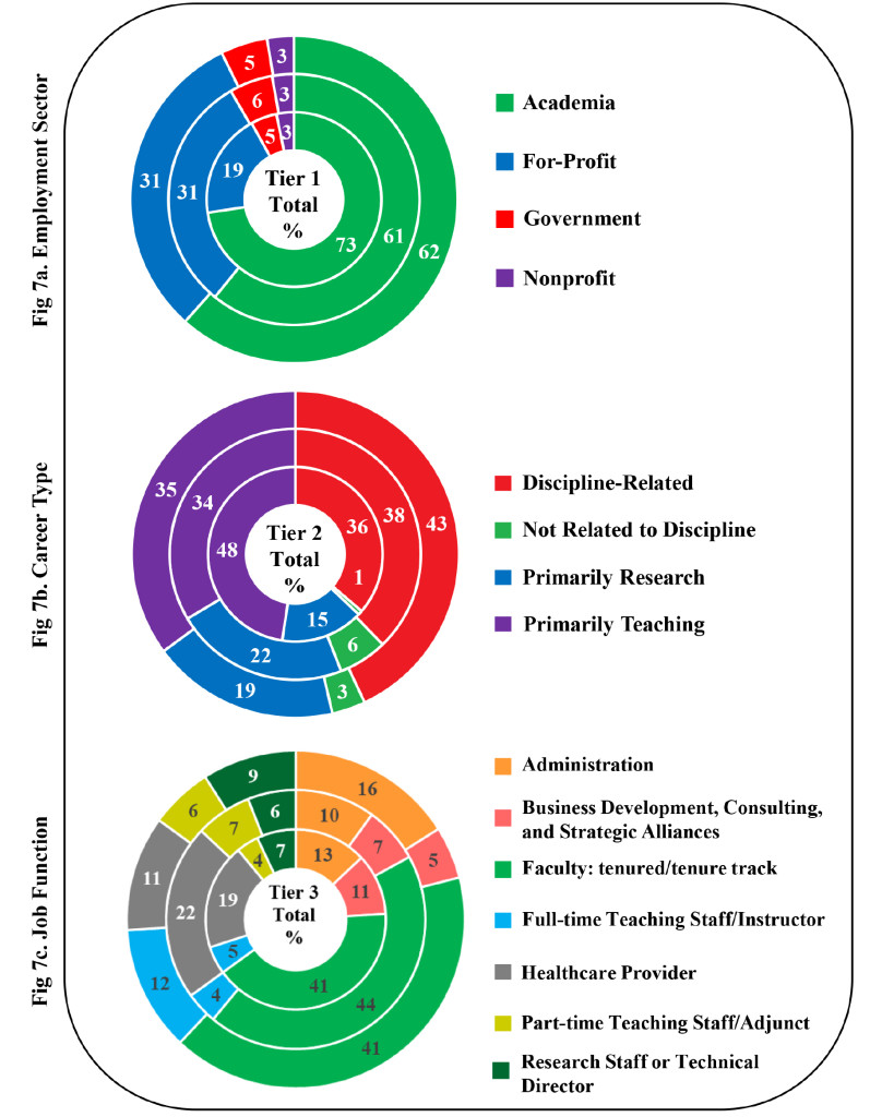
Figure 7. SBSE Doctoral Alumni Career Outcomes by Tier

Demographics Characteristics and Job Function (Tier 3)

For job function, as with employment and career type, we find no statistically significant changes in the proportions of alumni in different job functions over our three time windows, Χ² (12, N = 360) = 13.08 p = .36. However, there was a significant Chi-square for gender, Χ² (6, N = 360) = 13.65, p = .03 in the job function category of healthcare provider. Specifically, our data show that women are more likely to work as health care providers than men. (Figure 8).

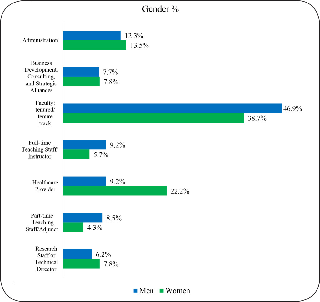
Figure 8. SBSE Doctoral Alumni Job Function by Gender

There were also some significant racial group differences in job functions, Χ² (12, N = 354) = 31.1, p = .002 (Figure 9). White alumni were more likely than Asian alumni to work as healthcare providers. White alumni were also more likely to hold full-time teaching staff/instructor position than Black alumni. Note that Figure 9 depicts the overall percentage of alumni within the seven top job functions with respect to racial demographics. Although White alumni held 50% of the positions reported for full-time teaching staff/instructor job functions, only 4% of White alumni were represented in this category overall.  However, 17% of black alumni are represented in these job functions. There were no significant citizenship group differences in job functions, Χ² (6, N = 360) = 8.35, p =.21

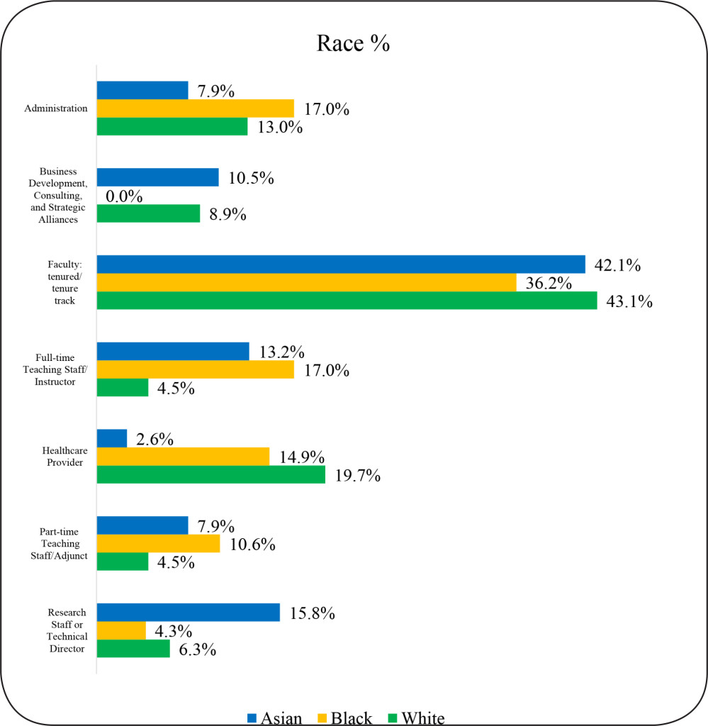
Figure 9. SBSE Doctoral Alumni Job Function by Race

SBSE Academic Performance Indicators and Employment Sector

We examined the association of academic characteristics with career outcomes in only the two largest employment sectors of “Academia” and “For-profit”, since participation in other sectors is too small to allow for meaningful comparisons.

Interestingly, we found no statistically significant differences in any of the academic characteristics examined between alumni in academia and for-profit sectors. An equivalent spread of GRE-Quantitative scores, GRE-Verbal scores, cumulative GPA, and Time-to-Degree completion of alumni between these sectors is shown (Figure 10). Thus, we can conclude that these traditional performance metrics tell us little about what career path our alumni are likely to take.

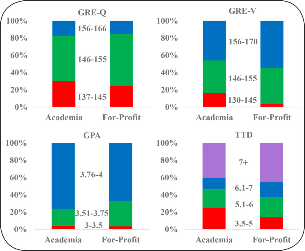
Figure 10. SBSE Doctoral Alumni Academic Performance Indicators and Employment Sector

Discussion

In this paper, we have investigated the 15-year career trajectories of STEM and SBSE doctoral alumni of Wayne State University, a comprehensive research university in Detroit, Michigan. The findings of our study have implications for how higher education institutions approach training and advising for Ph.D. students.

First, our findings confirm exiting studies that show that today’s doctoral students pursue diverse career trajectories – not just tenured positions in the academy. This indicates that we should be advising doctoral students in STEM and SBSE fields about diverse career pathways they might pursue after the Ph.D. Universities should take steps to prepare doctoral students for success not just in academia, but in other areas, particularly the for-profit sector.

As suspected, a common theme throughout the data for STEM alumni was the different career paths for men and women. Our findings show that for employment sector and career type, women were more likely to work in academia in primarily teaching roles, while men were more likely to work in the for-profit sector and in science-related positions. This is further reflected in the job function outcomes in which women worked as faculty whereas men pursued positions such as group leader.

The finding that women in STEM fields were more likely to pursue careers in academia is interesting and encouraging.   Research has consistently shown that women and minorities are underrepresented in STEM [26]. This trend is reflected in our 15-year Ph.D. alumni data: in STEM fields, the sample included 76% men compared to 24% women (Table 2). The need to increase diversity in STEM fields is an issue that has been identified at both the national level and at Wayne State [27]. Recognizing these disparities, WSU has actively sought to increase the representation of women and minorities in STEM fields through programs such as the NIH BUILD (Building Infrastructure Leading to Diversity) program, Wayne Med Direct and the Postdoctoral to Faculty Transition (PFT) fellowship. WSU provides support and training to current students and early career scholars to produce a pipeline of underrepresented students for doctoral training and faculty positions in a range of disciplines [28].

As expected, the data does suggest that a majority of SBSE alumni follow more traditional pathways with alumni securing academic positions at greater levels than those in STEM disciplines.  Overwhelmingly, SBSE alumni are working in academia, in both tenured/ tenure-track positions and non-tenured roles (adjuncts or full-time instructors).  We found that White alumni are more likely to hold non-tenure track positions than Asians and Black alumni. The percentage of SBSE alumni in non-tenured roles can be viewed from a number of different perspectives. On one hand, part-time and adjunct teaching offer less job security and upward mobility than tenured/tenure-track positions. However, some PhDs, such as those embarking on a second career or preferring a part-time position, may view non-tenured positions as offering more flexibility.

In conclusion, both STEM and SBSE students will clearly benefit from early advising about diverse career pathways.  There are some statistically significant gender differences and a few differences by race, but, in general, our research demonstrates that Ph.D. students of diverse backgrounds seek a wide array of career pathways.  Citizens and non-citizens are equally likely to pursue a variety of career tracks and job functions.

Furthermore, any preconceived notions that graduate schools, graduate program or faculty advisors might hold about who might and might not succeed in the “traditional” tenure/tenure-track academic career based on academic performance metrics should be discarded. Students with higher and lower scores on traditional academic metrics used to evaluate applicants and evaluate student progress to degree show practically no difference in terms of the likelihood that alumni will pursue different types of careers.

For graduate schools, data on the career trajectories of doctorate holders should shape training and advising. For doctoral students and Ph.D. holders, transparency about diverse career pathways can help them to envision and explore career paths that best fit their interests and needs. We hope that attention to these matters will alleviate some of the stress inherent in the pursuit of a Ph.D. and contribute to higher rates of career satisfaction and well-being for doctoral alumni over the course of their careers.

Contributors: N/A

Acknowledgements: The authors wish to thank Drs. Mark Byrd, Christine Chow, Andrew Feig and Song Yan for their assistance in data collection; and Prassanna Viswanathan for data validation and visualization.

Units of Measurement: N/A

Abbreviations & Symbols: N/A

Competing interests: The authors declare that they have no competing interests.

Funding information: This work was supported by the National Institutes of Health; Grant number: DP7 0D01842; URL: nih.gov; and Wayne State University to AM. The funders had no role in study design, data collection and analysis, decision to publish, or preparation of the manuscript.

References

1. Evans TM, Bira L, Gastelum JB, Weiss LT, Vanderford NL, et al. (2018) Evidence for a mental health crisis in graduate education. Nat Biotechnol 36: 282–284. [crossref]
2. National Science Board Science and Engineering Indicators 2018: Table 3-16 Employed SEH doctorate recipients holding tenured and tenure-track appointments at academic institutions, by field of and years since degree: Selected years, 1993–2015.
3. National Science Board (2018) SEH doctorates in the workforce: 1993–2013.
4. Tilghman S, Rockey S, Degen S, Forese L, et al. (2012) Biomedical research workforce working group report.
5. Alberts B, Kirschner MW, Tilghman S, Varmus H (2014) Rescuing US biomedical research from its systemic flaws. Proc Natl Acad Sci U S A 111: 5773–5777. [crossref]
6. Morrison E, Rudd E, Merad M (2011) Early careers of recent US Social Science PhDs. Learning and Teaching 4: 6–29.
7. Cyranoski D, Gilbert N, Ledford H, Nayar A, Yahia M (2011) Education: The PhD factory. Nature 472: 276–279. [crossref]
8. Roach M, Sauermann H2,3 (2017) The declining interest in an academic career. PLoS One 12: e0184130. [crossref]
9. Sauermann H, Roach M (2012) Science PhD career preferences: levels, changes, and advisor encouragement. PLoS One 7: e36307. [crossref]
10. Fuhrmann CN, Halme DG, O’Sullivan PS, Lindstaedt B (2011) Improving Graduate Education to Support a Branching Career Pipeline: Recommendations Based on a Survey of Doctoral Students in the Basic Biomedical Sciences. CBE Life Sciences Education 10: 239–249.
11. Gibbs KD, Griffin KA (2013) What do I want to be with my PhD? The roles of personal values and structural dynamics in shaping the career interests of recent biomedical science PhD graduates. CBE Life Sciences Education 12: 711–723.
12. Council of Graduate Schools, Educational Testing Service. Pathways Through Graduate School and Into Careers.
13. Denecke D, Kent J, McCarthy MT (2017) Articulating learning outcomes in doctoral education.
14. Mathur A, Cano A, Kohl M, Muthunayake NS, et al. (2018) Visualization of gender, race, citizenship and academic performance in association with career outcomes of 15-year biomedical doctoral alumni at a public research university. PLoS One 13: e0197473.
15. Blank R, Daniels RJ, Gilliland G, Gutmann A, Hawgood S, et al. (2017) A new data effort to inform career choices in biomedicine. Science 358: 1388–1389. [crossref]
16. Xu H, Gilliam RST, Peddada SD, Buchold GM, et al. (2018) Visualizing detailed postdoctoral employment trends using a new career outcome taxonomy. Nat Biotechnol 36: 197–202.
17. Ortega ST, Kent JD. What is a PhD? Reverse-Engineering Our Degree Programs in the Age of Evidence-Based Change. Change: The Magazine of Higher Learning 50: 30–36.
18. Feig AL, Robinson L, Yan S, Byrd M, et al. (2016) Using Longitudinal Data on Career Outcomes to Promote Improvements and Diversity in Graduate Education. Change: The Magazine of Higher Learning 48: 42–49.
19. Silva EA, Des Jarlais C, Lindstaedt B, Rotman E, et al. (2016) Tracking Career Outcomes for Postdoctoral Scholars: A Call to Action. PLOS Biology 14: e1002458.
20. The Stanford University PhD Alumni Employment Project (2018) Stanford University.
21. Vanderbilt University School of Medicine. IGP and QCB Admissions and Outcomes Data. University of North Carolina. Alumni Career Outcomes.
22. Alumni Career Outcomes (2017) University of North Carolina.
23. Mathur A, Brandt P, Chalkley R, Daniel L, et al. (2018) Evolution of a Functional Taxonomy of Career Pathways for Biomedical Trainees. Journal of Clinical and Translational Science 2: 63–65.
24. McCarthy MT (2017) Promising practices in humanities PhD professional development: Lessons learned from the 2016–2017 Next Generation Humanities PhD Consortium.
25. Mathur A, Chow CS, Feig AL, Kenaga H, et al. (2018) Exposure to multiple career pathways by biomedical doctoral students at a public research university. PLOS ONE 13: e0199720.
26. Leshner A, Scherer L editors (2018) Graduate STEM Education for the 21st Century. Washington DC: The National Academies Press
27. National Science Board (2018) Science and Engineering Indicators.
28. Wayne State University (2018) Scientific Training, Workforce Development and Diversity – Key Initiatives.

Appendix S1: Three Tier Taxonomy

Tier 1: Employment Sectors	Tier 2: Career Types	Tier 3: Job Functions
Academia	Primarily Research	Administration
Government	Primarily Teaching	Business Development, Consulting, and Strategic Alliances
For-Profit	Science-related	Clinical Research Management
Nonprofit	Not-related to science	Clinical Services
Other	Further training or education	Data Science, Analytics, and Software Engineering
		Entrepreneurship
		Faculty: non-tenure track
		Faculty: tenured/tenure track
		Faculty: track unclear or not applicable
		Full-time Teaching Staff/Instructor
		Group Leader (research)
		Healthcare Provider
		Intellectual Property and Law
		Part-time Teaching Staff/Adjunct
		Postdoctoral Research
		Regulatory Affairs
		Research Staff or Technical Director
		Sales and Marketing
		Science Education and Outreach
		Science Policy and Government Affairs
		Science Writing and Communication
		Technical Support and Product Development
		Completing further education or training
		Other
		Deceased/retired

Appendix S2

References

1. Lee KW, Blankenship KD, McCurry ZM, et al. (2009) Performance characteristics of a monoclonal antibody cocktail-based ELISA for detection of allergen-specific IgE in dogs and comparison with a high affinity IgE receptor-based ELISA. Vet Dermatol 20: 157–64. [crossref]
2. Lee KW, Blankenship KD, McCurry ZM, et al. 2012, Reproducibility of a Monoclonal Antibody Cocktail Based ELISA for Detection of Allergen Specific IgE in Dogs: Proficiency Monitoring of macELISA in Six US and European Laboratories. Vet. Immunol Immunopathol 148: 267–275.
3. Lee KW, Blankenship K, McKinney B, Kern G, Buch J, et al. (2015) Proficiency monitoring of monoclonal antibody cocktail–based enzyme-linked immunosorbent assay for detection of allergen-specific immunoglobulin E in dogs. Journal of Veterinary Diagnostic Investigation 27: 461–469.
4. Lee K, Blankenship K, McKinney B, Kern G, Roth E, et al. (2017) Continued Proficiency Monitoring Of Monoclonal Antibody Cocktail-Based Enzyme-Linked Immunosorbent Assay for Detection of Allergen Specific Immunoglobulin E in Dogs – 2016. Integr J Vet Biosci 1: 1–10.
5. DeBoer DJ, Hillier A (2001) The ACVD task force on canine atopic dermatitis (XVI): laboratory evaluation of dogs with atopic dermatitis with serum-based “allergy” tests. Vet Immunol Immunopathol 81: 277–87.
6. Gorman NT, Halliwell REW (1989) Atopic Diseases. In: Halliwell REW, Gorman NT (eds.). Veterinary Clinical Immunology. WB Saunders, Philadelphia, USA Pg No: 232–52.
7. Griffin CE, DeBoer DJ (2001) The ACVD task force on canine atopic
dermatitis (XIV): clinical manifestation of canine atopic dermatitis. Vet Immunol Immunopathology 81: 255–69.
8. Griffin CE, Hillier A. (2001) The ACVD task force on canine atopic dermatitis (XXIV): allergen-specific immunotherapy. Vet Immunol Immunopathol 81: 363–83.
9. Tijssen P (1993) Processing of data and reporting of results of enzyme immunoassays. In: Burdon, RH, van Knippenberg PH (eds.). Practice and Theory of Enzyme Immunoassays. Elsevier, Amsterdam, Netherlands Pg No: 385–421.
The Challenge of Measuring Caries Disease in Populations
DOI: 10.31038/JDMR.2018115
Abstract
Introduction: There are so many methods for measuring caries disease in populations that it is a great challenge for researchers and epidemiologists to choose which one is most appropriate for their research or surveys.
Objective: to make a discussion about the difficulties in measuring caries disease in populations using scientific articles that contributed to the reflection on the subject.
Conclusion: Due to the importance of the issue a careful analysis of the literature is necessary to decide which method should be used to measure caries disease in the populations.
Keywords
DMF index, caries dental; health surveys.
Caries is a chronic disease worldwide and, according to the World Health Organization (WHO), affects 60–90% of school-age children and 100% of adults in various regions [1], with considerable variations between countries. In 2010, untreated caries lesions on permanent teeth were the most prevalent condition worldwide, affecting 2.4 billion people, with potential impact on the global economy [2]. Despite the importance of this disease, there is no consensus as to the most appropriate method for the detection of caries in populations, so there are numerous methods described in the literature [3–10]. Due to many options that currently exist researchers and epidemiologists need to be aware of several aspects when choosing a method to detect caries in populations. Before choosing a method, it is recommended that the researcher analyze several questions to determine which method is most appropriate to the objectives of his research or his epidemiological survey. These questions will be addressed here, while a comparison will be made between three methods that stood out in the literature, being validated and used internationally [11–13]: The Caries Assessment Spectrum and Treatment (CAST) [14], the International Caries Detection and Assessment System (ICDAS) [8] and the DMF (Decayed, Missing and Filled)[15].
The first question is:- What diagnostic threshold will be used to detect caries lesions? This threshold can vary from enamel lesions visualized after we dried the enamel until extensive dentin lesions have reached the pulp and caused an odontogenic infection. DMF has traditionally measured caries from dentin lesions (D3), leaving lesions in enamel (D1) sub registered. The CAST measures from non-cavitary enamel lesions that do not need to be dried to be detected, not using compressed air. The ICDAS measures from the first clinical sign of caries that are non-cavitated enamel lesions that need to be dried for 5 seconds to be seen [16]. The CAST and the ICDAS decrease the underestimation of caries when diagnosing these diseases from enamel lesions.
The second question is:- Which unit of measurement we will use? Can the individual unit be chosen when we detect how many individuals are sick in a community, for example, in 100 individuals who have lesions of caries? When we use teeth unit in a group of 100 people how many of its 3200 teeth have been affected? We can use the surface unit and, if so, how many of the 1,4800 surfaces examined have been affected by caries? In each one, caries can reach different levels of severity, from a reversible enamel lesion to total surface/tooth destruction.
A third important question relates to the choice of unit of measure we will include in calculating the prevalence of caries disease. The number of people with caries lesions? Alternatively, the number of teeth or surfaces affected by caries? [15]
With DMF and ICDAS the tooth or surface unit has been used. However, this makes it difficult to communicate with other areas of health and with planners and decision-makers, since generally the prevalence is calculated using the individual unit of measure. The prevalence of a disease is the proportion of a population that has a disease at a specific level at a point in time [17]. In epidemiology, a patient has one or more diseases, while the rest of the population is healthy. The sick individuals correspond to the number of cases [18].
In Dentistry, however, this principle is generally not followed, and therefore there is a specific approach to the tooth. It means that will be checked whether each tooth is diseased or not, by adding the tooth that has the disease at the time of examination (caries lesions) with the teeth that have been affected by it in the past and have been extracted or restored. However, it may be misleading to consider the teeth restored and absent as experience of caries because the teeth may have been restored or extracted for other reasons [18].
The CAST uses the individual unit to calculate the prevalence of caries without considering the extracted or restored teeth [19], which is more in agreement with the classical concept of prevalence because it detects the disease present at the moment of the examination per individual, thus identifying the individuals who need dental treatment at the time of the examination. When individuals receive this treatment, they are excluded from the disease prevalence this allows communicating more quickly to health planners the results of interventions in a given community.
A fourth and final question is: – We will evaluate the activity of the lesion? That is, once the lesion is detected, we must consider as active or inactive through its appearance?
The usefulness of measuring caries activity is questionable because when some authors [20, 21] used this indicator no significant change was identified. These authors argue that treating all non-cavitated lesions, as if they were all with active caries, instead of evaluating the caries activity, would be better cost-effective in the long term. CAST and DMF do not include caries activity. However, ICDAS has been proposed to be used in conjunction with methods that evaluate this activity (Nyvad System [6], Lesion Activity Assessment – LAA [22], and LA from the International Caries Classification and Management System – ICCMS [23] ).
According to Frencken [24], for an epidemiological index, it is not advantageous to include assessment of caries activity, as this would only make the index more complicated. However, for Nyvad [6], the evaluation of the lesion activity is essential for the determination of the need for treatment, since the active lesions require intervention (operative or non-operative), while inactive lesions require only the daily use of fluoride toothpaste.
The registry of non-cavitated enamel lesions aims to provide a more comprehensive epidemiological picture of the distribution of the disease in the population; however, to include these lesions, it is necessary that the teeth be dry, requiring more calibration time for examiners and a more detailed examination [1]. The choice of a particular method should take into account the purpose of the study, the human resources, and the materials available. Epidemiological surveys conducted in underdeveloped or developing countries have scarce resources, and therefore epidemiologists have chosen DMF because it is a quick and inexpensive index.
Limits and deficiencies of DMF have been reported in the literature, some authors point out the need to use new methods that measure caries disease in populations in a way that is more in agreement with new concepts of cariology and epidemiology, including non-cavitated enamel lesions and using an individual unit of measure [18, 25]. Given the importance of measuring caries in populations, studies are needed to assist researchers in the choices among the various methods. Castro et al. [26] compared to CAST, ICDAS, and DMF. After this study the authors arrived at the following conclusions:
Advantages and disadvantages of DMF
The DMF uses the unit of measure tooth or surface and offers as advantages: ease of use; speed of application; simplicity of analysis; does not require the use of compressed air; is recommended by WHO and MS; is comparable with international data collected since the 1940s. As for disadvantages of DMF, the authors cite: the use of the DMF mean that considers very different clinical conditions, implying the need to decompose the index in the lost and restored caries components, to verify how much each one is present in the population; traditionally, does not include lesions on enamel. The DMF includes decayed, restored and lost teeth, so it is an irreversible index; the prevalence calculated through it will never decrease in the same group over time; therefore, measures the prevalence of the disease cumulatively. That is, individuals who are no longer with the disease at the time of the examination can be included in the prevalence of the disease; also, some teeth may have been extracted or restored for reasons other than caries, overestimating the presence of the disease.
Advantages and disadvantages of ICDAS
As advantages of the ICDAS, it includes the caries lesions from its most initial clinical stage, when  it is only possible to visualize the lesion through surface drying. This system is used in association with other methods that evaluate caries activity (Nyvad System, LAA, LA) [6, 22, 23].
It is a validated method used in several countries; its data are capable of being transformed into an average DMF; is an appropriate system for clinical use and for monitoring the evolution of individual caries lesions. The disadvantages of the ICDAS are based on the fact that for this method to record enamel lesions, it is necessary to use compressed air to dry each surface for 5 seconds, but in many places, it is not possible to use this equipment. By using many codes and two digits, the analysis becomes complex and overly detailed to be used at the collective level [27].
Advantages and disadvantages of CAST
The CAST can use the individual, tooth or surface unit measure, has the benefits of detecting enamel lesions that can be visualized without the use of a compressed air syringe, to lesions that caused fistula and abscess. Don´t need compressed air; it is a simple, fast method; was validated and used internationally; its criteria are arranged hierarchically, easy to apply and analyze; data can be transformed into an average DMF [14, 26].
The cited disadvantages of CAST were: it was not tested for clinic use [28]; does not measure enamel lesions that can only be seen after tooth drying. Not including this type of lesion is part of the characteristics that make this method more suitable for use in epidemiological surveys. The lack of knowledge about new methods to measure caries in the populations influences the decision on which index to use, as shown in  the study by CASTRO et al. [29] most of the people interviewed said they were dissatisfied with DMF, but they did not use new methods because they could not compare the data later. However, both the CAST and the ICDAS had their data converted to the DMF mean in several studies, with results very similar to those found with the last index [26]. Therefore, the perception that there would be a loss of comparability of results, using other methods, is questionable, since data obtained through the ICDAS and CAST can be converted and compared to data previously registered with the DMF [26].
Conclusions
Due to the importance of the subject and the number of methods proposed, a careful analysis of the literature is necessary to decide which method should be used to measure caries disease in the populations because all of them have advantages and disadvantages. More studies should be done on the subject until a consensus is established.
Authors’ contributions
ALSC drafted the manuscript; ALSC, CMCM, and MIPV reviewed the original draft as well as read and approved the final manuscript.
1. Antunes JLF, Peres MA, Crivello Júnior O (2006) Epidemiology of oral health. In: Fundamentals of Dentistry. Guanabara Koogan pg: 441–442.
2. Kassebaum NJ, Bernabé E, Dahiya M, Bhandari B, Murray CJ, et al. (2015) Global burden of untreated caries: a systematic review and metaregression. J Dent Res 94: 650–658. [crossref]
3. Mount GJ, Hume WR (1997) A revised classification of carious lesions by site and size. Quintessence Int 28: 301–303. [crossref]
4. Fisher J, Glick M, Committee FWDFS (2012) A new model for caries classification and management: the FDI World Dental Federation caries matrix. Elsevier pg: 546–551.
5. de Souza AL, Leal SC, Bronkhorst EM, Frencken JE (2014) Assessing caries status according to the CAST instrument and WHO criterion in epidemiological studies. BMC Oral Health 14: 119. [crossref]
6. Nyvad B (2004) Diagnosis versus detection of caries. Caries Res 38: 192–198. [crossref]
7. Castro ALS, Vianna MIP, Reis SR de A (1999) A new index for measuring dental caries: a reversible index of dental caries-IRCD. Rev Fac Odontol Univ Fed Bahia 19: 35–40.
8. Ismail AI, Sohn W, Tellez M, Amaya A, Sen A, et al. (2007) The International Caries Detection and Assessment System (ICDAS): an integrated system for measuring dental caries. Community Dent Oral Epidemiol 35: 170–178.
9. Sheiham A, Maizels J, Maizels A (1987) New composite indicators of dental health. Community Dent Health 4: 407–414. [crossref]
10. Monse B, Heinrich-Weltzien R, Benzian H, Holmgren C, van Palenstein Helderman W (2010) PUFA–An index of clinical consequences of untreated dental caries. Community Dent Oral Epidemiol 38: 77–82.
11. de Souza AL, Bronkhorst EM, Creugers NH, Leal SC, Frencken JE (2014) The caries assessment spectrum and treatment (CAST) instrument: its reproducibility in clinical studies. Int Dent J 64: 187–194. [crossref]
12. Frencken JE1, de Souza AL, van der Sanden WJ, Bronkhorst EM, Leal SC (2013) The Caries Assessment and Treatment (CAST) instrument. Community Dent Oral Epidemiol 41: 71–77. [crossref]
13. Braun A, Guiraud LMJC, Frankenberger R (2017) Histological validation of ICDAS II and radiological assessment of occlusal carious lesions in permanent teeth. Odontology 105: 46–53.
14. Frencken JE, de Amorim RG, Faber J, Leal SC (2011) The Caries Assessment Spectrum and Treatment (CAST) index: rational and development. Int Dent J 61: 117–123. [crossref]
15. Klein H, Palmer CE (1938) Dental caries in American Indian children. US Govern. Print Off.
16. Frencken JE (2016) Dental Caries and Caries Epidemiology. In: Evidence-Based Caries Prevention. Springer pg: 1–11.
17. Rothman KJ (1998) Precision and validity in epidemiologic studies. Mod Epidemiol.
18. Larmas M, Mäkinen KK (2014) Insufficiency of currently used dental indices in epidemiology. Br J Med Med Res 4: 2058.
19. Ribeiro APD, Maciel IP, de Souza Hilgert AL, Bronkhorst EM, et al. (2018) Caries assessment spectrum treatment: the severity score. Int Dent J 68: 84–90. [crossref]
20. Brown JP, Amaechi BT, Bader JD, Shugars D, Vollmer WM, et al. (2015) The dynamic behavior of the early dental caries lesion in caries-active adults and implications. Community Dent Oral Epidemiol 43: 208–216.
21. Piovesan C, Ardenghi TM, Guedes RS, Ekstrand KR, Braga MM, et al. (2013) Activity assessment has little impact on caries parameters reduction in epidemiological surveys with preschool children. Community Dent Oral Epidemiol 41: 204–211.
22. Ekstrand KR, Martignon S, Ricketts DJN, Qvist V (2007) Detection and activity assessment of primary coronal caries lesions: a methodologic study. Oper Dent 32: 225–235.
23. Pitts NB, Ekstrand KR (2013) International Caries Detection and Assessment System (ICDAS) and its International Caries Classification and Management System (ICCMS)–methods for staging of the caries process and enabling dentists to manage caries. Community Dent Oral Epidemiol 41: 41–52.
24. Frencken JE, de Souza AL, van der Sanden WJ, Bronkhorst EM, Leal SC (2013) The Caries Assessment and Treatment (CAST) instrument. Community Dent Oral Epidemiol 41: e71–77. [crossref]
25. Ismail A1 (2004) Diagnostic levels in dental public health planning. Caries Res 38: 199–203. [crossref]
26. Castro ALS, Vianna MIP, Mendes CMC (2018) Comparison of caries lesion detection methods in epidemiological surveys: CAST, ICDAS and DMF. BMC Oral Health 18: 122.
27. de Amorim RG, Figueiredo MJ, Leal SC, Mulder J, Frencken JE (2012) Caries experience in a child population in a deprived area of Brazil, using ICDAS II. Clin Oral Investig 16: 513–520. [crossref]
28. Leal SC, Ribeiro APD, Frencken JE (2017) Caries Assessment Spectrum and Treatment (CAST): A Novel Epidemiological Instrument. Caries Res 51: 500–506.
29. Castro ALS, Vianna MIP, Mendes CMC (2018) The knowledge and use of population-based methods for caries detection. BMC Oral Health 18: 153. [crossref]
Dental Age Estimation: A Review
DOI: 10.31038/JDMR.2018114
Age is one of the essential factors in establishing the identity of the person. It plays an important role in forensic medicine, clinical dentistry and archaeology. Age estimation is crucial in medico legal cases and importance in forensic medicine, not only for identifying deceased victims but also in connection with crimes and accidents. Age estimation of unknown human bodies is very important in the setting of a crime investigation as well as mass disaster. The age for the individual can be assessed as skeletal, morphological, secondary sex character and dental age.This paper reviews various dental age estimation methods that have been used by the scientist in order to help the identification of remains.
Age Estimation, Identification, Forensic Dentistry
1. Smith T, Brownless L (2011) Age assessment Practices: A Literature Review & Annotated Bibiliography. New York: United Nations Children’s Fund (UNICEF).
2. McKenna CJ, James H, Taylor JA, Townsend GC (2002) Tooth development standards for South Australia. Aust Dent J 47: 223–227. [crossref]
3. Limdiwala PG, Shah JS (2013) Age estimation by using dental radiographs. J Forensic Dent Sci 5: 118–122. [crossref]
4. Briffa K, Dougall NB, Galea J, Mifsud D, Camilleri S (2005) Chronologic and Dental Ages of Maltese Schoolchildren – A pilot Study. Malta Medical Journal 17: 31–35.
5. Gupta P, Kaur H, Shankari G S M, Jawanda MK, Sahi N (2014) Human age estimation from tooth cementum and dentin. J Clin Diagn Res 8: ZC07-10. [crossref]
6. Solheim T, Vonen A (2006) Dental Age Estimation – Quality Assurance and Age Estimation of Asylum Seekers in Norway. Forensic Science International 4747: 56–60.
7. Haavikko K (1970) The formation and the alveolar and clinical eruption of the permanent teeth. An orthopantomographic study. Suom Hammaslaak Toim 66: 103–170. [crossref]
8. Anderson DL, Thompson GW, Popovich F (1976) Age of attainment of mineralization stages of the permanent dentition. J Forensic Sci 21: 191–200. [crossref]
9. GUSTAFSON G (1950) Age determination on teeth. J Am Dent Assoc 41: 45–54. [crossref]
10. Kvaal SI, Kolltveit KM, Thomsen IO, Solheim T (1995) Age estimation of adults from dental radiographs. Forensic Sci Int 74: 175–185. [crossref]
11. Solheim T (1993) A new method for dental age estimation in adults. Forensic Sci Int 59: 137–147. [crossref]
12. Panchbhai AS (2011) Dental Radiographic Indicators, A Key to Age Estimation. DentoMaxillofacial Radiology 40: 199–212.
13. Willems G, Van Olmen A, Spiessens B, Carels C (2001) Dental age estimation in Belgian children: Demirjian’s technique revisited. J Forensic Sci 46: 893–895. [crossref]
14. Wedl JS, Friedrich RE (2005) [Measuring the distance of the wisdom teeth from the occlusal plane as forensic-odontological method for chronological age determination]. Arch Kriminol 215: 77–84. [crossref]
15. Priyadarshini C, Puranik MP, Uma SR (2015) Dental age Estimation Methods: A Review International Journal of Advanced Health Sciences 1(12).
16. Karaarslan B, Karaarslan ES, Ozsevik AO, Ertas E (2010) Age estimation for Dental Patients Using Orthopantomographs. European Journal of Dentistry 4: 389–394.
Violence Against Women: A Case Report of Violence Perpetrated By a Couple on a Single Lady
DOI: 10.31038/AWHC.2018113
Introduction: Violence against women (VAW) is a menace that is increasing all over the world. It is one of the most widespread human rights abuses and a public health problem. Most victims of violence against women know their perpetrators.
Case Presentation: A 28 year old single lady had a quarrel with her female neigbour. The neigbour’s husband held the single lady’s hands behind her and ordered his wife tit beat up the single lady. The female neigbour then bit the left upper eye lid of the single lady resulting in haemorrhage and pain. The injury was sutured.
Conclusion: Men are not the only perpetrators of such violence. Single women are at risk of being victims of violence. To end violence against women, everyone is involved because in some societies such issues are never discussed in public.
Key Words
Violence, Single Lady, Human Bite, Eye
1. Haaga PT, Elechi FA, Okoye AC (2015) Violence against Women and Its Implications for Peace and Security in Nigeria. International Journal of Peace and Conflict Studies 2: 27–40.
2. Alokan FB (2013) Domestic Violence against Women: A Family Menace, 1st Annual International Interdisciplinary Conference, AIIC, Book of Proceedings, 100–107.
3. Ashimolowo OR, Otufale GA (2012) Assessment of domestic violence among women in Ogun State, Nigeria. Greener Journal of Social Sciences 2: 102–114.
4. General Assembly Resolution 48/08 of 28 December 1993.
5. Mbadugha EI (2016) Intimate Partner Violence and Sexual Violence against Women: Any End in Sight. International Journal of Medicine and Biomedical Research 5: 9–18.
Aqueduct-100, A New Device and Method for Controllable Cervical Dilation
DOI: 10.31038/JCRM.2018134
Objective
The aim of this investigation was to evaluate the effectiveness of the Aqueduct-100 for cervical dilation to a predetermined diameter in patients meeting eligibility criteria.
1. Allen RH, Goldberg AB (2016) Cervical dilation before first-trimester surgical abortion (< 14 weeks’ gestation). Contraception. 93(4): 277–291. [Crossref]
2. Arsenijevic S, Vukcevic-Globarevic G, Volarevic V, Macuzic I, Todorovic P, Tanaskovic I, et al. (2012) Continuous controllable balloon dilation: a novel approach for cervix dilation. Trials. 13: 196. [Crossref]
3. Gupta JK, Johnson N (1992) Should we use prostaglandins, tents or progesterone antagonists for cervical ripening before first trimester abortion? Contraception. 46(5): 489–497. [Crossref]
4. Gelber S (2006) Sciscione A: Mechanical methods of cervical ripening and labor induction. Clin Obstet Gynecol. 49: 642–657. [Crossref]
5. Jansen FW, Vredevoogd CB, van Ulzen K, Hermans J, Trimbos JB, Trimbos-Kemper TC. (2006) Complications of hysteroscopy: a prospective, multicenter study. Obstet Gynecol. 49: 642–657. [Crossref]
6. Loffer FD (1995) Contraindications and complications of hysteroscopy. Obstet Gynecol Clin North Am. 22(3): 445–455. [Crossref]
7. Iams J D (2009) Philadelphia, PA: Elsevier Inc; Cervical insufficiency; p. 586.
8. Leppert PC (1995) Anatomy and physiology of cervical ripening. Clin Obstet Gynecol. 38(2): 267–279. [Crossref]
9. Mazza E, Nava A, Bauer M, Winter R, Bajka M, Holzapfel GA (2006) Mechanical properties of the human uterine cervix: an in vivo study. Med Image Anal. 10(2): 125–36. [Crossref]
10. Vico de Miguel FJ, Pantoja-Garrido M, Frias-Sanchez Z, Pantoja-Rosso FJ, Martins E, Weichselbaum A (2017) Experience with a device for controlled cervical dilation. Ginecol Obstet Mex. 85(3): 125–133.
Observational Study to Assess the Safety and Clinical Effectiveness of the Hospital Universitario de Canarias Massive Transfusion Protocol
DOI: 10.31038/JCRM.2018133
Introduction: Massive haemorrhage (MH) is a frequent entity and leads to high mortality rates.The early administration of blood products with high ratios following massive haemorrhage protocols (MHP) has proven to reduce mortality and transfusion of blood components.
Objectives: evaluate the safety and effectiveness of newly implemented MHP for surgical patients with MH and study mortality at 30 day of the haemorrhagic process.
Methods: a new massive haemorrhage protocol was developed and it was based on the early administration of blood products with a 3: 3: 1 ratio (red-blood cells, fresh frozen plasma, platelet). It was a prospective study in which 34 patients with massive haemorrhage were included. The patients were divided in two groups (implementation or non-implementation of the new protocol).
Results: the application of the protocol has not led to a decrease in the mortality rate or in the administration of red blood products and hemostatic drugs. Though there was an increase in the administration of procoagulant factors, but it was not associated with a higher incidence of adverse effects and complications related to mass transfusion.
Key words
massive haemorrhage, transfusion, protocol
1. Hardy JF, de Moerloose P, Samama CM (2005) The coagulopathy of massive transfusion. Vox Sang. 89: 123–7 [Crossref]
2. Ferrara A, MacArthur JD, Wright HK, Modlin IM, McMillen MA (1990) Hypothermia and acidosis worsen coagulopathy in the patient requiring massive transfusion. Am J Surg. 160: 515–8. [Crossref]
3. Fernández-Hinojosa, F. Murillo-Cabezas, A. Puppo-Moreno, S.R. Leal-Noval (2012) “Treatment alternatives in massive hemorrhage”, Med Intensiva 36: 496–503. [Crossref]
4. Borgman MA, Spinella PC, Perkins JG, Grathwohl KW, Repine T, Beekley AC, Sebesta J, Jenkins D, Wade CE, Holcomb JB (2007) “The ratio of blood products transfused affects mortality in patients receiving massive transfusions at a combat support hospital”. J Trauma 63: 805–813. [Crossref]
5. Holcomb JB, Jenkins D, Rhee P, et al. (2007) “Damage control resuscitation: directly addressing the early coagulopathy of trauma”. J Trauma. 62: 307–310. [Crossref]
6. Llau JV, Acosta FJ, Escolar G, Fernández-Mondéjar E, Guasch E, Marco P et al. (2015)  Multidisciplinary consensus document on the management of massive haemorrhage (HEMOMAS document). Med Intensiva 39: 483–504. [Crossref]
7. National Blood Authority (NBA). (2011) “Patient Blood Management Guidelines: Module 1”. Critical Bleeding /Massive Transfusion. Canberra, Australia: NBA;
8. Goodnough LT, Levy JH, Murphy MF (2013) Concepts of blood transfusion in adults. Lancet. 381 (9880): 1845–1854. [Crossref]
9. Holcomb JB, Fox EE, Zhang X, et al. (2013) PROMMTT Study Group. “Cryoprecipitate use in the PROMMTT study”. J Trauma Acute Care Surg 75(Suppl 1): S31- [Crossref]
10. Greer SE, Rhynhart KK, Gupta R, Corwin HL (2010) “New developments in massive transfusion in trauma”. Current opinion in anaesthesiology 23: 2 246–50. [Crossref]
11. O’Keeffe T, Refaai M, Tchorz K, Forestner JE, Sarode R (2008) “A massive transfusion protocol to decrease blood component use and costs”. Arch Surg. 143: 686–90, discussion: 90–1. [Crossref]
12. Snyder CW, Weinberg JA, McGwin G, et al. (2009) “The relationship of blood product ratio to mortality: Survival benefit or survival bias?” J Trauma. 66: 358–362. [Crossref]
13. Magnotti LJ, Zarzaur BL, Fischer PE, Williams RF, Myers AL, Bradburn EH, Fabian TC, Croce MA (2011) “Improved survival after hemostatic resuscitation: does the emperor have no clothes?”. J Trauma 70: 97–102. [Crossref]
14. Sirat Khan, Shubha Allard, Anne Weaver, Colin Barber, Ross Davenport, Karim Brohi (2013) “A major haemorrhage protocol improves the delivery of blood component therapy and reduces waste in trauma massive transfusion”. Mayo vol 44, Issue 5,pages 587–592. [Crossref]
15. Cotton BA, Au BK, Nunez TC, et al. (2009) “Predefined massive transfusion protocols are associated with a reduction in organ failure and postinjury complications”. J Trauma 66: 41–9. [Crossref]
Does flooring-type change the gait characteristics of the older adult? Analysis of balance and temporal-spatial gait parameters and ground reaction force
1. Choi HS (2013) Vitamin d status in Korea. Endocrinol Metab (Seoul) 28: 12–16. [crossref]
2. Abdul-Ghani MA, Williams K, DeFronzo R, Stern M (2006) Risk of progression to type 2 diabetes based on relationship between postload plasma glucose and fasting plasma glucose. Diabetes Care 29: 1613–1618.
3. Pittas AG, Harris SS, Eliades M, Stark P, Dawson-Hughes B (2009) Association between serum osteocalcin and markers of metabolic phenotype. J Clin Endocrinol Metab 94: 827–832.
4. Lee NK, Sowa H, Hinoi E, Ferron M, Ahn JD, et al. (2007) Endocrine regulation of energy metabolism by the skeleton. Cell 130: 456–469. [crossref]
5. Teegarden D, Donkin SS (2009) Vitamin D: emerging new roles in insulin sensitivity. Nutr Res Rev 22: 82–92. [crossref]
6. Pittas AG, Lau J, Hu FB, Dawson-Hughes B (2007) The role of vitamin D and calcium in type 2 diabetes. A systematic review and meta-analysis. J Clin Endocrinol Metab 92: 2017–2029. [crossref]
7. Shea MK, Gundberg CM, Meigs JB, Dallal GE, Saltzman E, et al. (2009) Gamma-carboxylation of osteocalcin and insulin resistance in older men and women. Am J Clin Nutr 90: 1230–1235. [crossref]
8. Ferron M, Hinoi E, Karsenty G, Ducy P (2008) Osteocalcin differentially regulates ß cell and adipocyte gene expression and affects the development of metabolic diseases in wild-type mice. Proc Natl Acad Sci U S A 105: 5266–5270.
9. Viljakainen H, Ivaska KK, Paldánius P, Lipsanen-Nyman M, Saukkonen T, et al. (2014) Suppressed bone turnover in obesity: a link to energy metabolism? A case-control study. J Clin Endocrinol Metab 99: 2155–2163. [crossref]
10. Paldanius P, Ivaska K, Hovi P, Andersson S, Väänänen H, et al. (2012) The effect of oral glucose tolerance test on serum osteocalcin and bone turnover markers in young adults. Calcif Tissue Int 90: 90–95.
11. Paldánius PM, Ivaska KK, Hovi P, Andersson S, Eriksson JG, et al. (2013) Total and carboxylated osteocalcin associate with insulin levels in young adults born with normal or very low birth weight. PLoS One 8: 63036. [crossref]
12. Knapen MH, Schurgers LJ, Shearer MJ, Newman P, Theuwissen E, et al. (2012) Association of vitamin K status with adiponectin and body composition in healthy subjects: uncarboxylated osteocalcin is not associated with fat mass and body weight. Br J Nutr 108: 1017–1024. [crossref]
13. Zhou M, Ma X, Li H, Pan X, Tang J, et al. (2009) Serum osteocalcin concentrations in relation to glucose and lipid metabolism in Chinese individuals. Eur J Endocrinol 161: 723–729.
14. Lee H, Oh J-Y, Sung Y-A, Chung H, Kim H-L, et al. (2015) Genome-wide association study identified new susceptibility loci for polycystic ovary syndrome. Hum Reprod 30: 723–731.
15. Organization WH (2000) The Asia-Pacific perspective: redefining obesity and its treatment. Sydney: Health Communications Australia.
16. Stumvoll M, Mitrakou A, Pimenta W, Jenssen T, Yki-Järvinen H, et al. (2000) Use of the oral glucose tolerance test to assess insulin release and insulin sensitivity. Diabetes care 23: 295–301.
17. Holick MF (2007) Vitamin D deficiency. N Engl J Med 357: 266–281. [crossref]
18. Mattila C, Knekt P, Männistö S, Rissanen H, Laaksonen MA, et al. (2007) Serum 25-hydroxyvitamin D concentration and subsequent risk of type 2 diabetes. Diabetes Care 30: 2569–2570. [crossref]
19. Chiu KC, Chu A, Go VL, Saad MF (2004) Hypovitaminosis D is associated with insulin resistance and beta cell dysfunction. Am J Clin Nutr 79: 820–825. [crossref]
20. Scragg R, Sowers M, Bell C (2004) Serum 25-hydroxyvitamin D, diabetes, and ethnicity in the Third National Health and Nutrition Examination Survey. Diabetes care 27: 2813–2818.
21. Pittas AG, Harris SS, Stark PC, Dawson-Hughes B (2007) The effects of calcium and vitamin D supplementation on blood glucose and markers of inflammation in nondiabetic adults. Diabetes care 30: 980–986.
22. Talaei A, Mohamadi M, Adgi Z (2013) The effect of vitamin D on insulin resistance in patients with type 2 diabetes. Diabetol Metab Syndr 5: 8. [crossref]
23. Maestro B, Campión J, Dávila N, Calle C (2000) Stimulation by 1,25-dihydroxyvitamin D3 of insulin receptor expression and insulin responsiveness for glucose transport in U-937 human promonocytic cells. Endocr J 47: 383–391.
24. Ford ES, Ajani UA, McGuire LC, Liu S (2005) Concentrations of serum vitamin D and the metabolic syndrome among U.S. adults. Diabetes Care 28: 1228–1230. [crossref]
25. Konradsen S, Ag H, Lindberg F, Hexeberg S, Jorde R (2008) Serum 1,25-dihydroxy vitamin D is inversely associated with body mass index. Eur J Nutr 47: 87–91. [crossref]
26. Parikh SJ, Edelman M, Uwaifo GI, Freedman RJ, Semega-Janneh M, et al. (2004) The relationship between obesity and serum 1, 25-dihydroxy vitamin D concentrations in healthy adults. J Clin Endocrinol Metab 89: 1196–1199.
27. Rajakumar K, de las Heras J, Chen TC, Lee S, Holick MF, et al. (2011) Vitamin D status, adiposity, and lipids in black American and Caucasian children. J Clin Endocrinol Metab 96: 1560–1567. [crossref]
28. Mithal A, Wahl DA, Bonjour JP, Burckhardt P, Dawson-Hughes B, et al. (2009) Global vitamin D status and determinants of hypovitaminosis D. Osteoporos Int 20: 1807–1820. [crossref]
29. Choi HS, Oh HJ, Choi H, Choi WH, Kim JG, et al. (2011) Vitamin D insufficiency in Korea-a greater threat to younger generation: the Korea National Health and Nutrition Examination Survey (KNHANES) 2008. J Clin Endocrinol Metab 96: 643–651.
30. Patti A, Gennari L, Merlotti D, Dotta F, Nuti R (2013) Endocrine actions of osteocalcin. Int J Endocrinol 2013: 846480. [crossref]
31. Kindblom JM1, Ohlsson C, Ljunggren O, Karlsson MK, Tivesten A, et al. (2009) Plasma osteocalcin is inversely related to fat mass and plasma glucose in elderly Swedish men. J Bone Miner Res 24: 785–791. [crossref]
32. Im JA, Yu BP, Jeon JY, Kim SH (2008) Relationship between osteocalcin and glucose metabolism in postmenopausal women. Clin Chim Acta 396: 66–69. [crossref]
33. Kim SH, Lee JW, Im JA, Hwang HJ (2010) Serum osteocalcin is related to abdominal obesity in Korean obese and overweight men. Clin Chim Acta 411: 2054–2057. [crossref]
34. Fernández-Real JM, Izquierdo M, Ortega F, Gorostiaga E, Gomez-Ambrosi J, et al. (2009) The relationship of serum osteocalcin concentration to insulin secretion, sensitivity, and disposal with hypocaloric diet and resistance training. J Clin Endocrinol Metab 94: 237–245.
35. Kanazawa I, Yamaguchi T, Yamamoto M, Yamauchi M, Kurioka S, et al. (2009) Serum osteocalcin level is associated with glucose metabolism and atherosclerosis parameters in type 2 diabetes mellitus. J Clin Endocrinol Metab 94: 45–49.
36. Horiuchi T, Kazama H, Araki A, Inoue J, Hosoi T, et al. (2004) Impaired gamma carboxylation of osteocalcin in elderly women with type II diabetes mellitus: relationship between increase in undercarboxylated osteocalcin levels and low bone mineral density. J Bone Miner Metab 22: 236–240.
37. Botolin S, McCabe LR (2006) Chronic hyperglycemia modulates osteoblast gene expression through osmotic and non-osmotic pathways. J Cell Biochem 99: 411–424.
38. Wei J, Ferron M, Clarke CJ, Hannun YA, Jiang H, et al. (2014) Bone-specific insulin resistance disrupts whole-body glucose homeostasis via decreased osteocalcin activation. J Clin Invest 124: 1–13.
39. Lu C, Ivaska KK, Alen M, Wang Q, Törmäkangas T, et al. (2012) Serum osteocalcin is not associated with glucose but is inversely associated with leptin across generations of nondiabetic women. J Clin Endocrinol Metab 97: 4106–4114.
40. Gower BA, Pollock NK, Casazza K, Clemens TL, Goree LL, et al. (2013) Associations of total and undercarboxylated osteocalcin with peripheral and hepatic insulin sensitivity and ß-cell function in overweight adults. J Clin Endocrinol Metab 98: 1173–1180.
Career Outcomes for STEM, Social and Behavioral Sciences and Education Doctoral Alumni
1. Khan IH, Vaughan R (1999) A national survey of thoracic surgical practice in the UK Int J Clin Pract 53: 252–256. [crossref]
2. Gomez-Caro A, Roca MJ, Torres J (2006) Successful use of a single chest drain postlobectomy instead of two classical drains: a randomized study. Eur J Cardiothorac Surg 29: 562–566.
3. Okur E, Baysungur V, Tezel C, Sevilgen G, Ergene G, et al. (2009) Comparison of the single or double chest tube applications after pulmonary lobectomies. Eur J Cardiothorac Surg 35: 32–35. [crossref]
4. Alex J, Ansari J, Bahalkar P (2003) Comparison of the immediate postoperative outcome of using the conventional two drains versus a single drain after lobectomy. Ann Thorac Surg 76: 1046–1049.
5. Pawelczyk K, Marciniak M, Kacprzak G (2007) One or two drains after lobectomy? A comparison of both methods in the immediate postoperative period. Thorac Cardiovasc Surg 55: 313–316.
6. Ochroch EA1, Gottschalk A (2005) Impact of acute pain and its management for thoracic surgical patients. Thorac Surg Clin 15: 105–121. [crossref]
7. Cerfolio RJ, Bryant AS (2008) Results of a prospective algorithm to remove chest tubes after pulmonary resection with high output. J Thorac Cardiovasc Surg 135: 269–273.
8. Brunelli A, Cassivi SD, Fibla J, et al. Pleural pressure immediately after pulmonary lobectomy: single versus double chest tubes for suction. J Thorac Cardiovasc Surg; 140: 52–53.
9. Alphonso N, Tan C, Utley M (2005) A prospective randomized controlled trial of suction versus non-suction to the under-water seal drains following lung resection. Eur J Cardiothorac Surg 27: 391–394.
10. Icard P, Chautard J, Zhang X, Juanico M, Bichi S, et al. (2006) A single 24F Blake drain after wedge resection or lobectomy: a study on 100 consecutive cases Eur J Cardiothorac Surg 30: 649–651. [crossref]
11. Shalli S, Saeed D, Fukamachi K, Gillinov AM, Cohn WE, et al. (2009) Chest tube selection in cardiac and thoracic surgery: a survey of chest tube-related complications and their management. J Card Surg 24: 503–509. [crossref]
12. Nicastri DG, Wisnivesky JP, Litle VR, et al. (2008) Thoracoscopic lobectomy: report on safety, discharge independence, pain, and chemotherapy tolerance. J Thorac Cardiovasc Surg 135: 642–647.
13. Bonde P, McManus K, McAnespie M, McGuigan J (2002) Lung surgery: identifying the subgroup at risk for sputum retention. Eur J Cardiothorac Surg 22: 18–22. [crossref]
14. Savage C, McQuitty C, Wang D, Zwischenberger JB (2002) Postthoracotomy pain management. Chest Surg Clin N Am 12: 251–263. [crossref]
15. Scott J, Huskisson EC (1976) Graphic representation of pain. Pain 2: 175–184. [crossref]
16. DeLoach LJ, Higgins MS, Caplan AB, et al. (1998) The visual analog scale in the immediate postoperative period: intrasubject variability and correlation with a numeric scale. Anesth Analg 86: 102–106.