Abstract
107 respondents each evaluated 60 unique vignettes (combinations of two, three or four messages), dealing with descriptions of how a person with obesity might feel. The respondent rated each vignette on degree to which the vignette would provoke a feeling of ‘cannot deal with it’ (viz., strong anxiety). Deconstruction of the responses to the full set of 36 messages on a respondent-respondent basis revealed that two specific messages provoked the highest degree of anxiety; you believe that the food industry will work to help you find the right foods to eat and you just can’t control the eating. Substantial differences emerged for age, and for the location where anxiety might be experienced (e.g., while listening to music.). Clustering the 107 respondents into mind-sets, groups with different points of view, revealed three radically different group, based on the elements which drive anxiety: MS1 – Anxiety about acceptance by others; MS 2 – Anxiety when thinking about professional help; MS3 – Anxiety about helplessness and being out of control.
Introduction
As the technology of agriculture and food production has become increasingly sophisticated, and the retailing of food has become embedded in our society, people have gained weight. Today, 2022, obesity) is considered a major health problem, both in developed and developing countries. We eat more than we need. The medical literature on obesity is rivaled by the popular literature, both dealing with the need to lose weight, the former for health reasons, the latter for social reasons.
Although obesity is moving into the realm of ‘disease’, rather than something about which one should feel shame, being overweight, fat, and so forth calls into play the confluence of emotions and health. Those who are fat feel inadequate because they fail to live up to society’s norms, even though increasing number of people can be classified as obese, many morbidly so.
The ‘literature’ about obesity divides into at least two areas, obesity in terms of medical issues, and obesity in terms of the personal/emotional/behavioral issues. Furthermore, the literature of obesity encompasses scholarly work of a scientific nature and an almost uncountable amount of information coming from the popular press. People are interested in how they look, how they feel, and often subscribe to various diets, fad and otherwise, to lose weight.
Most of the published studies about the mind of the obese person work with obese individuals, using directed interviews and group discussions on how they feel, looking at how these individuals respond on standardized scales of emotion all with the goal to understand the difference between the emotional responses of obese individuals and those of normal-weight individuals. For example, working with seven very obese women [1] used a ‘religious-history’ questionnaire. The questionnaire was content-analyzed, revealing feelings of helplessness and powerless, strong guilt feelings, and craving for love.
In a more directed study, but still one requiring the respondents to find language for their emotions [2] instructed adolescents to imagine eating each of 30 different foods, and to report their feelings. In this study the respondents used their own terms the focus, however, was not so much on the emotions themselves as it was on the differences between the normal weight and obese respondents in their emotions.
As one focuses in on emotions as a critical factor, it is easy to recognize the link between emotions and eating, especially when one deals with obesity. The key is to formalize that link, to understand it. A study [3] emphasized the variable nature of the emotion, recognizing that individual differences both in the food and in the emotions precipitating eating should be studied.
Our focus in this paper is on the ‘mind’ of the ordinary person when they think of obesity. If a person were obese, or were to think about being obese, how would the person feel about the ordinary aspects of daily life? What would bother them if they were obese, or at least what do they think would bother them? The approach taken in this paper comes from the world of consumer research, with the goal of understanding the mind of the consumer. If the person were to look at a description of a situation, that situation involving an obese person, how would the person, respondent, react? Would the respondent be indifferent? Or would the respondent feel a sense of anxiety, and panic?
Perhaps the paper which comes most close to the Mind Genomics efforts is [4]. In a qualitative study dealing with how people experience their own obesity, they described the impact of obesity on their self-identity using language such as “ugly”, “freak”, “hate”, “blob”, and “disgust” which reflected the pervasively negative impact of their weight…. Participants described the multitude of ways being obese impacted upon their self-identity and their lives in general. In particular they described how it had influenced their mood, their self-perception, a feeling of dissociation, and their health.”
As will be shown in the results section, the approach, Mind Genomics, applied to the emotions surrounding presumed obesity shows dramatic ways of thinking which pertain to everyday life. The ability to segment individuals into mind-sets, a hallmark feature of Mind Genomics, further provides a new approach to how people think about the obese individual, more from the vantage of everyday life than from the usual clinical perspective.
The Mind Genomics Approach
Mind Genomics evolved from a mixing of experimental psychology, statistics, and consumer research. The author has discussed the origins of Mind Genomics in a retrospective on more than a half a century of psychology research [5]. The three fields reflect different, complementary efforts to understand the world.
Psychophysics
Experimental psychology, and more specifically psychophysics, lies at the base of Mind Genomics. Rather than understanding the phenomena from the point of view of individual discussion, as the clinician might do, experimental psychology seeks to understand by varying antecedent conditions in a controlled fashion, measuring the response, determining the pattern of co-variation, and indeed at some level the pattern of causation. The key word is ‘experimentation,’ viz., the systematic alteration of conditions, measuring the reactions, and defining the underlying pattern. The contribution of psychophysics, the branch of experimental psychology best associated with Mind Genomics, is the desire to create a descriptive equation that can be used, respectively, to describe and to predict.
Statistics (Experimental Design, Regression Modeling and Clustering)
The actual stimuli in Mind Genomics studies are phrases which paint a word picture, these phrases combined in a systematic way, according to an underlying structure. Experimental design defines this systematic way. Experimental design is a branch of statistics which specifies certain combinations to be tested, with the design ensuring that the contribution of each component in the design can be individually estimated. Beyond the experimental design is the use of regression modeling to discover the linkage between the rating assign to the vignette (response) and the independent variable, viz., the stimuli tested (the individual elements that were combined in the vignettes in the vignettes).
Consumer Research
Consumer researchers generally work with meaningful test stimuli, rather than with stimuli artificial simplified and modified. Consumer researchers do not generally work with test situations isolating every variable but one, and modifying that variable. Such an approach is left to researchers who are working on theory, to validate or to disprove a theory. Consequently, the test stimuli used by Mind Genomics are words (or pictures), couched in ordinary consumer language, generally independent of theory. The goal for consumer researchers is often to understand how the consumer responds to stimuli which are meaningful in everyday life. Following that approach, the studies in Mind Genomics use phrases which paint word pictures that a normal person can understand without much effort.
Illustrating the Process with the Study on Obesity
Twenty years ago, around the beginning this 21st century, the author and colleagues implemented a long-discussed vision, viz., to create a database of the human mind, in terms of the way people make decisions. The goal was to move away from the artificial environment created by psychology experiments, these experiments design to confirm or disconfirm the theory (so-called hypothetico-deductive system). Rather than doing experiments within the confines of a theory, the idea was to study the way people reacted to information about a topic, doing so in a way which would create a database of the mind. The approach, Mind Genomics, emerged not from experimentation with people in a situation, but rather from studying the response of people to sets of messages [6,7].
The It! Studies were motivated by the development of an off-the-shelf version of Mind Genomics, then called ‘IdeaMap®’. The initial studies with IdeaMap® dealt with one-off issues, generally related to consumer goods. It was the recognition that one could generate a ‘signature’ of a product, in the language of consumers, which motivated the extension of IdeaMap®, first into the experience of buying products in stores, and then into the experience of anxiety provoked by common, realistic issues facing people. These studies have continued, and during the last twenty years the number of studies has increased dramatically. Topics ranged from the composition of products [8] to shopping for these products in the midst of the Covid-19 epidemic [9].
Moving beyond single studies to creating a database of the mind constituted the next step in the evolution of Mind Genomics. Rather than doing ‘one-off’ studies in different areas, the vision was to do a set of related studies, with the studies having the same underlying structure. The first set of related studies, funded by the McCormick & Company researcher department, was Crave It! The goal was to understand what aspects of food make us ‘crave’ the food. Shortly after there were sets of parallel studies on beverages (Drink If!), good for you foods (Healthy You), and the shopping experience for different household- products (Buy It!).
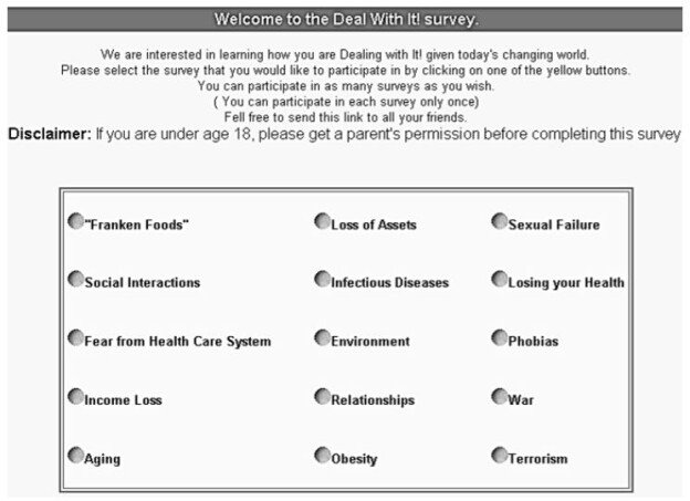
In 2003 the notion of expanding The It! studies to issues of anxiety emerged out of discussion among a group of researchers, viz., the author and colleagues [10,11]. The colleagues, Jacquelyn Beckley and Hollis Ashman of the Understanding and Insight Group in New Jersey drafted the first study, with its structure shown in Table 1 for obesity. Once the study had been constructed, it was straightforward to expand the topics to 14 other topics dealing with anxiety-provoking situations. Figure 1 shows the 15 studies, all ‘launched’ at the same time. The structure of the studies was maintained as much as possible, although as noted below, some of the elements had to be modified to accord with the study topic.
The remainder of this paper presents the study on obesity, was part of a set of 15 parallel studies called ‘Deal With It!’. We begin with the steps followed to set up the study, and move into a deep analysis of the results.
Table 1: The elements for the obesity ‘Deal With It!! Study. The left side shows the rationale for the element, the right side shows the specific language for the obesity study
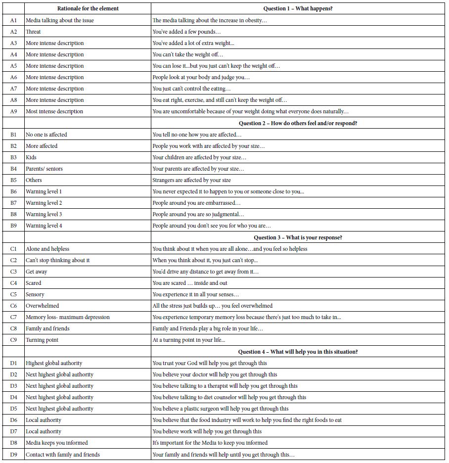

Figure 1: The 15 Deal with It! studies on a wall. The respondent chose the study she/he found interesting, and participated in that study
Step 1: Create the Elements to Describe One’s Personal Experience
The four sets of questions and nature of the answers were set up ahead of time. The structure on the left side of Table 1 was maintained for all 15 Deal With It! studies. The elements A1-A9, B1-B9, and some of the elements in Question 4 were different across the studies, to accord with the topic. The spirit of the answers were the same, but the specifics had to be modified to make sense. For the nine elements in Question C, the elements were far more similar to each other across studies, because there was no need to particularize the element to the topic.
The rationale for the elements was to make the language ‘vernacular,’ viz., informal. The motivation was to move away from a formal, possibly off-putting clinical presentation, and instead make the language informal, almost ‘folksy.’
Step 2: Create Vignettes – Mix Together Elements According to an Experimental Design
Mind Genomics differs profoundly in the way it measures the response to ideas, the messages shown in Table 1. Mind Genomics combines these messages in a systematized way to create vignettes, small, easy to read combinations of the messages. To the ordinary eye the combinations seen ‘haphazard,’ with the term ‘randomly put together’ often used to describe the 60 different combinations that would be evaluated by a single respondent. To that respondent, the combinations do seem random, but nothing could be further from the truth. The combinations are set up so that each combination or ‘’vignette’ comprises a minimum of two elements, a maximum of four elements, with all elements appearing an equal number of times across the 60 vignettes. Furthermore the 36 elements are statistically independent of each other, allowing the researcher to use programs like OLS (ordinary least-squares) regression to estimate how each element drives the ‘rating’ that the respondent is instructed to assign, after reading the vignette.
A further feature of the experimental design is that each respondent evaluates a unique set of 60 vignettes or combinations, so only in rare occasions do two respondents ever evaluate the same vignette. This novel approach, the so-called ‘permuted design’, acts metaphorically like the MRI, magnetic resonance imaging. With the MRI, the camera takes many X ray pictures of the underlying tissue, doing so from different angles, and afterwards combines them by computer to extract a 3-dimensional picture from a set of two-dimensional x-rays. Metaphorically, each respondent represents a different ‘angle’. The result is a deeper, more detailed view of the topic, because across the 107 respondents whose data are analyzed here, each respondent evaluating 60 different vignettes, we end up with 6420 different vignettes evaluated by the respondent. There is no need to ‘know the best combinations’ at the start of the study because the experimental design ensures that the researcher will sample a great deal of the underlying set of combinations [12].
It is important to emphasize that it is impossible to ‘game’ the Mind Genomics system. With a set of 60 vignettes, even the most dedicated effort will fail to uncover the pattern. As a consequence, the respondents stop trying to outwit the system, stop trying to give the ‘right answer’. Rather, they settle into an almost bored state, where they see something and they respond, pressing a key on the 9-point scale. As soon as the respondent pressed the rating scale the vignette disappeared, to be replaced by the next vignette. The rating scale, however, remained.
The instructions to the respondent were presented at the start of the study, the study executed on the computer. Figure 2 shows the standardized instructions, used for all 15 studies. The only thing which changed was the name of the study.
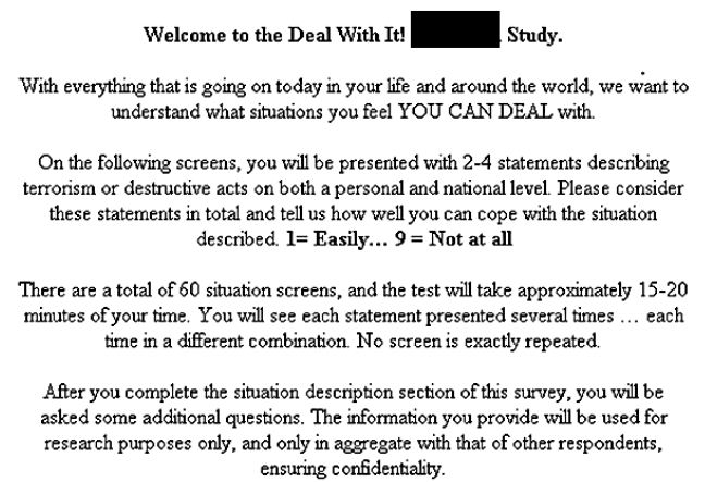
Figure 2: The orientation page, showing the topic (black rectangle), the rating scale, the expected length of time, and the reassurance that all vignettes are different
The actual vignettes were presented one at a time. As soon as the respondent assigned a rating the next vignette appeared. The 9-point rating scaling was always present on the screen, or at least appeared so as the on-line ‘experiment’ proceeded. In actuality, each vignette was totally new. The vignette comprised the elements at the top (in centered format, but without connectives). At the bottom of the screen was the refreshed rating scale.
By 2003, the year of the study, people were already accustomed to doing surveys on the Internet. The interview was described as a ‘survey’ rather than the more correct description, ‘experiment.’ The rationale was that the term ‘experiment’ might be off-putting and frightening.
The actual vignettes are described as situation screens, to which the respondents are asked to judge how she or he would react. No effort was made to measure the degree to which the respondent felt that the screen actually described them. That is, the respondent was treated as a disinterested judge, evaluating a situation or a scenario. In this way the appearance of an objective evaluation was maintained, even though the only criteria used by the respondent were her or his own point of view.
Finally, it is important to note that the introduction for each of the 15 studies was exactly the same, except for the topic. Thus, the top of the page welcomes the respondent, and gives the name of the study), where the black rectangle appears. For the obesity study the word was ‘obesity.’ The respondents are further told how long to expect the ‘survey’ to take (15-20 minutes), and that all the vignettes (screens) are different. This reassurance that ‘no screen is exactly repeated’ comes from the experience of respondents saying that they were sure they saw repeat screens, which of course they could not by virtue of the underlying experimental design.
Analysis
The Mind Genomics ‘process’ begins by transforming the ratings, bifurcating the original 9-Point Likert Scale into two regions. The rationale for this is that most users of the data end up asking ‘what does a certain value mean?’ This question can be asked of the original scale values (e.g., what does a rating of 8 mean on the scale), or it can be asked of the average rating across groups. Most peoples, including professionals, really do not understand the meanings of the different scale points. As a consequence of the widespread failure to understand what scale values really mean in everyday life, consumer researchers as well as public opinion pollsters have moved away from using Likert value data in reporting to using percentages, making their presentations easier to understand.
Following the aforementioned issues eventuated in Mind Genomics dividing the 9-point scale, almost arbitrarily, into ratings 1-6, coded 0, and ratings 7-9 coded 100. A vanishingly small random number is added to each of the transformed numbers, so that the binary ratings exhibit some random variation. That random variation will be necessary to avoid statistical issues when we deal with the individual-level modeling (viz., fitting equations to the data). The random variation will be so small, however, that there will be no effect on the data, other than avoiding the problem of having no variation in the ratings (viz., when a respondent assigns all vignettes either ratings 1-6, or ratings 7-9, which end up producing all 0’s or all 100’s as transformed values). The subsequent regression analysis cannot then be ‘run,’ and the analysis ‘crashes.’
The second step in Mind Genomics analysis creates an individual-level equation relating the presence/absence of the 36 elements to the binary response, 0/100, respectively. The aforementioned addition of the random variation to the transformed variable ensures that the regression analysis will always deal with data for which the dependent variable has ‘variation. The regression analysis is estimated using OLS (ordinary least squares) regression, a standard statistical analysis procedure. The regression generates the following equation: Binary Response = k0 + k1 (A1) + k2 (A2)… k36 (D9).
The data from all respondents generate a database. A total of 120 respondents participated. The data from 13 respondents were eliminated because their responses showed no variation at all. That is, all their ratings from 60 vignettes lay either between 1 and 6 (transformed to 0), or 7-9 (transformed to 100). Little can be learned from their reaction. This left 107 respondents who clearly discriminated among the elements, in terms of some elements driving anxiety, and the other elements not driving anxiety.
Summarizing the Data in an Easier Format
The aforementioned binary response equation generates a set of coefficients which show the likelihood that the specific element would drive a positive anxiety response, manifested by the rating 7-9 (‘cannot deal with it’, in the vernacular language of the rating scale). Negative coefficients mean that the element does not drive anxiety. Negative coefficients do not mean, however, that the element reduces anxiety. Quite the contrary. Negative coefficients simply mean that the element does not drive anxiety. The element may do absolutely nothing, or may reduce anxiety. We do not know. Our focus will be solely on the positive coefficients.
In the light of the meaning of the coefficient, our final transform is done on the coefficients themselves. All estimated coefficients for the 36 elements for each respondent, viz., k1-k36, were themselves rescaled. Coefficients of 8 or higher, corresponding to ‘cannot deal with it’ were transformed to 100. Coefficients of 7. 99 or lower, including 0 and negative coefficients, corresponding to elements which do not drive strong anxiety, were transformed to 0. The choice of ‘8’ as the cutoff comes from analyses of the regression modeling, which suggests that coefficients of 8 or higher are ‘statistically significant’, viz., the t statistic approaches 2.0. Furthermore, with coefficients of 8 (or more typically 10) or higher, one begins to see external behavior which confirms that the element or message is relevant for behavior.
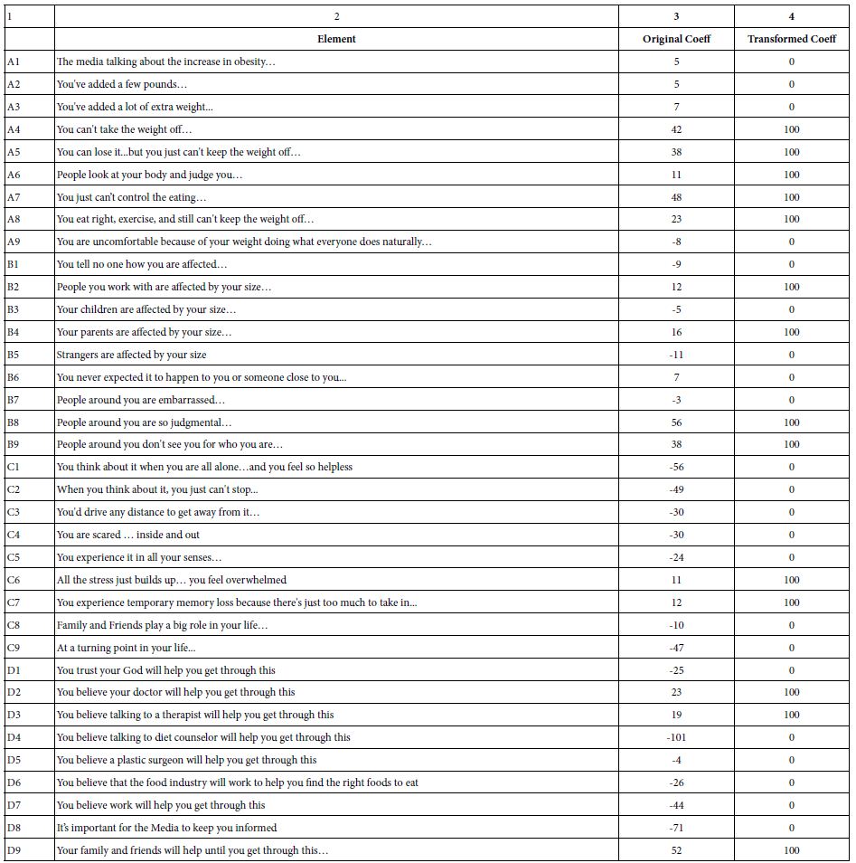
Table 2 shows an example of the 36 elements, (columns 1, 2), the coefficient emerging from the regression model (column 3), and the transformed coefficient (column 4). When we look at the data from total panel and key subgroups, this rescaling of coefficients will provide us with easy-to-understand averages, showing which elements drive anxiety and which do not.
Table 2: Example of the 36 estimated coefficients for two respondents (A, B, columns 3 and 4), their transformed value (columns 5 and 6). Coefficients of +8 or higher were transformed to 100. Coefficients lower than +8, whether positive, zero, or negative, were transformed to 0
What Drives Anxiety When Reading Vignettes about Obesity – Total Panel
Our first analysis (Table 3) presents the summary results for the total panel. The elements appear in column 1, with the element prefaced by an ‘X’ to remind us that the coefficients are transformed at the individual respondent level. Recall that a coefficient less than 8 is transformed to 0 at the level of the individual respondent, whereas a coefficient 8 or higher is transformed to 100.
Table 3: Average ‘transformed’ coefficients for the 36 elements. The transform replaced coefficients +8 or higher by 100, and coefficients less than +8 by 0. Note that the re-coded elements are prefaced by the letter X to signal the recoding the numbers represent the proportion of respondents who felt that they ‘could not deal’ with this situation described by the element, the proportion obtained by averaging the transformed coefficients
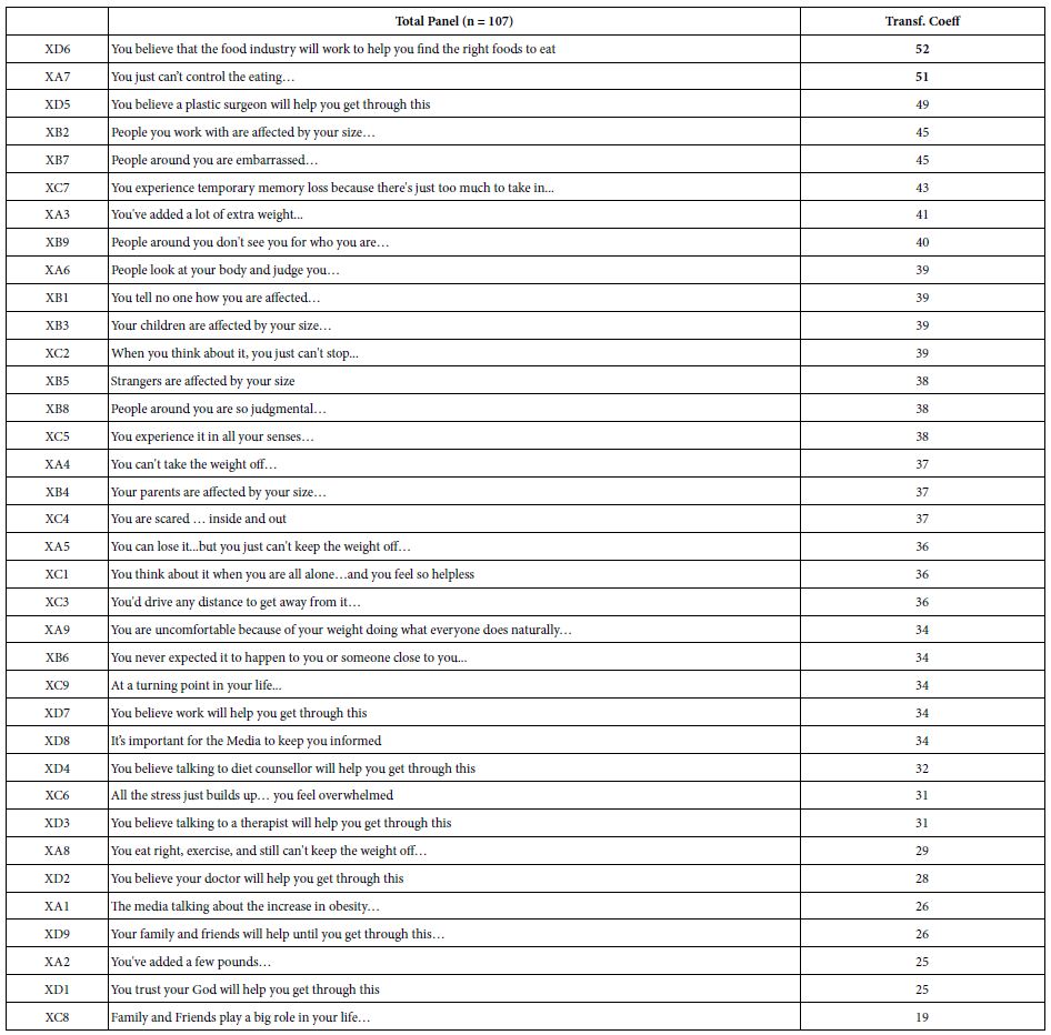
When we sort the 36 elements by the transformed coefficients, we see that 52% of the respondents will respond ‘I can’t deal with this’ when they are confronted with the statement that ‘You believe that the food industry will work to help you find the right foods to eat.’ Even though the phrase is stated in the positive, viz., that the food industry will help, the reality is that this statement is a negative. Slightly more than half of the respondents generate coefficients of +8 or higher.
Right below the panicked response to the stated ‘positive behavior of the food industry’ (!) are the statements ‘You just can’t control the eating…’ and ‘You believe a plastic surgeon will get you through this.’
It is important to reiterate that in a Mind Genomics study it is virtually impossible to ‘game’ the system. The elements are presented in different combinations, and each respondent evaluates what turns out to be most different combinations from everyone. Furthermore, the call on memory is so great that in these studies the respondents simply stop trying to be consistent, stop trying to outguess the researcher, and simply answer in a way that they feel is random, even though it is far from random. Thus the reactions we see in Table 3 represent the true feelings of the respondents, at least in 2003.
Delving Inside the Mind
After the respondent had completed the evaluation of the 60 vignettes, the respondent completed an extensive questionnaire about who the respondent was (gender, age, where live, income), the daily frequency that the respondent thought about ‘obesity’ (without any further explanation), how the respondent felt (select an emotion), where the respondent thought about the topic of obesity, and how the respondent was coping with the thought of obesity.
The next tables present partial, illustrative data, for several of these classification questions. Only data from subgroups of 10 or more respondents are shown, in the interest of both stability and cogency of analysis. The reality of a Mind Genomics study is the production of potentially hundred, sometimes thousands of data points. We present only strong coefficients, averages of 50 or higher. These are the elements to which at least 50% of the respondents react as driving an anxiety reaction (viz., rating of 7-9, cannot deal with it).
Time of Day When the Respondent Participated
The first classification question required the respondent to select the time of day that the respondent participated. The answers were presented as two-hour slots. The respondent selected the appropriate two-hour slot. The times were recoded to one of four periods during the day. The results are shown in Table 4.
Each cell in Table 4 tells us whether the element (row) covaries with anxiety (column), for at least 50% of the respondents. Empty cells in Table 4 correspond to elements and times wherein the average ‘transformed coefficient’ is less than 50.
Furthermore, in light of the 36 possible elements (rows), and the four times of day (columns), it is instructive to able to look at the elements from strongest to weakest as a driver of anxiety, and, in turn, look at the time of day as a driver of anxiety. Thus was born the strategy to sum up all the transformed coefficients (really sums of averages of transformed coefficients). Table 4 shows a row called ‘row sum’, and a column called ‘column sum’. These sums tell us which elements are the strongest across times of day (row sum), and which time of day is strongest across elements (column sum). We sort the table by row sum and column sum, presenting the data in descending order for both element (row sum), and for time of day (column sum).
Table 4: Average ‘transformed’ coefficients for the 36 elements, showing only strong performing elements for respondents based on the time of day in which they participated
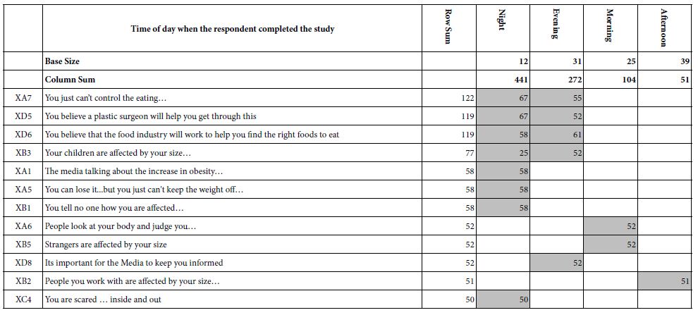
The sorting reveals that night, with a column sum of 441, is the most frequently selected period for an anxiety attack. The row sums suggest two elements are most anxiety producing across time of day: You just can’t control the eating; you believe a plastic surgeon will help you get through this; you believe that the food industry will work to help you find the right foods to eat.
Presenting the data in this transformed fashion (coefficients transformed to 0/100 and average), and creating/sorting by ‘sum’ produces a simple, clear picture of the relation between obesity (the topic), time of day, and type of message which creates anxiety. We create almost a 3-dimensional sense of the mind with respect to the topic, with the elements providing a rich, evocative language which provokes the reaction. Respondents simply need to participate in the study.
Frequency of Thinking about Obesity
Table 5 shows the strong performing elements for those who think frequently about obesity (5x or more per day), versus those who report that they think less frequently about obesity (0-4x per day). Keep in mind that these the numbers in Table 5 are average coefficients, and that only elements with coefficients of 50 or higher are shown.
Table 5: Average ‘transformed’ coefficients for the 36 elements, showing only strong performing elements for respondents based on the daily frequency of thinking about obesity
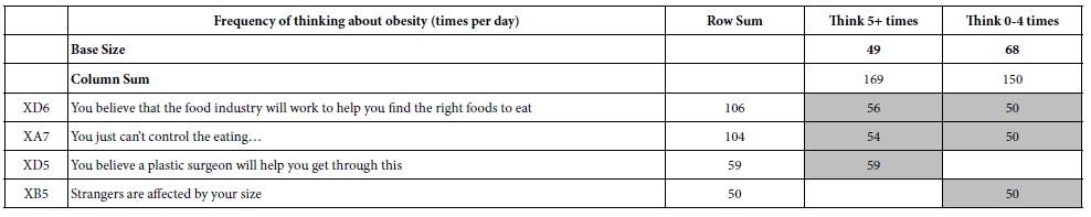
Those who think frequently about obesity respond most strong to the messages of plastic surgery (average transformed coefficient of 59, viz, 59% of the 49 respondents are responsive to this element). The other elements are the food industry, and the inability to control one’s eating. For those who think less frequently about obesity, the anxiety drivers are the food industry, and the lack of control.
Who the Respondent is – Age
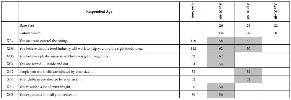
Moving the analysis to age (Table 6, again only for samples of 10+ respondents suggests that control is again a factor, but only for those age 41-60. For the younger respondents, ages 31-40, there are no elements which drive anxiety. For the older respondents, ages 41-60, control is again important. The two older age groups differ. Those age 41-50 respond to control. Those aged 51-60 respond to the mention of the plastic surgeon and the food industry, respectively. Furthermore, those aged 51-60 appear to be more attuned to themselves, and their behavior, acknowledging the fear.
Table 6: Average ‘transformed’ coefficients for the 36 elements, showing only strong performing elements for respondents based on 10-year age groups. Only respondent groups with at least 10 respondents in the group are shown
Who the Respondent is – Neighborhood
Researchers often think about issues of ‘geo-location’ as a key aspect to understand a person. Many studies ask the respondent to identify the city and state, or in some cases even ‘country’.’ The It! studies looked at location, but more in terms of the ‘neighborhood’ where the respondent lives, rather than the actual location.
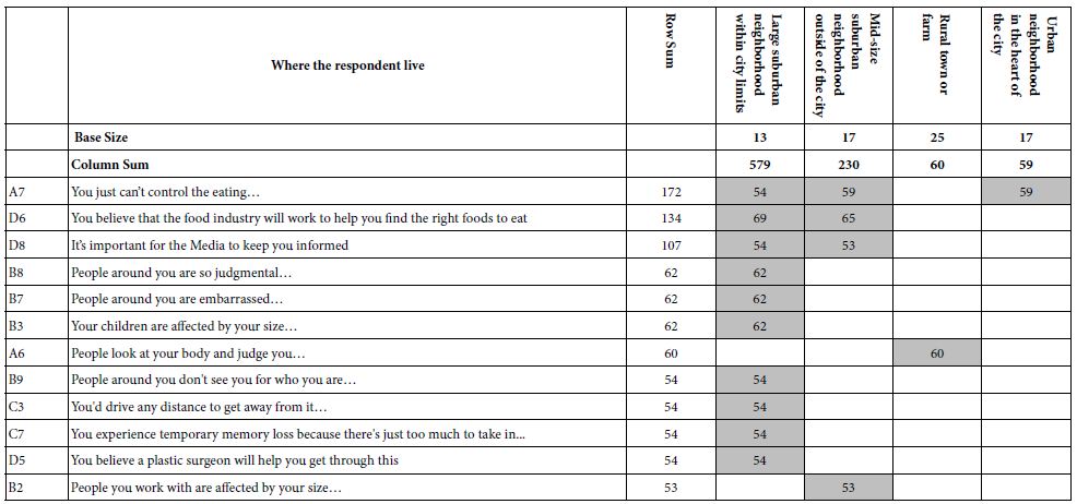
When we perform this new analysis, with transformed coefficients we find that those respondents who say they live in ‘large suburban neighborhoods within city limits’ are the ones with the greatest anxiety, manifesting itself in the strong reaction to the elements. Table 7 shows the strong performing elements, this time cutting off the elements at 53 to make the table easier to read. There were a number of elements around 50, but the pattern did not ‘tell a story,’ and so they are omitted from the table.
Table 7: Average ‘transformed’ coefficients, showing only strong performing elements for respondents based on the type of neighborhood where the respondent lives
Emotion Experienced at the End of the Evaluation
As part of the classification, the respondent was instructed to select up to three emotions experienced at the end of the evaluation. These were not emotions necessarily linked with the vignettes, but simply the selection of overall emotions after the evaluation of the 60 vignettes. Again, only emotions selected by 10 or more respondent were analyzed.
Table 8 shows the seven most frequently selected emotions, some positive, some negative. A surprising pattern emerges. The strong emotions (top left) emerge when the respondent selects the term ‘optimistic’ (sum = 463) and when the respondent selects the term ‘relaxed’ (sum = 452). The lowest sum of transformed elements occurs when the respondent selects the term ‘depressed’ (sum = 62).
Table 8: Average ‘transformed’ coefficients for the 36 elements, showing only strong performing elements for respondents based on the emotion selected by the respondent to how she or he felt at the end of the evaluation. The elements are sort by sums of strong performing elements
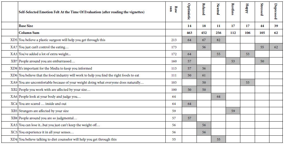
The strongest performing elements are those found on top. These are
You believe a plastic surgeon will help you get through this
You just can’t control the eating.
You’ve added a lot of extra weight.
People around you are embarrassed.
The only new element to appear is B7 (people around you are embarrassed). This element drives anxiety for three different types of respondents; optimistic, restless, and stressed, respectively. This element may be anomalous.
Location Where Anxiety is Experienced
The respondent was given a set of venues and instructed to identify up to three venues where the anxiety was experienced. Table 9 shows the most frequently selected with ‘at home’ being far and away the most frequent. Yet, in terms of the degree of anxiety, shown by the transformed coefficients, it was the more relaxed situations which covered with the greatest level of anxiety, such as listening to music, or talking with friend.
Table 9: Average ‘transformed’ coefficients for the 36 elements, showing only strong performing elements for respondents based on the self-profiling classification question dealing with the venue where anxiety was experienced. The elements are sorted by the sum of the strong performing elements
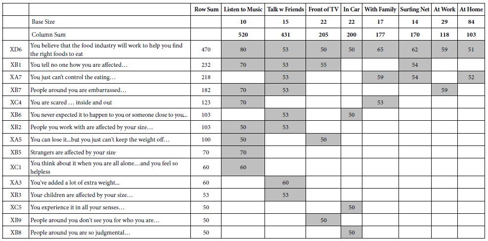
Finally, two other results deserve a short mention;
Those who said that they experienced the anxiety at home were most responsive to controlling their eating.
The pattern of strong performing elements once again shows the unexpectedly strong anxiety with regard to the food industry.
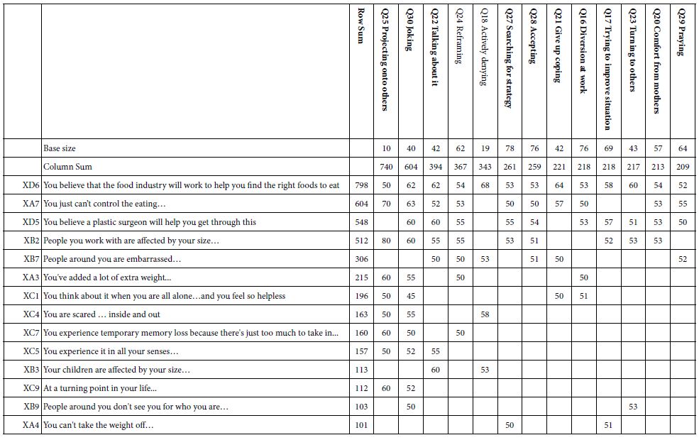
How Respondent Say They Cope with Their Anxiety
The final ‘major’ question on the self-classification portion, after the evaluation, was the presentation of different ways that a person could cope with anxiety. Each method of coping was separately rated on a 4-point scale, from 4=frequent to 1=never. For each method of coping, the analysis looked only at the respondents who rated that coping ‘4’ or ‘3’. Some method of coping (e.g., drinking alcohol) had very few respondents who said they hoped that way.
Table 10 shows the most frequent methods of coping, once again arranged in order of the sums of the coefficients of 50 or higher. The most surprising result is the ability of thinking about the food industry and obesity to cause a strong anxiety reaction.
Table 10: Average ‘transformed’ coefficients for the 36 elements, showing only strong performing elements for respondents based on the way the respondent states she or he copes with anxiety
Uncovering Mind-sets
A hallmark of Mind Genomics is the ability to uncover different mind-sets in the population, these mind-sets defined by how they respond to the test stimuli. Rather than dividing people by who they say they are, or what they say they do, or even dividing them by what they do, Mind Genomics divides them by the patterns of how they think about specific topics, such as obesity.
Each of the 107 respondents generated an individual vector of 36 coefficients. The pattern of coefficients in a sense tells us how the respondent ‘thinks’ about the topic, obesity, or at least how the respondent reacts after reading these vignettes, and what specific elements drive anxiety (viz., cannot deal with it).
Statisticians use cluster analysis to divide groups of objects into mutually exclusive and exhaustive sets, based upon the pattern of these objects. We have 107 respondents, our ‘objects.’ The patterns emerge from the vectors of 36 elements. The method of k-means cluster analysis places objects, viz our 107 respondents, into a limited set of non-overlapping groups Individuals with different looking patterns are put into different groups. There are many different ways to cluster respondents the method used here is called k-means [13]. With k-means clustering, respondents with similar patterns of 36 coefficients sre put into the same cluster (or mind-set, in the language of Mind Genomics).
K-Means uses a measure of distance between pairs of people, based upon the 36 coefficients. That measure is the value (1-Pearson Correlation). The Pearson Correlation tells us the strength of the linear relation between two objects, based upon two sets of corresponding measures, one for each object. When the relation between the two sets of 36 (non-transformed) coefficient is perfectly the Pearson correlation if +1 and the distance is 0 (1-1 = 0). When the relation is inverse, the Pearson correlation is -1, and the distance is 2 (1 – – 1 = 2).
When we apply the clustering approach to the coefficients, extracting either two mind-sets or three mind-sets the results become startling. Table 11 shows the strong performing elements. This time, however, it becomes far easier to label the mind=sets. Keep in mind that the clustering is done with the goal of extracting as few mind-sets as possible (parsimony), and the mind-sets telling a coherent story (interpretability).
Table 11: Average ‘transformed’ coefficients for the 36 elements, showing only strong performing elements for respondents. The respondents are assigned to one of two clusters (mind-sets, MS21, MS22) or separately one of three clusters (mind-sets, MS31, MS32, and MS33) based on k-means clustering
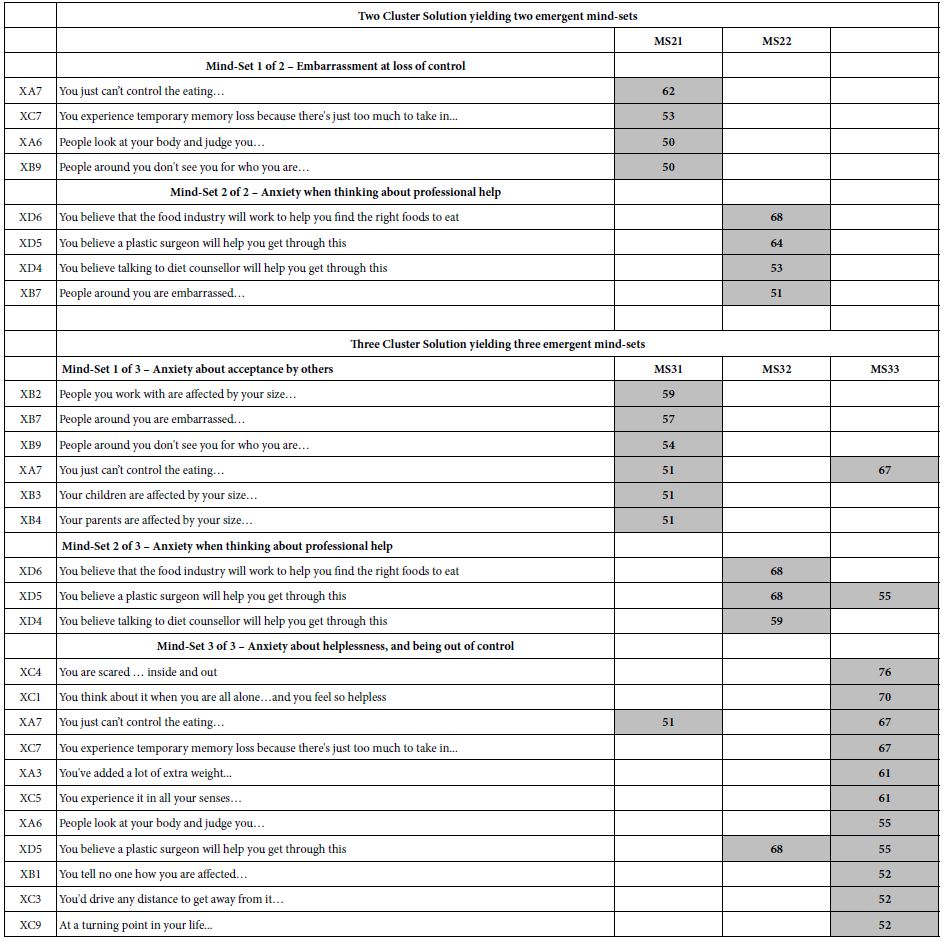
Conclusion
The focus of this paper has been on the response of people instructed to think about their responses if they found themselves to be obese. That is, the spirit of the paper is to understand how people think an obese person might react to different messages. Like the other 14 studies in the Deal It! series, the Obesity project was done with the general population, who were instructed to think about their responses if they suddenly found themselves in the situation of being obese.
The project was done with the general population. A minimum of information was obtained about the respondent, information relevant to who the respondent IS (geo-demos), and how the respondent might react in terms of the nature of the anxiety. No effort was made to measure the actual degree of obesity. The measurement of one’s BMI, had it been taken, could have been used as another way to classify the respondent, with the analyses then looking at low vs normal vs high BMI.
It is important to note that the structure of investigation in this paper follows the approach that consumer researchers use to evaluate the response to product ideas or product concepts. The idea or concept is explained to the respondent, either alone in a paragraph, or with a picture. The respondent, having read the idea and taking from the description a ‘sense’ of the product (or service), is then questioned about the reactions to the product, the expected benefits, expected problems, usage patterns, and even economic aspects such as the expected dollar value of the product.
Mind Genomics studies typically show differences among groups, these groups being defined by who the respondent is, and so forth. The largest differences, and indeed the most important ones, emerge out of the clustering of respondents into different groups, mind-sets, based upon the pattern of their responses to the test stimuli. The data presented here confirms the continuing finding that it is mind-sets, differences in the way people respondent to the same information, which produce the most meaningful results. Although there are some striking differences between groups in terms of the elements which drive strong anxiety reactions (viz., can’t deal with it, ratings of 7-9), the strongest and clearest differences emerge when we create heretofore unexpected groups of respondents using clustering procedures. The groups are remarkably different and easy to describe.
The important outcome of this first effort is a new ability to get a sense of how people feel, not so much from what they say as from the pattern of reactions to messages. By presenting the respondents with the vignettes, by estimating the individual-level coefficients, and then by transforming these coefficients into a binary form, we are afforded a quick way to understand what the sensitivity points are. The keys are the unexpected but anxiety-driving force of mentioning the food industry and the issue of self-control. These may have been obvious, but the Mind Genomics approach provides a degree of quantification, and the ability to put elements into the proper perspective based upon their performance in different groups
As a methodological advancement in understanding the way people respond to external stimuli (messages), Mind Genomics may provide a new direction. Hitherto, much of the work was based on clinical analyses, and tests of differences between obese and non-obese. Mind Genomics may well help create a new focus, namely how obese vs. non-obese react to the vernacular world, the world of everyday language and easy to understand ideas. In turn, this focus may energize new ways to teach the science of being healthy [14].
References
- Hockley RE (1979) Toward an understanding of the obese person. J Relig Health 18:120-131. [crossref]
- Barthomeuf L, Droit-Volet S and Rousset S (2009) Obesity and emotions: differentiation in emotions felt towards food between obese, overweight, and normal-weight adolescents. Food Qual Prefer 20: 62-68. [crossref]
- Ganley RM (1989) Emotion and eating in obesity: A review of the literature. Int J Eat Disord 8: 343-361. [crossref]
- Ogden J and Clementi C (2010) “The experience of being obese and the many consequences of stigma”. J Obes. [crossref]
- Moskowitz HR (2022) The perfect is simply not good enough: Fifty years of innovating in the world of traditional foods. Food Control 138:109626. [crossref]
- Moskowitz HR (2012) ‘Mind genomics’: The experimental, inductive science of the ordinary, and its application to aspects of food and feeding. Physiol Behav 107: 606-613. [crossref]
- Moskowitz HR, Gofman A, Beckley J and Ashman H (2006(a)). Founding a new science: Mind Genomics. J Sens Stud 21: 266-307. [crossref]
- Porretta S (2021) The changed paradigm of consumer science: from focus group to mind genomics. In Consumer-based New Product Development for the Food Industry. R Soc Chem. Pp: 21-39. [crossref]
- Harizi A, Trebicka B, Tartaraj A and Moskowitz H (2020) A mind genomics cartography of shopping behavior for food products during the COVID-19 pandemic. Eur J Med Nat Sci 4: 25-33. [crossref]
- Moskowitz MR, Ashman H, Minkus-McKenna D, Rabino S & Beckley JH (2006(b)) Databasing the shopper’s mind: approaches to a ‘mind genomics’. J Database Mark Cust Strategy Manag 13: 144-155.
- Rabino S, Moskowitz H, Katz R, Maier A, Paulus K, Aarts P, Beckley J, Ashman H (2007). Creating databases from cross‐national comparisons of food mind‐ J Sens Stud 22: 550-586. [crossref]
- Gofman A and Moskowitz H (2010) Isomorphic permuted experimental designs and their application in conjoint analysis. J Sens Stud 25: 127-145. [crossref]
- Likas A, Vlassis N and Verbeek JJ (2003) The global k-means clustering algorithm. Pattern Recognit 36: 451-461. [crossref]
- Losavio J and Gollub E (2022) Application of mindsets to health education and behavior change Programs. Health 14: 407-417. [crossref]


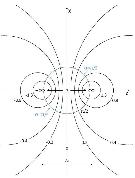
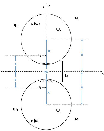

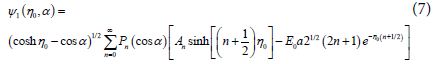
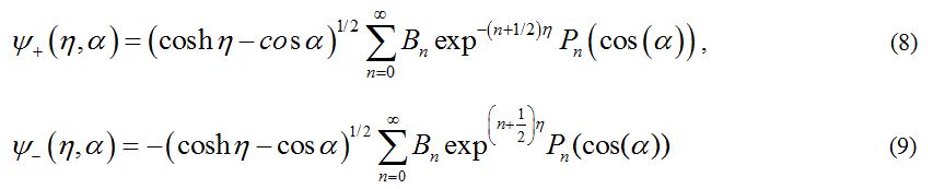
 is antisymmetric with respect to reflections through the xy plane i.e. Z → – Z or η → – η in agreement with the symmetry of the external electric field. The general solutions for the potentials in the surrounding medium, and in the upper sphere are given by Eqs (6) and (8), respectively. But the coefficients An and Bn should be obtained from the boundary conditions.
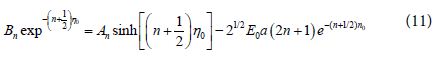
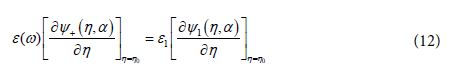
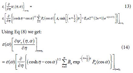
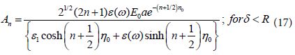
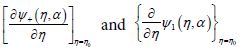 include the local plasmons charges induced on the surfaces of the spheres. In the present work we follow the idea, that for treating the limits of large field enhancement in hot spots we can use the following approximation which will simplify very much the analysis:
 represent more rapid decay of the local surface plasmons.
 into Eq (11) we get:
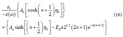
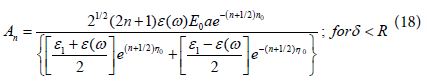
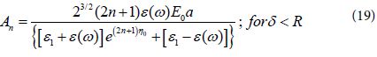
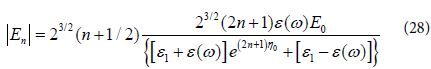
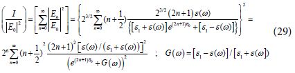
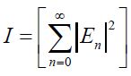 . Then the amplification of the light intensity at the center of the hot spots is given by: