Archives

fig 1a

Continuation of Temozolomide Chemotherapy in a Glioblastoma Patient After Resolution of COVID-19 Infection

DOI: 10.31038/CST.2022732

Abstract

We present a case of a 33 years old patient with glioblastoma who was diagnosed with Coronavirus disease 2019 (COVID-19) while undergoing chemotherapy. The patient did not have any other medical comorbidities. Due to active infection and leucopenia, his chemotherapy with temozolomide was on hold for 1 month. Temozolomide was resumed after resolution of leucopenia, improvement of COVID symptoms and a negative COVID-PCR (polymerase chain reaction) test. Patient continued to do well after administration of subsequent temozolomide cycles. A repeat computed tomography (CT) chest 2 months post infection revealed resolution of consolidation and no new areas of consolidation. Temozolomide was safely administered in this patient without reactivation of COVID-19 infection. Patient did not have any thrombotic events.

Keywords

Glioblastoma, COVID-19 pneumonia, Temozolomide, Chemotherapy resumption

Case Report

We present a case of a previously healthy 33 years old patient who presented with severe headaches and was found to have a right parietal lobe heterogeneously enhancing intra-axial neoplasm on magnetic resonance imaging (MRI) of the brain. He underwent a complete resection of the enhancing tumor volume. Pathology revealed a WHO grade IV astrocytoma, isocitrate dehydrogenase enzyme (IDH wild-type), O6-methylguanine-DNA methyltransferase (MGMT) unmethylated, positive CDKN2A loss (cyclin-dependent kinase inhibitor). He was subsequently treated as per the Stupp protocol with concurrent temozolomide and radiation followed by maintenance temozolomide. He was non-compliant with tumor treating fields which he self-discontinued after few months of treatment.

After completion of 3 out of 6 temozolomide cycles, he was admitted for fever and upper abdominal pain. A COVID-19 polymerase chain reaction (PCR) test was positive. He acquired this infection in the pre-COVID-19 vaccine era. Laboratory tests revealed normal WBC count of 4.8 K/UL, normal absolute neutrophil count (3.5 K/MM3), grade 2 lymphopenia with low absolute lymphocyte count (0.7 K/MM3). Computed tomography (CT) of the chest revealed patchy peripheral bibasilar ground glass and consolidative opacities compatible with pulmonary infection, with viral etiology such as COVID-19 (Figure 1A). He did not have pulmonary symptoms including shortness of breath or cough. Fever and abdominal pain resolved after 2 weeks of supportive care. However, due to the active COVID-19 infection and leucopenia, temozolomide dosing was held. It was subsequently resumed (cycle 4) after resolution of clinical symptoms and signs of COVID, normalization of hematological parameters (resolution of lymphopenia) and a negative COVID-19 PCR test. He tolerated his chemotherapy well through the completion of 6 cycles of temozolomide. A repeat CT chest 2 months after the initial COVID-19 infection revealed resolution of the lung consolidation (Figure 1B). Patient did not have any thrombotic events.

fig 1a

Figure 1A: Non contrast computed tomography chest showing bibasilar ground glass and consolidative opacities

fig 1b

Figure 1B: resolution of bibasilar ground glass and consolidative opacities after 2 months

Discussion

COVID-19, caused by the severe acute respiratory syndrome coronavirus 2 (SARS-CoV-2) which was declared as a global pandemic in March 2020 [1].

Impact of anti-cancer therapies on the course of COVID-19, and risk factors affecting the COVID-19 outcome for patients with primary brain tumors in particular, have not yet been elucidated. The aggravated immune response to COVID infection mediated by endothelial cells cytokines can potentially change the permeability of the blood brain barrier (BBB) causing exposure of the cerebral tissue to viral proteins [2].

Reactivation of virus post cancer chemotherapy has been reported with hepatitis B [3,4]. Similar concern exists with resumption of chemotherapy after SARS-CoV-2 infection. The immunocompromised state of cancer patients makes them more vulnerable to infection and morbidity with COVID-19 [5-7]. This increased vulnerability is partially due to the chronic immunocompromised state which can be exacerbated by anti-cancer therapies. There are conflicting results on risk of mortality with cytotoxic chemotherapy in COVID-19 patients [8-12]. Poor outcomes of COVID-19 infection in patients with receipt of recent chemotherapy is likely related to other comorbidities (peri-COVID-19 lymphopenia, neutropenia, diabetes, hypertension, and cardiovascular diseases) [10,13]. American Society of Clinical Oncology guidelines suggest waiting for infected patients to become asymptomatic and register a negative COVID-19 test before resuming treatment [9,14]. It is crucial to avoid under-treatment and treatment delays.

A report from the Dutch Oncology COVID-19 Consortium included 30 primary brain tumor patients of which 60% were glioblastomas [15]. Most patients had received cancer treatment ≤90 days prior to COVID-19 diagnosis. There were no indications of a negative impact of systemic anti-cancer therapies on the outcome of COVID-19 [15]. The thoracic cancer international COVID-19 collaboration (TERAVOLT) registry is the first large dataset of patients with COVID-19 and thoracic malignancies, regardless of therapies administered. No statistically significant association was found between anti-cancer treatment with mortality rate of the patients with thoracic cancers who were infected with COVID-19 [16]. Safe resumption of chemotherapy after resolution of COVID symptoms (approximately a month after the positive PCR test) has been reported in a young breast cancer patient without significant comorbidities [17]. There was no re-activation of COVID-19 or pulmonary adverse events [17]. Similarly, chemotherapy was safely resumed (approximately a month after the positive PCR test) in a 60 years old lady with ovarian cancer who was infected with COVID-19 [18]. In both these cases chemotherapy was resumed after resolution of COVID symptoms and negative PCR test. A 29 years old gentleman with a poor risk germ cell tumor safely resumed cytotoxic chemotherapy despite positive SARS-CoV-2 nasopharyngeal swab (he did have resolution of COVID symptoms) [19]. Two patients from Poland had no complications with chemotherapy continuation after COVID infection [20]. One patient was a young gentleman with primary mediastinal B-cell lymphoma, other patient was 56 years old gentleman with sigmoid cancer with asymptomatic COVID infection when receiving chemotherapy [20]. A prospective multi-institutional study 39 cancer patients in China reported low risk of SARS-CoV-2 reactivation after chemotherapy administration [21]. This study involved patients with different cancer pathologies including a 41 years old patient with glioblastoma with no comorbidities [21]. A severe case of COVID pneumonia was reported due to viral re-activation after resumption of immunosuppressive therapy (lymphocyte- and antibody-depleting therapy) in a 55 years old lady with CD20+ B cell acute lymphoblastic leukemia as well as other comorbidities including diabetes and cardiovascular disease [22]. Chemotherapy in her case was resumed 2 months after the first positive COVID PCR test, she had complete resolution of COVID symptoms and a negative PCR test before initiation of chemotherapy [22]. Most of the above studies indicate safe resumption of chemotherapy after resolution of COVID infection in patients without significant comorbidities.

For brain tumor patients there is lack of reliable data on the optimal timing and safety of resumption of cytotoxic chemotherapy in patients infected with COVID-19. Malignant gliomas are aggressive tumors with poor survival rates. Delay or discontinuation of cytotoxic chemotherapy will result in tumor progression and neurologic adverse events. Safety of adjuvant chemotherapy with temozolomide for treating gliomas during covid-19 pandemic has been reported [23]. Nevertheless, risk and benefits of chemotherapy should be considered especially in systemic chemotherapy such as alkylating agents, moderate delay in systemic treatment is acceptable [24]. To the best of our knowledge, there has been no report of continuation of chemotherapy with temozolomide in patients with high grade glioma and symptomatic covid-19 infection. In the case reported here, successful resumption of standard temozolomide dosing was possible with resolution of the COVID-19 associated clinical symptoms and radiographic findings and normalization of the hematological parameters. This report may provide insight into timing of safe resumption of essential chemotherapy post COVID-19 infection in a high grade glioma patient without significant comorbidities.

References

  1. Guan WJ, Ni ZY, Hu Y, Liang WH, Ou CQ, et al. (2020) Clinical Characteristics of Coronavirus Disease 2019 in China. N Engl J Med 382: 1708-1720.
  2. Ljubimov VA, Ramesh A, Davani S, Danielpour M, Breunig JJ, et al. (2022) Neurosurgery at the crossroads of immunology and nanotechnology. New reality in the COVID-19 pandemic. Adv Drug Deliv Rev 181: 114033. [crossref]
  3. Yeo W, Chan PK, Zhong S, Ho WM, Steinberg JL, et al. (2000) Frequency of hepatitis B virus reactivation in cancer patients undergoing cytotoxic chemotherapy: a prospective study of 626 patients with identification of risk factors. J Med Virol 62: 299-307. [crossref]
  4. Lubel JS, Angus PW (2010) Hepatitis B reactivation in patients receiving cytotoxic chemotherapy: diagnosis and management. J Gastroenterol Hepatol 25: 864-871. [crossref]
  5. Zhang L, Zhu F, Xie L, Wang C, Wang J, et al. (2020) Clinical characteristics of COVID-19-infected cancer patients: a retrospective case study in three hospitals within Wuhan, China. Ann Oncol 31: 894-901. [crossref]
  6. Zhang H, Han H, He T, Labbe KE, Hernandez AV, et al. (2021) Clinical Characteristics and Outcomes of COVID-19-Infected Cancer Patients: A Systematic Review and Meta-Analysis. J Natl Cancer Inst 113: 371-380. [crossref]
  7. Liang W, Guan W, Chen R, Wang W, Li J, et al. (2020) Cancer patients in SARS-CoV-2 infection: a nationwide analysis in China. Lancet Oncol 21: 335-337. [crossref]
  8. Cioffi R, Sabetta G, Rabaiotti E, Bergamini A, Bocciolone L, et al. (2021) Impact of COVID-19 on medical treatment patterns in gynecologic oncology: a MITO group survey. Int J Gynecol Cancer 31: 1363-1368. [crossref]
  9. Lievre A, Turpin A, Ray-Coquard I, Le Malicot K, Thariat J, et al. (2020) Risk factors for Coronavirus Disease 2019 (COVID-19) severity and mortality among solid cancer patients and impact of the disease on anticancer treatment: A French nationwide cohort study (GCO-002 CACOVID-19). Eur J Cancer 141: 62-81. [crossref]
  10. Tian J, Yuan X, Xiao J, Zhong Q, Yang C, et al. (2020) Clinical characteristics and risk factors associated with COVID-19 disease severity in patients with cancer in Wuhan, China: a multicentre, retrospective, cohort study. Lancet Oncol 21: 893-903.
  11. Yang K, Sheng Y, Huang C, Jin Y, Xiong N, et al. (2020) Clinical characteristics, outcomes, and risk factors for mortality in patients with cancer and COVID-19 in Hubei, China: a multicentre, retrospective, cohort study. Lancet Oncol 21: 904-913.
  12. Lee LY, Cazier JB, Angelis V, Arnold R, Bisht V, et al. (2020) COVID-19 mortality in patients with cancer on chemotherapy or other anticancer treatments: a prospective cohort study. Lancet 395: 1919-1926. [crossref]
  13. Jee J, Foote MB, Lumish M, Stonestrom AJ, Wills B, et al. (2020) Chemotherapy and COVID-19 Outcomes in Patients With Cancer. J Clin Oncol 38: 3538-3546. [crossref]
  14. ASCO, Cancer Treatment & Supportive Care.
  15. De Joode K, Taal W, Snijders TJ, Hanse M, Koekkoek JAF, et al. (2022) Patients with primary brain tumors and COVID-19: A report from the Dutch Oncology COVID-19 Consortium. Neuro Oncol 24: 326-328. [crossref]
  16. Garassino MC, Whisenant JG, Huang LC, Trama A, Torri V, et al. (2020) COVID-19 in patients with thoracic malignancies (TERAVOLT): first results of an international, registry-based, cohort study. Lancet Oncol 21: 914-922. [crossref]
  17. Horiguchi J, Nakashoji A, Kawahara N, Matsui A, Kinoshita T (2021) Chemotherapy resumption in breast cancer patient after COVID-19. Surg Case Rep 7: 170. [crossref]
  18. Liontos M, Kaparelou M, Karofylakis E, Kavatha D, Mentis A, et al. (2020) Chemotherapy resumption in ovarian cancer patient diagnosed with COVID-19. Gynecol Oncol Rep 33: 100615. [crossref]
  19. Pedrazzoli P, Rondonotti D, Cattrini C, Secondino S, Ravanini P, et al. (2021) Metastatic Mediastinal Germ-Cell Tumor and Concurrent COVID-19: When Chemotherapy Is Not Deferrable. Oncologist 26: e347-e349. [crossref]
  20. Wozniak K, Sachs W, Boguradzki P, Basak GW, Stec R (2021) Chemotherapy During Active SARS-CoV2 Infection: A Case Report and Review of the Literature. Front Oncol 11: 662211. [crossref]
  21. Bi J, Ma H, Zhang D, Huang J, Yang D, et al. (2020) Does chemotherapy reactivate SARS-CoV-2 in cancer patients recovered from prior COVID-19 infection? Eur Respir J 56: 2002672. [crossref]
  22. Lancman G, Mascarenhas J, Bar-Natan M (2020) Severe COVID-19 virus reactivation following treatment for B cell acute lymphoblastic leukemia. J Hematol Oncol 13: 131.
  23. Pessina F, Navarria P, Bellu L, Clerici E, Politi LS, et al. (2020) Treatment of patients with glioma during the COVID-19 pandemic: what we learned and what we take home for the future. Neurosurg Focus 49: E10. [crossref]
  24. Weller M, Preusser M (2020) How we treat patients with brain tumour during the COVID-19 pandemic. ESMO Open 4: e000789. [crossref]
fig 3

A Study to Assess Outcome of Hip Fractures in Elderly Patients with Associated Hyponatraemia and Review of Literature

DOI: 10.31038/IJOT.2022513

Abstract

Introduction: Hyponatremia is a clinical condition which can be summarized when serum sodium is less than 135 mMol/L, it is the most commonly encountered electrolyte imbalance in clinical practice. It is usually associated with poor clinical outcomes including falls, fractures, increased length of hospital stay, institutionalisation and mortality. Prevalence is known to increase in frail patient groups, such as elderly, hospitalised, peri-operative patients with a fracture. Elderly patients with fragility fractures (EPFF) have increased risk of hyponatremia as a result of degenerate physiology, multiple co-morbidities, polypharmacy, increased risk of dehydration due to hospitalisation and peri-operative fluid restriction, and homeostatic stress from fracture and subsequent surgical interventions.

Material and Method: We conducted a prospective interventional study in a tertiary care centre including 43 patients above the age of 60 years (Range 61 years to 90 years) (Mean age 71.23 years) admitted with fragility fracture around hip, which included inter-trochanteric fractures, sub-trochanteric fractures and neck of femur fractures, pubic ramus fracture, mode of trauma strictly being low energy injuries like trivial fall, patients with high energy trauma, and injuries like shaft of femur fracture, acetabular fracture, pelvic ring fractures were excluded from the study.

Results: Amongst 43 patients incidental hyponatraemia was seen in 36(83.72%), with mild (41.86%), moderate (27.90%) and severe (13.95%), incidence of diabetes mellites type 2 was seen in (74.41%), hypertension was (83.72%), chronic kidney disease upto stage 2 was seen in (6.9%) and (18.6%) were hypothyroid, there were (n=13) patients whose comorbidities were noticed after injury. Average duration of hospital stay and Barthel index (scale to measure activity of daily living) showed linear correlation with initial stage of hyponatraemia in patients, with length of hospital stay was average 24.75 days among the severe deficiency group and 15.25 days in normonatremic group, Barthel index was (90 to 100) among the normonatremic patients and less than 70 in patients with initial hyponatremia at 2 weeks from surgery.

Conclusion: With our study we can conclude that we have to look out for electrolyte disturbance, sodium being most common, incidence of fragility fractures with sodium disturbance, can be due to manifestation of osteoporosis, early diagnosis and management can help in preventing as well as in good outcome in such injuries.

Introduction

Hyponatremia is a clinical condition which can be summarized when serum sodium is less than 135 mMol/L, it is the most commonly encountered electrolyte imbalance in clinical practice [1,2]. It is usually associated with poor clinical outcomes including falls, fractures, increased length of hospital stay, institutionalisation and mortality [3]. Prevalence is known to increase in frail patient groups, such as elderly, hospitalised, peri-operative patients with a fracture. Elderly patients with fragility fractures (EPFF) have increased risk of hyponatremia as a result of degenerate physiology, multiple co-morbidities, polypharmacy, increased risk of dehydration due to hospitalisation and peri-operative fluid restriction, and homeostatic stress from fracture and subsequent surgical interventions [5]. They are also at higher risk of complications, making this group of special clinical importance. Hyponatremia itself may be responsible for the fracture. Reports of the prevalence of hyponatremia at admission in EPFF vary widely between 2.8%-26.5%, while 2.6-5.5% develop hyponatremia in the post-operative period. Hyponatremia occurs due to disruption of sodium and water homeostasis, normally maintained by complex multi-system physiological mechanisms. Consequently, there are numerous potential underlying causes of hyponatremia, spanning a broad spectrum of diseases, pharmacotherapy and pathophysiological variants each with different treatment requirements. When very acute or severe, hyponatremia may present with neurological symptoms which can result in serious complications e.g. hyponatraemic encephalopathy, non-cardiogenic pulmonary oedema, seizures, coma, death. However, 75-80% of cases of hyponatremia are mild and chronic (i.e. serum sodium 130-134 mMol/L, occurring over 24 hours) and typically devoid of obvious neurological symptoms [6]. As a result, chronic mild hyponatremia is frequently considered asymptomatic despite being strongly associated with major geriatric conditions and multi-organ pathological changes. These include abnormal gait patterns, falls, fractures, cognitive impairment, bone demineralisation, longer hospital stay, institutionalisation and increased mortality [7]. Despite this, older people may be at lower risk of hyponatraemic encephalopathy and subsequent complications of acute severe hyponatremia, where female gender, hypoxia and liver dysfunction are associated with poorer prognosis [8] whether hyponatremia is an independent predictor of patient outcomes or a marker of disease severity is controversial [9]. Nevertheless, it is very treatable, so its association with multiple poor clinical outcomes is important.

Materials and Methods

We carried out a prospective observational study of all adults aged 65 years or over admitted with a fragility fracture to a university teaching hospital from 7th January – 4th April 2021. Fragility fractures were defined as those occurring either without trauma or due to low energy trauma, equivalent to a fall from standing height or less than one metre. Anonymous baseline data (age, sex, fracture site and admission serum sodium) of all identified EPFF were recorded (Tables 1 and 2).

Table 1: Patient range

Age range

Number of patients

65-70

9

71-75

8

76-80

10

81-85

8

86-90

5

Above 90

3

Total

43

Table 2: Patients and Serum Na levels

Serum Na level at the time of admission

Number of patients Serum Na after administration of correction Serum Na at the time of discharge from hospital

Mean hospital stay from date of admission in days

135-145

7

Nil given >135-140

15.25

131-135

18

>136-140 >135-140

18.25

126-130

12

>130 >135

23.55

121-125

6

>130 >135

24.75

Inclusion Criteria

We included patients with age more than or equal to 65 years, patients who gave history of trivial trauma, like fall due to slipping of foot, who didn’t gave any history of direct trauma, patients with trauma around hip, so fractures included were inter-trochanteric, sub-trochanteric, pubic ramus fractures also we included neck of femur fractures, patients with medical comorbidities were included and their baseline investigations were done.

Exclusion Criteria

Adults with incapacity were excluded from recruitment and those associated with head injury or any other systemic trauma and with mode of trauma which included high velocity were also excluded. Patients with trauma which required prolonged bed rest were also excluded. Those with any history of metastatic illness were excluded. Participants were recruited from acute orthopaedic trauma wards and a geriatric assessment unit. Clinical data were collected daily until discharge, from patient interview, medical and nursing notes, observation and fluid balance charts and laboratory computer systems by a single investigator. Medication data were obtained by reconciling patient and/or carer histories, and primary and secondary care records. Also, clinical examination of volemic status was performed daily by the investigator. This involved measurement of skin turgor, capillary refill time, mouth moistness, axillary moistness, jugular venous distension, peripheral oedema and overall impression (signs selected based on previous research recommendations) [22]. Examination was carried out by one investigator to increase reliability of findings, maximise consistency and exclude effects of inter-observer variability. Cases of hyponatremia were defined as any serum sodium measurement, 135 mmol/L. An expert panel, consisting of two consultant geriatricians with special interest in hyponatremia and one consultant orthopaedic surgeon reviewed and determined aetiology of each case of hyponatremia. The panel did not examine patients themselves but instead retrospectively reviewed each case of hyponatremia relying on the detailed daily prospectively collected data and clinical examination findings provided by the investigator. This included all clinical information required to determine underlying cause(s) of hyponatremia – history, medications, detailed daily examination, fluid intake and output charts and laboratory results. Collectively, the expert panel used a diagnostic algorithm to determine underlying cause(s) of hyponatremia. The prevalence of hyponatremia upon admission and the incidence of cases developing in hospital were calculated. For incident cases, we recorded whether the hyponatremia was pre- or post-operative. The proportion of participants with known hyponatremia prior to their fracture was calculated by obtaining the last available serum sodium for each patient prior to their admission to hospital. The laboratory is the only public health service laboratory covering the study population so it was unlikely that patients had more recent investigations elsewhere. Prevalence of hyponatremia at discharge was calculated according to the last available serum sodium measurement prior to discharge (Figures 1 and 2).

fig 1

Figure 1: Barthel index of activities of daily living

fig 2

Figure 2: Interpretation of scoring on the Barthel index

Observation and Results

After Recruitment, participant information and data collection there were 167 patients with fragility fractures who presented to our hospital during that period, many of the patients had upper limb fracture mostly dominated by distal radius fracture, after applying our inclusion and exclusion criteria we included total 43 patients in our study. Those not recruited had incapacity to consent, declined participation, or agreed but were later excluded when the original diagnosis of fragility fracture was excluded. There were no statistically significant differences between participants and those who were eligible but declined participation. Amongst the patients we had 43 patients in all, with inter-trochanteric fractures in 10 patients, subtrochanteric fracture in 12 patients and neck of femur fracture in 18 patients and pubic ramus fractures in 3 patients, and among the associated co-morbidities diabetes mellitus type 2 was seen in (74.41%) patients and hypertension in (83.72%) chronic kidney disease upto stage 2 (6.91%) and hypothyroid was seen in (18.6%). Among all the Patients with associated comorbidities who were discovered at the time of admission, and so were not on any medication were total n=13(30.23%). Barthel index for daily activities was noted at the time of dmission, during hospital stay and time of discharge. We noticed we had 7 out of 43 patients who were normo-natremia, 18 patients had mild and 12 mad moderate and 6 had severe hyponatraemia, patients with severe hyponatraemia also had confusion and weakness during peri-traumatic period, and many scholarly articles also have published similar complaints, which was due to hyponatraemia. We noticed that patients with severe hyponatraemia at the time of presentation had mean hospital stay of 24.75 days and those with normo-natremia had mean hospital stay of 15.25 days, there was also similar observation in recovery of the patients with normo-natremia patients having a gradual and sustained increase in Barthel index, due to early mobilisation and shorter duration in trauma to surgery interval with mean od 4.3 days for surgery from trauma and 6.5 days for patients with deranged serum Na levels, for which correction was administered as per general medicine and nephrologist opinion, after serum Na correction there improvement in general condition as well as tolerance to physiotherapy post-surgery. Barthel index was (90 to 100) among the normonatremic patients and less than 70 in patients with initial hyponatremia at 2 weeks from surgery (Figures 3 and 4).

fig 3

Figure 3: Symptoms

fig 4

Figure 4: Chronic Hyponatremia

Discussion

We found that, compared to men with serum sodium ≥135 mmol/L men with serum sodium values <135 mmol/L had approximately a 3 fold increase in the risk of hip and incident morphometric spine fractures and a 2½ fold increase in the risk of prevalent morphometric spine fractures. Further, the strength of the relationship between hyponatremia and fractures was not substantially reduced after adjusting for multiple well established fracture risk factors, and in particular, for falls and bone mineral density [10].

Our results are consistent with previous studies that have reported on associations between hyponatremia and fractures. A case control study identified 513 cases of fractures (mainly hip and femoral neck) after a fall and reported an increased risk of fracture, by about 3 fold in men and women with hyponatremia (<135 mmol/L)[11], even after adjusting for medications and medical conditions known to confound that association between fracture and serum sodium. A second case control study reported on the prevalence of hyponatremia (<135 mmol/L) among 364 subjects presenting to the emergency department with fractures of the hip/pelvis and femur compared with the incidence of hyponatremia in 364 controls (subjects presenting to the emergency department with non-critical complaints)[12]. The incidence of hyponatremia in those with fractures was more than double that of controls. A recent cross sectional study by Arampatzis et al. reported that of 10,823 emergency department admissions among adults (≥50 years) there was an increased risk of osteoporotic fracture (OR= 1.46; 95%CI: 1.05 to 2.04) among individuals with diuretic-induced hyponatremia. A secondary data analysis of 1408 women participating in a study of chronic kidney disease determined that those with hyponatremia (again less than 135 mmol/L) had a 2 fold increase risk of fracture (based on self-report) even after adjusting for BMD [13,14].

Our analyses showed similar but generally stronger associations between hyponatremia and fracture risk compared to the only other prospective study of the issue; a secondary analysis performed within the Rotterdam Study that included 5208 men and women of which 399 (9%) had a hyponatremia (serum sodium <135 mmol/L)[15]. In the Rotterdam Study those with hyponatremia there was a 1.4 fold increase in nonvertebral fractures over 7.4 years of follow up and a 1.8 fold increase in prevalent but not incident vertebral fractures or hip fractures. As in our study, adjustment for factors such as disability index and falls did not substantially change the results. Of note, BMD was not associated with low serum sodium in the Rotterdam cohort [16,17].

There are several mechanisms by which low serum sodium might contribute to an increase risk of fracture. Hyponatremia, even when mild as in our study, might increase the risk of falls and fall related fractures by causing gait instability and attention deficits. One study reported that the threshold for gait deficits associated with hyponatremia was 134 mmol/L and 132 mmol/L for attention deficits. In our study we noted that 31% of men with hyponatremia reported falls in the past 12 months compared with 21% of men with serum sodium >135 mmol/L. However, adjusting for baseline fall history did not substantially change the relationship between hyponatremia and fracture.

There is growing evidence to suggest that unrecognized complications of hyponatremia include bone loss and osteoporosis, though the mechanisms by which this occurs is not clear. Cellular and animal data suggest that hyponatremia may have a direct effect on bone. Hyponatremia can directly stimulate osteoclast genesis and osteoclastic resorption without activation of signalling through osteoblasts [18,19]. Finally, it is possible that hyponatremia is a surrogate marker for other causes of fracture. In our study as well as in others, subjects with hyponatremia were older, in poorer health, more likely to report use of relevant medications (such as diuretics, SSRI’s) and have concomitant illnesses such as thyroid disease that increase the risk of fractures. However, in our analyses the associations between hyponatremia and fracture risk was not substantially altered by adjusting for many potential confounding factors including falls suggesting that hyponatremia might be associated with bone quality. Thus, assessment of BMD with DXA in mild hyponatraemic subjects may not represent the best available method to address microstructural skeletal alterations [20].

Our study had some limitations. Most importantly, this was not a randomized trial and as such it is not possible to definitively conclude that low serum sodium causes fractures, and that correcting serum sodium will reduce the risk of fractures. Another limitation of our study was the fact that serum sodium was measured only at baseline.

Our findings suggest that hyponatremia, one of the most common electrolyte abnormalities, is associated with up to a doubling in the risk of hip and morphometric spine fractures. The association we observed was strong despite the low prevalence of hyponatremia in our cohort and was not altered by adjusting for fall history or bone mineral density. Further studies are needed to determine if hyponatremia results in an increase in fractures, the mechanism by which this occurs, and whether treatment of hyponatremia reduces the incidence of fractures.

Conclusion

With our study we can conclude that we have to look out for electrolyte disturbance, sodium being most common, incidence of fragility fractures with sodium disturbance, can be due to manifestation of osteoporosis, early diagnosis and management can help in preventing as well as in good outcome in such injuries. From our study we can also draw a relationship between, hyponatraemia and osteoporosis and also weakness and associated confusion in severe hyponatraemia, though our study is limited with a exclusion of upper limb fragility fracture and also vertebral osteoporotic fractures, we can successfully draw a conclusion regarding early electrolyte restoration post trauma and also a scrutiny in suspected patients for early detection and prevention of such fractures.

References

  1. Gankam KF, Andres C, Sattar L, Melot C, Decaux G (2008). Mild hyponatremia and risk of fracture in the ambulatory elderly. 101: 583-588 [crossref]
  2. Tolouian R, Alhamad T, Farazmand M, Mulla ZD (2012). The correlation of hip fracture and hyponatremia in the elderly. J Nephrol 25: 789-793. [crossref]
  3. Sandhu HS, Gilles E, DeVita MV, Panagopoulos G, Michelis MF (2009). Hyponatremia associated with large-bone fracture in elderly patients. Int Urol Nephrol 41: 733-737.
  4. Arampatzis S, Gaetcke LM, Funk GC, et al. (2013). Diuretic-induced hyponatremia and osteoporotic fractures in patients admitted to the emergency department. Maturitas 75: 81-86. [crossref]
  5. Kinsella S, Moran S, Sullivan MO, Molloy MG, Eustace JA (2013). Hyponatremia independent of osteoporosis is associated with fracture occurrence. Clin J Am Soc Nephrol 5: 275-280. [crossref]
  6. Hoorn EJ, Rivadeneira F, van Meurs JB, et al. (2011). Mild hyponatremia as a risk factor for fractures: the Rotterdam Study. J Bone Miner Res 26: 1822-1828. [crossref]
  7. Blank JB, Cawthon PM, Carrion-Petersen ML, et al. (2005) Overview of recruitment for the osteoporotic fractures in men study (MrOS). Contemporary clinical trials.26: 557-568. [crossref]
  8. Orwoll E, Blank JB, Barrett-Connor E, et al. (2005) Design and baseline characteristics of the osteoporotic fractures in men (MrOS) study–a large observational study of the determinants of fracture in older men. Contemp Clin Trials 26: 569-58. [crossref]
  9. Cauley JA, Blackwell T, Zmuda JM, et al. (2012) Correlates of trabecular and cortical volumetric bone mineral density at the femoral neck and lumbar spine: the osteoporotic fractures in men study (MrOS). J Bone Miner Res 25: 1958-1971. [crossref]
  10. Genant HK, Wu CY, van Kuijk C, Nevitt MC (1993) Vertebral fracture assessment using a semiquantitative technique. J Bone Miner Res 8: 1137-1148. [crossref]
  11. Mackey DC, Lui LY, Cawthon PM, et al. (2007) High-trauma fractures and low bone mineral density in older women and men. JAMA 298: 2381-2388. [crossref]
  12. Pahor M, Chrischilles EA, Guralnik JM, Brown SL, Wallace RB, et al. (1994) Drug data coding and analysis in epidemiologic studies. Eur J Epidemiol 10: 405-411. [crossref]
  13. Bailey IL, Lovie JE (1976) New design principles for visual acuity letter charts. Am J Optom Physiol Opt 53: 740-745. [crossref]
  14. Levey AS, Stevens LA, Schmid CH, et al. (2009). A new equation to estimate glomerular filtration rate. Ann Intern Med 150: 604-612. [crossref]
  15. Renneboog B, Musch W, Vandemergel X, Manto MU, Decaux G (2006) Mild chronic hyponatremia is associated with falls, unsteadiness, and attention deficits. Am J Med 119: 7. [crossref]
  16. Barsony J, Sugimura Y, Verbalis JG (2011) Osteoclast response to low extracellular sodium and the mechanism of hyponatremia-induced bone loss. J Biol Chem 286: 10864-75. [crossref]
  17. Verbalis JG, Barsony J, Sugimura Y, et al. (2010) Hyponatremia-induced osteoporosis. J Bone Miner Res 25: 554-563. [crossref]
  18. Hoorn EJ, Liamis G, Zietse R, Zillikens MC (2011) Hyponatremia and bone: an emerging relationship. Nat Rev Endocrinol 8: 33-39. [crossref]
  19. Lindner G, Pfortmuller CA, Leichtle AB, Fiedler GM, Exadaktylos AK (2014) Age-related variety in electrolyte levels and prevalence of dysnatremias and dyskalemias in patients presenting to the emergency department. Gerontology 60: 420-423. [crossref]
  20. Adrogue HJ, Madias NE (2000) Hyponatremia. N Engl J Med 342: 1581-1589.
fig 3

Case Report of Surgical Treatment of Spiral Fracture of Medial Femoral Condyle by ORIF Using Lag Screws and Posterior Buttress Tibial Plate in Elderly Lady and Review of Literature

DOI: 10.31038/IJOT.2022512

Abstract

Introduction: Fractures of medial condyle of femur are typically rare here we report a case of medial femoral condyle fracture with multiplanar displacement treated with cortico-cancellous screw for compression and posterior tibial plate used as an anti-glide plate/buttress for oblique/spiral configuration of fracture.

Case Presentation: A 78-year-old woman sustained trauma due to fall from stairs and was brought to our hospital with severe right knee pain and inability to bear weight and walk. Knee radiographs (Figure 1) revealed right femoral medial fracture in spiral configuration extending into intercondylar notch as well as breaking in posterior cortex. It is classified (AO classification 33-B2) Patient was initially stabilised and immobilised in splintage. All pre anaesthetic investigations performed and patient was planned for open reduction internal fixation. ORIF was done using two 6.5 mm partially threaded cancellous lag screws to compress the condyle and posteriorly extending oblique pattern of fracture compressed by proximal tibia posterior plate as anti-glide plate. The patient had uneventful post-operative recovery and recent follow up patient achieved a range of motion of zero to 120 degree and could walk without pain.

Conclusion: The locking compression plate for proximal tibia can be used solution for difficult femoral condyle fracture used in reversed position. However careful patient selection is important.

Introduction

Distal femur fractures account for 7% of all femur fractures if hip fractures are excluded then one third of femur fractures involve the distal portion [1], a bimodal age distribution exists with high incidence in young males due to high energy trauma such as motor vehicle or motorcycle accidents or fall from heights a second peak in elderly woman from minor falls there is ratio of 1:2 in men to women [1,2]. Femoral medial condyle fracture (AO classification 33-B2) is a considerably rare fracture. Limited literature is available to give clear view regarding treatment of this fracture configuration. Being metaphyseal region and intra-articular extension, anatomical reduction, and compression as well as stable fixation is a primary necessity to achieve better functional outcome [3]. However, in this case the spiral fracture pattern in distal femur metaphysic the fracture line itself has extended into two planes, Proximal fracture pattern was in coronal orientation and distal in sagittal plane. Hence compression could only have been achieved when screws are placed in the tangential plane to the plane of fracture line. Proximal end of the fracture being smaller in dimension to accommodate the lag screw. However, this compression in other plane could not be achieved through single plane orientation of the plate hence needs isolated another fixation modality. The plate must be precontoured to match posterior surface of distal femur to offer adequate compression till healing and combination construct was needed to be used. Considering the vertical line of fractures and the obliquity of the displacement, screw fixation compression can be done but to achieve stability however no current anatomical plates fit the femoral medial condyle [4,5]. We present a case of femoral medial condyle fracture treated with cancellous screws and posterior tibial plate used as anti-glide plate/buttress plate.

Case Presentation

A 78-year-old woman was brought to our hospital after sustaining trauma to her right knee due to fall from stairs. She was not suffering from chronic neurological illnesses. Parkinson’s disease or stroke or paralysis any signs of central nervous dysfunction or paralyses, all her vital signs were normal. On evaluation patient complained of pain and inability to move right lower limb, there was swelling and bruising over the knee, tenderness was elicited on palpation, distal neurology and vascularity were intact radiographs was done which demonstrated (Figure 1) a femoral medial condyle fracture of right side, the fracture was intra articular and simple oblique through the intercondylar notch (AO classification 33-B2) patient was admitted to our hospital for open reduction internal fixation to be performed following day after stabilization.

fig 1

Figure 1: radiograph done at time of presentation

Surgical Procedure

Patient was planned for open reduction and internal fixation, under all aseptic conditions, spinal and epidural anaesthesia, fixation patient was performed in supine position. Medial subvastus approach (Figure 2) was used, this approach is used for intra articular fractures of medial condyle of femur, medial Hoffa or in addition to lateral parapatellar approach in case of severe bicondylar articular fragmentation, a skin incision was started at the adductor tubercle and extends proximally just posterior to vastus medialis and the interval between vastus medialis and sartorius was identified, vastus medialis was elevated to expose the medial femoral condyle (Figure 2) the popliteal vascular bundle was protected which lies between adductor Magnus and intermuscular septum.

fig 2

Figure 2: intra-operative images

The fracture was initially compressed with cortico-cancellous screw in coronal plane (Figure 3) and a lag screw was passed to compress the fracture in sagittal plane and then posterior tibial plate was used upside down to fit the Bony surface, the plate was bent for achieving proper anatomical orientation and fixed with cortical and locking screws thus the plate was used as anti-glide/Buttress as per the configuration of the fracture, closure was done in layers. Patient had uneventful post-operative recovery, range of motion exercises were started on Day 1, the weight bearing protocol was toe touch gate for first 4 weeks, by 4th week partial weight bearing from 6 weeks half partial weight bearing and from eight weeks full weight bearing, at the latest follow up the patient had range of motion of zero to 120 degree without any pain, she could walk freely and joint surface restoration was maintained radiologically (Figure 4).

fig 3

Figure 3: Range of motion after 6 months of surgery

fig 4

Figure 4: follow up radiograph

Discussion

In elderly patients with osteoporosis a low energy trauma causes simple spiral or oblique fractures the shape of distal femur when viewed end on is a trapezoid with posterior part wide then the anterior part creating 25 degree of inclination on the middle surface and about 10 degree on the lateral surface the plate should lie flat on this lateral surface [6,7], a line that is drawn from anterior aspect of the lateral femoral condyle to the anterior aspect of the medial femoral condyle patellofemoral inclination slopes posteriorly approximately 10 degrees [8,9] this anatomical details are important when inserting any implant or plates, knowledge of the normal radiographic joint line angle helps to assess alignment during an operation the normal anatomical axis of femoral shaft relative to the knee or the anatomical lateral distal femoral angle(LDFA) is 80 to 84 degrees. Measured contralateral lateral distal femoral angle (LDFA) can be used for reference as assessment of coronal alignment, there is consistent pattern of mismatch at the proximal part of the 11-hole locking compression plate for distal femur that may cause valgus malalignment [10].

The quadriceps hamstring and the adductor muscle groups cause significant shortening and varus displacement especially when there are multiple fragments in the metaphysis, the gastrocnemius muscle originates from the posterior aspect of both femoral condyle and its unopposed action causes of flexion deformity of the distal fragment the typical deformity is of shortening with the proximal fragment displaced anteriorly piercing the quadriceps, sometimes the skin while the distal fragment is flexed in varus and rotated posteriorly.

In elderly patients with osteoporosis or Peri-prosthetic distal femoral fractures locking plate systems become valuable for solid fixation [11,12] in situations where there is limited bold stock in the distal fragment the basic principle in treating intra articular distal femoral fractures is based upon anatomical reduction of articular fragments under direct vision fixation is achieved by compressing the fragments with lag screws may be used when required.

However, there are no available anatomical plates that fit either the femoral medial condyle or for fracture fixation, except for the relatively short plate developed for digital femoral Osteotomy [13]. Past reports have shown possibility of screw fixation for the fracture. To date however no consensus exists regarding optimal implant due to very few cases [14]. We used 6.5 mm cancellous screw for compression of femoral condyles. 3.5 mm medial tibia locking plating in reverse mode is used for the same side as anti-glide plate to counteract the vertical and shearing forces. The plate fits the bone surface well after some level of bending. The clinical and radiological outcomes were acceptable the anatomical plate for distal femoral medial condyle should be considered for development as soon as possible.

Conclusion

In our case we used proximal tibial posterior plate upside down as a anti glide plate/Buttress for fixation of femoral medial condyle fracture although the plate needed bending to achieve congruence, it fit well and has yielded glued good clinical outcome the posterior tibial plate could become the method of choice for such fractures.

Funding

Nil

Conflict of interest

Nil

References

  1. Court-Brown CM, Caesar B (2006) Epidemiology of adult fractures: a review. Injury 37: 691-697. [crossref]
  2. Ehlinger M, Ducrot G, Adam P, Bonnomet F (2013) Distal femur fractures. Surgical techniques and a review of the literature, Orthop Traumatol Surg Res 99: 353-360. [crossref]
  3. Bel JC, Court C, Cogan A, Chantelot C, Pietu G, et al. (2014) Unicondylar fractures of the distal femur. Orthop Traumatol Surg Res 100: 873-877. [crossref]
  4. Agha RA, Borrelli MR, Farwana R, Koshy K, Fowler A, et al. (2018) For the SCARE Group, The SCARE 2018 statement: updating consensus surgical case report (SCARE) guidelines. Int J Surg 60: 132-136. [crossref]
  5. Gwathmey Jr. FW, Jones-Quaidoo SM, Kahler D, Hurwitz S, Cui Q (2010) Distal femoral fractures: current concepts. J Am Acad Orthop Surg 18: 597-607. [crossref]
  6. Murphy CG, Chrea B, Molloy AP, Nicholson P (2013) Small is challenging; distal femur fracture management in an elderly lady with achondroplastic dwarfism. BMJ Case Rep [crossref]
  7. Manfredini M, Gildone A, Ferrante R, Bernasconi S, Massari L (2001) Unicondylar femoral fractures: therapeutic strategy and long-term results. A review of 23 patients. Acta Orthop Belg 67: 132-138. [crossref]
  8. Dhillon MS, Mootha AK, Bali K, Prabhakar S, Dhatt SS, et al. (2012) Coronal fractures of the medial femoral condyle: a series of 6 cases and review of literature. Musculoskelet Surg 96 49-54. [crossref]
  9. Kiyono M, Noda T, Nagano H, Maehara T, Yamakawa Y, et al. (2019) Clinical outcomes of treatment with locking compression plates for distal femoral fractures in a retrospective cohort. J Orthop Surg Res 14: 384. [crossref]
  10. mcdonald TC, Lambert JJ, Hulick RM, Graves ML, Russell GV, et al. (2019) Treatment of distal femur fractures with the depuy-Synthes variable angle locking compression plate. J Orthop Trauma 33: 432-437.
  11. Gahlot N, Saini UC, Ss S, Aggarwal S. (2014) Triplane fracture of distal femur in an adult rare case study and review. Ortop Traumatol Rehabil 16: 523-30. [crossref]
  12. Neer CS, Grantham SA, Shelton ML (1967) Supracondylar fracture of the adult femur. A study of one hundred and ten cases. J Bone Joint Surg Am 49: 591-613. [crossref]
  13. Seinsheimer F (1980) Fractures of the distal femur. Clin Orthop Relat Res 153: 169-179.
  14. Müller ME, Allgöwer M, Schneider R, Willenegger H (1991) Manual of Internal Fixation. Springer, New York.
fig 4

Sauvé Kapandji Procedure to Salvage Wrist Function in a 2-month-old Distal End Radius and Ulna Fracture – A Case Report and Review of Literature

DOI: 10.31038/IJOT.2022511

Abstract

The wrist joint pain and instability are frequently caused by distal radioulnar joint disorders. Most common aetiology is displaced fracture or malunion of distal radius and tears of the triangular fibrocartilage complex with DRUJ instability. A 65-year-old male patient presented to us with complains of pain and deformity of the right wrist of two months duration. Radiographs revealed a malunited distal end radius and a malunited distal ulna fracture. He underwent Sauvé kapandji procedure, in which his distal radius fracture was fixed with locking plate. Follow ups were done at periodic intervals and wrist physiotherapy was instituted. He had acceptable wrist motion at six weeks.

Keywords

Sauvé kapandji, Distal radius, Malunion

Introduction

The wrist joint also referred as the radio carpal joint is a condyloid synovial joint of the distal upper limb that connects and serves as transition point between the forearm and hand and distal radio ulnar articulation is a synovial pivot-type joint between two bones in forearm; the radius and ulna. The wrist joint performs very important functions in day to day life activities of a person, flexion and extension of wrist along with pronation and supination at distal radioulnar joint are fairly important for a person to perform daily activities, injury to wrist joint may result in digital radioulnar joint instability and can lead to deformity and degenerative changes this is often manifested with peanut ulnar side of wrist limited rotation of the forearm with loss of function.

In suave kapandji procedure arthrodesis of the distal radioulnar joint combined with creation of pseudo arthrosis of the digital ulnaArthrodesis of the distal radioulnar joint with creation of distal Nur pseudo arthrosis maintained the owner head in good position provided support for the ulnar corpus and allowed prono supination at the pseudoarthrosis [1]. The suave kapandji procedure is indicated for treatment of conditions that result in DRUJ pain or instability or both and that are refractory to non-surgical treatment, this procedure has been advocated as operation of choice for derangement of distal radial nerve joint in patients with high demand wrists and in particular for post traumatic problems of the distal radioulnar joint it is considered that retaining the head of ulna allows for more normal transmission of force through the rest very few publications have been reported regarding this procedure.

Case Report

A 65-year-old gentleman from a remote village with history of fall sustained injury to right wrist and right hip two months prior to presenting to us, had received conservative management in form of plaster for wrist joint and hip immobilisation, due to ongoing covid pandemic, he did not receive immediate surgical management. He presented with complaints of pain and deformity and restriction motion of the right wrist with pain over right hip and difficulty in standing and walking of two months duration. On clinical examination he had tenderness over distal radioulnar joint with mobility at fracture site and shortened radius with manus valgus deformity reduced the range of motion in all directions.

Radiographs revealed distal end radius communicated fracture with loss of radial height, radial inclination and distal ulna communicated fracture with displaced fragments.

Patient underwent open reduction internal fixation of distal end radius fracture with locking plate and augmentation with k wires to stabilise the fractured styloid fragment and prevent its rotation, comminuted fragments of ulnar remove from separate incision over ulna and distal ulnar head was fixed to radius with the cortico cancel screw this procedure restored the store wrist joint of the patient. a rigid plaster dressing was applied for 6 weeks, after 6 weeks k-wires were removed, and wrist physiotherapy was started at the end of six months he had acceptable range of painless range of motion at wrist with dorsiflexion of 70 degrees palmar flexion of 60 degrees supination 80 degrees pronation 60 degrees and wrist Mayo score of 80 which infers good result.

Discussion

Distal radius fractures (DRF) are very common in orthopaedic practice and are often accompanied by instability of the distal radio ulnar joint (DRUJ) The Sauvé-Kapandji procedure allows fusion at the joint thus decreasing ulnar instability as well as stabilizing the surrounding soft tissue support to the joint. Here the ulnar head is left intact and minimizes the potential for some of the complications that can follow its excision. The most commonly arising complication is the proximal stump instability. The Sauvé-Kapandji procedure is usually useful for treating various pathologic conditions that alter normal function of the DRUJ. The Sauvé-Kapandji procedure is designed to treat pain arising from the distal radio-ulnar joint by fusion, to correct the ulnar variance by recession of the ulnar head and maintain rotation of the forearm by creating a pseudarthrosis. There are strong biomechanical arguments for retaining the ulnar head, especially after trauma and ligamentous weakness of the radiocarpal joint. Conservation of the head maintains the triangular fibrocartilage complex to allow a more physiological transmission of forces from the hand to the forearm. It has been shown that approximately 20% of axial load is passed through the ulnar carpus and even minor derangements in this region can result in changes of load pattern. The ulnar head is also important in the mechanism of action of ECU, which further adds to stability.

Taleisnik [3] suggested that in cases involving subluxation or dislocation of the DRUJ, rupture of the interosseous membrane, which had contributed to static stability, could result in an excessively mobile distal ulna even after surgery. Because chronic derangement in most patients noting discomfort at the proximal ulnar stump was caused by DRUJ dislocation, Kapandji [4] suggested that leaving a short distal ulna fragment, fashioning the ulnar gap as far distally as possible, and creating a pseudarthrosis of approximately 10 mm would decrease the instability of the proximal ulnar stump. To obtain more stability of an excessively mobile proximal ulnar stump, Kapandji’s [4] recommendation should be followed combined with the tenodesis procedure, especially when the cause of DRUJ derangement is dislocation.

Deformities caused by different conditions at the DRUJ which can impair the normal function of the DRUJ can be treated by the Sauvé-Kapandji procedure [5]. A study done by Minami A et al has shown a combination of Sauvé-Kapandji procedure along with extensor carpi ulna tenodesis helps reduce the incidence of instability of the proximal stump [6]. Mohamed et al. [7] mentioned that patient with chronic post-traumatic derangement of DRUJ were treated by a modified Sauvé-Kapandji operation and the post-operative results were acceptable to the patients. Much has been written about problems of the ulnar stump associated with the Sauvé-Kapandji procedure. After the operation, the structures supporting the shaft of the ulna are the interosseous membrane (static), the tendons of ECU and FCU and the pronator quadratus muscle (dynamic). After injury these structures may be damaged, and rupture of the interosseous membrane may lead to a very mobile ulna. Most authors have described problems with pain and clicking of the ulnar stump, but this is usually only a minor inconvenience. Our patient was seldom troubled by symptoms of instability, most only experiencing minor, if any, discomfort. Various modifications have been described to decrease the incidence of this problem and good results have been reported. In our case we performed fixation of distal end radius fracture with locking plate augmented with K wires from styloid and listers tubercle and arthrodesis of distal radioulnar joint with creation of pseudo arthrodesis of digital ulna our patient had good wrist function (Figures 1-4).

fig 1

Figure 1: Pre-operative radiographic images

fig 2

Figure 2: Intra-operative images under c-arm

fig 3

Figure 3: Post-op images at 1 month interval

fig 4

Figure 4: Follow up radiographic images at 6 months

Conclusion

Our case highlights the importance of considering the patient needs and the type of fracture in choosing the management required, a blanket approach can be suitable only when fractures are typical, but such atypical fractures along with advanced age can be successfully managed with wrist joint salvaging procedure, our patient had good outcome with no residual pain.

Conflict of Interest

Nil

Funding

Nil

Ethical approval

Not required

Informed consent

Well informed consent taken after explanation of procedure

References

  1. Hironobu Inagaki, Ryogo Nakamura, Emiko Horii, Etsuhiro Nakao, Masahiro Tatebe (2006) Symptoms and Radiographic Findings in the Proximal and Distal Ulnar Stumps after the Sauvé-Kapandji Procedure for Treatment of Chronic Derangement of the Distal Radioulnar Joint. The Journal of Hand Surgery. 31: 780-784. [crossref]
  2. Lamey DM, Fernandez DL (1998) Result of the modified Sauvé-Kapandji procedure in the treatment of chronic posttraumatic derangement of the distal radioulnar joint. J Bone Joint Surg. 80A: 1758-1769. [crossref]
  3. Taleisnik J (1992) The Sauvé-Kapandji procedure. Clin Orthop. 275: 110-123. [crossref]
  4. Kapandji IA (1986) Opération de Kapandji-Sauvé. Techniques et indications dans les affections non rhumatismales. Ann Chir Main, 5:181-193.
  5. Aleisnik J (1992) The Sauve-Kapandji procedure. Clin Orthop Relat Res. 110-1023. [crossref]
  6. Minami A, Kato H, Iwasaki N (2000) Modification of the Sauvé-Kapandji procedure with extensor carpi ulnaris tenodesis. J Hand Surg Am. 25:1080-1084. [crossref]
  7. Mohamed MO (2016) Modified Sauve-Kapandji operation for treatment of chronic post-traumatic derangement of the distal radioulnar joint. Anti-Cancer Drugs. [crossref]
fig 13

Transparent Conductive Far-Infrared Radiative Film based on Polyvinyl Alcohol (PVA) with Carbon Fiber (CF) in Agriculture Greenhouse

DOI: 10.31038/NAMS.2022513

Abstract

There are many types of transparent conductive films, the most common being made by depositing ITO (indium-Tin-oxide) on ultra-thin glass substrate by physical or chemical methods. In this study, PVA was used as basis material and CF as electrical conductive material, to mix both two materials and distribute the CF in the PVA solution, then by casting form transmittance electrical conductivity film. The newly developed film has an average Edge-to-Edge Resistance of 2069.58 Ω, light transmittance of 75.75% and has a heating capability of 23.38 W/m2 via far-infrared light (sample size is 200*200 mm and voltage in 220 V, through setting the facts, the Block Resistance reach 419.9208 Ω, heating capability of 115.26 W/m2 via far-infrared light, and the Light Transmittance reach 58.2790%,). The film is almost clearly transparent and is suitable for deployment as part of the retaining structure of agricultural greenhouses as it allows adequate sunlight penetration for the necessary photosynthesis of crops. This film is promising for the “solar greenhouse” industry and able to solve the long-term problems of agriculture in seasonable regions such as northern China during the winter. This film is a suitable energy efficient replacement to the current greenhouse facilities conventional electrical heaters to meet the temperature needs of crop growth.

Keywords

Transparent conductive film, Conductive film, Transparent film, PVA, Carbon fiber

Introduction

In recent years, researchers have developed a series of new transparent conductive films that can replace ITO, such as conductive polymers, carbon nanotubes, graphene and metal nanostructures [1]. The paper “Transparent Conductive Far-Infrared Radiative Film based on Cotton Pulp with Carbon Fiber in Agriculture Greenhouse” descried have developed a transparent conductive film by depositing conductive carbon fiber on cotton pulp substrate. The newly developed film has an average Edge-to-Edge Resistance of 545.65 Ω, light transmittance of 67.9% and has a heating capability of 88.70 W/m2 via far-infrared light. The film is almost clearly transparent and is suitable for deployment as part of the retaining structure of agricultural greenhouses as it allows adequate sunlight penetration for the necessary photosynthesis of crops. This film is promising for the “solar greenhouse” industry and is able to solve the long-term problems of agriculture in seasonable regions such as northern China during the winter. This film is a suitable energy efficient replacement to the current greenhouse facilities conventional electrical heaters to meet the temperature needs of crop growth [2].

This study research and develop a flexible transparent far-infrared radiation film made with CF as conductive material and PVA matrix respectively. The film is a kind of transparent conductive film, by flexible can be used as the retaining structure of agricultural greenhouses, by transparency can make the sun shining through, meet the needs of crop photosynthesis, by conductivity can make its radiate far infrared light, crop growth is the light of life, can meet the needs of agricultural greenhouse warming. The cheap raw materials and simple manufacturing process are suitable for the realization of industrial mass production, and can be used in the application of greenhouse heating and light supplement in facility agriculture, which is also the vitality of this study.

At present, the most widely used transparent conductive films are prepared on hard substrates such as glass and ceramics. Compared with the rigid transparent conductive film, the transparent conductive film prepared on the organic flexible substrate not only has the same photoelectric characteristics, but also has many unique advantages, such as: flexible, light weight, not easily broken, can be used to improve the efficiency of the industrial continuous production mode, easy to transport, etc. With the development of electronic devices towards lightening, flexible transparent conductive film is expected to become a replacement of rigid transparent conductive film.

From the perspective of the development pattern of modern facilities and horticulture in the world, most modern greenhouses which plastic film greenhouses are about 600,000 square kilometers, mainly distributed in Asia. Glass greenhouse about 40,000 square kilometers, mainly distributed in Europe and the United States. New cover material polycarbonate board (PC board) greenhouse in recent years, the development speed is very fast, at present about more than 10 thousand hectares, sporadic distribution in the world.

One important area, to apply flexible transparent conductive film, is the Protected Agriculture, the greenhouse, as a modern precision agriculture facility, has realized the artificial control of temperature, light, water, gas and fertilizer in the greenhouse to form an environment conducive to the growth of crops. In developed countries such as the United States and Israel, an intensive greenhouse industry has been formed. The greenhouse is a building with lighting covering material as the whole or part of the envelope structure material, which can be used for cultivating plants in winter or other seasons that are not suitable for the growth of open plants.

Greenhouse is a day lighting building, so light transmittance is one of the most basic indexes to evaluate the light transmittance of greenhouse. Transmittance is the percentage of the amount of light penetrating the greenhouse to the amount of light outside. The light transmittance of greenhouse is affected by the light transmittance of greenhouse cover material and the shadow rate of greenhouse skeleton, and the light transmittance of greenhouse is also changing with the different solar radiation Angle in different seasons. The light transmittance of greenhouse becomes the direct influence factor of crop growth and crop variety selection. In general, plastic greenhouse in 50%~60%, glass greenhouse transmittance in 60%~70%, solar greenhouse can reach more than 70% [3].

The transparent conductive film with both light transmittance and electrical conductivity makes it possible to integrate the enclosure structure and heating facilities of the agricultural greenhouse. According to the practical application experience of this kind of conductive film used for indoor heating, the resistance value of 900*600 mm conductive film is 96.8 Ω, the input power is 500 W (Voltage=220 V), and the surface temperature can reach 70~90°C. When the transparent conductive film in this experiment is used for heating in agricultural greenhouse, in order to avoid crops being roasted, the experience in the application process is that it is more appropriate to control the input power of the transparent conductive film at 200 W/m2 (Voltage=220 V) and the surface temperature of the film can reach 30°C.

In order to make the vegetables grow normally in the cold winter, maintain the high yield, the greenhouse ceiling is applied in modern agricultural planting, through the adoption of the transparent material, forming the local small climate, and creating the environment that is suitable for the growth of the crop. However, it is not necessarily possible to achieve the temperature of the vegetables, so the average greenhouse ceiling will install the heating equipment to ensure that the temperature in the shed can make the vegetables harvest.

As a transparent infrared radiation material, the transparent conductive film can be used for the maintenance of structural materials in agricultural greenhouses. On the one hand, it can store heat energy through sunlight,on the other hand, it can radiate far infrared through electric excitation to compensate the temperature of crops. The actual measurement of the internal light illumination of the agricultural greenhouse, target of LT > 70% is good. (According to the measurement of the agricultural greenhouses in use now, the actual light transmittance in the greenhouses is generally 70% in sunny weather.)

Plastic film has the property of heat preservation. After covering the film, the turbidity in the greenhouse will increase with the increase of the outside temperature and decrease with the decrease of the outside temperature. There are obvious seasonal changes and large diurnal temperature difference. The lower the temperature period, the greater the temperature difference. Generally, the daily temperature increase in the greenhouse in cold season can reach 3-6°C, and the temperature increase ability on cloudy days or at night is only 1-2°C. In the warm spring season, the temperature difference between the shed and the open field gradually increases, and the temperature increase can reach 6-15°C. When the outside temperature rises, the temperature inside the greenhouse increases relatively, up to more than 20°C. Therefore, there are high temperature and freezing hazards in the greenhouse, which need to be adjusted manually. In high temperature season, high temperature above 50°C can be produced in the shed. The whole shed is ventilated, and the shed is covered with straw curtain or built into “awning”, which is 1-2°C lower than the open air temperature. In winter, when the sun is clear, the minimum temperature at night is 1-3°C higher than the open field, and several branches are the same as the open field on cloudy days. Therefore, the main production season of greenhouses is spring, summer and autumn. Through heat preservation and ventilation and cooling, the temperature of the shed can be maintained at 15-30°C for growth [4].

In winter, the commonly used agricultural greenhouse warming measures are:

  1. One is to add a few warm fans in the shed, temporarily heating the place where the temperature is relatively low, but the need to pay attention to the high humidity in the shed, to avoid leakage caused by bad things.
  2. The second it is if the greenhouse is adjacent to have the condition that can use, if the supply hot gas such as brewery, bathhouse can try to be used abounding, saved cost already the repeat use that completed resource.
  3. The third is to cover the grass felt on the greenhouse, which is a relatively backward insulation method. What we need to pay attention to is to ventilate and receive abundant sunlight on time every day.

Plastic products have brought great convenience to people’s life, but discarded plastic garbage has caused unimaginable harm to the ecological environment. Plastic waste that is difficult to degrade causes the death of hundreds of thousands of Marine animals every year, and the generated micro-plastics are all over the earth, and even enter the bodies of animals and plants or other environments, posing a great threat to human health. In order to better prevent and control plastic pollution, it is urgent to develop a new generation of sustainable plastic alternative materials. PVA film in the natural environment can be degraded by microorganisms and non-toxic, its degradation products for carbon dioxide and water, is a new generation of environmentally friendly plastic film material, it completely solved the white pollution caused by plastic film material [5].

With the deepening of people’s environmental protection concept, the green packaging is getting higher and higher in the packaging field, and its varieties are also detected in endlessly. Water-soluble packaging film as an important type of green packaging materials, its good water solubility, barrier and environmental protection characteristics, more and more countries pay attention to the packaging field. Plants cannot grow everywhere. Their environment has to provide the right conditions for them to survive. Specifically, plants need water, air, sunlight, and suitable temperatures. In winter months, cold temperatures are often a limiting factor for plant growth [6]. Greenhouse heating is one of the most energy-consuming operational requirements during winter periods, having a significant impact on production cost [7]. The concept of heating greenhouses was first recorded in Korea in the 1400’s, as people in that cold country realized that they could add to the sun’s heat and open up more growing possibilities. Throughout the centuries the understanding of winter greenhouse technology improved, and farmers were able to precisely control the temperature, humidity, and chemical composition of the greenhouse atmosphere. Greenhouse heating systems eventually became automated, with digital controls and carefully regulated air circulation, and today’s global agricultural industry relies heavily on them [8]. Elizabeth Waddington et al, in ‘7 Innovative Ways To Heat Your Greenhouse In Winter’ said: As colder weather approaches, you’re probably wondering whether your greenhouse is up to the task. Will it fend off the frosts well enough to keep your crops growing all winter long? Whatever type of greenhouse you have, whether glass or plastic, you may need to think about heating it if you live in a colder climate zone. Where winter temperatures regularly drop well below freezing, some heating might be necessary to enable you to grow food year-round [9].

Greenhouse production in winter consumes a lot of energy. It has been pointed out that the ratio of fuel consumption produced by greenhouse to dry matter produced by greenhouse vegetables is 5:1 or 10:1, a lot of energy consumption, only 40% to 50% percent utilization. In Japan, it takes 5 L of oil to produce l0 kg of cucumbers, 50% to 60% times more energy than grain production. In the world agricultural production in a year, 35 percent of the energy consumption for greenhouse warming, greenhouse energy consumption costs accounted for 15% to 40% percent of the total greenhouse production costs [10].

PVA is a water-soluble polymer, characterized by good compactness, high crystallinity, strong adhesion, made of film flexible and smooth, oil resistance, solvent resistance, wear resistance, good gas permeability, and special treatment with water resistance, a wide range of uses. PVA is non-toxic, tasteless and harmless to human body. It has a good affinity with the natural environment. It does not accumulate and is pollution-free. PVA film is a kind of green and environment-friendly functional material with PVA as the main body and additives such as modifier, which can be completely degraded by microorganism in soil after special processing. It can degrade into carbon dioxide and water in a short time, and has the effect of improving the land. The biggest advantage of polyvinyl alcohol film is water solubility, the biggest disadvantage is poor water resistance. The reason for the poor water resistance is due to the hydrophilic hydroxyl group (-OH) in its molecules. The water resistance of PVA films can be improved if the hydroxyl group can be properly closed and connected with water resistant groups. PVA contains hydroxyl groups, which can take place in all typical reactions of polyols. Choosing appropriate polycondensation compounds, in the case of a small amount of addition, can appropriately interact with the hydroxyl groups in PVA, so that PVA forms a strong three-dimensional structure, which stabilizes the air tightness of PVA under wet conditions and improves the water resistance [11].

In this study, functional materials (CF) were added into the PVA membrane to improve the function and status of the PVA membrane, so that it has infrared radiation function, anti-static function, and electromagnetic shielding function, enrich the application field of the PVA membrane, and make the PVA membrane get a new life. In the industry, PVA films are generally manufactured with the use of a casting machine with roller press. For cost effectiveness, this study adapts the wet method is adapted for preparing the film. First, CF filament is mixed in diluted PVA and glycerin solution, then slowly blended for up to 2.5 hours to ensure the CF filament is dispersed evenly, and then casted in a mold and left for air drying up to 48 hours in ambient room temperate. The resulting product is a thin and flexible PVA-CF transparent conductive film. The process consists of manufacturing the transparent conductive film based on PVA-CF, and install current-carrying then install insulating film on double – sided for PVA-CF.

Agricultural greenhouses are mainly located in rural areas and suburbs, where electricity and other energy are in short supply. It is difficult for traditional power grids to reach these areas [12]. Therefore, self-made aluminum air battery is used as power supply in this study. The chemical reaction of al-air cells is similar to that of zinc-air cells. Al-air cells use high-purity Al (99.99% aluminum) as the negative electrode, oxygen as the positive electrode, and potassium hydroxide (KOH) or sodium hydroxide (NaOH) aqueous solution as the electrolyte. Aluminum absorbs oxygen from the air and is converted to aluminum oxide in a chemical reaction when the battery is discharged. The development of aluminum-air battery is very rapid, and its application in EV has achieved good results. It is a promising air battery [13]. The Schematic diagram of aluminum air battery see Figure 1.

fig 1

Figure 1: Schematic diagram of aluminum air battery

In agricultural greenhouse use, especially need to consider the requirements of environmental friendliness. In this study, K2SO4 is used as electrolyte (K2SO4 is a kind of high quality and efficient potassium fertilizer without chlorine). Aluminum-air batteries with K2SO4 electrolyte have a lower energy density than aluminum-air batteries with KOH or NaOH electrolyte, but they are environmentally friendly and can achieve long battery life. If the electrode material is directly immersed in the electrolyte structure (see the Figure 15, It has been running under load for 5 weeks), it can achieve 3 months of endurance, to meet the needs of a heating season.

Results and Discussion

The wet method process of fabricating the PVA-CF film are as follows (see Figure 2). CF filaments are mixed with diluted PVA. The mixture is after two steps of casting coating and drying (heat treatment), PVA film products can be obtained by stripping and coiling. The process is very simple and easy to operate, which is an efficient production mode. As below Figure 3 extrusion blown film process: obtain PVA raw materials, water, plasticizer and lubricant (pigment) and other materials need to be prepared, and then through the forced cycle mixing, the next step is the process of extrusion granulation, the following steps are melt extrusion blown film, modified treatment, coiling and obtain the finished product. This process is more complex than the previous method, and is much less operational and productive [14].

fig 2

Figure 2: PVA transparent conductive film manufacturing process

fig 3

Figure 3: The process of fabricate polyvinyl alcohol with carbon fiber transmittance conductive film

Industrial fabricating transmittance conductive film for PVA-CF, general using dissolute machine system to dissolute the PVA, using filtering machine system to filter out impurities in PVA solution, using dispersing system to disperse CF in PVA solution, and using Casting machine system to casting form PVA-CF film, this process shows as Figure 4.

fig 4

Figure 4: Four System industrial fabricating transmittance conductive for PVA-CF

Experiments are conducted using PVA as substrate material infused with CF filaments of lengths 3 mm, 6 mm, and 10 mm. The CF filaments provides conductive properties to the PVA solution mix, and when casted it results in a transmittance conductive film. An initial experiment for testing the suitable length of the CF used. Table 1 shows the ratio of the components used in the fabrication of the various film samples. The samples were fabricated with CF filament of 3 mm, 6 mm and 10 mm length were respectively cut and stir mixed with 30 g of PVA and 400 ml of water for two hours. The samples, which are shown in Figure 6 can then be examined for the dispersion uniformity of the CF in the PVA solution.

Table 1: Mixture ratio for fabrication of films with carbon fiber of various lengths

Materials

CF-3 mm CF-6 mm

CF-10 mm

CF (g):PVA (g)

0.3:30

0.3:30

0.3:30

Glycerin (mL)/(g)

15/18.95

15/18.95

15/18.95

H2O (mL)

385

385

385

Glycerin concentration is 1.26362 g/mL. Stir mixing time is 2 hours

The experimental results are shown in Figures 5 and 6.

fig 5

Figure 5: Different length carbon fiber dispersing in PVA solution (a) 3 mm, (b) 6 mm, (c) 10 mm

fig 6

Figure 6: Casted film with carbon fiber in PVA solution: (a) Casting mold. (b) Film with 3mm CF filament. (b) Film with 6mm CF filament. (d) Film with 10mm CF filament

Figure 5a shows the casting mold used for the test fabrication. From Figure 5b and 5c, it is observed that 3 mm CF filaments disperses well in the PVA, while the distribution of the 6 mm filaments is very uneven, and lumpy agglomerations have formed throughout the casted film. Meanwhile, Figure 5d shows that the 10 mm filaments are hardly dispersed in PVA solution and the fibers are entangled into groups, which is expected to interfere with the process of forming thin conductive films.

As the films are applied to agricultural greenhouse as heating films with high light transmissivity, the film needs to be thin with uniform conductivity. Overall, the experiment result shows that the carbon fiber filaments of lengths 6 mm and 10 mm do no disperse uniformly in the PVA solution and are not suitable for fabrication of thin transmittance film with uniform conductivity. In conclusion, the optimum CF length for film fabrication is 3 mm as it allows for the good dispersion of the CF in the PVA solution. Thus all other experiments were conducted using only 3 mm carbon fiber filaments. Table 2 shows the results of the 12 samples of pure PVA films and PVA-CF films tested for light transmissivity. It is noted that PVA film is superior to other films in glossiness and transparency, and when compared to common cellophane (PT) and PVC film, PVA film has reflectivity property and light transmissivity that is higher by 20% and 50% respectively.

Table 2: Properties of fabricated Pure-PVA with PVA-CF film

No.

Pure-PVA CF-PVA
  LT (%) LT (%)

Edge-to-Edge Resistance (EER, Ω)

01

91.02 77.80 3140
02 87.33 74.92

2140

03

89.76 75.15 2220
04 89.12 80.18

1750

05

88.83 74.92 2140
06 90.60 78.49

1410

07

90.73 76.63 1950
08 88.43 79.87

3170

09

90.73 69.13 1340
10 90.57 75.66

1840

11

90.30 72.94 1900
12 88.73 71.30

2730

Mean

89.68 75.75

2069.58

Sample size is 200 mm х 200 mm. Carbon fiber filament length is 3 mm, carbon fiber to PVA ratio is 1:100. LT denotes light transmissivity while EER denotes edge-to-edge resistance. Pure PVA film is nonconductive and has infinite edge to edge resistance. A sample calculation of using 220 V and Block Resistance of 419.9208 Ω gives heating capability of 115.26 W/m2 via far-infrared light.

In agricultural greenhouses, transmittance of sun light is essential for crop growth. Light transmissivity reflects the percentage of direct sun light from the environment that is passed through the greenhouse walls to the interior. As this percentage is affected by the incident angle of the solar radiation in different seasons, the necessary light transmissivity needed for various crops differs, and materials used for the outer structure of agricultural greenhouses vary depending on the crops. In general, the light transmissivity of plastic greenhouse is 50%~60%, whereas that of glass greenhouses is 60%~70% and solar greenhouse typically achieve a light transmissivity of more than 70% (Table 2).

When compared to pure PVA films (which have an average light transmissivity of 89.68%), the PVA-CF films (which have an average light transmissivity of 75.75%) have 15.53% lower light transmissivity. This is mainly due to the added CF blocking the light transmitted through the film. This value indicated that the film is suitable for solar greenhouses. For application of the film in agricultural greenhouses in regions with seasonal weather, electrical energy is also needed to be delivered to the film for heating purposes. The addition of carbon fiber filaments to PVA films makes the PVA-CF film electrically conductive. Table 2 shows that the average EER measured is 2,069.58 Ω, which is suitable for the conversion of electrical energy to heat. A discussion of the generated heat will be presented as a later section. Table 4 in Supporting Information shows the effects of various CF to PVA ratio on the Edge-to-Edge Resistance (Ω) or Block Resistance (Ω) and light transmissivity (%) properties of the PVA-CF film. The films are fabricated in sets of 5 different carbon fiber to PVA ratios: 0.1:30 (0.33%), 0.2:30 (0.66%), 0.3:30 (1.0%), 0.6:30 (2.0%) and 1.0:30 (3.33%) (which translates to carbon fiber percentage of 0.33%, 0.66%, 2.0%, and 3.3% respectively). The effect of solution volume on the achievable thickness of the final molded film is also presented in the table.

From the first set of results in Table 4, it is observed that a low carbon fiber to PVA ratio of 0.1:30 (0.33%) produces film samples with average edge-to-edge resistance of 554.5 kΩ and average achievable light transmissivity of 75.825%. While the light transmissivity is optimum, the low range of conductivity is not suitable for infrared application in the agricultural greenhouse settings.

Table 4: Distribution of carbon fibers of different content in polyvinyl alcohol film formation

Sample No.

CF (g):PVA (g)

(CF (g)/PVA(g) х%)

Solution Quantity in every mold (mL) Measured TH (mm) Edge-to-Edge Resistance (Ω) Block Resistance (Ω) LT (%)

Material Resistivity ρ (Ω•mm)

80.0

0.6020 945,000.00 945,000.00 84.89 568,890.00
0.1:30 100 0.7525 756,000.00 756,000.00 80.08

568,890.00

Sample-01

0.33%

120 0.9030 604,800.00 604,800.00 73.63

546,134.40

140

1.0535 483,840.00 483,840.00 70.70

509,725.44

Mean

110

0.82775 697,41000 697,410.00 77.33

548,409.96

80.0 0.6020 1,260.00 1,260.00 75.08 758.52
0.2:30 100 0.7525 1,008.00 1,008.00 72.22

758.52

Sample-02

0.66%

120 0.9030 806.40 806.40 69.29 728.18
140 1.0535 645.12 645.12 67.07

679.63

Mean 110 0.8278 929.88 929.88 70.92

731.21

80.0 0.6020 560.87 560.87 70.07 337.64
0.3:30 100 0.7530 448.69 448.69 60.72

325.64

Sample-03

1.00%

120 0.9030 358.95 358.96 59.83 324.14
140 1.0540 287.16 287.17 55.08

302.53

Mean 110 0.8280 413.92 413.92 61.425

322.49

80.0 0.6020 430.25 430.25 62.36 259.01
0.6:30 100 0.7530 344.20 344.20 59.98

259.01

Sample-04

2.00%

120 0.9030 275.36 275.36 58.74 248.65
140 1.0540 220.28 220.29 56.98

232.07

Mean 110 0.8280 317.52 317.52 59.52 249.69

80.0

0.6020 380.56 380.56 51.04

229.09

Sample-05

1:30

100 0.7530 304.44 304.45 45.25 229.09
3.33% 120 0.9030 243.55 243.56 28.22

219.93

140

1.0540 194.84 194.85 23.08

205.27

Mean

110

0.8280 280.85 280.85 36.89

220.85

TH denotes thickness of the film. LT denotes light transmissivity under LED lightning at average 5,395.5 Lux. Edge-to-Edge Resistance (Ω) is comparable to Block Resistance (Ω) as the samples are square shaped. Specimen size is 200 × 200 mm and carbon fiber length is 3 mm.

When the samples are fabricated using high carbon fiber to PVA ratio of 1:30 (3.33%), the extreme opposite effects are observed. The edge-to-edge resistance average value is 280.85 Ω and average achievable light transmissivity is only 36.89%. While the resistance is suitable for infrared application, the light transmissivity is too low. In general, for infrared applications, an edge-to-edge resistance below 1 kΩ is suitable, while for agricultural greenhouse applications, a light transmissivity value of approximately 60% is comparable to plastic and glass greenhouses. For the results shown in Table 4, is can be seen that film samples with carbon fiber to PVA ratios of 0.2:30 (0.66%), 0.3:30 (1.0%) and 0.6:30 (2.0%) have edge-to-edge resistances suitable for infrared applications.

Figure 7 shows the effects of film thickness on the block resistance, which directly affects the usability of the film in infrared applications. As shown in Figure 8, block resistance decreases with increased thickness. While this indicates that thicker films have good electrical properties for infrared applications, it also translates to an inverse effect of poor light transmissivity as previously discussed. Thus, a balance between the two inversely related properties needs to be made when deciding on film thickness.

fig 7

Figure 7: The relationship on the sample for Block Resistance (Ω) vs. Thickness (mm): (a) Sample-01: CF:PVA of 0.1:30 (0.33%), (b) Sample-02, CF:PVA of 0.2:30 (0.66%), (c) Sample-03, CF:PVA of 0.3:30 (1%), (d) Sample-04, CF:PVA of 0.6:30 (2%), and (e) Sample-05, CF:PVA of 1:30 (3.33%).

fig 8

Figure 8: The relationship on the sample for Light Transmissivity vs. Thickness with equation for CF-PVA: (a) Sample-01: CF:PVA of 0.1:30 (0.33%), (b) Sample-02, CF:PVA of 0.2:30 (0.66%), (c) Sample-03, CF:PVA of 0.3:30 (1%), (d) Sample-04, CF:PVA of 0.6:30 (2%), and (e) Sample-05, CF:PVA of 1:30 (3.33%).

From the various graphs shown in Figure 7, it is observed that samples with a CF:PVA ratio of higher than 0.3:30 (1.0%) have suitable edge-to-edge resistances across all film thickness range, while samples with a CF:PVA ratio of 0.2:30 (0.66%) and above are only suitable when thickness is greater than 7.5 mm, and samples with a CF:PVA ration of 1:30 (0.33%) have extremely high edge-to-edge resistances and are not suitable across all film thickness range. Figure 8 shows the relationship between light transmissivity vs. film thickness, which directly affects the suitability of the film as building material for agricultural greenhouses. As shown in Figure 8, light transmissivity reduces with increase in film thickness. In other words, the transmittance of the film is inversely proportional to the thickness of the film. To achieve suitable light transmissivity, thinner films are necessary.

The various graphs in Figure 8 shows that samples with a CF:PVA ratio of lower than 0.3:30 (1.0%) have light transmissivity comparable to a solar greenhouse across all film thickness range, while samples with a CF:PVA ratio of 0.2:30 (0.66%) are able to accomplish light transmissivity of solar and glass greenhouses as the thickness varies from a low of 0.6 mm to a high of 1.05 mm. Whereas samples with a CF:PVA ratios of 0.3:30 (1%) and higher have wide ranging light transmissivity from 70% down to 23%. Designing films at these CF:PVA ratios would require a close monitoring of the achievable light transmissivity at difference desired film thickness. To determine a film with acceptable light transmissivity for use as building material for agricultural greenhouse, while having good edge-to-edge resistance for infrared applications requires further study of the relationship between the two. Figure 7 shows the relationship between light transmissivity and block resistance for the various samples at different CF:PVA ratios with increasing film thickness.

Figure 9 shows the relationship of Light Transmissivity vs. Block Resistance for the various samples. As shown, light transmissivity increases with block resistance. Higher block resistance is a result of lower CF content, which increases the film’s transparency as the ratio of the PVA material, which has high light transmissivity property, increases.

fig 9

Figure 9: The relationship on the sample for Light Transmissivity vs. Block Resistance with Equations for CF-PVA. (a) Sample-01, CF:PVA of 0.1:30, (b) Sample-02, CF:PVA of 0.2:30, (c) Sample-03, CF:PVA of 0.3:30, (d) Sample-04, CF:PVA of 0.6:30, (e) Sample-05, CF:PVA of 1.0:30.

Figure 10 shows the relationship of Material Resistivity vs. Light Transmissivity. In general, material resistivity increases with the increase of light transmittance. This is in agreement with the results shown in Figure 11, as material resistivity is a function of carbon percentage content of fiber content which blocks light transmission through the PVA based films.

fig 10

Figure 10: The relationship on the sample for Material Resistivity vs. Light Transmissivity with Equations. (a) Sample-01, CF:PVA of 0.1:30, (b) Sample-02, CF:PVA of 0.2:30, (c) Sample-03, CF:PVA of 0.3:30, (d) Sample-04, CF:PVA of 0.6:30, (e) Sample-05, CF:PVA of 1.0:30.
Note: R2 is the percentage of the dependent variable variation that a linear model explains.
R2 = variance explained by the model / total variance. Larger R2 typically means the regression model has a better fit to the data.

fig 11

Figure 11: The process of fabricating PVA-CF transmittance conductive film

Figures 7-10 also presents the various design equations obtained through regression analysis, which allows us to match corresponding film thickness and required CF:PVA ratios to desired Light Transmissivity and Resistance values. As the Light Transmissivity and Resistance of the film is highly dependent on the film thickness, which in turn is affected by the CF:PVA ratios, a set of equation is required for each specific CF:PVA ratio. One example of the design equations are as follows for the CF:PVA of 0.3:30 (1%) film sample:

formulas

Where BR is the Block Resistance in Ω, TH is the film thickness in mm, LT is light transmissivity in %, and MR is material resistivity in Ω.mm.

Eqns. (1) and 2 allows for the calculation of Light Transmissivity and Block Resistance given the film thickness, whereas Eqns. (3) and 4 relate Light Transmissivity to Block Resistance and Material Resistivity to Light Transmissivity. As the thickness of a film can be controlled in an industrial manufacturing setting, the equations can be used to determine the achievable block resistance and light transmissivity. Table 4 shows the sample calculated values using this set of equations.

From Table 3, it is observed that while the Light Transmissivity calculated using Eqns. (2) and (3) differs by 3.763%. This is due to the less-than-ideal R2 value in the linear regression when obtaining Eqn. (3). After we are done with all the general testing, certain specs are chosen to design the final film used for the agricultural greenhouse. As have obtained the condition on PVA with CF:

0.33% < CF/PVA < 3.33% (5)

CF/PVA < 0.33% which the conductivity is too low, the film cannot meet need of infrared (the Edge-to-Edge Resistance is low for radiation far-infrared on greenhouse), and the CF/PVA > 3.33% which the transmissivity is too low, the film cannot meet need of the transmissivity (the transmissivity is low for crop growth needs on greenhouse).

Table 3: Sample calculations for Sample-03 CF:PVA=0.3:30 (1%) at LT=0.8 mm

Relationship

Equation R2

Calculate Value

BR vs. TH

 (Eqn. 1)

1

BRTH,03=419.9208 Ω

LT vs. TH

1

LTTH,03= 58.2790%

LT vs. BR

0.9878

LTBR,03=62.0420%

MR vs. LT

0.9885

MRLT03=311.5902

BR denotes Block Resistance, TH denotes film Thickness, LT denotes Light Transmissivity, and MR denotes Material Resistivity. R2 is an indicator of the fitting degree of the equation to the data set when performing linear regression. A value of 1 indicates a fit of high reliability.

In the experiment shown using transparent conductive film in agricultural greenhouse, installed transparent conductive at 2600 W (72 W/m2), when the air average temperature in one month 15.03°C to 3.8°C, warming the greenhouse with PVA-CF light transparent conductive film on 12 hours every, the average temperature in the greenhouse keep 12.33°C to 10.06°C. Illustrates the PVA-CF light transparent conductive film be applied for warming greenhouse that it is can be use (see the Table 5 in Supporting Information).

Table 5: The data of Test warming temperature in greenhouse at morning 10:00 and night 10:00

Date (11/2011)

In outside greenhouse Air Temperature Test warming Temperature in greenhouse
  The Highest The Lowest Am 10:00

Pm 10:00

01

15°C 6°C 12°C 8°C
02 16°C 9°C 12°C

9°C

03

20°C 9°C 15°C 10°C
04 22°C 11°C 16°C

11°C

05

21°C 14°C 16°C 16°C
06 19°C 12°C 16°C

12°C

07

14°C -3°C 12°C 8°C
08 5°C -1°C 10°C

8°C

09

10°C 2°C 8°C 8°C
10 12°C 3°C 10°C

8°C

11

11°C 2°C 9°C 8°C
12 13°C 2°C 10°C

8°C

13

17°C 3°C 12°C 12°C
14 17°C 4°C 12°C

12°C

15

15°C 4°C 12°C 12°C
16 15°C 5°C 13°C

12°C

17

18°C 7°C 14°C 12°C
18 20°C 6°C 16°C

14°C

19

18°C 8°C 16°C 14°C
20 18°C 10°C 16°C

12°C

21

11°C 0°C 12°C 12°C
22 3°C -3°C 10°C

8°C

23

9°C -1°C 7°C 8°C
24 13°C -2°C 12°C

8°C

25

14°C -1°C 12°C 8°C
26 12°C -1°C 12°C

8°C

27

13°C 4°C 12°C 8°C
28 14°C 5°C 12°C

10°C

29

16°C 2°C 14°C 10°C
30 6°C -2°C 10°C

8°C

Mean

15.03°C 3.8°C 12.33°C

10.06°C

Note: warming time night 10:00 to next morning 10:00 every day

Experimental Section

Experimental Setup

PVA-CF films can be manufactured using either solution salivation method (wet method) or extrusion blown film method (dry method). In this study, the wet method is used. In the industry, PVA films are generally manufactured with the use of a casting machine with roller press. For the initial experimental work on determining the feasibility and properties of the PVA-CF films, a wet method is adapted for preparing the films (see Figure 11). First, CF filament is mixed in diluted PVA and glycerin solution. The addition of glycerin ensures that the resulting film is flexible and not rigid. The mixture is then slowly blended for up to 2.5 hours to ensure the CF filament is dispersed evenly. The mixture is then casted in a mold and left for air drying up to 48 hours in ambient room temperate. The resulting product is a thin and flexible PVA-CF transparent conductive film. Note that this method is only suitable for fabricating small size films.

For the application of the developed film for agricultural greenhouse, two custom made specialized fabrication machines are constructed to produce the film in larger sizes. The first machine is used for fabrication of the basic flexible conductive PVA-CF films, while the second machine is then used to apply metal copper foil strips for electric current delivery to the film and to laminate the film to provide electrical insulation and ensure the durability of the film. The two fabrication machines are respectively shown in Figures 12 and 13.

fig 12

Figure 12: Fabrication machine for basic flexible conductive PVA-CF. 1: Mixer drum for mixing and blending of PVA, CF and glycerin. 2 & 4: pump. 3: Vacuum cavitation cylinder. 5: Horizontal slit funnel. 6: Heated conveyor steel belt. 7: PVA-CF film. 8: Winding machine.

fig 13

Figure 13: Modified food packaging machine for application of metal copper foil strips and protection laminate. Blue line indicates the feed path of the film. 1: current-carrying, 2: PVA-CF film roller, 3: Top laminate. 4: Glue applicator roller box. 5: Guide roller. 6: Forced convection oven. 7: Button laminate. 8: Hot drum, 9: Winding machine.

As shown in Figure 12, to produce the basic flexible conductive PVA-CF films, the mixture of CF filament in diluted PVA and glycerin solution is first blended in a mixer drum for 2.5 hours. The mixture is then pumped into a vacuum cavitation cylinder that removes all air bubbles from the mixture solution before the mixture is pumped squirted through a horizontal slit funnel onto a 10-meter length conveyor steel belt that is heated at 80°C. The mixture which is spread over the metal hot plate is then then left to air dry as it is slowly transferred along the heated steel belt for up to 5 minutes before being winded into a roll.

PVA-CF films are fabricated by infusing CF filaments in PVA substrate. CF is electrically conductive, and the mixture of the two material allows for the casting of an electrically conductive film.

For the application of the metal copper foil strips and protection laminate, a modified food packaging machine was used (see Figure 13). First, the current carrying metal copper foil strips are aligned and rolled onto the edges of the roll of conductive PVA-CF film. The top laminate is then applied onto the aligned copper foil strips and PVA-CF film to form a 2-layer film. Next, the 2-layer film is fed through a glue applicator roller box and then sent to a forced convection oven for drying. Finally, the bottom laminate is applied to the 2-layer film and sent through two hot drums for the final pressing to obtain the finished laminated film. The result is a durable PVA-CF film that can be applied directly in agricultural greenhouse setting.

For rural application of the film in agricultural greenhouses, aluminum air batteries are fabricated and applied for testing purposes. I have made an aluminum air batter which compose in 200 single aluminum air batteries with 12 V and 20 mA on PVA-CF transparent conductive film for 7 weeks now up till 01/Jan/2022: capacity = 20 mA x 24 hour x 7 days x 7 weeks = 235.2 Ah, see Figure 14. This battery be made at Carbon Rod as anode and aluminum sheet as cathode in size Ø18 mm by 200 mm. A single batter is 0.6 V and 0.2 mA, to drive a 1000 mm by 500 mm PVA-CF transparent conductive film (Edge-to-Edge is 480 Ω).

fig 14

Figure 14: Aluminum-air batteries with K2SO4 electrolyte (a) compose in 200 single aluminum air batteries with 12V and 20 mA for PVA-CF transparent conductive film, (b) To parallel connect 10 single battery and series connect 20 battery groups and all in one.

Experimental Method

Prior to the actual fabrication of the films for testing, an initial experiment to determine a suitable CF filament length is performed. 0.3 g of CF filaments of 3 mm, 6 mm and 10 mm length are respectively cut and mixed with 30 g of PVA, 15 ml of glycerin and 385 ml of distilled water. The solution is blended for two hours and the left to settle for 2 hours for the air bubbles disperse. The uniformity of the CF filament dispersion in the mixture is then observed. Next, 3 samples were casted using the 3 mixtures and the CF filament dispersion is further observed in the produced films.

Next, using the fabrication machines, various 200 mm by 200 mm samples using 3 mm CF filaments at CF to PVA ratio of 1:100 are fabricated. The samples are tested for light transmissivity using LH – 206 Optical Transmittance Meter made in Tianjing China.

To determine if the films are suitable for both heating and building usage in agricultural greenhouses, various film samples are fabricated at different CF to PVA ratios of 0.1:30 (0.33%), 0.2:30 (0.66%), 0.3:30 (1.0%), 0.6:30 (2.0%) and 1.0:30 (3.33%). The thickness, edge-to-edge resistance, block resistance, light transmissivity and material resistivity are observed.

Finally, to determine the effectiveness of the fabricated conductive film in agricultural greenhouse, films were fabricated at CF to PVA ratio of 0.6:30 (2.0%). The film has the following properties: edge-to-edge resistance of 480 Ω, power rating of 100.83 W at 220 V, and dimension of 1000 mm х 500 mm (see Figure 15a). A custom 9 m х 4 m х 4 m agricultural greenhouse is used as the test bed of the films. A total of 26 sheets of the fabricated film is applied to the side walls of the greenhouse (see Figure 15b) and the temperature difference is observed.

fig 15

Figure 15: The PVA-CF Light Transparent conductive film be installed on greenhouse wall. (a) PVA-CF transparent conductive film. (b) Installation of 26 sheets of PVA-CF to the custom built agricultural greenhouse.

Supporting Information

Please find below in Tables 4 and 5.

Conclusion

The newly developed film has an average Edge-to-Edge Resistance of 2069.58 Ω (Table 4), light transmittance of 75.75% (Table 4) and has a heating capability of 23.38 W/m2 (2202/2069.58 Ω) via far-infrared light (sample size is 200*200 mm and voltage in 220 V), which is far from meeting the temperature requirements of crop growth. To solve this problem, one is to increase the content of carbon fiber, sacrifice the transmittance, increase the power of the film, to improve the infrared radiation capacity; Second, increase the heating time to increase the accumulation of the overall infrared radiation.

From Table 3 shows, through setting the facts, the Block Resistance reach 419.9208 Ω, heating capability of 115.26 W/m2 (220 V/419.9208 Ω) via far-infrared light, and the light transmissivity reach 58.2790%, It can basically meet the requirements of agricultural greenhouse lighting rate and suitable crop growth.

Acknowledgements

The authors would like to thank the Faculty of Engineering, Built Environment and Information Technology (FoEBEIT), SEGi University for supporting the research work. The authors would also like to thank Xiaofei Wang from Beijing Biyan Special Materials Co., LTD for her help and support in fabricating the carbon fiber-cotton pulp conductive film under industry manufacturing conditions. The authors would also like to thank Shuting Yu and Mingqing Lu from Shangdong Hengtian Special Materials Co., LTD for their help and support in building the equipment for the transparent conductive process. The authors would also like to thank the Yuquanwa National Demonstration Center of Efficient Agriculture for providing the use of the agricultural greenhouse site for the practical testing of the transparent conductive film. Tzer Hwai Gilber Thio would like to acknowledge the support of research fund from SEGi University (SEGiIRF/2018-11/FoEBE-18/81).

References

  1. Hecht DS, Hu LB, Irvin G (2011) Emerging Transparent Electrodes Based on Thin Films of Carbon Nanotubes, Carphene and Metallie Nanostructures. Mater. 23:1482-1513. [crossref]
  2. Beiting Wang, Tzer Hwai Gilbert Thio, Hock Siong Chong. Transparent Conductive Far-Infrared Radiative Film based on Cotton Pulp with Carbon Fiber in Agriculture Greenhouse.
  3. Greenhouses for modern agricultural facilities.
  4. Obtainedfrom:https://baike.baidu.com/item/%E6%B8%A9%E5%AE%A4%E5%A4%A7%E6%A3%9A/9128827.
  5. agricultural grennhouse,
  6. Research status and application of polyvinyl alcohol films. 2014.
  7. Svenja Lohner (2020) Heating with the Greenhouse Effect. Science Buddies.
  8. De Pascale S, Maggio A (2004) Sustainable protected cultivation at Mediterranean climate, perspectives and challenges. Acta Horticulturae 691: 29-42.
  9. How to Heat a Green house in the Winter.
  10. Elizabeth Waddington (2020) 7 Innovative Ways To Heat Your Greenhouse In Winter.
  11. Fang Jiare (2022). Greenhouse heating, greenhouse agriculture.
  12. PVA film
  13. Advantages and development prospects of water-soluble pva.
  14. Li Fei Xiao, Gensheng Song Weisheng.(2016). UV resistance of polyvinyl alcohol composite film. Packaging Engineering. 21
FIG 1

What Mind-Sets about Pizza Teach Us about Limits to Marketing-Oriented Messaging

DOI: 10.31038/NRFSJ.2022514

Abstract

A total of 377 respondents from three countries (France, Germany, UK), selected pizza as a product of interest from a set of 30 different food products, and immediately participated in an approximately 15 minute experiment executed on the internet, the study one in the either French, German or UK English, depending upon the country.. Each respondent evaluated an individualized set of 60 different vignettes about pizza, the vignettes constructed according to a single basic experimental design, that design ‘permuted’ to create different combinations. The elements or messages within the vignette came from answers to four questions, each question addressing a different topic (Question A = product feature; Question B = consumption features; Question C = emotion benefits; Question D = tag lines and sales/restaurants appropriate for each country). Each respondent rated each vignette on a 9-point rating (1=does not crave. 9=craves the product as described). The initial analysis generated an additive model for each respondent, showing the contribution of each element to overall craveability. The three countries showed differences but without a clear underlying pattern. Clustering the respondents by the pattern of their individual coefficients generated clearer differences. Clustering the respondents first into two segments, then three segments, then four segments, five segments, and finally six segments revealed two general behaviors. The first behavior, emerging from Question B (venue) and Question C (emotion) can be labelled ORDERLY. No major surprises occurred for four, five and six segments. Most of the learning occurred for two or three segments. The second behavior emerged from Question A (food feature) can be labelled as DISORDERLY. For two or three segments, certain elements were important, other elements were not. When 4-6 segments were extracted, previously unimportant elements now became important. The disruptive emergence of elements with more segments of respondents (mind-sets) based on product features confirm the fact that in most countries, products like pizza will most easily be differentiated on the basis of flavor, allowing the marketer to identify new, promising products to introduce. Using venue and emotion will be less successful because it is likely that no previously poor-performer is likely to become a strong performer when more segments are uncovered.

Introduction – Mind Genomics and the Experimental Analysis of Preferences

Mind Genomics is a newly emerging branch of psychology focusing on the decision-making process for the world of the everyday. Mind Genomics works with the situations facing people every day. The goal of Mind Genomics is to explore, the everyday, how we make decisions, and how people differ from each other in the way they make the decision. Mind Genomics does not alter the world of the respondent to identify key factors driving decisions, although it could. Rather, Mind Genomics works with statements about issues and situations of everyday life, looking for the patterns without disturbing the situation. In contrast, experimental psychologists often put people into artificial situations, seeking to isolate phenomena of interest, and manipulate those phenomena as permitted by the artificial situation.

Mind Genomics traces its heritage to three different disciplines:

  1. Psychophysics, an early branch of experimental psychology, with the goal to understand how we perceive the outside world and how that physical world is transformed into of perception [1]. A typical psychophysical study of the traditional type concerns the sweetness of a soda versus how much sugar is in the soda. Psychophysics looks for the relation between physical ‘intensities’ and subjective ‘intensities’.
  2. Consumer research and opinion polling, which focus on what people do in their daily, relevant world [2]. Mind Genomics also focuses on the presumably more serious worlds of society, education, the law, medicine, and so forth, aspects dealing with society.
  3. The world of statistics, especially experimental design [3]. Mind Genomics sets ups simple-to-execute experiments, with either real stimuli, or with stimuli described as terms. These stimuli comprise systematically combined variables, often simply messages on a variety of topics.

In the actual implementation of Mind Genomics, the approach becomes a template. The researcher identifies the topic, creates a set of questions which ‘tell a story’, creates answers to the questions in the form of short, declarative statements, and then combines these answers into vignettes according to an underlying plan, the aforementioned experimental design. The researcher presents the respondent with these vignettes in a randomized order, and obtains a rating from the respondent. Each respondent evaluates a different, and unique set of vignettes, rather than re-evaluating the vignettes presented to another respondent.

The respondent, confronted with the systematic variation, cannot simply select a strategy and remain with it because the vignettes, the combinations keep changing. By presenting the respondent with these systematically created combinations of messages as the test stimuli, and by instructing the respondent to rate the combination, the researcher forces the respondent into the type of situation the respondent typically faces, viz., a set of compound stimuli of varying composition, where the respondent must abstract the relevant information without any hint of what is expected, what is ‘correct’, and so forth. In other words, the test situation mirrors everyday life.

This approach, combining the test stimuli, presenting them to a respondent, measuring the response, and deducing how the different features of the stimuli drive the response, constitutes the ‘secret sauce’ to Mind Genomics. The experimental design enables the researcher to pinpoint the drivers of response to the vignettes, and the magnitude of those drivers, using statistics appropriate for experimental design.

The Mind Genomics approach has been templated, and made available to the public for one specific, easy to use experimental design, the so-called 4 x 4 (Topic, four questions, answers to each question). The website is www.BimiLeap.com

Mind-sets as a Key Output from Mind Genomics

Beyond the experimentation, which allows the researcher to understand everyday behavior, albeit in controlled conditions through messages, emerges the second key output of Mind Genomics, namely different ways of looking at the same test stimulus. We are accustomed to the compound and complex nature of the external world. We also recognize at an intuitive level that people respondent to different parts of the world to which they are exposed. The power of Mind Genomics is that it specifies these different ways of looking at the world (mind-sets), finding out what is important to various groups (mind-sets), and the nature of these mind-sets (viz., WHO has the mind-sets, do the mind-sets change, etc.).

From many studies published using Mind Genomics in a variety of topics, ranging from health to law to food, to stores, to beauty, and so forth, clearly different groups of mind-sets emerge. The mind-sets emerge based upon the statistical method of clustering [4]. Clustering is an easy-to-implement approach for data emerging from Mind Genomics. Each respondent generates a model, an equation. The equation is expressed as: Rating = k0 + k1 (A1) + k2 (A2)…kn (An). The number of coefficients is a function of the number of elements or messages tested. Often the rating is transformed to a binary value (0/100) because managers understand binary (no/yes) more easily than actual rating values on a 9-point scale. The equation, whose parameters are estimated for each respondent, thus becomes the foundation for a database.

The statistical analysis underlying the discovery of the mind-sets is primarily ‘objective,’ viz., without reference to the content. Only the selection of the number of mind-sets and the naming of the mind-sets require the researcher to offer an input. The goal is to extract as few clusters or mind-sets from the data (parsimony), while at the same time ensuring that the mind-sets make sense.

In virtually every topic explored with Mind Genomics, with one exception (murder from the legal point of view) [5]; the abovementioned approach generates often, two or three, occasionally four different clusters (viz., mind-sets of respondents). These clusters appear to be meaningful, viz., they ‘tell a story’, and the stories are usually coherent, although not necessary ‘crisp.’ They ability to generate different groups of respondents is remarkable because 2-3 different groups emerge again and again. The effort does not product perfect clusters, a production which that requires an artist ‘sculpting the data’. The clusters are certainly not perfect, however, often incorporating elements or messages which seem not to belong.

Mind Genomics, specifically the search for mind-sets to understand the experience of the everyday, has started to address other issues such as how to uncover small groups of individuals in the populations, rather than large basic groups. In one of these studies, conducted in 2010, the focus was to discover a group of respondents who would be positive to the then-novel idea of health insurance for animals. The Trupanion Corporation approached the author with the request to investigate the world of pet owners, seeking a group that would be positive to animal health insurance. The analytic approach was kept simple. The strategy was to work with a large group of pet owners as respondents, and carry out the clustering beyond three and four clusters, to six clusters. That that point, database would be increasingly segmented, until a clear group of respondents emerged whose coefficients suggest strong interest in and acceptance animal insurance. The validity of the approach was demonstrated by the significantly growth of sales (100%), call center conversion rate (40%), web sales (25%, field sales (50%) [6].

A similar type of issue emerged two years later, in 2012, with the issue of what makes a product ‘taste great’. The focus of this second issue was to discover, if possible, a group of respondents to whom ‘texture’ rather than taste/flavor, was the most important. Once again the strategy was to extract an increasing number of clusters or mind-sets until a cluster emerged which showed the highest coefficients for the elements describing texture. The high coefficients, specifically much higher than those for appearance, aroma, and test, was assumed to represent texture-oriented respondents [7].

Applying Mind Genomics to Study Pizza

The importance of pizza to the world of eating cannot be overestimated. Every town, village, and of course every city can boast of at least one, often two and sometimes more outlets which sell pizza to consumers whether selling complete pizzas, selling slices (e.g. along with a beverage), or simply sell pizza as one of their products. The academic literature on pizza is large, because it is so popular, providing a substrate which can accommodate different ingredients as ‘toppings,’ these ingredients often driven by cultural norms [8-11].

Pizza provides an idea topic to study food preferences using Mind Genomics. The product is simple, easy to describe, has evolved in a number of directions, ranging from the cheese to the non-cheese ingredients. The changes in the product can be described in words, making it possible to study pizza through the text-based description of the product.

In light of the increasing competitiveness in the food world, a competition in 2003-2004 which now seems slow, the McCormick Company of Hunt Valley, Maryland, USA invested in a set of studies about the response to products, with the information about the product (features, venue, emotion, outlets and tag lines) embedded in short, easy-to-read vignettes, assembled according to an underlying experiment design [12]. Each respondent evaluated a unique set of 60 vignettes, comprising 2-4 elements, one from each type of information about the product (e.g. one product feature, one outline, one emotion, etc.). This strategy produced a great deal of information about the reactions of respondents to the different vignettes (viz. combination of elements).

The approach was called the It! study, which has been extensively discussed in previous papers [13,14]. The It! approach allowed the respondent to select a topic of interest from a ‘wall of products’, so that respondent was interested in the product to begin with the studies that we will address here come from the second-generation of the Crave It! studies, which we called Eurocrave. The studies were done with the same products, and mostly but not all the same elements across three countries (France, Germany, UK).

The data reported here come from the set of It! studies called Eurocrave, run in 2002 in France, Germany and the UK. The Eurocrave studies comprised 30 studies, the same 30 studies in each of the three countries, with the same raw material (elements), except for store outlet. Store outlet was particularized to the country.

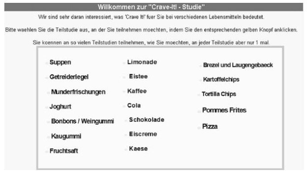
The respondent was invited by a local field service. There were 30 studies available for the respondent, who could only choose one. As soon as 130 respondents selected a study, and completed that study, the study temporary ‘disappeared’ from the of available studies from which one could choose. Figure 1 thus shows the 19 available studies in Germany, 11 studies having been completed for Germany. The respondent was sent to the study chosen. The study had to be complete in order to count against the quote of 120 respondent [15].

FIG 1

Figure 1: The ‘wall’ of available studies for the German Eurocrave project

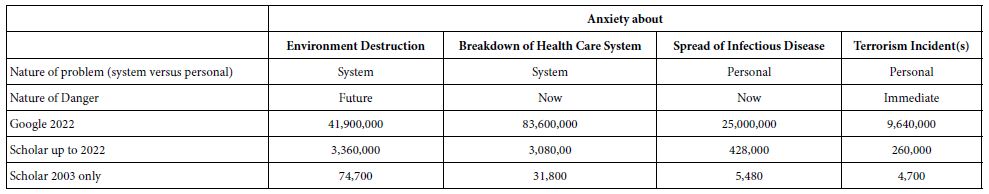
Moving to specifics, Table 1 shows the four questions for pizza, and the nine answers or elements for each question. Combinations of these text elements will become the stimuli that will be evaluated by the respondents. These combinations are known as vignettes. A hallmark of Mind Genomics is the effort made to have the elements present word pictures, not just simple phrases. That is, the elements or answers should paint an evocative picture involving pizza. The four questions provide a narrative of one’s experience with pizza.

Table 1: The 36 elements for pizza, shown in four groups. The respondent only saw the text, not the group, viz., not the organizing principle

table 1 (1)

table 1 (2)

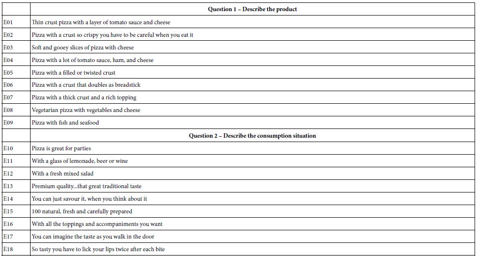
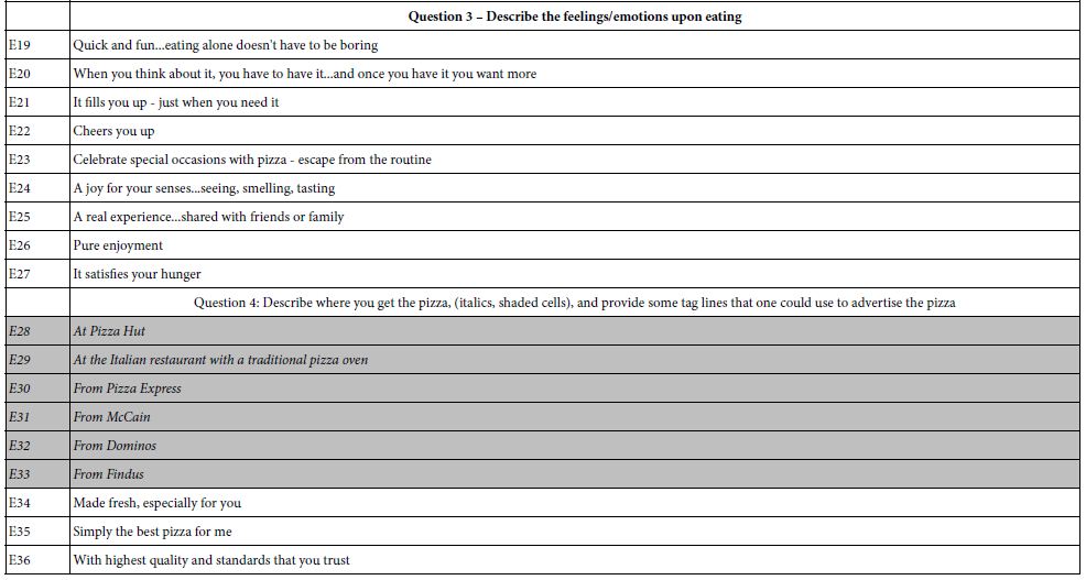
The Mind Genomics process executed in the early years of Mind Genomics (1996-2006), used a large experimental design, known as the 4 x 9, four questions or aspects, each with nine different elements. The 4 x 9 design involves 36 different elements, shown for pizza, in English. Table 1 shows these elements. As noted above, the elements present the outlets (Elements E28-E33) were particularized for each country, comprising the relevant outlets for those countries. The data from Question (E27-E36) will be used in the preliminary analysis in this study, but not discussed in the results, because of the difficulty of comparing across countries.

It is important to note that the Mind Genomics effort is not a single, final study which proposes to quantify the way people think about a product, in this case pizza. Rather, the Mind Genomics effort is simply an experiment, one experiment in a series when so desired, with the experiment showing concretely the importance of the element as a driver of attitude.

Once the elements have been chosen and polished, the next step is to combine these elements into small combinations, as noted above, the so-called vignettes. The rationale for vignettes are that we typically don’t see sequences of single ideas, one after another, to which we must react. Rather, we see combinations of pieces of information, often combinations which appear to be haphazard, or at least we fail in the short time allotted to uncover the pattern below the combinations. Yet, again and again we emerge unscathed from what seems to be hard to discuss, namely haphazard combinations. We react, and often don’t even realized the nature of our thinking.

The Mind Genomics was designed eliminate two biases. The first bias is that one-at-a-time presentation of messages is simply not the way we work. We are gluttons for information, of all types, mixed in ways.

The second bias is that we unconsciously adjust our thinking to accommodate the nature of the stimulus. We do not judge all stimuli the same way. For example, brand names are judged differently than product performance. The criteria we used to judge brand names versus product performance are different. The rationale, perceptive individual will adjust her or his criteria depending upon what particularly is being evaluated. For example, were we to read only the individual elements in Table 1, rating one element at a time, it might be easy to adopt different criteria, depending upon the specific element. If the respondent were answer elements from the set of E1-E9, the respondent might adopt the criterion of ‘do i like the flavor’. In contrast when it comes to the third set of elements (E19-E27), the criterion would not be ‘liking’, but rather fun to eat in a situation. The change in criterion might be quick, virtually unconscious, but sufficient to create a situation where the assessments might not be commensurate because the respondent uses different criteria, such criteria a function of the specific nature of the single message presented. What we measure, as a result, may seem like it should be valid because the respondent does the operation, but the validity might be a chimera, a false result.

Each respondent in the study is exposed to these elements, but in the form of vignettes. The vignettes are combinations of elements, as specified by an underlying experimental design. The design specifies combinations of 2-4 elements. Each vignette, the aforementioned combination, comprises at most one element from each group, but often the vignette is lacking one or two elements.

The specific structure of the vignettes, defined as the underlying experimental design, comes to 60 different combinations. Each respondent tests a different permutation of the basic design. That is, the mathematical structure of the 60 vignettes remains the same, but what changes is the specific set of 60 combinations. This strategy, working with a fixed design that is permuted, ends up having three key benefits:

1. Ability to Work with the Rating Scale, to Simplify it for the Manager

As noted above, the ratings, assigned on a 9-point scale (1=do not crave at all…. 9=crave extremely) are converted to a simpler binary scale (ratings 1=6 converted to 0, ratings 7-9 converted to 100). It will be these binary transformed ratings that will be used as the dependent variables in the individual-level and group models. After the transformation, a vanishingly small random number added to each transformed value (value < 10-5), in order to ensure that the binary transformed rating always shows some variation across the 60 vignettes evaluated by a single respondent.

2. Create a Model (viz., Equation) for Each Individual Showing How the Elements ‘Drive’ the Rating

Each respondent tests just the correct combinations to allow statisticians to estimate the contribution of each of the 36 elements to the rating. This is called a permuted design [12]. The ability to do the statistical modeling down to the level of a single respondent is very important. One does not need to balance the sample, and go through other ‘gyrations’ to ensure that the study is balanced The typical equation is expressed as: The typical equation is written as: (Binary Transformed) Rating = k0 + k1 (E01) + k2 (E02)…kn(E36).

3. No Requirement that the Researcher ‘Know’ the Correct Region to Test

The typical experiment covers so little ground that the typical experiments ends up validating the ingoing hypothesis of the researcher, rather than exploring and learning. In effect, the research focuses on a microscopically small volume of the possible design space. In contrast, with Mind Genomics, each respondent provides unique data, not provided by the other respondents. Each respondent provides a separately oriented snapshot of the mind of the respondent. The result is coverage of a lot of the possible combinations, albeit a coverage achieved with the aid of the many respondents. A good metaphor for the approach is the MRI used in medicine, which takes snapshots of the same tissue from different angles, and then reconstitutes a single snapshot of the tissue through computer analysis.

Coefficients for Product Elements (Total vs. Countries vs. Mind-sets)

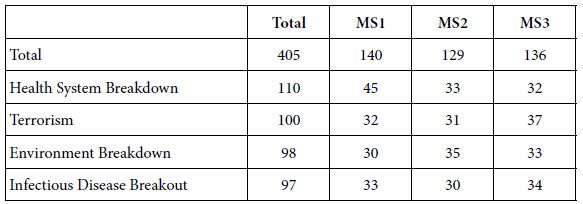
Our first focus will be on the coefficients achieved by E01-E09, the nine elements presenting information about the actual product itself, viz., the ingredients and the form. To summarize the analytic strategy, All data presented in Table 2 come from abstracting the coefficients for the individual models, these models having been created from the data for one respondent across the 60 vignettes, the 36 elements, and the rating scale transformed to a binary scale (0/100; ratings of 1-6 → 0; ratings 7-9 → 100).

Table 2: The coefficients for the nine description-based elements for pizza (E01-E09), and the additive constant. The numbers in the body of the table are the coefficients from the OLS (ordinary least-squares) models or equations relating the presence/absence of the elements to the transformed overall rating. The table only shows element coefficients of +10 or higher.

table 2 (1)

table 2 (2)

table 2 (3)

table 2 (4)

table 2 (5)

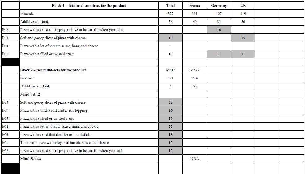
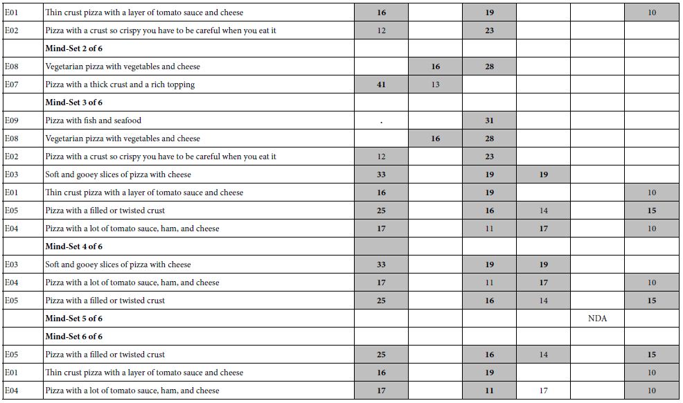
Mind Genomics studies ‘throw off’ a great deal of data. For most studies, it has become increasingly clear that the best way to discern patterns is to estimate all the coefficients, but then only focus on the coefficients which are strong. The large positive coefficients are the key elements which ‘drive’ the response. The small positive and many negative coefficients are harder to interpret, often adding noisy to what would otherwise be an easy naming.

Table 2 shows the coefficients for E01-E09, for six blocks of results. Recall that elements E01-E09 are features of the pizza. For the individual models, only coefficients of +10 or higher are shown. These coefficients are statistically significant, approaching a t-statistic of 2.0. The additive constant is shown for every key subgroup, however,

Block 1 = Total panel, France, Germany, United Kingdom

The data in Block 1 come from the coefficients for the total panel, without any further processing. The acceptance of pizza ranges from a low of 31 (Germany) to a high of 40 (France). What emerges is the modest acceptance of pizza without any elements, as shown by the modest-sized additive constant. It will be the elements which generate the acceptable.

It should not come as a surprise that when we deal with foods, the strong performing elements are those which present information about the product itself, the constituents, viz., and the ingredients. These elements are ‘concrete’, painting a word picture. For most food and beverage products, these are the elements which excite the consumer, even when the elements are embedded in a vignette with other information.

For the total panel, only two elements even reach the coefficient value 10: Soft and gooey slices of pizza with cheese and Pizza with a filled or twisted crust. It is important to keep in mind that these two elements deal with form, and do not invoke unusual flavors.

Blocks 2-6 (Clustering to Generate Mind-sets, viz., Segments of Respondents with Similar Patterns of Coefficients for Elements E01-E09

The initial analysis to generate the coefficients was done on the complete data-set for each respondent, viz., all 60 vignettes for the data base, and all 36 elements as independent variables. Thus each respondent generated a totally separate model, made possible by the previously discussed individual-level design. For the analyses in Blocks 2-6 m only the coefficients for E01-E09 were used in order to create the clusters, viz., and the mind-set. The method used was k-means clustering [16], with the measure of distance between pairs of respondents computed on the basis of the expression (Distance = 1-Pearson Correlation). It is important to emphasize that the clustering is done without any preconceived bias. The clustering algorithm is strictly an algorithm with no need to know the ‘meaning’ of the variables that it is using in its mathematical computations.

Block 2 (Two Mind-sets)

The simplest clustering using k-means clustering, ended up dividing the respondents into two groups, the basic likers (Mind-Set 22), and the feature likers (Mind-Set 21). Mind-Set 22 is larger, likes but does not love pizza (additive constant 55), and is indifferent to the features of the pizza. That is, no element emerge with coefficients over +10. In contrast, the smaller group Mind-Set 21), constituting approximately 1/3 of the respondents, shows a no general desire for pizza in the absence of elements (additive constant 5), but with a strong desire for the features of traditional pizza, Four examples of the exaggerated response by Mind-Set 21 to features (coefficient > 20) are:,

Soft and gooey slices of pizza with cheese

Pizza with a thick crust and a rich topping

Pizza with a filled or twisted crust

Pizza with a lot of tomato sauce, ham, and cheese

Block 3 (Three Mind-sets)

Mind-Set 32 is interested in pizza in general (additive constant 62), but does not find any of the product features very interest. In contrast, Mind-Sets 31 and 33 show low basic interest in pizza (additive constant 9 and 5), but strong interest in specific features of the product. Mind-Set 31 appears to want the more traditional features of pizza, whereas Mind-Set 33 appears to want to more ‘unusual features.’ It is important to keep in mind that these differences are not imposed on the data, but emerge from the patterns across people and countries.

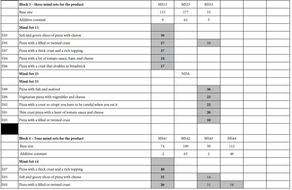
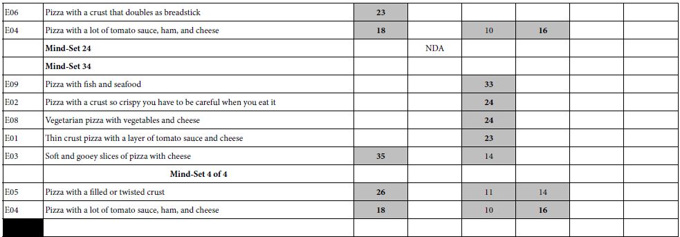
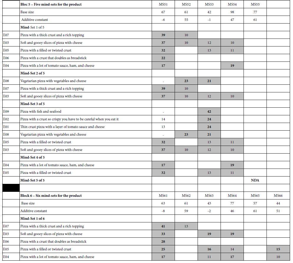
Block 4 (Four Mind-sets), Block 5 (Five Mind-sets), and Block 6 (Six Mind-sets)

These three additional clusters, again based only on the coefficients for E01-E9, show similar patterns.

a. One of the mind-set clusters shows a high additive constant, meaning that the respondents like all of the pizza ideas. This cluster, however, shows no elements describing the pizza which score very well. This cluster with the high additive constant is the non-discriminating, acceptor, abbreviated NDA.

b. The remaining mind-sets show different, unpredictable patterns, with low additive constant, but with some specific product elements presenting a very high coefficient.

c. An element can perform poorly with total panel, and with two or three mind-sets, viz., demonstrate a low positive coefficient, or a negative coefficient, but with more mind-sets extracted this poorly performing element, one that might be overlooked, might suddenly become promising. An example is: Pizza with fish and seafood.

d. Table 2 suggests that the dynamics of the system are complicated. An element may be irrelevant until a sufficient number of mind-sets or clusters are allowed, at which point the element shows its strength, and for one mind-set the element generates a high coefficient, whereas for the other mind-sets this previously ‘minor’ element remains minor.

e. The key word here is unpredictability. The lesson is the possibility of identifying mind-sets, albeit as an exercise in data analysis, and the practical use of the clusters for formulating marketing strategy. What is disappointing is the lack of specific, repeated patterns emerging from the clustering, patterns that could for the basis of a culinary psychology of pizza.

The Deeper Dynamics of Elements as Drivers of Mind-sets

It may well be that a different way is needed to understand the way elements perform. Rather than looking at the coefficient of the element in different arrays of mind-sets (viz., 2 vs. 3 vs. 4 vs. 5 vs. 6), an alternative way looks at the variability generated by the element vs. error, and seeing how much real variability the generates with increasing number of mind-sets. This second way computes the F ratio for each element, with the F ratio being a measure of signal to noise. Higher F ratios mean that the element really ‘drives’ the segmentation. Lower F ratios mean that the element does not ‘drive’ the segmentation.

For this analysis, we look at the three sets of elements (Question A – product features; Question B – Consumption Occasions; Question C – Emotional benefits and outcomes.). We do not look at Question D because the elements for the ‘purchase location’ (E28 – E33) changed by country.

The analyses are done separately question, following the approach below. We describe the approach for one of the three sets of elements. The same approach is applied separately to the other two sets of elements.

  1. For each question, collect all the sets of nine coefficients across all the respondents. Each respondent generates a row of nine numbers, one cell for each element. This step generated three data sets, based on elements E01-E09; E10-E18, and E19-E27, respectively,
  2. For each question separately, cluster the respondents, using the appropriate set of elements and their coefficients., Use k-means clustering as one before, with the distance between pairs of respondents defined as (1-Pearson R computed on the nine corresponding elements for the two respondents). Do the clustering five times, extracting first two clusters, then separately three clusters, then separately four clusters, then separately five clusters, and finally separately six clusters. The term ‘separately’ is repeated to emphasize the fact that the clustering starts anew each time.
  3. Estimate the F ratio for each of the nine elements. The magnitude of the F ratios is a measure of the degree to which the element ‘drives the segmentation.
  4. Keep in mind that the data set is balanced in terms of respondents. Thus, we have removed the subject effect, and dealing only with the degree to which the element drives the segmentation.

When we follow this protocol, computing the F ratio for each element when the clustering goes sequentially from two to six mind-sets, we uncover the deeper structure, viz. a structure which may truly underlie the different groups. Table 3 shows the F ratios for each of the 27 elements, computed for the five sequential clustering. Each clustering generates a set of 27 F ratios.

Table 3: F ratios for elements emerging from the clustering. High F ratios mean that the element is a strong driver of the classification. All F ratios of 10 or higher are shown in in a shaded ell

table 3

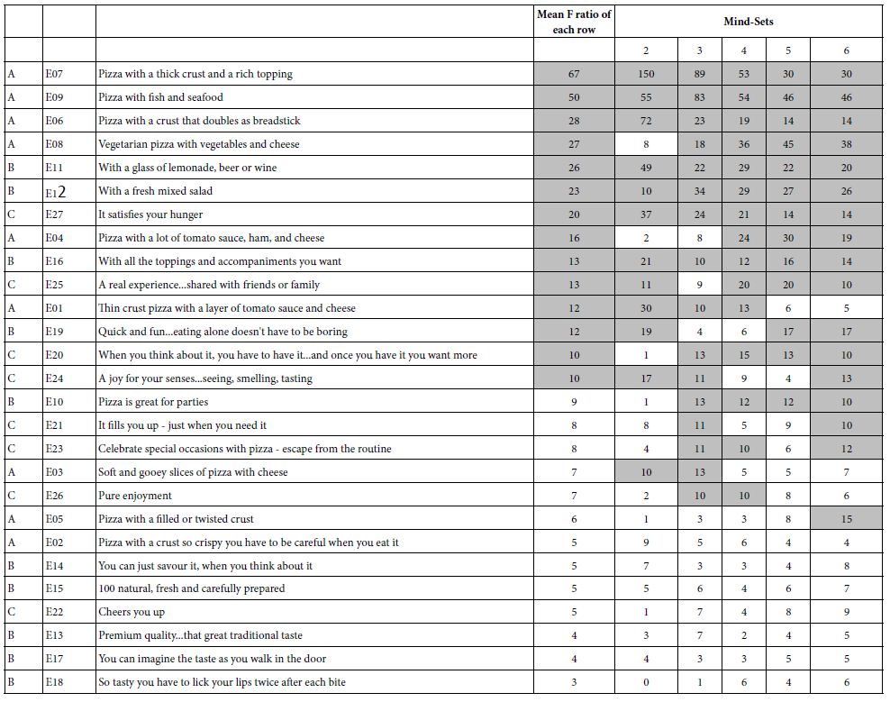
Keeping in mind that the F ratio is a measure of signal to noise, we can sort Table 3 five times, each time identifying the two (or more) strongest performers. The structure below begins to emerge, suggesting that there are two strong groups; traditional pizza and pizza with fish and seafood. There may be more, but these are the repeating themes.

Two mind-sets

Pizza with a thick crust and a rich topping

Pizza with a crust that doubles as breadstick

Three mind-sets

Pizza with a thick crust and a rich topping

Pizza with fish and seafood

Four mind-sets

Pizza with fish and seafood

Pizza with a thick crust and a rich topping

Five mind-sets

Pizza with fish and seafood

Vegetarian pizza with vegetables and cheese

Six mind-sets

Pizza with fish and seafood

Vegetarian pizza with vegetables and cheese

The dynamics of segmentation suggest that it is both the nature of the topic whose representatives are being segmented and the number of available segments which make a difference. An element may be less important than another when there are two or three segments, and so the less important element simply ‘goes along’. When it comes to more segment, e.g. four or five or six, this hitherto minor, unimportant element becomes important, and becomes the center of a new mindset. This finding may seem a bit awkward, but it is testimony to the fact that it is not only people differences in which are working, but the channels in which those differences are allowed to emerge. Reduce the opportunity and the segmentation waiting to flower is simply suppressed, not allowed to show itself.

The variability in preferences underlying the segmentation is clear greater for product (Question A), and then for emotion/benefit (Question C), and finally for consumption situation (Question B). One possible conclusion is that the potential segmentation is greatest for the actual product, something which manifests itself in the market today, where companies offering pizza offer different variations of them. The other groups offer the possibility of segmentation, but the F ratios are smaller. There are differences across mind-sets for a specific element, but there are few surprising re-emergences of elements as driers of segmentation when new mind-sets are opened up. The practical implication is that for marketing, most of the efforts, where possible, will be attempts to present new features of the pizza product itself.

Discussion and Conclusion

The world of foodservice is forever seeking to discover both what people like, and what they will like. There is the notion of habituation, that a stimulus which is presented again and again will lose its ability to excite [17,18]. People get bored with the same food, although the dynamics of such boredom, and habituation are yet to be worked out. One can see food trends come and go, with trend spotters looking for the latest and greatest, the cuisines, and of course the star items that will excite everyone. At the same time, observations in restaurants, especially diners with their massive choice of foods, suggest that people often stick with the same foods, no matter how big the choice. Indeed, the notion of paradox of choice has been raised to describe the observation that the larger the choice, the more conservative people become, often reverting to their favorite [19].

When we narrow our focus from the world of foods to the world of pizza we turn from a world of products people may or may not like to a world of product variations of what we might be to be a basically acceptable product. Indeed, for the most part people assume that pizza is a universally loved product, perhaps one of the most beloved in the world.

The data from this study suggest that the world of pizza comprises a universe until itself. The data suggest that there is strong differentiation among the different aspects of pizza, the strong differentiation appearing in issues involving the ingredients and flavors, less so in issues involving emotion and consumption situation.

The Pizza Study in the Context of Mind Genomics and the It! Studies

When the study was run two decades, in 2002, the ingoing assumption was that we would naturally uncover country to country differences in what people liked in pizza, especially the flavors of the pizza. It was intuitively obvious that we would not find a simple linkage between country and preference for pizza flavor. That would be too easy, too deceptive, even though one of thinks of countries in terms of ‘general preferences’, based upon the cuisines they offer. With pizza, the ingoing assumption was that we would find groups of respondents with clearly different mind-sets, different tastes as reflected in their responses to the different elements describing pizza [20], and then use these patterns of preferences to create new foods.

The structure of the worked-up data, after an interval of two decades, presents a working model of how thinking underlying Mind Genomics has evolved. The original efforts in Mind Genomics, represented most faithfully in the parallel studies known as the It! research, appeared to stop at the remarkable discovery that across products and countries, three different ‘canonical’ mind-sets would emerge, especially for foods and beverages. These mind-sets were the Traditionalists who wanted things the way they had always been; the Experientials ls who responded strongly to the description of emotions and situations; and finally the Elaborates who respondent most strongly the fancified description of the product features [13]. At the time of the initial analyses, the recurring pattern across foods sufficed excite. The patterns seemed repetitive, and worthy of report.

Over the years, however, as the data from the It! studies led to practical applications, the applications themselves opened up new issues, such as discovering relevant but numerically small groups of what would be important respondent groups. The solutions, clustering the data to smaller and smaller groups, began to provide business answers, such as the discovery of key groups. At the same, the dynamics suggested that such groups might be found in flavor, but not necessarily in packaging, and so forth. It was the demand for understanding the data in a deeper fashion which has led to the reanalysis of data, a reanalysis eminently possible because of the tight, comprehensive, balanced structure of the underlying permuted experimental design. This paper may be seen as a continuation of the early effort, using the same data, but with the experience and insight of two decades, along with the realization that these It! studies were stepping forth onto a new continent, with new horizons. This paper is a progress report, appearing two decades later.

Acknowledgment

The author acknowledges the efforts and inputs of his colleagues of two decades ago, Pieter Aarts of Belgium, and Klaus Paulus of Germany and the contribution of the late Hollis Ashman of the Understanding and Insight Group. The studies reported here were done under the aegis of It! Ventures, Inc., and are published with permission of It! Ventures, Inc.

References

  1. Luce RD, Krumhansl CL (1988) Measurement, scaling, and psychophysics. Stevens’ handbook of experimental psychology 1: 3-74.
  2. Peter JP, Olson JC, Grunert KG (1999) Consumer behaviour and marketing strategy (pp. 329-348). London, UK, McGraw-hill.
  3. Mead R (1990) The design of Experiments: Statistical Principles for Practical Applications. Cambridge University Press.
  4. Rokach L, Maimon O (2005) Clustering methods. In Data Mining and Knowledge Discovery Handbook (pp. 321-352). Springer, Boston, MA.
  5. Moskowitz HR, Papajorgji P, Wren J (2020) Mind Genomics and the Law, Chapter 5, Arson & Murder. Lambert Publications, Germany.
  6. Rubin H, Craig Wallace, Darry Rawlings (Trupanion senior management) Personal communication to Howard Moskowitz and Stephen Onufrey, June 2010).
  7. Moskowitz HR (2014) Mind Genomics and Texture: The experimental science of everyday life. In: Food Texture design and optimization (ed.Dar, Y.L. and Light, J.M) Helstosky C (2008) Pizza: a global history. Reaktion books.
  8. Jaitly M (2004) Symposium 4: Food Flavors: Ethnic and International Taste Preferences: Current Trends in the Foodservice Sector in the Indian Subcontinent. Journal of Food science 69: SNQ191-SNQ192.
  9. Kumar R (2015) A comparative study between Pizza Hut and Domino’s Pizza. International Journal of Marketing and Technology 5: 89-123.
  10. Lestari AD, Baktiono A, Wulandari A (2020) The effect of market segmentation strategy on purchasing decisions of pizza in Surabaya. Quantitative Economics and Management Studies 1: 1-8.
  11. Gofman A, Moskowitz H (2010) Isomorphic permuted experimental designs and their application in conjoint analysis. Journal of sensory studies 25: 127-145.
  12. Moskowitz MR., Ashman H, Minkus-McKenna D, Rabino S, Beckley JH (2006) Data basing the shopper’s mind: approaches to a ‘Mind Genomics’. Journal of Database Marketing & Customer Strategy Management 13: 144-155.
  13. Moskowitz HR, Gofman A (2007) Selling Blue Elephants: How to Make Great Products that People Want before They Even Know They Want them. Pearson Education.
  14. Aarts P, Paulus K, Beckley J, Moskowitz HR (2002) September. Food craveability and business implications: The 2002 EuroCrave™ database. In ESOMAR Congress, Barcelona, Spain.
  15. Likas A, Vlassis N, Verbeek JJ 2(003) The global k-means clustering algorithm. Pattern Recognition 36: 451-461.
  16. Fishbach A, Ratner RK, & Zhang Y (2011) Inherently loyal or easily bored?: Nonconscious activation of consistency versus variety seeking behavior. Journal of Consumer Psychology 21: 38-48.
  17. Zeithammer R, Thomadsen R (2013) Vertical differentiation with variety-seeking consumers. Management Science 59: 390-401.
  18. Schwartz B (2004) January. The Paradox of Choice: Why More is Less. New York: Ecco.
  19. Gere A, Moskowitz H (2021) Assigning people to empirically uncovered mind-sets: a new horizon to understand the minds and behaviors of people. Consumer‑based new product development for the food industry. Royal Society of Chemistry 132-149.

Commentaries on the Nature of Virus Species and Viral Vaccines and on Anglicized and New Latinized Species Names Used in Viral Taxonomy

DOI: 10.31038/JCRM.2022533

Abstract

Although one often talks of immunogenic viruses as being capable of generating protective antibodies against viral infections, it is actually the immune system of vaccinees that triggers in the host a series of reactions with B cell and T cell receptors that eventually leads to immune protection.

The chemical nature of antigenicity is often confounded with the biological nature of immunogenity and instead of designing a vaccine immunogen capable of generating protective Abs, investigators are sometimes only improving the binding reactivity (i.e. antigenicity) of a single viral epitope.

It is now well-established that the X-ray crystallographic structures of bound epitopes-paratopes visualized in an antigen-Ab complex are usually very different from the structures in the free binding sites before they had been altered by the mutual adaptation and induced fit that always occurs when the two partners interact. This means that the structure of the epitope that is required for inducing neutralizing antibodies by vaccination must be that of the free unbound epitope site, although investigators often opt for using an engineered bound epitope structure for vaccination purposes.

Keywords

ICTV proposals, Immune systems but not viruses elicit protective antibodies, Definition of virus species, Anglicized non-latinized virus names, Latinized binomial names

The Nature of Virus Species

Viruses are chemical objects which parasitize the genomes of animals, plants and microbial organisms that they have infected, and it is these living infected host cells that reproduce the viruses since viruses themselves are not alive [17-23]. Viruses are classified by using the hierarchical conceptual taxa known as species, genera, families and orders created by taxonomists which are used in all biological classifications [4,17,23,33]. The members of the lowest virus species class are also members of the classes above it and the relation between a lower taxon and higher ones is called class inclusion. Class inclusion avoids the need to repeat the properties used for defining higher taxa in the definition of the lower taxa that are included in them. Because of class inclusion, higher taxa such as genera and families always have more members than species which means that they require fewer properties (for instance the type of genome replication) to meet the qualification for membership. The logical principle which requires that it is necessary to increase the number of qualifications for defining a species actually invalidates the widespread belief among virologists that it is possible to define a species by the presence of a single short nucleotide in the viral genome [1,11,28], Since a virus species always has fewer members than genera and families, it is actually imperative to use several different properties for demarcating a new species [36]. Since the concept of a polythetic species cannot be described, it can only be defined by listing the number of the species-defining properties of its members which are not all necessarily present is every member of a polythetic species. Only monothetic species are defined by a few properties that are both necessary and sufficient for membership in the class, whereas the members of a polythetic class do not have a common property present in all its members. The term polythetic refers to a particular distribution of properties in the class and the members of the class do not themselves possess polythetic properties [3,15]. Gibbs & Gibbs et al 2006 argued that the term polythetic should be removed from the species definition because they viewed a virus species as a monothetic class whose members necessarily share a common property inherited from its ancestors and they removed the term polythetic from the definition of a virus species [11]. The species concept has remained controversial in biology [22] and in 1989 the following definition of virus species was proposed: “A virus species is a polythetic class of viruses that constitute a replication lineage and occupy a particular ecological niche [31]. This definition was approved by the International Committee on Taxonomy of Viruses (ICTV) [26].

The ICTV is a committee created in 1966 by the Virology Division of the International Union of Microbiologial Societies which is responsible for the development of a viral taxonomy and nomenclature and it has so far published ten Reports describing thousands of viral taxa [2,7,8,10,16,20,21,24,32,42]. The first Reports advocated a Latinized viral nomenclature for virus species which was abolished after a few years and was replaced by Anglicized species names.

It is important to differentiate between properties useful for defining a virus species and properties used for identifying individual viruses. Species taxa are defined intentionally by what is called the intention of the class which refers to the properties that provide the qualification for membership in the species. The so-called extension of the species class refers to the set of all the concrete members of the class. Since the intention of a class determines its extension, the extension of a class can only be determined if it is possible to distinguish members from non-members, which means that the intention must precede the extension [18]. A species taxon must therefore be established by taxonomists before it become possible to ascertain if a sufficient number of species-defining properties are present in an individual virus to make it a member of the species. Since monothetic species classes are defined by one of very few properties that are both necessary and sufficient for membership in the class, the claim of Gibbs& Gibbs (2006) that it is possible to rely on the presence of a single nucleotide motif for demarcating a new monothetic species is not realistic because it would be necessary to know beforehand that this motif is present in all the members of the species and absent in other species; this means that the extension would need to precede the intension which is of course impossible [11].

Bionominalism in taxonomy views species as individual and historical entities [15] that form cohesive wholes and accepts that a species lineage is a concrete object although it is a case of logical reification (i.e. viewing an abstract concept as if it were an object). The relational concepts of ancestry and lineage are actually not real objects and they cannot act upon each other unless they exist at the same time [18] Species also cannot descent from each other in a literal sense since only concrete organisms and viruses can do this. A species must therefore first be established and defined by taxonomists before it becomes possible to allocate a virus to a species by using so-called diagnostic properties. Such specific tools can be obtained by developing polyclonal or monoclonal antibodies against viruses that are members of the species although such antibodies are not species-defining properties that could have been used for demarcating the species taxon initially.

The term species in virology is used to refer 1) to the many individual species classes created by virologists that have viruses as their members and 2) to the lowest “category” in a virus classification which is the class of all the species that virologists have demarcated. The 1989 polythetic species definition actually refers to the species category which is of little help to virologists when they attempt to allocate viruses to a new species taxon.

The members of a polythetic virus species always share several relational phenotypic properties that arise by virtue of relations between the virus and its hosts and vectors which become actualized only during the transmission and infectious processes. These species-defining properties are easily altered by a few mutations which could modify the host range, the pathogenicity and cell and tissue tropism, and taxonomists often have to create species by drawing boundaries across a continuum of phenotypic and genetic variability.

Anglicized Non-Latinized Virus Species Names and Latinized Linnaean Binomial Names

Anglicized non-Latinized binomial names (NLBNs) for species were initially introduced by Fenner [8] by replacing the terminal word virus that occurs in all English virus names with the name of the genus to which the virus belongs and will also ends in virus. Measles virus for instance became a member of the italicized species Measles morbillivirus and thousands of such names became very popular since genus names and English names of viruses are well known to all virologists. This is due to the fact that the major reference books in virology as well as the numerous ICTV Reports published during the last 45 years were written in English which is the predominant communication language used by scientists. In 2016, the ICTV initiated a so-called thought exercise in which they converted currently existing 175 NLBNs into an inverse Latinized Linnaean binomial format (LLBNs) that consists of the genus name followed by a Latinized epithet [25]. Adelaide River virus for instance became the NLBN Adelaide River Ephemerovirus while the LLBN was Ephemerovirus fiumeadelaidense. NLBNs are easily recognized by virologists and quarantine officials whereas the epithets may be less obvious. The ICTV nevertheless approved the introduction of LLBNs [42] and the ICTV Study Groups were given the task of converting thousands of NLBNs into the new LLBN format which is expected to be completed in 2013. No explanation was presented for removing thousands of popular Anglicized NLBNs for non-living virus species and for following the Linnaean format used for living organisms. Virus species were redefined as groups of living physical isolates which is not in line with the definition of all the biological species of organisms as being abstract conceptual classes [42].

Adrian Gibbs has for years been a regular critic of ICTV proposals and decisions [11-13] and in a recent review [14] he analyzed two proposals that the ICTV had presented as a consensus statement [29] and a consultation [27]. With the rapid development of high-throughput sequencing methods for viral genomes, large numbers of virus-like gene sequences called metagenomes had been obtained from a variety of living materials.

The ICTV Executive Committee reacted to this avalanche of sequences by organizing a workshop attended by viral taxonomists who produced a so-called consensus statement that accepted that these virus-like metagenomes corresponded to viral genomes that should be incorporated in the existing ICTV taxonomy, in spite of the absence of any known biological properties of what were nevertheless referred to as sequence-viruses [47]. Since the hosts and vectors linked to most of these sequences had not been identified these sequence-viruses were indeed only sequences. Gibbs [14] reminded virologists that the ICTV taxonomy should be a taxonomy of viruses but not of virions nor of gene sequences. Gibbs endorsed the view that viruses are subcellular organisms with a two-part so-called life cycle, namely virions and virus-infected host cells which is a terminology proposed earlier by Forterre [9], in spite of the fact the majority of virologists still consider viruses to be non-living genetic parasites [17] devoid of any metabolic activity [36]. Many virologists remain convinced that species and other taxonomic classes in virology and biology are not abstract constructs of the human mind and they do not accept that conceptual taxonomic classes can have tangible, material objects and organism as their members. In 2013 the ICTV has ratified the following species definition: A species is a monophyletic group of viruses whose properties can be distinguished from those of other species by multiple criteria [1]. This definition which is applicable to any taxonomic class is incompatible with the logic of classes based on class inclusion used in all biological classifications and this has given rise to numerous debates [16,36].

The Immune System of Vaccinees rather than Immunogenic HIV Viruses are Able to Elicit Anti-viral Protective Antibodies against AIDS

Although one often talks of immunogenic viruses as being capable of generating protective antibodies against viral infections, Although It is actually nearly always the immune system of vaccinees that triggers in the host a series of reactions with B cell and T cell receptors which eventually leads to immune protection [30], many vaccinologists have for many years elucidated the structure of the antigenic epitopes in virions because they assumed that these epitopes when used as immunogens would be able to induce protective antibodies against viral infection. They used an approach [5] called structure-based reverse vaccinology (SBRV) to determine the structure of complexes between viral epitopes and neutralizing Monoclonal Antibodies (nMAbs) obtained from patients infected for instance with HIV, in an attempt to design HIV immunogens by reverse molecular engineeing that would elicit neutralizing antibodies (nAbs) [39].This approach was called reverse vaccinology because investigators assumed that if an antigenic epitope did bind strongly to an nMA, it would also be able to induce similar nAbs when used as a vaccine [34]. They also assumed that when an epitope binds to a free antibody molecule, the recognition process is exactly the same as when that epitope (which is now called an immunogen) binds to a cognate B cell epitope receptor embedded in a lipid membrane.

An additional problem with the SBRV approach was that it ignored the fact that all Abs are always polyspecific or even heterospecific [35] and that antigenic and immunogenic regions in a protein antigen are often located in different parts of the molecule [39].

Many constituents of immune systems are known to control the types of Abs that are produced, such as the host Ab gene repertoire, as well as other regulatory mechanisms, although investigators may only pay attention to individual recognition processes between single epitope and paratope pairs. When it was found that HIV Env epitopes recognized by affinity-matured Abs obtained from HIV-infected individuals did not bind the germline predecessors of these Abs [30,44] it became obvious that potential vaccine immunogens would only be discovered if one took into account the extensive Ab affinity maturation that is required for obtaining Abs that neutralize HIV. A huge research effort was then initiated to analyze the innumerable maturation pathways that can lead to protective Abs [19].

The chemical nature of antigenicity is often confounded with the biological nature of immunogenity and instead of designing vaccine immunogens capable of generating protective Abs, investigators may only attempt to improve the binding reactivity (i.e.antigenicity) of a single viral epitope.

Epitopes in antigens and paratopes in immunoglobulins are rather flexible and dynamic binding sites and their plasticity has been compared to flexible keys and adjustable locks [6]. It is now well-established that the X-ray crystallographic structures of bound epitopes and paratopes visualized in an antigen-Ab complex that are mostly very different from the structures in the free binding sites before they have been altered by the mutual adaptation and induced fit that always occurs when the two partners interact [43]. The epitope structure observed in the epitope-paratope complex is therefore a poor experimental model for trying to elicit again the type of Ab that was used in the crystallograhic binding experiment. It is in fact even difficult to comprehend why adepts of SBRV continued for many years to try to develop HIV vaccines using that approach, since the crystallographic structure of the bound model epitope clearly showed that it was unlikely to be able to elicit the type of protective Abs that is aimed for [35-37,40].

References

  1. Adams MJ, Lefkowitz EJ, King AMQ, Carstens EB (2013) Recently agreed changes to the international code of virus classification and nomenclature. Arch Virol 158: 2633e9. [crossref]
  2. Adams MJ, Lefkowitz EJ, King AMQ, et al. (2017) 50 years of the International Committee on Taxonomy of Viruses: progress and prospects. Arch Virol 162: 1441-1446. [crossref]
  3. Beckner M (1959) The biological way of thought. New York: Columbia University Press.
  4. Buck R, Hull D (1966) The Logical Structure of the Linnaean Hierarchy. Systematic Zoology 15: 97.
  5. Burton D (2002) Antibodies, viruses and vaccines. Nature Reviews Immunology 2: 706-713. [crossref]
  6. Edmundson A, Ely K, Herron J, Cheson B (1987) The binding of opioid peptides to the Mcg light chain dimer: Flexible keys and adjustable locks. Molecular Immunology 24: 915-935.
  7. Fauquet C, et al. (2005) Virus Taxonomy. Eighth Report of the ICTV. Elsevier, Academic Press. London, San Diego.
  8. Fenner F (1976) Classification and Nomenclature of Viruses. Second Report of the ICTV. Intervirology 7: 1-115.
  9. Forterre P (2103) The virocell concept and environmental microbiology. ISME J 7: 233-236. [crossref]
  10. Francki RIB, et al. (1991) Classification and Nomenclature of Viruses Fifth Report of the ICTV. Arch Virol 2.
  11. Gibbs A, Gibbs M (2006) A broader definition of ‘the virus species’. Archives of Virology 151: 1419-1422. [crossref]
  12. Gibbs AJ (2003) Virus nomenclature: where next. Arch Virol 148: 1645e53.
  13. Gibbs AJ (2013) Viral taxonomy needs a spring clean; its exploration era is over 10: 254.
  14. Gibbs AJ (2020) Binomial nomenclature for virus species: a long view. Arch Virol 165: 3079-3083. [crossref]
  15. Hull DL (1976) Are species really individuals? Syst Zool 25: 174e91.25
  16. King AMK, et al. (2012) Virus Taxonomy. Ninth Report of the ICTV. Elsevier, Academic Press, London, San Diego.
  17. Lwoff A (1957) The Concept of Virus. Microbiology 17: 239-253.
  18. Mahner M, Bunge M (1997) Foundations of biophilosophy. Berlin: Springer-Verlag.
  19. Mascola J, Haynes B (2013) HIV-1 neutralizing antibodies: understanding nature’s pathways. Immunological Reviews 254: 225-244. [crossref]
  20. Matthews REF (1979) Classification and Nomenclature of Viruses. Third Report of the ICTV. Intervirology 12: 129-296.
  21. Matthews REF (1982) Classification and Nomenclature of Viruses. Fourth Report of the ICTV. Intervirology 17: 1-199.
  22. Mayden RL (1997) A hierarchy of species concepts: the denouement in the saga of the species problem. In: Claridge MF, Dawah HA, Wilson MR, editors. Species: The Units of Biodiversity. Chapman and Hall, London. 381-424.
  23. Moreira D, López-García P (2009) Ten reasons to exclude viruses from the tree of life. Nature Reviews Microbiology 7: 306-311. [crossref]
  24. Murphy FA, et al. (1995) Virus Taxonomy Sixth Report of the ICTV. Springer, Vienna, New York.
  25. Postler TS, Clawson AN, Amarasinghe GK, Basler CF, Bavari S, et al. (2017) Possibility and challenges of conversion of current virus species names to Linnaean binomials. Syst Biol 66: 463-473. [crossref]
  26. Pringle CR (1991) The 20th Meeting of the Executive Committee of the ICTV. Virus species. higher taxa and other matters. Arch Virol 119: 303-304.
  27. Siddell SG, Walker PJ, Lefkowitz EJ, Mushegian AR, Dutilh BE, et al. (2020) Correction to: Binomial nomenclature for virus species: a consultation. Arch Virol 165: 1263-1264. [crossref]
  28. Simmonds P (2015) Methods for virus classification and the challenge of incorporating metagenomic sequence data. Journal of General Virology 96: 1193-1206. [crossref]
  29. Simmonds P, Adams M, Benkő M, Breitbart M, Brister JR, et al. (2017) Virus taxonomy in the age of metagenomics. Nat Rev Microbiol 15: 161-168. [crossref]
  30. Van Regenmortel MHV (2013) An oral tolerogenic vaccine protects macaques from SIV infection without eliciting SIV-specific antibodies nor CTLs. J AIDS Clin Res 4: e112.
  31. Van Regenmortel MHV (1990) Virus species, a much overlooked but essential concept in virus classification. Intervirology 31: 241-254. [crossref]
  32. Van Regenmortel MHV, et al. (2000) Virus Taxonomy. Seventh Report of the ICTV. Academic Press, New York.
  33. Van Regenmortel M (2010) Logical puzzles and scientific controversies: The nature of species, viruses and living organisms. Systematic and Applied Microbiology 33: 1-6.
  34. Van Regenmortel MHV (2012b) Basic research in HIV vaccinology is hampered by reductionist thinking. Front Immunol 3: 194. [Crossref]
  35. Van Regenmortel M (2014) Specificity, polyspecificity, and heterospecificity of antibody-antigen recognition. Journal of Molecular Recognition 27: 627-639. [crossref]
  36. Van Regenmortel MHV (2016) Classes, taxa and categories in hierarchical virus classification: a review of current debates on definitions and names of virus species. Bionomina 458: 101-121.
  37. Van Regenmortel M (2016) Structure-Based Reverse Vaccinology Failed in the Case of HIV because it Disregarded Accepted Immunological Theory. International Journal of Molecular Sciences 17: 1591. [crossref]
  38. Van Regenmortel M (2016) Commentary: Basic Research in HIV Vaccinology Is Hampered by Reductionist Thinking. Frontiers in Immunology 7: 7875. [crossref]
  39. Van Regenmortel M (2019) HIV/AIDS: Immunochemistry, Reductionism and Vaccine Design, A Review of 20 Years of Research. Springer Verlag, Switzerland.
  40. Van Regenmortel M (2011) Two meanings of reverse vaccinology and the empirical nature of vaccine science. Vaccine 29: 7875. [crossref]
  41. Walker PJ, Siddell SG, Lefkowitz EJ, Mushegian AR, Adriaenssens EM, et al. (2021) Changes to virus taxonomy and to the International Code of Virus Classification and Nomenclature ratified by the International Committee on Taxonomy of Viruses. Arch Virol 166: 2633-2648. [crossref]
  42. Wildy P (1971) Classification and Nomenclature of Viruses. First Report of the ICTV. Monographs in Virology 5.
  43. Wilson I, Stanfield R (1994) Antibody-antigen interactions: new structures and new conformational changes. Current Opinion in Structural Biology 4: 857-867. [crossref]
  44. Xiao X, Chen W, Feng Y, Zhu Z, Prabakaran P, et al. (2009) Germline-like predecessors of broadly neutralizing antibodies lack measurable binding to HIV-1 envelope glycoproteins: Implications for evasion of immune responses and design of vaccine immunogens. Biochemical and Biophysical Research Communications 390: 404-409. [crossref]
  45. Van Regenmortel MHV (2017) Immune systems rather than antigenic epitopes elicit and produce protective antibodies against HIV. Vaccine 35: 1985-1986. [crossref]
  46. Hull DL, Rima B (2020) Virus Taxonomy and classification: naming of virus species Arch Virol 165: 2733-2736.
fig 1

Fearing Now, Fearing Later: A Mind Genomics Cartography

DOI: 10.31038/ASMHS.2022652

Abstract

A total of 405 respondents evaluated different vignettes (combinations of messages) in four separate but parallel studies, these studies dealing with the breakdown of the healthcare system, the breakdown of the environment, the spread of infectious disease, and terrorist incidents, respectively. The combinations of messages were created by experimental design, allowing statistical deconstruction of the messages into additive models, with each element generating a coefficient showing how the element drives the rating of ‘can’t deal with the situation’. Ten messages were the same across the studies, and were extracted for comparative analysis. Clustering the pattern of these ten coefficients across the four studies, independent of study, suggested three groups; Mind-Set 1: Low basic anxiety but sensitive to specific stressors”; Mind-Set2: “Not particularly discriminating but also possibly anti-religious”; Mind-Set 3:“Overwhelmed and obsessive”. The analysis provides a new approach to understanding how people respond to anxiety-provoking situations, an approach emerging from experimentation rather than from personality-oriented psychological research.

Introduction

As this century proceeds, we are increasingly accustomed to news which increases our anxiety. One need only listen for a half hour of news to hear of unexpected failures of the government to protect its citizens, the fear in the population caused by terrorists who deliberately destroy property and people alike, the rampant diseases which can shut down entire nations as did the Covid-19 virus, and of course those who proclaim that the environment is on its way to making the world inhabitable. One does not need a set of published references for these and many other causes of anxiety. The newspapers will do. But for those who are interested, a sense of the importance of the topics can be seen in Table 1. Table 1 shows the number of ‘hits’ from a search of the four topics, first using Google (up to and including 2022), then Google Scholar (up to and including 2022), and finally Google Scholar only for 2003, the year that the study was run. What is interesting is the focus on the heath system and the environment as most important. Both of these may be said to be future rather than immediate.

Table 1: ‘Hits’ produced by a Google® and Google Scholar® search

table 1

The four studies reported here come from an attempt undertaken almost two decades ago, in 2003, to understand the way people think about problem situations. The approach was rooted in background of consumer research, experimental psychology, and statistical design. Rather than asking people to talk about problems, something that is commonly done by qualitative researchers, the focus was to systematically create combinations of messages (vignettes), dealing with issues presumed to drive anxiety (e.g., issues about the destruction of the environment), present these vignettes to respondents, obtain a rating of the vignettes and then deconstruct the ratings into the part-worth contribution of each element as it drives the feeling of ‘can’t deal with it.’

The approach just described above is a process which began as a standard research approach called conjoint analysis [1], and evolved into a variation called Mind Genomics [2,3]. The difference is simple. Both methods, conjoint analysis and Mind Genomics, work with a set of basic ideas or messages, which messages are combined by an underlying procedure known as experimental design [4]. Conjoint Measurement creates one set of combinations, and presents this one set of combinations to many respondents, each respondent evaluating the same combinations but of course in a different order to reduce so-called order bias. One of the benefits of Conjoint Measurement was the fact that it required the researcher to think deeply about the topic, and to create the single set of vignettes, the combinations of messages, in such a way that they made sense.

Some years after the introduction of Conjoint Measurement in its mathematical psychology form, viz., theory, by mathematical psychologists [1] and the popularization by Wharton School professors Paul Green and Jerry Wind [5], it became obvious that one improvement might alleviate the problem of requiring the ‘right guess’ about the vignettes to test. This improvement was to create a basic experimental design, as does Conjoint Measurement, but then permute the design, so each respondent evaluates vignettes created according to the same design structure, but the actual combinations would change [6]. In simple terms, this meant that each respondent would evaluate what turns out to become a totally separate set of combinations.

The experimental design ensures that the elements or messages are statistically independent of each other, allowing for analysis by standard, off-the-shelf methods like OLS (ordinary least squares) regression. The analysis enables the researcher to estimate the contribution of each element in the vignette as a ‘driver’ of the response. Equally important was the realization that no one had to know ‘the answers’ ahead of time, nor spend time identifying the ‘best combinations’ to test. By having each respondent evaluate different permutation of the design, in effect the strategy makes conjoint measurement into an exploratory tool, not a confirmation of one’s best guess. One could go into the study without any knowledge, and still identify ‘what works’.

The foregoing leap, from one design to many designs, is reminiscent of the advances made by the MRI, which takes many ‘pictures’ of a single underlying object, such as body tissue, each picture from a different angle. Afterwards, the computer program recombines these pictures into a three-dimensional representation of the underlying object. In a like manner, the Mind Genomics approach takes many ‘pictures’ of the topic, each picture dictated by the specific combinations in a single permuted design. The result is that for say 100 respondents, one can create a much more detailed, more inclusive picture of the underlying topic, testing the response to many different combinations, rather than testing the response to one combination many times.

The It! Studies and specific ‘Deal With It!’

The development of Mind Genomics software during the late 1990’s and early 2000’s allowed the researcher to set up studies using the Mind Genomics platform. During that time, the author’s business (Moskowitz Jacobs, Inc.) expanded the use of Mind Genomics, moving to studies about the everyday. The ability to set up studies with as many as 36 messages (elements), run the studies using the permuted design, and return in a few hours with the results allowed Mind Genomics to deal with topics on a wider scale. By ‘wider scale’ is meant that that a research project would not be limited to one specific topic, such as the best messages for coffee but might comprise 15-30 related studies, e.g., on foods or beverages [7]. These studies would constitute ‘foundational studies’ of a topic, studies deal with the ordinary facets of daily life, and in their entirety constituting a new form of integrated database about human decision in the ‘everyday’ world.

The four studies reported here come from a of 15 studies called Deal With It!, studies dealing with anxiety-provoking topics. The specific focus in this paper is the response to a set of messages, each of which was the same but in four topics: Environment Degradation, Infectious Disease, Breakdown of the Health Care System and Terrorist acts, respectively. The objective was to understand the degree to which messages about these 15 different anxiety-provoking situations would be perceived as most disturbing. The studies comprise two involving the person in an intimate way (terrorism, spread of infectious disease, particularly relevant in an age of Covid-19), and two involving a breakdown in external structure, (breakdown of the health care system; breakdown of the environment).

The topics were selected from a variety of issues current in the early years of this millennium. The respondents were invited to participate, and selected the one topic which interested them. All 15 topics were available for choice. Figure 1 shows the ‘wall’ of studies available to the respondent. The respondents were invited by a Canadian company, Open Venue Ltd. Which provided respondents from the United States.

fig 1

Figure 1: The ‘wall’ of the 15 available studies for the ‘Deal With It! Project

Elements (Messages) The Raw Materials for the Study

A hallmark of the It! studies, such as Deal With It! comes from the fact that for the most part the elements or messages in the studies are either parallel or often the same. Table 2 shows the array of 36 elements used in the Terrorism study. The underlying structure of the study comprises four questions, these questions remaining the same across all 15 studies (e.g., Question 1, What Happens), etc.

Table 2: The 36 elements for the Deal With It! study on terrorism, showing the rationale for each element and the actual element

table 2

The left side of Table 1 shows the ‘rationale’ for the element. The right side of Table 1 shows the specific text for the answer. Each of the four questions generates nine answers, the elements. The actual questions and answers are left to the researcher, with the Mind Genomics process providing only the design and research template. Across all 15 studies, only Question 3 used the same elements. The three remaining questions comprised answers appropriate for the topic. The analysis in this paper will use only the nine elements or answers generated from Question 3 (elements E19-E27), and the God answer, E28. The texts of these elements were almost identical across the studies.

The Mind Genomics process works by combining elements (answers to questions), according to an underlying experimental design. The combination is put together so the elements appear stacked, one atop the other, without connectives, as shown in Figure 2. The actual experimental design comprises 60 vignettes or combinations with the number of elements in each vignette varying from as few as two to as many as four. The elements appear equally often among the set of 60 vignettes. Finally, each respondent evaluates a unique set of 60 vignettes, different from the combinations evaluated by any other respondent. This is the permuted design [6]. It encourages the researcher to experiment, because the researcher need not select a single set of combinations to test. Rather, one can throw the ideas into the Mind Genomics ‘hopper’, and the strongest elements will emerge.

fig 2

Figure 2: Example of a four-element vignette and the rating scale

It is important to emphasize here that the vignettes are not ‘polished’, nor do they have to be complete sentences. They can be phrases, presumably written to paint a mental picture. The reality of Mind Genomics experiments is that the respondent does not take the time to read the entire vignette, but rather ‘grazes’ for information. Recent studies during the past five years have incorporated response time, defined as the time elapsed from the presentation of the vignette on the computer and the time that the response is assigned. The various elements are not processed equally rapidly. Responses take the time to read the vignette, as shown by the fact that some elements are characterized by short response times (read quickly), and other elements are characterized by long response times (read slowly; see www.BimiLeap.com).

The instructions at the start of the study, along with the rating scale at the bottom of Figure 2, require the respondent to consider all the messages as belonging to one idea, and to use the scale to rate one’s feeling. The scale is anchored at both ends with 1 representing ‘easy to deal with’, and 9 representing ‘unable to deal with’ this situation.

The 60 vignettes evaluated by each respondent on the 9-point scale were incorporated into a database. Each respondent thus generated 60 rows of data. The first set of columns contain data about the respondent, information such as study, panelist identification number, and information about the panelist obtained by a self-profiling classification. That information is not reported here, simply because it is off-topic, and generally does not correlate with mind-set membership, the topic of this paper.

The second set of 36 columns code the presence/absence of the element. The only information relevant for the analysis at this point is whether the element was absent from the vignette (coded 0) or present in the vignette (coded 1). No metric information about the elements is relevant. The coding is called ‘dummy variable’ coding because of the registration no/yes. The final column was the nine-point rating assigned to the vignette. This nine-point scale was transformed to create a second dependent variable. Ratings of 1-6 denoting ‘can deal well or at least somewhat with the situation described’ were transformed to 0, and a vanishingly small random number added to ensure that the regression modeling would have variation in the dependent variable. Ratings of 7-9, denoting ‘cannot deal with the situation described’ were transformed to 100, and again a vanishingly small random number was added to the transformed variable.

The data matrix described above is configured for straightforward statistical analysis. Recall that each respondent evaluated the precisely correct set of vignettes, combinations of elements, so that all 36 elements were statistically independent of each other. The result is the straightforward estimation of the parameters of the equation or model describing the relation between the presence/absence of each of the 36 elements and the binary transformed rating. The equation is expressed as the simple formula:

Binary Rating (Top 3 → 100) = k0 + k1(E01) + k2(E02) … k36                              (E36)

For each respondent, the OLS (ordinary least-squares) regression estimated the contribution of each of the 36 elements to the transformed (binary) rating, as well as estimating the additive constant, k0. The additive constant represents the expected binary value that would be observed in the case of no elements present in the test vignette. Clearly all vignettes comprised a minimum of two and a maximum of four elements, so the additive constant is a computed, purely theoretical correction factor, but one which will allow for interpretation.

For our analysis, we will work with the individual level models, after all 36 coefficients and the additive constant were estimated from the original experiment. For the specific analysis in this paper, we focus only on the additive constant, and the ten common elements across the four studies (E19-E28). These elements have virtually the same wording. The remaining 26 elements are more topic specific. They are discarded from the subsequent analyses presented here, but were necessary for the initial analyses that generated the coefficients E19-E28.

Results – Total Panel

Table 3 shows the models for the four studies, by total panel. Keep in mind that these elements are comparable across the four conditions (H=Health system breaks down I = Infectious disease breaks out; T = Terrorism, E = Environment breaks down).

Table 3: Additive constant and coefficients for the total panel, for four separate studies (H = breakdown of the health care system; I =breakout of an infectious disease; E = breakdown of environment, T = terrorist attack)

table 3

Our first analysis looks at the additive constant. Keep in mind that the high numbers for the additive constant mean that it is hard to cope with the problem, viz., that the respondent simply ‘cannot deal with it.’ The additive constant is the expected inability to ‘deal with it’ in the absence of specific elements. The magnitude of the additive constant suggests that the breakdown of the health-care system is far more ‘anxiety provoking’ than is terrorism or environment breakdown. Anxiety about health can either be manifest in the breakdown of the health-care system (additive constant 36), or an infectious disease (much lower additive constant, 27). Both are higher than the additive constant for environment breakdown (additive constant 24), and for terrorism (additive constant 22), respectively.

Keep in mind that the respondents in this study represent a cross-section of individuals in the United States, most of whom had not been exposed to disease, to environment issues like global warming, or to the problem of terrorism. The results of the study might differ were the same study to be run with today’s population.

Moving beyond the additive constant, Section A of Table 3, we see the coefficients for the total panel, for the 10 ‘common’ elements E19-E28. The positive coefficients give us a sense of the proportion of respondents who would vote 7-9 on this scale if the element were included in the vignette. Looking at the first column, labelled H (pertaining to breakdown in the health care system) we see only one positive coefficient, and indeed a small one, for E25: You experience temporary memory loss because there’s just too much to take in... The coefficient is quite low (+3) but positive meaning that were we to include this element in a vignette, an additional 3% of the respondents would rate the vignette 7-9, viz., unable to deal with the problem. The additive constant for H (breakdown of the health care system) is 36, viz. a baseline without any elements. In turn, incorporating element E25 into the vignette would add 3%, so that the sum would be 39%. This is, we expect 39% of the respondents to say that they cannot deal with the breakdown of the health care system when we present the message: You experience temporary memory loss because there’s just too much to take in…

Table 3 shows a large number of elements which are 0 or negative. The negative values do not mean that these elements ‘reduce anxiety’, but rather mean simply that these elements do not increase anxiety, do not lead the respondent to say ‘I cannot deal with this.’ These elements may do nothing at all, viz., be irrelevant. They are just not anxiety-drivers.

Section B of Table 3 shows the positive coefficients. The convention is to shade all coefficients of values 8 or higher, because from OLS regression this magnitude of coefficient emerges as statistically significant (viz., about two standard errors above 0). The sheer absence of strong performing elements becomes obvious when we look at the preponderance of empty cells, corresponding to of +1 or lower (viz., 1, 0 and negative coefficients, respectively).

Clustering to Create Mind-sets

A hallmark of Mind Genomics is the ability to pull out segments or clusters of respondents with similar patterns of coefficients, doing so by well-accepted statistical procedures. All the individual level coefficients from the four different studies were entered into a common database. Each row comprised information about the respondent, the actual study topic, the additive constant, and the 10 coefficients from the respondent’s own model for the 10 common elements E19-E28.

The clustering procedure [8], k-means clustering, estimates the distance between pairs of respondents based upon the expression: D = (1-Pearson R). The Pearson R, correlation coefficient, shows the strength of the linear relation between two sets of variables. When the relation is perfect, the Pearson R is +1, and the distance, D, is 0. When the relation is perfectly inverse, the Pearson R is -1, and the distance, D, is 2.

The clustering program, k-means, place the respondents first into two mutually exclusive clusters (mind-sets), and then into three mutually exclusive clusters. The objective of clustering is to reduce a set of ‘cases’, here respondents, into a set of groups, such that the groups are parsimonious (fewer groups or mind-sets are better than more groups), and interpretable (the groups should ‘make sense’ in terms of the coefficients which score the highest in the group). The two-cluster solution (viz., mind-sets) was hard to interpret, even though it was the more parsimonious solution. The three-cluster was solution was easier to interpret. Indeed, as the number of clusters increases, the cluster becomes easier to understand, but the results may be less instructive, and solution becomes far less parsimonious. For mind-sets, fewer mind-sets are more instructive than many mind-sets. Fewer mind-sets may be a more general solution, and thus more appropriate as a foundation on which to build deep knowledge.

Table 4 present the coefficients for the three clusters or mind-sets, these mind-sets emerging when all of the data across all respondents in the four studies were combined into one data set. The only data used for the clustering were the coefficients of elements E19 to E28, the ten common elements, across all respondents and across all four studies. In this way it becomes possible to combine the data to find general patterns, and to see how these patterns ‘play out’ in the individual studies once the patterns are established independent of study.

Table 4: Additive constant and coefficients for the three emergent mind-sets, across the four separate studies (H = breakdown of healthcare system; I =breakout of an infectious disease; E = breakdown of environment, T = Terrorist attack)

table 4

Table 4 shows three sections, one for each mind-set. After the mind-sets were established, each respondent was assigned to one of these mind-sets. The averages of the coefficients in Table 4 were computed for all respondents from the specific mindset, and the specific study. With three mind-sets and with four studies, there are 12 sets of data, each set comprising the 10 averages corresponding to the 10 common elements (E19 – E28). Thus, Section 1 in Table 4 refers to the average coefficients of all respondents in Mind-Set 1, first for the breakdown of the healthcare system (H1), then a breakout of an infectious disease (I1), then the breakdown of the environment (E1), and finally a terrorist attack (T1).

Mind-Set 1

Section A of Table 3 suggests a relatively modest level of anxiety for H (breakdown of health care system), I (breakout of infectious disease disease) and E (breakdown of environment). All three additive constants are in the mid-20’s. In contrast, Mind-Set 1 does not respondent with as much basic anxiety when it comes to terrorism, with an additive constant of 14.

Looking at Mind-Set 1 shows us 20 out of 40 study-element combinations generate strong anxiety, suggesting that Mind-Set 1 comprises individual subject to anxiety. That patterns are similar across the four anxiety-provoking situations.

Mind-Set 1 shows most anxiety to four elements:

E19           You think about it when you are all alone…and you feel so helpless

E22           You are scared … inside and out

E25           You experience temporary memory loss because there’s just too much to take in…

E27           At a turning point in your life…

Mind-Set 1 shows minimal anxiety for three statements:

E20              When you think about it, you just can’t stop…

E21              You’d drive any distance to get away from it…

E28              You trust that God will keep you safe

Mind-Set 2

Section B shows us a group of respondents with substantially different patterns. From the additive constants we get a sense that at a basic level, Mind-Set 2 is quite anxious about the breakdown of the healthcare system. The additive constant is 44, meaning that in the absence of elements, but just knowing that the topic is the breakdown of the health care system 44% of the responses will be 7-9, viz cannot deal with it. Mind-Set 2 is modestly concerned in general about infectious disease (additive constant 34) and terrorism (additive constant 32). Mind-Set 2 is far less concerned about the breakdown of the environment (additive constant 23).

Although Mind-Set 2 seems to be more anxious than Mind-Set 1, at least at a basic level as shown by the additive constants, Mind-Set 2 does not respond strongly nine of the ten messages chosen for analysis. The only exception is the mention of God, which causes strong anxiety in all four studies. It may be that Mind-Set 2 represents those individuals with an anti-religious bent, or at least agnostics, and who do not want to deal with the issue of religion in anxiety-provoking situations.

Mind-Set 3

When we look at the elements which drive the greatest anxiety among respondents in Mind-Set 3, we get a sense of Mind-Set 3 being overwhelmed and obsessive. Element E20 summarizes this mind-set best, and is a strong performer across the four studies: When you think about it, you just can’t stop…

Distribution of Mind-sets across Studies

These data were taken from four studies, each study posing a different problem. Table 5 shows clearly that the three mind-=sets appear approximately equally across the four studies. The distributions are remarkably similar.

Table 5: The distribution of mind-sets 1-3 across the four studies

table 5

Worthy of note is the fact that the breakdown of the health care system was the study most frequently chosen by the respondents. Recall from Figure 1 that the respondents were presented with the full set of 15 studies. Most of the 15 Deal With It! studies ended up having 100 or so respondents. The 110 respondents for the failure of the health care system is on the high side, suggesting that in 2003 this topic interested the respondent more than did the other studies, like terrorism, which ended up with 100 respondents.

Discussion and Conclusions

The notion of emotions and anxiety has long been a topic of interest for researchers as well as clinicians. Clinicians working with people suffering from anxiety understand the nuances of anxiety, and can adjust their response to their clients in accordance with the nature of the anxiety presented by the individual client. It was this recognition which motivated the original studies two decades ago. The desire was to marry the power of Mind Genomics experimentation to situations that would be considered anxiety provoking.

At that time there were some studies emerging from experimental psychology, dealing with anxiety. These studies, however,, these studies did not combine the power of language, experimentation, and human experience to understand the nuances of anxiety. Anxiety was at best either a general topic in the area of clinical, school, or performance psychology [9-11]. The focus in these clinical studies was the nature of anxiety, the way people become anxious, the approaches to reduce anxiety, and for the world of physiology, the neurological underpinnings of anxiety. There are papers dealing with about anxiety as a response to the everyday stressors of life (e.g., [12-15], as well as the standard clinically-oriented papers focusing on the psychological causes and behavioral manifestations of anxiety (e.g., [16]).

In contrast to the psychology underpinnings of anxiety, the It! studies had started out after success with the approach studying foods and beverages [17]. With food and drink, three overwhelmingly clear mind-sets emerged in topic study after topic study (viz., a study on potato chips versus a study on beer). These three mind-sets were the Elaborates, Imaginers, and Traditionals, respectively. The emergence of these basic mind-sets was clear, perhaps because food is tangible, and simple to understand.

As the Mind Genomics system became more familiar, and as results began to accumulate, it was clear that the approach of giving messages need not be limited to studies of products themselves, but could be expanded to situations such as ‘buying in a store’ (Buy It!), ‘insurance’ (Protect It!), and afterwards to the topic of anxiety in daily life (Deal with It!, from which these data are taken). When the Deal With It! studies were first run, the objective was to discover whether or not anxiety as expressed when one reads about everyday stressors could be deconstructed into different major mind-sets, as was the case with food [18].

The data as reported here confirms that it both straightforward and enlightening to study different topics with Mind Genomics, with some but not all of the elements created to be appropriate for the specific topic. As long as the researcher can incorporate the same elements in different studies, and use the same rating scale, it becomes straightforward to compare similar test stimuli across conditions. In the present study the comparison is made with th 10 common elements, across four studies run in the same way, but dealing with a different cause of anxiety.

Given the simplicity of the approach, now templated albeit with 16 elements rather than with 36 elements (see www.BimiLeap.com), it is becoming increasingly possible to ‘map’ the nature of anxiety across countries, times, and situations, as well as identify people by their individual patterns. Whether there are two, three or more mind-sets in anxiety is not the issue. That question can be answered by ongoing research, studies that are easy, fast, and inexpensive to implement. The real topic is whether from these studies we can begin to create a new science of society, one created from the inside out, from the mind of the person outwards. This approach, almost an inner psychophysics of mind in society, if done expeditiously and without overthinking, might well become a major direction for social science in the coming decades. A beginning effort in that direction is represented by recently published books on Mind Genomics applied to the law [19], and Mind Genomics applied to societal issues in the United States [20].

Acknowledgment

The author would like to acknowledge the cooperation of It! Ventures, LLC which sponsored the studies, especially, and the efforts of the late Hollis Ashman of the Understanding and Insight Group, Inc.

References

  1. Luce RD, Tukey JW (1964) Simultaneous conjoint measurement: A new type of fundamental measurement. Journal of Mathematical Psychology 1: 1-27.
  2. Moskowitz HR (2012) ‘Mind genomics’: The experimental, inductive science of the ordinary, and its application to aspects of food and feeding. Physiology & Behavior 107: 606-613. [crossref]
  3. Moskowitz HR, Gofman A, Beckley J, Ashman H (2006) Founding a new science: Mind Genomics. Journal of Sensory Studies 21: 266-307.
  4. Mead R (1990) The Design of Experiments: Statistical Principles for Practical Applications. Cambridge University Press.
  5. Green PE, Wind Y, Carmone FJ (1972) Subjective evaluation models and conjoint measurement. Behavioral Science 17: 288-299.
  6. Gofman A, Moskowitz H (2010) Isomorphic permuted experimental designs and their application in conjoint analysis. Journal of Sensory Studies 25: 127-145.
  7. Moskowitz HR, Gofman A (2007) Selling Blue Elephants: How to Make Great Products that People Want Before They Even Know They Want Them. Pearson Education.
  8. Likas A, Vlassis N, Verbeek JJ (2003) The global k-means clustering algorithm. Pattern recognition 36: 451-461.
  9. Cattell RB, Scheier IH (1958) The nature of anxiety: A review of thirteen multivariate analyses comprising 814 variables. Psychological Reports 4: 351-388.
  10. Lader MH (1972) The nature of anxiety. The British Journal of Psychiatry 121: 481-491.
  11. Eysenck MW (2013) Anxiety: The cognitive perspective. Psychology Press.
  12. Beattie J (2003) Environmental anxiety in New Zealand, 1840-1941: Climate change, soil erosion, sand drift, flooding and forest conservation. Environment and History 9: 379-392.
  13. Bosco SM, Harvey D (2003) Effects of terror attacks on employment plans and anxiety levels of college students. College Student Journal 37: 438-447.
  14. King NB (2003) The influence of anxiety: September 11, bioterrorism, and American public health. Journal of the History of Medicine and Allied Sciences 58: 433-441.
  15. Sunstein CR (2003) Terrorism and probability neglect. Journal of Risk and Uncertainty 26: 121-136.
  16. Berde C, Wolfe J (2003) Pain, anxiety, distress, and suffering: interrelated, but not interchangeable. The Journal of Pediatrics 142: 361-363. [crossref]
  17. Moskowitz HR, Beckley J (2005) Large scale concept-response databases for food and drink using conjoint analysis, segmentation, and databasing. The Handbook of Food Science, Technology, and Engineering, 2.
  18. Gofman A (2009) Extending Psychophysics Methods to Evaluating Potential Social Anxiety Factors. Medicine 346: 1337-1342.
  19. Moskowitz HR, Wren J, Papajorgji P (2020) Mind Genomics and the Law. Lambert Academic Publishers, Germany.
  20. Moskowitz H, Kover A, Papajorgji P (2022) Applying Mind Genomics to Social Sciences. IGI Global.
fig 4

Digital Dynamization Strategies in Orofacial Harmonization Clinical Case

DOI: 10.31038/JDMR.2022521

Abstract

The harmony between the teeth and their adjacent structures is decisive in the construction of a smile with esthetics and function. Objective: to present a clinical case of a 58-year-old patient-client where the use of a digital tool to complement the diagnosis and treatment plan, and at the same time the combination of non-surgical esthetic facial and dental procedures, is evidenced. Methodology: after the corresponding evaluation, with prior approval of the informed consent, techniques were performed for each third. Results: the client-patient recovered his self-esteem with the reorganization of his tissues with the methods applied to improve his smile. Conclusion: It is concluded that the combination of techniques in orofacial harmonization together with a correct facial analysis, and the use of the DENTAL APP as a tele odontology tool allowed us to verify that it generates accessibility to information, promotes mutual feedback (client-patient and dentist/dentist and client-patient) for the diagnosis and future treatment plan, in order to achieve an intelligent orofacial beauty.

Keywords

Smile, Harmonization, Orofacial, Tele odontology, Beauty

Introduction

The arrangement of the dental arches is fundamental, since they influence facial appearance when units are lost and there are gaps, signs of aging and facial asymmetry appear, therefore, it is a requirement that the face be evaluated as a whole. In this perspective, dentistry procedures are in search of achieving the facial beauty of the dental patient-client, defined by Herrera & Aguirre [1] as the user who requests and receives oral health services that include the diagnosis, treatment and prevention of diseases of the stomatognathic apparatus to accommodate the altered functions, and whose key to the good management of the relationship with him/her is the ability of the dentist to manage his/her needs and expectations with respect to the product or service that is offered. This, in order to obtain the symmetry, harmony and balance of the desired face. Traditional stomatology has as its main focus the intraoral region and to provide all these characteristics, its configuration must be determined not only by the dental elements, but also by the bones, muscles, adipose tissue and skin.

Hence, dentistry is a great ally in the restoration of function and well-being, in addition to the search for a smile that is in harmony with a balanced face, which is defined as beauty and joviality. That is why the established techniques of routine use have already had a great impact on the composition of this facial harmony, such as, for example, the augmentation and anatomization of teeth promoted by restoration techniques, as well as the modification of the facial profile, with orthodontic movements and oral-maxillofacial surgeries, with the certainty that the intraoral modifies the extra oral.

For this reason, the profession has currently expanded by integrating with other disciplines to extend its action to the surrounding tissues in a non-surgical way, having new angles of observation that have the ability to provide even more tools in the assessment of facial aesthetics. Therefore, more and more people are learning to contemplate the face as a whole, giving prominence to the smile, which is one of the most dynamic and striking expressions presented by the human being.

In this sense, it should be noted that the face is the part of the body that is most directly related to the world and it is through it that the individual expresses himself. Therefore, changes in biopsychoemotional behavior are a consequence of the innumerable modifications that occur in it, since character and form have a direct influence on each other [2]. Hence, the exhaustive facial analysis based on the facial thirds converges today in the techniques of orofacial harmonization, which together with the use of digital dynamization strategies confer benefits before a face-to-face approach, since a previous evaluation of the client-patient can be carried out, by systematizing the process through the registration of a video, of his data and front and profile photographs; This will presumably lead to reveal techniques and methods that will be planned for their future treatment plan, in addition to optimizing the managerial functionality of dental organizations.

Orofacial Harmonization

In this perspective, the latest trends in techniques and methods on rejuvenation and facial harmony, have a new direction, a new paradigm, which is called orofacial harmonization, which is based on a set of actions aimed at restoring the aspects of balance, beauty and youthfulness covering the treatment of teeth, skin, muscles, muscle-aponeurotic system, fat and even bone tissue; taking into account that the etiology can be linked to aging, which is a multiple process that includes extrinsic and intrinsic factors that affect not only one tissue, but multiple facial structures and leave sequels of different nature [3].

Thus, dentistry has acquired the right to act in the region between the hyoid bone and the hairy area of the forehead, as well as between the lines that pass over the anatomical point of the tragus on each side of the face [2,4]. Thus, it has implications for facial appearance rejuvenation treatments in order to provide a natural appearance and to achieve conformity to the needs and desires of the client-patients. Taking into account the latest discoveries related to harmony, symmetry and orofacial aesthetics, which shows that today it is possible to complete aesthetic treatments with the necessary refinement, so it is possible to make small adjustments, correct imperfections, minimize and avoid the signs of aging, as well as to provide the aesthetic and functional balance of the face [5].

Digital Dynamization Strategies

For the reasons described above, it is imperative that today’s dentists acquire management skills that will enable them to manage the expectations and needs of clients and patients as an intangible relational asset, taking into account the fundamental bioethical principles that are universally recognized by the professional codes in dentistry.

It should be noted that understanding these needs through systematic feedback will contribute to the management of a long-term mutual working relationship and, at the same time, will enhance loyalty, so that its constant monitoring is and will be fundamental in any strategic planning of any dental organization. From this perspective, the use of one of the dynamization strategies, specifically CRM (customer relationship management), has special emphasis on the relationship that exists between the company and the client or a supplier (dentist/client-patient), since it includes software, hardware, communication networks, among others [6].  It should be emphasized that the client’s personalization must be present, that is, to discover and know the client in detail, with the purpose of achieving both the approach and the interpretations that the client-patient has regarding the identity he/she intends to achieve through the service he/she seeks to hire.

In particular, tele odontology, which is supported by telemedicine, creates a way of making distant consultations possible, sharing digital information such as images, cooperative work, documents, x-rays, among others [7]. In other words, the use of electronic information, image and communication technologies, which include interactive audio, video and data communications, as well as storage and forwarding technologies, facilitates, contributes to and supports the provision, diagnosis, consultation, transfer of dental information and education on dental care, This has increased significantly with the emergence of the Covid-19 pandemic and the new SARS-CoV2 coronavirus (Severe acute respiratory syndrome coronavirus 2), making it clear that they are not substitutes for face-to-face consultation, but a support manager in the management of dental patient-clients.

This being so, it is evident that today there is an increase in the search for tools such as health, wellness and beauty Apps that allow interaction and optimization of remote care with the client-patient, being used as the first line of action in cases where face-to-face contact is not possible [8]. For this reason, in this article we explain that the use of one of the dynamization strategies called DENTAL APP created by the author for the specialty of Orofacial Harmonization, approved today in Brazil and Venezuela, is a complementary tool to allow the professional to immerse himself in a world full of possibilities with a wide range of information and thus produce more satisfaction and meet the expectations of his client-patients.

It should be noted that it is a data repository, that is, a centralized space where digital information is stored, organized, maintained and disseminated, which will be used by the dentist-assembler to carry out an exhaustive preliminary analysis that will lead to a future diagnosis. Therefore, it should be noted that it is part of an information management system (IMS) that is defined as a group of interrelated components that work together towards a common goal by accepting inputs and generating outputs in an organized transformation process [9]. In short, its implementation in this new area of dentistry is intended for the purpose of managing the dental client-patient based on the analytical balance from the orofacial harmonization, through the fusion of the field of dentistry and facial aesthetics, conferring benefits at the time of having an approach to perform a clinical evaluation of the client-patient, after the systematization of the process obtained through the registration of all the data requested. Thus, the decision making of the managers has to be the most productive and efficient [10].

Case Presentation

The 58-year-old female dental client-patient sent through the digital tool: DENTAL APP (Figure 1) images of her face and smile along with a video referring that “she wants to improve her teeth, her skin and of some sagging structures that she does not like on her face”.

fig 1

Figure 1: Dental App entrance

Image Exploration

We proceeded to verify the information received (Figure 2), evaluating the representations obtained with the support of a rubric originated where the characteristics present in each facial third and in her smile were determined.

fig 2

Figure 2: Menu to obtain data from client-patients for verification of the information received

Diagnostic Summary and Treatment Plan

In order to build the treatment objectives we determined with the digital evaluation (Figure 3) the presence of a mesofacial or misoprostol somatotype, among its clinical signs in the upper facial third: frontal rhytides, rhytides in the orbicularis oculi, descent of right and left temporal fatty compartment, upper panniculopathic dermatochalasis (Roof). In the middle facial third: presence of nasojugal sulcus, panniculopathic descent of the nasolabial area, descent of the tip of the nose. In the lower facial third: descent of the lateral supramandibular and lower mandibular compartment, loss of definition of the mandibular contour, inferior displacement of the floor of the mouth. And finally, among the dental characteristics: presence of anterosuperior veneers and anterior deep bite. Consequently, when complemented with her face-to-face clinical evaluation, the characteristic signs evidenced in the digital evaluation were verified and the following were determined as definitive diagnosis: active aging, deflation and lipomatosis.

fig 3

Figure 3: Verification of the images requested from the registered patient-client

fig 4

Figure 4: Before and after the application of Orofacial Harmonization techniques

Afterwards, with prior approval of the informed consent of the client-patient, the treatment planning was carried out using a combination of techniques or common procedures in orofacial harmonization with the objective of rejuvenating and restructuring each facial third, which included dermal redensification with High Intensity Focused Ultrasound (HIFU) in the three thirds and floor of the mouth, redensification of the right and left temporal fossa with Organic Silicon and Dimethylaminoethanol (DMAE), neuromodulator of the upper third (forehead, glabella and orbicular lines) with Botulinum Toxin (BOTOX), five (5) sessions of Facial  adipostructure which is a technique aimed at the panniculopathic reorganization of the facial fat compartments according to their structure without removing them [11]. Next, collagen bio stimulation in zone 3 with a vector system using (REVERSAL) which is a CE certified product based on polylactic acid (PLA) that stimulates the synthesis of collagen and hyaluronic acid. Finally, a lip moisturizer with non-cross-linked hyaluronic acid. It was indicated to change some of her veneers because they were defective and the placement of invisible orthodontics after the radiological study. To conclude, 3-month maintenance was recommended with dermal redensification and facial adipostructure to maintain her structures.

Discussion and Conclusion

The new image of dentistry, orofacial harmonization, opens up new horizons for solving cases that would have limited results with interventions restricted to traditional dentistry. Therefore, by understanding that, in addition to the teeth and gums, the lips and facial muscles also participate in the esthetics of the smile, it is possible to broaden the diagnosis and the range of treatments to achieve the best results. For this reason, dentistry today is concerned with the health and well-being of the client-patient as a whole and more than just treating the dental elements, they are also interested in restoring balance and proportion to the face, body and mind.

Therefore, considering dynamization strategies, including the teleodontology tool within the facial analysis provides relevance within the planning of a treatment that involves its aesthetics; since it allows us to evaluate factors that influence the interpretation and success of the results to be achieved without neglecting factors such as age, race, sex, body habitus and personality of the individual [12].

In fact, the use of the DENTAL APP evidenced through the photographic record clinical findings that showed obvious changes, so that, when performing the respective clinical analysis of the facial thirds and the conditions of the oral cavity conditioned the professional to understand that suggesting multiple therapies would make achieve a more natural appearance. That is to say that the correct choice of procedures benefited the client-patient, thus achieving an intelligent orofacial beauty that is defined as the harmonious and symmetrical balance that is provided to the complex organs integrating the orofacial system as the nervous, anatomical and physiological unit that is located in the cervicofacial skull.

Territory constituted by its different structures, which will make it possible to achieve large doses of perfection based on the stimulation of the cellular rhythm by means of intelligent products and technologies that are both minimally invasive and multifunctional in order to combat the causes of aging under a philosophy based on prevention, correction and preservation [13].

Finally, it should be noted that the tool made it possible to verify that it generates accessibility to information, which promotes mutual feedback (client-patient and dentist/dentist and client-patient), in addition to complementing the diagnosis and future treatment plan by acting as an information service. Finally, ultimate success requires a series of well-planned actions that together with holistic dentistry provide the comprehensive understanding to obtain wellness, function and esthetics with all areas of the orofacial system2. In effect, harmonization represents a complement to promote health, beauty, self-esteem and the consequent change in the life of the client-patient, that is, we have in our hands the power to awaken or establish a new way of life within each one of them.

Ethical Responsibility

Data confidentiality: the author declares that she has followed the protocols of her work center on the publication of client-patient data, and therefore, they have received sufficient information and have given their written informed consent to participate in this study.

Conflict of Interest

The author declares that she does not have any type of interest

References

  1. Herrera A and Aguirre N (2021) Management of the Dental Client-Patient as a Dimension of Relational Capital. Milestones of Economic and Administrative Sciences. 27(79): 345-370.
  2. Lobo M (2020) Orofacial Harmonization based on Visages and Facial Analysis. In C. &. Collaborators, Orofacial Harmonization Case. 1: 133-160. Bogota, Colombia: Amolca.
  3. Largura L, Ubaldo M, and Martins PA (2020) Ristow’s space. Key point in the treatment of the midface. In A. Carbone, & Collaborators, Orofacial Harmonization. Case. 1:106-132. Bogota: Amolca.
  4. Ministry DS (2009) Secretaria de Vigilancia em Saude. Departamento de Analise de Situacao de Saude Brasil. Retrieved from https://bvsms.saude.gov.br/bvs/publicacoes/saude_brasil_2009.pdf
  5. Carbone A, Brito A, Dames TA, et al (2020) Orofacial Harmonization Clinical Cases Volume 1. Bogota Colombia: Amolca.
  6. Gummesson E (2011) Total relationship marketing. Routledge.
  7. Marquez V (2020) Teleconsultation in the Coronavirus pandemic: challenges for telemedicine post-COVID-19. Colombian Rev. Gastroenterology. 35: 5-16.
  8. Arellan AM (2022) Dental App as a Customer Relationship Management (CRM) Strategy for Relational Capital within the Orofacial Harmonization. Arellan, Angela Maria Herrera (2022). Dental App as a Customer Relationship Management Rev. Int J Dent Med. 8(1):18-28.
  9. James AO and Marakas GM (2006) Management Information Systems (seventh Ed.). Mc Graw Hill.
  10. Information Technologies T (2018) Management information systems. Retrieved on January 17, 2021, from https://www.tecnologias-informacion.com/sigerencial.html
  11. Velazco G (2020). FACIAL ADIPOSTRUCTURE. Acta Bioclínica 10(20): 25-46.
  12. Burgue J (2004) The face, its aesthetic proportions. Habana, Cuba: CIMEQ.
  13. Herrera A and Soto N (2022) Intelligent orofacial beauty: an epistemic reflection from the Venezuelan dental client. SCIENCE ergo-sum. 29(2).