Archives

Obesity & Women Health

DOI: 10.31038/AWHC.2022512

Introduction

The WHO website clearly states that the prevalence of obesity has tripled from 1975 and most of the world’s populations live in countries where overweight and obesity kills more people than underweight [1]. The 2030 Agenda for Sustainable Development recognizes non-communicable diseases as a major challenge for sustainable development, with obesity being the most important one, affecting families, communities and causing immense cost burden on economies globally.

Even though both men and women across all ages are equally affected, it is more prevalent among women than men in the United States [2]. It becomes an becomes an issue of grave concern when women of reproductive age group are affected as there is intergenerational transmission of obesity and other metabolic disorders to children [3]. It is thus a matter of concern as the future generations are. This article aims to detail the extent, implications and causes of this preventable problem and how prevention strategies can be strengthened by improving awareness.

There are 3 ways commonly used to categories obesity. These are Body Mass Index (BMI), waist to hip ratio and percentage body fat. BMI, defined as a person’s weight in kilograms divided by the square of his height in meters (kg/m2), is considered the standard to define over-weight and obesity as it is the same in both men and women. A BMI of 18.5 to 24.9 is normal weight. Overweight is defined as a BMI of 25 to 29.9, and BMI of 30 or greater is considered obese.

What Predisposes to Obesity

Genetic Predisposition

There is a strong genetic component to the likelihood of having obesity. A landmark study by Stunkard et al. followed 540 adult Danish adoptees and found that while there was no relationship between the adoptees’ BMI and the BMI of their adoptee parents, there was a strong correlation to the BMI of their biological parents [4].

Obese women who are pregnant with high maternal circulating lipids transfer a larger amount of lipids across their placentas to the fetuses, creating an increased risk for metabolic disease in childhood. Brian et al also state that maternal macronutrient intake in the prenatal period correlates well with offspring macronutrient intake at 10 years of age, and maternal fat intake is a strong predictor of offspring fat mass [5].

Recent evidence also indicates that father’s BMI is also predictive of obesity. Fathers with obesity have children who are at higher risk of developing metabolic disease later in life, independent of the body weight of the mother [6].

Diet

Energy imbalance due to over nutrition and lack of physical activity contributes to this growing problem.

Sleep

Rahe et al., established through their study that poor quality sleep (Pittsburg scale used) can be a predictor for general obesity and increased body fat mass [7]. Harry et al found that both sleep quality and duration (<7 hours) are related to higher body weight, and that could possibly be related to what Doo et al quoted in their study that the short sleepers consumed significantly more dietary carbohydrates (CHO) than those with normal sleep durations [8].

What is alarming is that among those who were obese, sleep durations shorter than and longer than 7-8 hours were also associated with higher all-cause mortality [9], Koo et al through a multivariate logistic regression analyses showed that high outdoor ALAN (Artificial Light at Night) was significantly associated with obesity after adjusting for age and sex. Examples of ALAN are lights from electronic devices, lights, or TV and also lights coming into room from outside (example in crowded cities) [10].

The importance sleep cannot be overemphasized .Both good duration of sleep (7-8hours) and quality is essential to remain healthy and avoid becoming obese.

Consequences

Effects

Childhood obesity is an important contributor of adolescent obesity and premature death. Adolescent obesity is associated with significant comorbidities like risk of fractures, hypertension, cardiovascular diseases and insulin resistance as also, Sleep-Related Breathing Disorders (SRBD), such as habitual snoring, Obstructive Sleep Apnea (OSA), upper airway resistance syndrome and hypoventilation, which affect their growth development and daytime functioning. Future skills of such adolescents can be compromised too [11].

Obese adults can get sick with cardiovascular diseases (mainly heart disease and stroke), diabetes, musculoskeletal disorders (especially osteoarthritis); some cancers (including endometrial, breast, ovarian, prostate, liver, gallbladder, kidney, and colon).

Obese women can have alterations in the reproductive cycle with an increased risk of Polycystic Ovarian Syndrome (PCOS), infrequent or no ovulation and a resulting reduction in fertility. A tendency towards insulin resistance starts then making them prone to developing diabetes, particularly in later life. The treatment of infertility becomes more complicated and less successful in such women [12] with a very challenging reproductive period and pregnancy being high risk, with increased chances of cesarean section, depression after childbirth, breast feeding problems, etc.

Being obese is for women complicates their lives and affects the family as a whole much more.

Is There a Role of Prevention?

Obesity is a multifactorial complex problem with many health theories and ideas in the minds of people living in different socio-structural circumstances, making it worse to find one solution.

Weight management through lifestyle modifications is the need of the hour, especially in the most vulnerable sections of the population-women and children. Dinsdale et al concluded that often women were not averse to weight management intervention during and after pregnancy, provided they are well communicated and offer constructive, individualised advice and support [13]. The role of societal institutions, such as the food industry and the media, cannot be highlighted more. Citizen engagement by the media to create awareness about good lifestyle and eating habits is one intervention that supports government initiatives .Weight management support services should be welcoming so that more women are inspired to join. Developing healthy food options and their affordability with access to fresh fruits and vegetables enables people to consider them in dietary preferences.

Social initiatives are very important to enforce individual determination in maintaining optimal BMI. Campaigns like “The Healthy People 2010 goal” from the US and “Fitness Challenge” from UAE are only two examples to emphasise that promoting physical activity should bedone in a way that masses join in. Educational banners and session specifying atleast 150minutes of active exercise per week help people find ways to remain active in their respective homes or areas. Sports facilities should be accessible and affordable.

Conclusion

It is imperative for governments across the globe to encourage the population to increased levels of physical activity, better their eating habits and ensure regularity in their daily lives. Though we are dealing with an outbreak of infectious diseases after many years, it is time to act in time to prevent non-communicable diseases like Obesity, ready to cause one. Women are more vulnerable due to various phases in their lives like pregnancy, etc buthave more responsibility of ensuring optimal BMI to as it can affect the next generation. The growing importance of god sleeps in avoiding Obesity and ways to avid ALAN are interesting and worth further research.

References

  1. WHO WEBSITE.
  2. Lebrun LA, Chowdhury J, Sripipatana A, Nair S, Tomoyasu N, et al. (2013) Overweight/obesity and weight-related treatment among patients in U.S. federally supported health centers. Obes Res Clin Pract 7: e377-390. [crossref]
  3. Tauqeer Z, Gomez G, Stanford FC (2018) Obesity in Women: Insights for the Clinician. J Womens Health (Larchmt) 27: 444-457. [crossref]
  4. Stunkard AJ, Sørensen TI, Hanis C, Teasdale TW, Chakraborty R, et al. (1986) An adoption study of human obesity. N Engl J Med 314: 193-198. [crossref]
  5. Brion MJ, Ness AR, Rogers I, Emmett P, Cribb V, et al. (2010) Maternal macronutrient and energy intakes in pregnancy and offspring intake at 10 y: exploring parental comparisons and prenatal effects. Am J Clin Nutr 91: 748-756. [crossref]
  6. Donkin I, Versteyhe S, Ingerslev LR, Qian K, Mechta M, et al. (2016) Obesity and Bariatric Surgery Drive Epigenetic Variation of Spermatozoa in Humans. Cell Metab 23: 369-378. [crossref]
  7. Rahe C, Czira ME, Teismann H, Berger K (2015) Associations between poor sleep quality and different measures of obesity. Sleep Med 16: 1225-1228. [crossref]
  8. Doo M, Kim Y (2016) Sleep duration and dietary macronutrient consumption can modify the cardiovascular disease for Korean women but not for men. Lipids Health Dis 15: 17. [crossref]
  9. Xiao Q, Keadle SK, Hollenbeck AR, Matthews CE (2014) Sleep duration and total and cause-specific mortality in a large US cohort: interrelationships with physical activity, sedentary behavior, and body mass index. Am J Epidemiol 80: 997-1006. [crossref]
  10. Koo YS, Song JY, Joo EY, Lee HJ, Lee E, et al. (2016) Outdoor artificial light at night, obesity, and sleep health: Cross-sectional analysis in the KoGES study. Chronobiol Int 33: 301-314. [crossref]
  11. Ma Y, Peng L, Kou C, Hua S, Yuan H (2017) Associations of Overweight, Obesity and Related Factors with Sleep-Related Breathing Disorders and Snoring in Adolescents: A Cross-Sectional Survey. J. Environ. Res. Public Health 14: 194. [crossref]
  12. Sam S (2007) Obesity and Polycystic Ovary Syndrome. Obes Manag 3: 69-73. [crossref]
  13. Dinsdale S, Branch K, Cook L, Shucksmith J (2016) “As soon as you’ve had the baby that’s it…” a qualitative study of 24 postnatal women on their experience of maternal obesity care pathways. BMC Public Health 16: 625. [crossref]

Prevalence of Depression among Patients with Diabetes Mellitus Type 2 Attending a Tertiary Care Teaching Hospital in Oman

DOI: 10.31038/ASMHS.2022614

Abstract

Background: Presently, there is an abundance of research indicating that depressive symptoms are a common occurrence in people with Diabetes Mellitus (T2DM). However, the mechanism by which this occurs is yet to be established. And although many studies of this sort have emerged the world over, this topic has still been under-researched in the Arabian Gulf, a region with a high preponderance of T2DM.

Aims: To establish the psychometric properties of an instrument for soliciting depressive symptoms among patients with T2DM, to calculate the prevalence of depressive symptoms and to tease out the factors that contribute to variations in depressive symptoms.

Method: A receiver operating characteristic (ROC) analysis was conducted to establish the cut-off for case-ness or otherwise. Variations in depressive symptoms were solicited using the Beck Depression Inventory (BDI-21) and clinical variables and risk factors were sought from medical records.

Results: One hundred and four individuals fulfilled the study criteria (response rate = 69%). The ROC-suggested cut-off ≥13 on the BDI-21 matched with 94% sensitivity and 71% specificity. Using this cut-off, 7.7% of the sample endorsed depressive symptoms. Age, marital status, and income were found to strongly moderate the depressive symptoms.

Conclusion: The low prevalence rate observed in the present study places the results of this study on the lower ranges when compared to the international trend. Nevertheless, mechanisms are needed to mitigate the presence of depressive symptoms among people seeking consultation in diabetic clinics in Oman.

Keywords

Depressive symptoms, Diabetes mellitus-type2, Prevalence, Beck depression inventory, Oman

Introduction

Globally, Diabetes Mellitus (T2DM) is increasingly being recognized as a life-limiting disease, fulfilling all the characteristics of a multimorbidity condition [1,2]. T2DM has become a fairly common non-communicable disease in many emerging economies and Oman is no exception [3]. According to the Diabetes Atlas, a nationally representative survey has indicated 10.7% of Omanis to have T2DM [4]. This figure, however, is likely to be an underestimation of the magnitude since the available numbers have been based on oral glucose tolerance tests. The current predictions are bleak as the region that includes Oman is expected to have a 110% increase in the number of people with T2DM by 2045 [4].

Despite their amorphous nature, depressive symptoms have now been recognized as being common among people with T2DM [5]. Depressive symptoms also tend to heighten the risk of diabetes complications and, in that regard, act as the harbingers of poor quality of life along with the morbidity and mortality [6]. Available literature has unequivocally suggested that depressive symptoms are twice as common among people with T2DM compared to the general population [7]. A particularly disheartening circumstance is that the presence of the two conditions of T2DM and depression can have the mutual negative effect of one heightening the other, together with leading to poor quality of life and mortality [8]. Most studies examining the presence of depression in T2DM generally emanate from Western Europe and the North American and Asian Pacific regions [9]. Recent systematic reviews and meta-analyses [2] have all indicated the lack of studies from developing economies. Most significantly, a majority of studies have quantified the presence of depression without considering the application of the measures tapping into depressive symptoms [2]. To fill this gap in the literature, this study aimed to (i) establish the psychometric properties of BDI-21 among attendees with T2DM, (ii) to solicit the prevalence of depressive symptoms, and (iii) to tease out the factors contributing to variations in depressive symptoms.

Methods

Study Setting, Time, and Participants

This cross-sectional study was conducted between March and May 2017. All participants were among attendees seeking consultation from a diabetes clinic at a teaching hospital located in the nation’s capital, Muscat. The algorithm for the universal free healthcare system for all citizens in Oman is divided into three tiers. The first tier constitutes primary healthcare centers that are distributed across all regions of the country. The second tier constitutes secondary care where they cater to referrals from primary healthcare centers. The final tier is the tertiary care sector with a catchment area of referrals from all over the country. The patients here are usually those with more intransigent and debilitating types of illnesses that often require specialized services. Individuals are also referred here for diagnostic or scanning purposes.

Participants who fulfilled the inclusion criteria and agreed to participate in this study were asked to sign an informed consent form. They were then handed out the study proforma. A research assistant oversaw the process in a private room where the consenting participant completed the questionnaire by themselves.

Inclusion/Exclusion Criteria

All patients attending the clinic during the study period diagnosed with T2DM and were over 18 years of age were included in this study. Exclusion criteria entailed pregnancy or a previous diagnosis of a severe mental illness.

Sample Size and Sampling Method

The required sample size was calculated using Open Epi software. Following this, the prevalence of depression among patients with T2DM was considered to be around 10% with a precision of 5% and a confidence interval level of 95%. It was calculated that the minimum sample size required for this study was 139. A total of 104 participants were able to fill the questionnaire from the distribution of 150.

Outcome Measure

The Arabic-version of the Beck Depression Inventory scale (BDI-21) was employed to solicit the presence of depressive symptoms. The BDI has been extensively used among Arabic- speaking populations using various dialects [10,11]. However, existing literature has not identified the optimal cut-off point of BDI-21 for Omanis. In order to fill this gap in existing literature, this study has embarked to establish the psychometric property of BDI-21 among people with T2DM. As the background for this study, a 2-phase survey using receiver operating characteristic (ROC) analysis was conducted to shed light on the sensitivity and specificity of Arabic-version of BDI-21 [12]. Patients with T2DM (n=75) were examined for the presence of depressive symptoms using the protocol exemplified by our previous studies [13,14]. The Composite International Diagnostic Interview (CIDI) was operationalized as the gold-standard for depressive symptoms for this study [15,16]. The researcher performed CIDI ‘blinded’ from the score of BDI-21. Among the pooled scores from CIDI and BDI-21, the ROC curve was calculated to discriminate between the sensitivity and specificity for BDI-21 for every possible threshold score. This protracted exercise suggested that a cut-off of ≥ 13 on the BDI- 21 yielded 94% sensitivity and 71% specificity. Thus, ≥ 13 appears to adequately vet case-ness and non-case-ness.

In addition to the BDI, the study proforma, designed to obtain information regarding participants’ demographic and clinical variables, contained the following: Gender ( ‘Male’, ‘Female’), Marital status (‘married’, ‘single’, ‘divorced’, ‘widowed’), duration of diagnosis in years, current treatment intake (‘tablets’, ‘injections’, and ‘both’), having other diseases (‘heart disease’, ‘hyperlipidemia’, ‘others’), having Complications of DMT2 (‘yes’, ‘no’), having a positive family history of the depressive symptom (‘yes’, ‘no’). Due to the lack of a standardized calculation for socioeconomic status, the patient’s monthly income was solicited and calculated in Oman Rials (OMR): ‘<500 OMR’, 501-1000 OMR, >1000 OMR). In comparison to US currency, the present level of income corresponds to approximately 1298 USD, 1298-2596 USD, and 2596 USD, respectively. In general, those with ≤500 OMR were considered to be low-income

Data Collection

Ethics and Ethical Considerations

This work has been granted ethical approval by the Ethics Committee of the College of Medicine & Health Sciences, Sultan Qaboos University (SQU-EC/045/17). Following best practice, any participant who scored above ≥13 on the BDI-21 was referred to the treatment team for further assessment and appropriate management.

Statistical Analysis

A descriptive analysis of the categorized variables was presented as numbers and percentages and continuous variables were reported as mean and standard deviation. The prevalence was presented as a percentage with a 95% confidence interval (95% CI). The association between depression and demographic factors was compared using the Chi-squared test and the Mann-Whitney test. A p-value <0.05 was considered to be statistically significant.

Result

Table 1 presents the demographic characteristics of the participants. A total of 104 participants were able to complete the questionnaire, resulting in a response rate of about 69% (104/150). The mean age was 43 and about two-thirds of them were married. In terms of socio-economic status, which for the present purpose was calculated in terms of income, half the participants were categorized as having the low income (<500 OMR). About 8% (95% C.I. 3.4-14.6) of the participants were diagnosed with a complication of DM, 3% were diagnosed with depression and 1% had a severe type of depression.

Table 1: Distribution of demographic and clinical variables among attendees at a diabetic clinic in a tertiary care center in Oman

Variables

n

%

Age (Mean (sd))

43.08 (10.34)

Gender

Male

Female


56

48


53.8

46.2

Marital status

Married

Single

Divorced

Widowed


82

15

2

5


78.8

14.4

1.9

4.8

Income (OMR)

<500

501-1000

>1000


51

31

21


49.5

30.1

20.4

When did you diagnose with DM in years (median, IQR)

6 (3,10)

Treatment of DM

Tablets

Injections

Both


52

25

26


50.5

24.3

25.2

Other diseases

HTN

Heart disease

Hyperlipidemia

Others


18

3

7

74


17.6

2.9

6.9

72.5

Complications of DM

Yes

No


8

95


7.8

92.8

Have you ever diagnosed with depression?

Yes

No


3

99


2.9

97.1

Has anyone in the family has ever been diagnosed with depression?

Yes

No


4

99


3.9

96.1

BDI-21

<13 (Non-caseness)

≥13 (Caseness)


96

8


92.3

7.7

Table 2 demonstrates the association between depression and demographic factors of the participants. On one hand, a statistically significant association was observed between their age, marital status, and income. There was also a statistically significant difference observed between depressed and non-depressed groups in their mean age, 44 years, and 32 years, respectively. Participants with “Single” marital status showed higher levels of depression as compared to those that were married. On the other hand, no association was found between having a BDI-21 score (≥13) and the treatment of diabetes or its complications.

Table 2: Association between demographic factors and depressive symptoms among attendees at a diabetic clinic in a tertiary care center in Oman

Variables

Depression status

p-value
No depression

Depressed

n

% n

%

Age (Mean, sd)

44.0 (9.49)

31.9 (14.1)

0.018*

Gender

Male

Female


53

43


94.6

89.6


3

5


5.4

10.4


0.466

Marital Status

Single

Married


11

85


73.3

95.5


4

4


26.7

4.5


0.014

Income (OMR)

<500

501-1000

>1000


47

31

17


92.2

100.0

81.0


4

4


7.8

19.0


0.021

Treatment of DM

Tablets

Injections

Both


50

21

25


96.2

84.0

96.2


2

4

1


3.8

16.0

3.8


0.154

Complications of DM

Yes

No


6

90


75.0

94.7


2

5


25.0

5.3


0.091

Have you ever diagnosed with depression?

Yes

No


2

93


66.7

93.9


1

6


33.3

6.1


0.194

Has anyone in the family has ever been diagnosed with depression?

Yes

No


4

92


100.0

92.9


7


7.1


1.000

*Mann-Whitney Test.

Discussion

The primary goals of this study included (i) establishing the psychometric properties of the Beck Depression Inventory scale (BDI-21), (ii) soliciting the prevalence of depressive symptoms, and (iii) teasing out the factors contributing to variations in depressive symptoms.

To lay the groundwork for the present study, it was essential to establish the psychometric property of the BDI-2I. From the protracted exercise via receiver operating characteristic (ROC) analysis, a cut-off of ≥ 13 on the BDI- 21 appeared to optimally balance sensitivity and specificity. The establishment of an optimal cut-off point for BDI-21 has been marred with inconsistent results [10,11]. This implies a lack of agreement on the differentiation between a case and non-case. In their systematic review of studies examining the prevalence of depressive symptoms in non-western countries, Mendenhall et al. [9] identified ‘fifteen depression inventories’ used to solicit depressive symptoms in T2DM.

A previous study in Oman has suggested that the prevalence of T2DM in Oman has been recorded to range from 10.4% to 21.1% [17]. The data on the prevalence of depressive symptoms among people with T2DM has not been forthcoming in Oman. Among medical clinic attendees, the prevalence of depressive symptoms was reported to be 8.1% [18]. This study suggests that 7.7% of the participants with T2DM endorsed themselves of having depressive symptoms using the presently defined cut-off ≥13. Since the magnitude of depressive symptoms differ by measures employed to solicit the presence of depression [2], the present pursuit of comparison with the international trend will focus on the BDI-21. Previously the focus on the depressive symptoms among people with T2DM has been limited to the Western European, Northern American and Asian-Pacific regions where studies have predominantly utilized the Center for Epidemiologic Studies – Depression (CESD) scale [2]. Some studies from developing economies that utilized BDI-21 have emerged. In the UAE, 17% of the attendees of diabetic clinics in one of the principalities of UAE endorsed depressive symptoms [19] while Iran, Lebanon and Saudi Arabia have reported 46.3% [20], 28.8% [21] and 37.9% [22] respectively. In the Indian State of West Bengal, a percentage of 38.8% [23] was reported. These studies from the aforementioned emerging economies have suggested higher percentages than the present study. According to a recent systematic review and meta-analysis [2], in general, most of the studies examining depressive symptoms in T2DM are fraught with spurious results.

The final interrelated aim of this study was to tease the socio-demographic factors that contributed to endorsing the presence of depressive symptoms. Socio-demographic variables tend to have a direct bearing on functionality and quality of life [24]. This study suggested that age strongly contributed to the presence of depressive symptoms. In Oman, there is emerging evidence to suggest that T2DM is increasingly affecting younger populations [25]. This identification of age as part of the trajectory of T2DM and depressive symptoms has been previously noted in other studies [26,27]. It is the younger generations that are typically expected to contribute to the future of an emerging economy. According to Erik Erikson [28], such an age group is also expected to undergo important milestones, namely, the consolidation of relationships with others. Hence, the presence of diabetes and the complications it entails at a young age is likely to dent the quality of this important milestone and cause the development of afflictive emotion. The second socio-demographic factor that was associated with depressive symptoms was marital status. The present data suggest that those identifying as being “single” showed higher rates of depression as compared to those that were married. Previous studies have suggested that the score of depressive symptoms are often moderated by marital status [29]. Another socio-demographic variable commonly associated with depressive symptoms is income. In today’s capitalist, modern cash economy, income is known to define one’s identity and it is therefore not surprising that variations in income affect the trajectory of depressive symptoms and T2DM. The present findings appear consistent with findings from other studies. For example, Dismuke & Egede [30] reported that T2DM and depressive symptoms are associated with lower personal income in a US population.

Limitations

Much like any such scientific venture of this sort, this study too had its limitations. Firstly, the present cohort comprised of those seeking consultation from a specialized clinic, thus potentially restricting the generalizability of this study. Being in tertiary care might imply that the patient’s condition was more debilitating and intransigent, hence requiring specialized care. One way to circumvent the present limitation is for future studies to recruit people with diabetes in the community. Such an undertaking is certainly warranted. Secondly, the response rate (69%) in this study appears to fall short of the required threshold of ≥ 75. Therefore, the generality of this study should once again be considered with caution. Third, this study has explored the cut-off point for the BDI-21, but the instrument could be hampered by certain subtle conceptual misunderstandings as well as perceptions associated with mental illness. Many studies from the current regions have suggested depressive symptoms that are often equated with weakness of character and thus stigma is rife. Relevant to this, previous studies have suggested that psychological symptoms, an integral part of BDI-21, are not endorsed. Existing socio-cultural beliefs have led to the use of somatic language to explain the manifestation of psychological distress. This might explain why the cut-off of BDI-21 was generally low compared to other studies. The BDI-21 has a two-factored structure, namely, psychological and somatic symptoms of depression [31]. Studies that explore whether non-somatic symptoms of BDI-17 are less endorsed in those societies where distress is often expressed in somatic terms are certainly required.

Conclusion

This study embarked on establishing the optimal cut-off point for BDI. The prevalence of depressive symptoms (7.7%) appears to be in the lower range as compared to international data. Age, marital status, and income appear to influence the variations in depressive symptoms. While the literature suggests more studies are needed to quantify the presence of depressive symptoms in non-western societies, the fact remains that depressive symptoms do exist. Hence, efforts are needed to reduce the burden of this psychologically debilitating condition.

References

  1. Teljeur C, Smith SM, Paul G, Kelly A, Dowd TO (2013) Multimorbidity in a cohort of patients with type 2 diabetes. Eur J Gen Pract 19: 17-22. [crossref]
  2. Graham EA, Deschênes SS, Khalil MN, Danna S, Filion KB, et al. (2020) Measures of depression and risk of type 2 diabetes: A systematic review and meta-analysis. J Affect Disord 265: 224-232. [crossref]
  3. Kalan Farmanfarma KH, Ansari-Moghaddam A, Zareban I, Adineh HA (2020) Prevalence of type 2 diabetes in Middle-East: Systematic review& meta-analysis. Prim Care Diabetes 14: 297-304.
  4. International Diabetes Federation. IDF Diabetes Atlas. 9th ed. Brussels, Belgium: International Diabetes Federation; 2019
  5. Saydah SH, Brancati FL, Golden SH, Fradkin J, Harris MI (2003) Depressive symptoms and the risk of type 2 diabetes mellitus in a US sample. Diabetes Metab Res Rev 19: 202-208. [crossref]
  6. Wu CS, Hsu LY, Wang SH (2020) Association of depression and diabetes complications and mortality: a population-based cohort study. Epidemiol Psychiatr Sci 29: 96. [crossref]
  7. Ali S, Stone MA, Peters JL, Davies MJ, Khunti K (2006) The prevalence of co-morbid depression in adults with Type 2 diabetes: a systematic review and meta-analysis. Diabet Med 23: 1165-1173. [crossref]
  8. Egede LE, Ellis C (2010) Diabetes and depression: global perspectives. Diabetes Res Clin Pract 87: 302-312. [crossref]
  9. Mendenhall E, Norris SA, Shidhaye R, Prabhakaran D (2014) Depression and type 2 diabetes in low- and middle-income countries: a systematic review. Diabetes Res Clin Pract 103: 276-285. [crossref]
  10. Naja S, Al-Kubaisi N, Chehab M, Al-Dahshan A, Abuhashem N, et al. (2019) Psychometric properties of the Arabic version of EPDS and BDI-II as a screening tool for antenatal depression: evidence from Qatar. BMJ Open 9: 030365.
  11. Donnelly TT, Al Suwaidi JM, Al-Qahtani A, Asaad N, Fung T, et al. (2016) Mood disturbance and depression in Arab women following hospitalisation from acute cardiac conditions: a cross-sectional study from Qatar. BMJ Open 6: 011873. [crossref]
  12. Al-Sharbati M, Al-Adawi S, Petrini K, Amer ASB, Suleimani AA, et al. (2012) Two-phase survey to determine social anxiety and gender differences in Omani adolescents. Asia Pac Psychiatry 4: 131-139.
  13. Al-Adawi S, Dorvlo AS, Burke DT, Moosa S, Al-Bahlani S (2002) A survey of anorexia nervosa using the Arabic version of the EAT-26 and “gold standard” interviews among Omani adolescents. Eat Weight Disord 7: 304-311. [crossref]
  14. Al-Ghafri G, Al-Sinawi H, Al-Muniri A, Dorvlo ASS, Farsi YMA, et al. (2014) Prevalence of depressive symptoms as elicited by Patient Health Questionnaire (PHQ-9) among medical trainees in Oman. Asian J Psychiatr 8: 59-62. [crossref]
  15. Jaju S, Al-Adawi S, Al-Kharusi H, Morsi M, Al-Riyami A (2009) Prevalence and age-of-onset distributions of DSM IV mental disorders and their severity among school going Omani adolescents and youths: WMH-CIDI findings. Child Adolesc Psychiatry Ment Health 3: 29. [crossref]
  16. World Health Organization (1993) Composite International Diagnostic Interview. Geneva: WHO.
  17. Al-Lawati JA, Panduranga P, Al-Shaikh HA, Morsi M, Mohsin N, et al. (2015) Epidemiology of Diabetes Mellitus in Oman: Results from two decades of research. Sultan Qaboos Univ Med J 15: 226-233. [crossref]
  18. Al-Salmani A, Juma T, Al-Noobi A, Farsi YA, Jaafar N, et al. (2015) Characterization of depression among patients at urban primary healthcare centers in Oman. Int J Psychiatry Med 49: 1-18. [crossref]
  19. Alajmani DSA, Alkaabi AM, Alhosani MW, Folad AA, Abdouli FA, et al. (2019) Prevalence of Undiagnosed Depression in Patients With Type 2 Diabetes. Front Endocrinol (Lausanne) 10: 259. [crossref]
  20. Mansori K, Shiravand N, Shadmani FK, Moradi Y, Allahmoradi M, et al. (2019) Association between depression with glycemic control and its complications in type 2 diabetes. Diabetes Metab Syndr 13: 1555-1560. [crossref]
  21. Ahmadieh H, Itani H, Itani S, Sidani K, Kassem M, et al. (2018) Diabetes and depression in Lebanon and association with glycemic control: a cross-sectional study. Diabetes Metab Syndr Obes 11: 717-728. [crossref]
  22. Gemeay EM, Moawed SA, Mansour EA, Ebrahiem NE, Moussa IM, et al. (2015) The association between diabetes and depression. Saudi Med J 36: 1210-1215.
  23. Roy M, Sengupta N, Sahana PK, Das C, Talukdar P, et al. (2018) Type 2 diabetes and influence of diabetes-specific distress on depression. Diabetes Res Clin Pract 143: 194-198. [crossref]
  24. Koukouli S, Vlachonikolis IG, Philalithis A (2002) Socio-demographic factors and self-reported functional status: the significance of social support. BMC Health Serv Res 2: 20. [crossref]
  25. Al-Sinawi H, Al-Alawi M, Al-Lawati R, Al-Harrasi A, Al-Shafaee M, et al. (2012) Emerging Burden of Frail Young and Elderly Persons in Oman: For whom the bell tolls? Sultan Qaboos Univ Med J 12: 169-176. [crossref]
  26. Demakakos P, Pierce MB, Hardy R (2010) Depressive symptoms and risk of type 2 diabetes in a national sample of middle-aged and older adults: the English longitudinal study of aging. Diabetes Care 33: 792-797. [crossref]
  27. Rotella F, Mannucci E (2013) Depression as a risk factor for diabetes: a meta-analysis of longitudinal studies. J Clin Psychiatry 74: 31-37. [crossref]
  28. Batra S (2013) The psychosocial development of children: Implications for education and society—Erik Erikson in context. Contemporary Education Dialogue 10: 249-78.
  29. Kaholokula JK, Haynes SN, Grandinetti A, Chang HK (2003) Biological, psychosocial, and sociodemographic variables associated with depressive symptoms in persons with type 2 diabetes. J Behav Med 26: 435-458. [crossref]
  30. Dismuke CE, Egede LE (2010) Association between major depression, depressive symptoms and personal income in US adults with diabetes. Gen Hosp Psychiatry 32: 484-491. [crossref]
  31. Storch EA, Roberti JW, Roth DA (2004) Factor structure, concurrent validity, and internal consistency of the Beck Depression Inventory-Second Edition in a sample of college students. Depress Anxiety 19: 187-189. [crossref]
fig 2

An Overview of Silurus glanis Linnaeus, 1758

DOI: 10.31038/AFS.2022416

Abstract

The taxonomy, morphology, some physiological aspects, distribution, behavioral and economic importance of Silurus glanis in Iran are described. It has been reported from Eastern Europe to Central Asia. Up to now, Wels catfish recorded from the Urmia Lake and the Caspian Sea basins. This species is thought to be the largest fish in inland water of Iran. In the most part of Iran being scale less, it could not be eaten for religious reasons.

Keywords

Siluridae, Biology, Morphology, Distribution, Iran

Introduction

Wels catfish, scientifically known as Silurus glanis, belongs to the family Siluridae and is distributed in Eastern Europe, Asia Minor and Central Asia. In Iran, this fish is found in the Basins of the Urmia Lake and the Caspian Sea, Aras to Atrak Rivers [1,2]. It is found mainly in large lakes and rivers and sometimes in the brackish waters of the Black and Baltic Seas. It has been found that this fish feeds on ducks, mice, tall freshwater crabs and small fish at night and spawns in the waters of the Aral Sea as well as in freshwater. This fish is one of the most important commercial fishing items in Anzali wetland, so that it is ranked fifth among 25 species of economic fish in Anzali wetland. Catched fish is mainly eaten fresh, frozen and canned. In addition to the economic exploitation of natural waters from natural waters, it is also considered as a species of farming and recreational fishing.

Classification:

← Class: Actinopterygii

← Infraclass: Teleostei

← Order: Siluriformes

← Family: Siluridae

Physical, Behavioral and Physiological Characteristics of Wels Catfish

Body Shape

It has an elongated body and a sinus that is compressed at the end. S. glanis is said to be a poisonous fish. The dorsal fin is very small and has 3 to 5 soft radii. The anus is very long and reaches up to two thirds of the total length of the fish. The number of soft radii in it is 77 to 92 and its color is the same color as the dorsal surface. The caudal fin is oval in shape and has a slight curvature. The pectoral fin has a thorn and 14 to 17 soft radii. There are probably toxic glands under the base of the breast fin. The ventral fin is darker and smaller than the pectoral fin and has a soft radius of 11 to 13. It has a pair of long whiskers in the upper jaw and two pairs of smaller whiskers below the mandible. There is a row of abrasive teeth on each jaw. Each row of teeth has hundreds of tiny teeth. It also has teeth on the roof of the mouth. It has a large, expandable stomach to swallow large prey and a very large, wide mouth. It has two pairs of relatively large nostrils on the back of the head and near the base of the whiskers. The fin is small breasts under the gill cover. The paws of the pair are round and paddle-like. The caudal fin has more or less two branches and 19 radii [3].

Size

The largest “permanent” fish is freshwater. In the world, the largest reported size is 500 cm (5 m) and the maximum reported weight is 306 kg. A study of skeletal bones shows that it can grow up to 450 kg, but such skeletons have never been trapped [4].

In Iran, the largest size recorded with a hook (with a certificate) weighed 104 kg. In Guilan, S. glanis up to 90 kg are still caught. In the Aras River, with nets, 2.5 meters long and weighing 245 kg have been caught.

Life Span

The maximum age of the Wels cast fish is 80 years. S. glanis bones have been found that are estimated to have lived 100 years before the fish died. Different populations of S. glanis follow different age patterns [5,6].

Food

In different parts of the world: from bony fish such as Abramis, Alburnus, Alosa, Barbus, Capoetobrama, Carassius, Cyprinus, Esox, Neogobius, Perca, Pungitius, Rutilus, Scardinius, Tinca, Vimba, small aquatic mammals, birds, waste and excrement [7-9]. It also feeds on invertebrates, eggs and larvae of other fish, groups of insects, a variety of bipeds and crustaceans during the larval and juvenile stages. Because Wels catfish feeds various range of foods e.g., fishes, amphipods, invertebrates, birds, etc., the chances of plastic particles being transferred from the prey to itself are very high [10-16].

In Iran, its diet consists mostly of bony fish, species such as Cyprinus, Abramis, Carassius, Perca, Liza, Rutilus, Esox, Alosa, frogs, birds and small aquatic mammals, etc. [17-23].

Behavioral Characteristics

Predation

The Wels catfish is semi-voluntarily constantly chasing stimuli until the brain detects one of them and commands it to react. The Wels catfish has very small eyes, a feature that reflects the fact that the Wels catfish is a nocturnal hunter and that its eyes are depleted due to the lack of use of eyes for hunting. Mustache also plays a role in hunting: High mustache is used to hunt and avoid obstacles, and it also has the ability to receive specific vibrations of the body of weak fish. The lower whiskers mostly transfer the condition of the litter to the fish. There are also taste buds on the whiskers.

Wels catfish can track prey directly through audio receivers. It also has the ability to detect the sounds of ordinary fish and weak or trapped fish (for example, on hooks). Wels catfish are often fish eaters, but they welcome any other type of food! Remains of the human body have been found in the viscera, although it may have been dead before being eaten. But there have been numerous reports of equine attacks on dogs that have been drinking water. It has a strong olfactory system, some odors are alarming for Wels catfish: for example, the smell of perch can be a warning to stay away from the spines of this fish.

The units of the taste system in the Wels catfish are the taste buds. Unlike humans, where taste buds are found only on the tongue, in Wels catfish these buds are also on the whiskers and around the mouth. The sense of taste works in harmony with other senses, especially the sense of smell, that is, first the olfactory system detects the presence of food and then the taste system determines its quality. The presence of external taste receptors gives the Wels catfish the ability to taste food without the need to ingest it. This is especially important for Wels catfish, which live in the dark.

Wels catfish live alone, but are seen in pairs or groups during the breeding season.

Reported Wels Catfish Habitats

In the World

Wels catfish are naturally distributed throughout Eastern Europe and Western Asia. This fish is distributed in all rivers from the upper Rhine to the east, i.e. the northern, Baltic, Black, Azov, Aral and Caspian lakes, but its density is in the catchments of the Volga and Danube rivers.

In Iran

In addition to the Caspian Sea, Wels catfish are found in all rivers in northern Iran from the Atrak River in the northeast to Aras in the northwest [22]. In addition, the rivers leading to Lake Urmia are also home to this fish. The northern parts of Karun, parts of Kurdistan and the Ghezel Ozan tributaries in Zanjan are other areas of distribution of this fish in Iran (Figures 1 and 2).

fig 1

Figure 1: Distribution map of S. glanis in Iran; green circle: current distribution, yellow circle: previous distribution

fig 2

Figure 2: S. glanis, Recorded from Aras dam (Photo by: Jouladeh-Roudbar).

One of the most important habitats of Wels catfish in Iran is Aras Dam Lake in West Azerbaijan. In studies conducted on this river, Wels catfish have been caught from 6 selected stations in 3 stations along this river. There are also many hills above the dam lake, especially in the area called Cheshmeh Soraya, which is a border region between Iran, Turkey and Nakhchivan, where Wels catfish are concentrated. The river’s potential for the Wels catfish to live behind the Aras Dam has also been proven by scientists in the Republic of Azerbaijan. According to these studies, when the Nakhchivan water reservoir was built on the river in 1973, the predominant fish in the region were the Capoeta capoeta and Barbus cyri, but in 1976 the Wels catfish had the highest weight after the carp. The great depth of the reservoir along with its great length and width has been the cause of this growth.

Another Wels catfish habitat is the Manjil Dam Lake. The trout branches in Zanjan are also one of the places where there are many Wels catfish. The Atrak River in Golestan Province, the Tajan River in Sari, and the Bahnmir River on the outskirts of Babolsar are other Wels catfish habitats in Iran. Valiabad Tonekabon River, Amirkalayeh Wetland and most importantly Anzali Wetland are other places of life of this fish. The Fereydunkenar River was once the most important river in the life of the Wels catfish. In Azerbaijan, the Zarrinehrood, Siminehrood and Talkhehrud rivers (before the drought) were the habitats of the Wels catfish.

Reproduction

Fish usually reach sexual maturity in the second to fourth year of life, at which age the Wels catfish is about 60 to 70 cm long and weighs 900 to 2,000 grams. Wels catfish sometimes migrate up to 25 km for spawning. Wels catfish the male has a drooping skin at the end of the abdomen. In material, this part is smaller but thicker. Males are larger and have the task of caring for the egg and the baby. Wels catfish reproduces once a year. Reproduction takes place at a temperature of 18 to 20 degrees, which if this temperature is not provided, and reproduction will be delayed. Pairs play reproductive games before reproduction, including chasing and jumping out of water.

Wels catfish eggs are yellow and sticky, 3 mm in diameter, and attach to plants. Wels catfish nest. The relative uniformity is high and can reach up to 330,000 per kilogram, indicating that many eggs and larvae are killed. The absolute uniformity of small and medium-sized Wels catfish is from 480 to 11,000. The eggs are concentrated in clusters in the nest and the male fish, which has few sperm, fertilizes them and takes care of them until the larvae hatch (hatch). The incubation period of the eggs is 3 to 5 days (often 50 hours) at a temperature of 24 degrees Celsius. The larvae are about eight and a half millimeters long after hatching. The larvae do not leave the nest until they have absorbed the yolk sac. The eggs, and especially the Wels catfish larvae, like all larvae that live in the nest, have found special respiratory adaptations to withstand the lack of oxygen in the nest. Wels catfish grow very fast in the first year of life.

References

  1. Jouladeh-Roudbar A, Eagderi S, Vatandoust S (2015) First record of Paraschistura alta (Nalbant and Bianco, 1998) from Eastern Iran and providing its COI barcode region sequences (Teleostei: Nemacheilidae). Iranian Journal of Ichthyology 2: 235-243.
  2. Jouladeh-Roudbar A, Vatandoust S, Eagderi S, Jafari-Kenari S, Mousavi-Sabet H (2015) Freshwater fishes of Iran; an updated checklist. Aquaculture, Aquarium, Conservation & Legislation 8: 855-909.
  3. Jouladeh-Roudbar A, Eagderi S, Esmaeili HR (2016a) First record of the striped bystranka, Alburnoides taeniatus (Kessler, 1874) from the Hari River basin, Iran (Teleostei: Cyprinidae). Journal of Entomology and Zoology studies 4: 788-791.
  4. Jouladeh-Roudbar A, Eagderi S, Hosseinpour T (2016b) Oxynoemacheilus freyhofi, a new nemacheilid species (Teleostei, Nemacheilidae) from the Tigris basin, Iran. FishTaxa 1: 94-107.
  5. Jouladeh-Roudbar A, Eagderi S, Soleimani A (2017a) First record of Petroleuciscus esfahani Coad and Bogutskaya, 2010 (Actinopterygii: Cyprinidae) from the Karun River drainage, Persian Gulf basin, Iran. International Journal of Aquatic Biology 4: 400-405.
  6. Jouladeh-Roudbar A, Eagderi S, Ghanavi HR, Doadrio I (2017b) A new species of the genus Capoeta Valenciennes, 1842 from the Caspian Sea basin in Iran (Teleostei, Cyprinidae). ZooKeys 682: 137.
  7. Jouladeh-Roudbar A, Eagderi S, Ghanavi HR, Doadrio I (2016c) Taxonomic review of the genus Capoeta Valenciennes, 1842 (Actinopterygii, Cyprinidae) from central Iran with the description of a new species. FishTaxa 1: 166-175.
  8. Jouladeh-Roudbar A, Eagderi S, Murillo-Ramos L, Ghanavi HR, Doadrio I (2017c) Three new species of algae-scraping cyprinid from Tigris River drainage in Iran (Teleostei: Cyprinidae). FishTaxa 2: 134-155.
  9. Jouladeh-Roudbar A, Eagderi S, Sayyadzadeh G, Esmaeili HR (2017d) Cobitis keyvani, a junior synonym of Cobitis faridpaki (Teleostei: Cobitidae). Zootaxa 4244: 118-126.
  10. Jouladeh-Roudbar A, Ghanavi HR, Doadrio I (2020) Ichthyofauna from Iranian freshwater: Annotated checklist, diagnosis, taxonomy, distribution and conservation assessment. Zoological Studies 59: e21.
  11. Vajargah MF, Namin JI, Mohsenpour R, Yalsuyi AM, Prokić MD, et al. (2021) Histological effects of sublethal concentrations of insecticide Lindane on intestinal tissue of grass carp (Ctenopharyngodon idella). Veterinary Research Communications 45: 373-380. [crossref]
  12. Yalsuyi AM, Vajargah MF, Hajimoradloo A, Galangash MM, Prokić MD, et al. (2021) Evaluation of behavioral changes and tissue damages in common carp (Cyprinus carpio) after exposure to the herbicide glyphosate. Veterinary Sciences 8: 218. [crossref]
  13. Vajargah MF, Mohsenpour R, Yalsuyi AM, Galangash MM, Faggio C (2021) Evaluation of histopathological effect of roach (Rutilus rutilus caspicus) in exposure to sub-lethal concentrations of Abamectin. Water, Air, & Soil Pollution 232: 1-8.
  14. Vajargah MF (2021) A Review on the Effects of Heavy Metals on Aquatic Animals. ENVIRONMENTAL SCIENCES 2.
  15. Vajargah MF, Yalsuyi AM, Hedayati A (2018) Effects of dietary Kemin multi-enzyme on survival rate of common carp (Cyprinus carpio) exposed to abamectin. Iranian Journal of Fisheries Sciences 17: 564-572.
  16. Vajargah MF, Hedayati A (2017) Toxicity Effects of Cadmium in Grass Carp () and Big Head Carp (). Transylvanian Review of Systematical and Ecological Research 19: 43-48.
  17. Yalsuyi AM, Hedayati A, Vajargah MF, Mousavi-Sabet H (2017) Examining the toxicity of cadmium chloride in common carp (Cyprinus carpio) and goldfish (Carassius auratus). Journal of Environmental Treatment Techniques 5: 83-86.
  18. Vajargah MF (2022) Familiarity with Caspian Kutum (Rutilus kutum). Aquac Fish Stud 4: 1-2.
  19. Sattari M, Imanpour Namin J, Bibak M, Forouhar Vajargah M, Bakhshalizadeh S, et al. (2020) Determination of trace element accumulation in gonads of Rutilus kutum (Kamensky, 1901) from the south Caspian Sea trace element contaminations in gonads. Proceedings of the National Academy of Sciences, India Section B: Biological Sciences 90: 777-784.
  20. Sattari M, Bibak M, Bakhshalizadeh S, Forouhar Vajargah M (2020) Element accumulations in liver and kidney tissues of some bony fish species in the Southwest Caspian Sea. Journal of Cell and Molecular Research 12: 33-40.
  21. Sattari M, Bibak M, Forouhar Vajargah M (2020) Evaluation of trace elements contaminations in muscles of Rutilus kutum (Pisces: Cyprinidae) from the Southern shores of the Caspian Sea. Environmental Health Engineering and Management Journal 7: 89-96.
  22. Vajargah MF, Hossaini SA, Niazie EHN, Hedayati A, Vesaghi MJ (2013) Acute toxicity of two pesticides Diazinon and Deltamethrin on Tench (Tinca tinca) larvae and fingerling. International Journal of Aquatic Biology 1: 138-142.
  23. Yousefi M, Jouladeh-Roudbar A, Kafash A (2020) Using endemic freshwater fishes as proxies of their ecosystems to identify high priority rivers for conservation under climate change. Ecological Indicators 112: 106137.
fig 1

Abundance and Biodiversity of Zooplankton in Salimpur Coast, Bangladesh

DOI: 10.31038/AFS.2022415

Abstract

An investigation was carried out at three selected stations in Salimpur sea beach in the Bay of Bengal, Chittagong, with special reference to abundance, composition, and a taxonomic group of zooplankton. Samples were collected from three stations these are ship-breaking yard, Salimpur mangrove forest area, fishery ghat Salimpur during monsoon (15/10/2019), and post-monsoon (15/01/2020). A total of 7 groups of zooplankton were identified. Copepods were the most important constituents of the zooplankton in all areas. Copepods accounted for 30.71%, 32.81%, 34.05% during monsoon and 25.75%, 25.96%, 27.31% during post-monsoon of the total zooplankton population. The other dominant constituents were Fish larvae (20.71%), Shrimp larvae (20.18%), Crab larvae (16.84%), sagitta (5.14%) which are the maximum of the total zooplankton population. The minimum density of Copepod is (55.89 ind/m3) and the maximum density is (71.84ind/m3) recorded in January. During October this transverse into (65.64 ind/m3) in minimum and (101.94 ind/m3) in maximum. The high density of copepods shows a significant relationship between zooplankton and the environmental condition that work as an indicator of pollution.

Keywords

Zooplankton; Mangrove; Post-monsoon; Abundance; Biodiversity

Introduction

Zooplankton is microscopic animals that act as primary and secondary links in the food webs of all aquatic ecosystems. They feed on phytoplankton which directly provides a food source for larval vertebrates and invertebrates as well as related to the growth of juvenile and larger fish. Zooplankton is a marine microorganism with a swimming pool against major currents. Though limited in their ability to swim, they move day and night at intervals of hundreds of feet. They prefer to feed at night on the surface of the water and successfully feed on phytoplankton, which is why they are called living organisms. They tend to represent important interactions between the parasitic particles and large grazers [1]. In the tropics lead to fish production from human exploitation. Natural marine life is linked to the abundance of zooplankton and biodiversity. The viability of pelagic marine fish directly or indirectly depends on the discovery of zooplankton. In aquatic waters, zooplankton is used as an indicator of physiological, chemical, and biological processes due to its widespread distribution, small size, and rapid growth rates [2], high density, short life span, ecological diversity, of various types and tolerances of stress [3]. In food webs, organisms of the zooplankton represent a link from autochthonous material to higher trophic levels, e.g. juvenile riverine fish, which use backwaters as feeding grounds [4].

FAO’s survey report (1985) stated that Bangladesh’s tidal areas are rich in zooplankton. The abundance of zooplankton and its ecosystems in Bangladesh’s coast and harbors is rarely studied. [5] studied zooplankton in the northeastern part of the Bangladesh coast and found 18 genera and 18 species. [6] observed the macro-zooplankter of the continental shelf in the Bay of Bengal and reported on the occurrence and distribution of 18 calanoid copies. [7] recorded occasional variations of zooplankton in coastal waters in the southeastern part of Bangladesh. The major groups of zooplankton are copepods, Decapoda, Chaetognatha, cladocerans and fish, and shellfish. Zooplankton diversity of the saltwater area of the Bakkhali river, Cox’s Bazar, Bangladesh was also studied by [8]. The coastal area contains sensitive land and aquatic areas, such as mangrove forests, wetlands, and wet flats. On the shores of Sitakunda in the Chittagong region, the northeastern part of the Bay of Bengal is located near the Sandwip Chanel, which has wave particles, shipwrecks, and a community of fishermen and an important source of fishery resources. The purpose of this study is to provide more information on the quantity and structure of the zooplankton community in the coastal waters of Salimpur coast, north of the city of Chittagong, currently involved in coastal shipping operations.

As an important link in the conversion of energy from producers to consumers, free-living zooplanktonic organisms are a fundamental element of the aquatic environment. Organic zooplanktonic organisms are indicators of water quality bio due to their growth and distribution are closely related to natural boundaries. Zooplankton communities are often used as important tools to find changes in water quality and to assess the health of rural aquatic bodies.

The Zooplankton site is a group of different heterotrophic species that consume phytoplankton that stimulate nutrients through their metabolism and transfer energy to higher trophic levels (Deborah et al, 2010). Zooplanktons are playing a significant role in the ecosystem, as they are the second-largest food chain in the world. They play a key role in the transfer of power within their environment. They are found in the pelagic area of ​​lakes, lakes, rivers, and the sea where light enters. Zooplankton releases much organic matter, which dissolves and converts into the biomass of various bacteria. The zooplankton community is made up of major and second-largest consumers. They provide a direct link between early producers and high trophic levels as almost all fish depend on zooplankton for food during their caterpillar phase, while other fish continue to consume zooplankton throughout their lives (Madin et al. 2001).

The purpose of this study is to provide more information on the quantity and structure of the zooplankton community in the coastal waters of Salimpur coast, north of the city of Chittagong, currently involved in coastal shipping operations, to identify critical issues affecting the potential of zooplankton community structures, and to provide a monitoring tool to improve the water quality of water for future studies.

Objectives of the Study

  1. To identify and get an account of the zooplankton community of the Salimpur coast.
  2. To determine the abundance and distribution of zooplankton along with some Physico-chemical parameters of the study area.

The Study Area

Zooplankton collection and finding the quantity of zooplankton assigned to be 3 areas selected. The stations were a Salimpur ship-breaking yard, the Salimpur mangrove area, and the Salimpur fishery ghat area.

Station 1: Sampling station 1 is Salimpur ship breaking yard. It is a polluted area with heavy metal and oil pollution.

Station 2: This station is salimpur mangrove forest area, highly vegetation with biologically enhanced site.

Station 3: Sampling station 3 is fishery ghat of salimpur.

Geological position of three stations (Figure 1 and Table 1).

fig 1

Figure 1: Study area

Table 1: GPS location of the study area

Station No.

GPS Coordinate

01. 22°21ʹ26ʺ N, 91°44ʹ59ʺ E
02. 22°22ʹ39ʺ N, 91°44ʹ45ʺ E
03. 22°23ʹ42ʺ N, 91°44ʹ28ʺ E

Methods and Materials

Sampling Period

  1. In Post Monsoon (October 15)
  2. In monsoon (January 15)

Investigation in Salimpur was carried out during Post Monsoon (October) and Monsoon (January) periods. Samples are collected from three selected stations. All samples were taken during high tide.

The sample was collected from three stations Salimpur sea beach. From post-monsoon October 15 2019 to winter 15 January 2020, two sampling data were collected. In this data collection, 3 stations were under data collection. All samples were taken during high tide. We have used mechanized boats to collect samples and to measure the other parameters of seawater like water temperature, water pH, water salinity, water transparency, DO.

Collection and Preservation of Zooplankton

Zooplankton sampling was carried out with the help of a conical zooplankton net made of Nylon Silk of 335-micrometer mesh size and having 12 cm circular mouth opening fitted with a plastic bucket at the cod. A digital flow meter was set up at the mouth of the net to record the amount of water filtered through the net during sampling. Samples were collected at the three sampling stations from the surface water for 10 to 15 min. After collecting samples were preserved in 5% formalin.

Staining and Sorting

For efficient sorting, the samples were stained with eosin and left for over the night. All the zooplankton attained reddish color rendering easy identification. The stained plankton was stored out from debris with a fine brush, needle, forceps and low power microscope was used during sorting. The sorted organisms were preserved in 70% ethanol.

Identification and Counting

The sorted organisms were brought under microscope and identified following [9-14] etc. In each catch, the total number of the individual count was done either by complete counting or by sub-sampling.

Interpretation of Data

The zooplankton concentration was calculated at individuals/m3. Where the total volume of water (m3) filtered through the net was calculated by using the following equation:

Total volume of water (m)={(FR-IR) × coefficient} × 2πr^2

Where,

FR=Final Reading

IR=Initial Reading

Co-efficient=0.3

π=3.1416

r=Radius of ring of used at plankton net=12 cm

The abundance of Zooplankton (individuals/m3)=Number of species in each group/volume of water.

Physiochemical Parameters

Sample Collection and Preservation

Water samples were taken from the surface with a bucket for the determination of different Physicochemical parameters. Data collection was collected by a different digital machine.

In situ Determination of Physicochemical Factor

Air and Water Temperature. Air and water temperature was measured by using a graduated centigrade thermometer.

Water Salinity. The water salinity was determined by using a Salinity Refractometer (tank new-100) and a digital salinity meter.

Hydrogen ion concentration of water (pH). For determining hydrogen ion concentration (pH), a digital pH meter was used.

Transparency. Water Transparency was determined by using a white Secchi disk of 30 cm diameter.

Determination of dissolved oxygen (DO). For determining dissolved oxygen (D.O), a digital DO meter was used.

Determination of TDS (mg/l). For determining Total Dissolved Solids (TDS), a digital TDS meter was used.

Determination of TSS (mg/l). At first, a filter paper was oven-dried for moisture-free at 60°C for 30 minutes. Then it will be kept into desiccators for cooling and then it will be weighted by an electric balance. Then a thoroughly mixed 100 ml samples will be filtered through the weighted filter paper. The filter paper will be allowed to dry completely and reweighted. The weight change will be multiplied by 10, thus total suspended solids (T.S.S) in 1L of water sample will be obtained.

Species Diversity Analysis

Zooplankton assemblage data were analyzed with the Plymouth Routines in Multivariate Ecological Research (PRIMER) statistical package version 6 (Clarke and Warwick, 06). Diversity of the species assemblage was analyzed by the Shannon-Wiener index (H’) [15-21], species richness was measured by Margalef index (d) and evenness was measured by Pielou’s index (J’) (Pielou, 1966). The value of the Shannon-Wiener index, Margalef index, and Pielou’s index calculated by the following formula:

Shannon-Wiener Diversity Index (H’)

H’=-∑ Pi × ln (Pi)

Where,

H’=Shannon-Wiener diversity index;

Pi=n/N; [n=No. Of individuals of species]

N=Total individuals;

Margalef Richness Index (d):

d=(s-1)/ln (n)

where,

S=Total species;

N=Total individuals;

Pielou’s Evenness Index (J’)

J’=H(s)/H(max)

Where,

H(s)=Shannon-Wiener information function

H(max)=The theoretical maximum value for H(s), if all species in the samples are equally abundant.

Result

Data Collection of Monsoon

Data Collection of Monsoon is shown in Figures 2-5 and Tables 2-9.

fig 2

Figure 2: Abundance of zooplankton during Monsoon (Station-1)

fig 3

Figure 3: Abundance of zooplankton in Monsoon ( Station-2)

fig 4

Figure 4: Abundance of zooplankton in Station-3 during Monsoon

fig 5

Figure 5: Comparison of species found in three stations during monsoon period

Table 2: Physiochemical parameters in Station- 1 during monsoon

Water temperature 22º c
Air temperature 25º c
Water transparency 6 cm
pH 7.9
Salinity 19 PPT
DO 2.48 mg/L
BOD 1.42  mg/L
TDS 21.88 g/L
TSS 276 mg/L
EC 33.68  ms/cm
PO4-P 0.64  ug/L
NO2-N 0.95  ug/L

Table 3: Species composition in station-1 during monsoon

Station- 01

Name of Species Number of Individuals Abundance (Ind/m3)

Percentage (%)

Copepod

109

55.89

30.71

Fish Larvae

65

33.30

18.29

Shrimp Larvae

47

24.10

13.24

Crab Larvae

67

34.36

18.88

Sagitta

19

9.74

5.35

Lucifer

25

12.82

7.04

Mysid

21

10.77

5.92

Unidentified

2

1.03

0.57

=265

=182.01

=100%

Table 4: Physiochemical parameters in Station- 2 during monsoon

Water temperature 22 c
Air temperature 26 c
Water transparency 6 cm
pH 7.8
Salinity 21 PPT
DO 2.95 mg/L
BOD 1.2  mg/L
TDS 18.36 g/L
TSS 311 mg/L
EC 32.40  ms/cm
PO4-P 0.81 ug/L
NO2-N 1.12  ug/L

Table 5: Species composition in station- 2 during monsoon

Station- 02

Name of Species Number of Individuals Abundance (Ind/m3)

Percentage (%)

Copepod

148

71.84

32.81

Fish Larvae

79

38.35

17.52

Shrimp Larvae

53

25.73

11.61

Crab Larvae

73

35.44

16.19

Sagitta

26

12.62

5.76

Lucifer

36

17.48

7.98

Mysid

32

15.53

7.09

Unidentified

4

1.94

0.87

=321

=218.93

=100%

Table 6: Physiochemical parameters at Station- 3 during monsoon

Water temperature 23  c
Air temperature 26 c
Water transparency 7 cm
pH 7.9
Salinity 22 PPT
DO 3.36 mg/L
BOD 1.18  mg/L
TDS 22.09 g/L
TSS 214 mg/L
EC 33.23  ms/cm
PO4-P 0.92 ug/L
NO2-N 1.45 ug/L

Table 7: Species composition in station- 3 during monsoon

Station- 03

Name of Species Number of Individuals Abundance (Ind/m^3)

Percentage (%)

Copepod

126

62.69

34.05

Fish Larvae

62

30.85

16.76

Shrimp Larvae

52

25.87

14.05

Crab Larvae

57

28.36

15.41

Sagitta

16

7.96

4.32

Lucifer

29

14.43

7.84

Mysid

26

12.94

7.03

Unidentified

2

0.99

0.54

=370

=184.09

=100%

Table 8: Comparison of physiochemical parameters in three stations during monsoon

Parameters Station 1 Station 2 Station 3
Water temperature 22º c 22 c 23  c
Air temperature 25º c 26 c 26 c
Water transparency 6 cm 6 cm 7 cm
pH 7.9 7.8 7.9
Salinity 19 PPT 21 PPT 22 PPT
DO 2.48 mg/L 2.95 mg/L 3.36 mg/L
BOD 1.42  mg/L 1.2  mg/L 1.18  mg/L
TDS 21.88 g/L 18.36 g/L 22.09 g/L
TSS 276 mg/L 311 mg/L 214 mg/L
EC 33.68  ms/cm 32.40  ms/cm 33.23  ms/cm
PO4P 0.64  ug/L 0.81 ug/L 0.92 ug/L
NO2N 0.95  ug/L 1.12  ug/L 1.45 ug/L

Table 9: Comparison of species found in three stations during monsoon period

Name of Species

Percentage Average
Station- 01 Station- 02

Station-

03

Copepod

30.71

32.81 34.05

32.52

Fish Larvae

18.29

17.52 16.76

17.52

Shrimp Larvae

13.24

11.61 14.05

12.96

Crab Larvae

18.88

16.19 15.41

16.83

Sagitta

5.35

5.76 4.32

5.14

Lucifer

7.04

7.98 7.84

7.62

Mysid

5.92

7.09 7.03

6.68

Unidentified

0.57

0.87 0.54

0.66

Data Collection of Post-Monsoon

Data Collection of Post-Monsoon is shown in Figures 6-10 and Tables 10-17.

fig 6

Figure 6: Abundance of zooplankton in station-1 during post-monsoon

fig 7

Figure 7: Abundance of zooplankton in Station-2 during post-monsoon

fig 8

Figure 8: Abundance of zooplankton in station-3 during post-monsoon

fig 9

Figure 9: Comparison of species found (%) in three stations during Post-monsoon

fig 10

Figure 10: Abundance Variation of zooplankton between post-monsoon & monsoon

Table 10: Physiochemical parameters at Station-1 during post-monsoon

Water temperature 29º c
Air temperature 32º c
Water transparency 10 cm
pH 7.6
Salinity 14 PPT
DO 5.12 mg/L
BOD 2.90 mg/L
TDS 2.02 g/L
TSS 182 mg/L
EC 3.40 ms/cm
PO4-P 2.80 ug/L
NO2-N 2.58 ug/L

Table 11: Species found in station-1 during Post-monsoon

Station- 01

Name of Species Number of Individuals Abundance (Ind/m3)

Percentage (%)

Copepod

128

65.64

25.75

Fish Larvae

103

52.82

20.72

Shrimp Larvae

98

50.26

19.72

Crab Larvae

84

43.08

16.90

Sagitta

19

9.74

3.82

Lucifer

25

12.82

5.03

Mysid

38

19.49

7.65

Unidentified

2

1.03

0.40

=497

=254.88

=100%

Table 12: Physiochemical parameters at Station-2 during post-monsoon

Water temperature 29 ºc
Air temperature 32º c
Water transparency 12 cm
pH 7.4
Salinity 14 PPT
DO 5.71 mg/L
BOD 2.50 mg/L
TDS 2.42 g/L
TSS 114 mg/L
EC 4.56 ms/cm
PO4-P 2.36 ug/L
NO2-N 2.58 ug/L

Table 13: Species found in station-2 during post-monsoon

Station- 02

Name of Species Number of Individuals Abundance (Ind/m3)

Percentage (%)

Copepod

210

101.94

25.96

Fish Larvae

169

82.04

20.89

Shrimp Larvae

153

74.27

18.91

Crab Larvae

141

68.45

17.43

Sagitta

45

21.84

5.56

Lucifer

36

17.48

4.45

Mysid

52

25.24

6.43

Unidentified

3

1.46

0.37

=809

=392.72

=100%

Table 14: Physicochemical parameters in station-3 during post monsoon

Water temperature 31º c
Air temperature 33º c
Water transparency 13 cm
pH 7.4
Salinity 15 PPT
DO 5.88 mg/L
BOD 2.32 mg/L
TDS 2.88 g/L
TSS 110 mg/L
EC 4.99 ms/cm
PO4-P 2.18 ug/L
NO2-N 1.92 ug/L

Table 15: Species found in station-3 during post-monsoon

Station- 03

Name of Species Number of Individuals Abundance (Ind/m3)

Percentage (%)

Copepod

177

88.06

27.31

Fish Larvae

133

66.17

20.52

Shrimp Larvae

142

70.65

21.91

Crab Larvae

105

52.24

16.20

Sagitta

28

13.93

4.32

Lucifer

17

8.46

2.62

Mysid

44

21.89

6.79

Unidentified

2

0.99

0.31

=648

=322.39

=100%

Table 16: Comparison of physiochemical parameter during Post-monsoon

Post Monsoon

Parameters Station 1 Station 2

Station 3

Water temperature

29º c

29 ºc

31º c

Air temperature

32º c

32º c

33º c

Water transparency

10 cm

12 cm

13 cm

pH

7.6

7.4

7.4

Salinity

14 PPT

14 PPT

15 PPT

DO

5.12 mg/L

5.71 mg/L

5.88 mg/L

BOD

2.90 mg/L

2.50 mg/L

2.32 mg/L

TDS

2.02 g/L

2.42 g/L

2.88 g/L

TSS

182 mg/L

114 mg/L

110 mg/L

EC

3.40 ms/cm

4.56 ms/cm

 4.99 ms/cm

PO4-P

2.80 ug/L

2.36 ug/L

2.18 ug/L

NO2-N

2.58 ug/L

2.58 ug/L

1.92 ug/L

Table 17: Comparison of species found in three stations during Post-monsoon

Name of Species

Percentage

Average

Station-01

Station- 02

Station- 03

Copepod

25.75

25.96 27.31

26.34

Fish Larvae

20.72

20.89 20.52

20.71

Shrimp Larvae

19.72

18.91 21.91

20.18

Crab Larvae

16.90

17.43 16.20

16.84

Sagitta

3.82

5.56 4.32

4.56

Lucifer

5.03

4.45 2.62

4.03

Mysid

7.65

6.43 6.79

6.96

Unidentified

0.40

0.37 0.31

0.36

Biodiversity Index

Shannon-Wiener Diversity Index

H’=-∑ pi× ln (pi)

Where,

H’=Shannon-Wiener diversity index;

Pi=n/N; [n=No. Of individuals of species]

N=Total individuals;

Shannon-Wiener Diversity Index

Station

Post Monsoon

Monsoon

01

1.7900 1.7956
02 1.7930

1.8131

03 1.7996

1.7797

Margalef Richness index (d):

d=(s-1)/ln(n)

where:

S=Total species

N=Total individuals

Richness

Station

Post Monsoon

Monsoon

01 1.2885

1.3642

02

1.3441 1.6363
03 1.2357

1.3528

Pielou’s Evenness Index (J’)

J’=H(s)/H(max)

Where,

H(s)=Shannon-Wiener information function;

H(max)=The theoretical maximum value for H(s), if all species in the samples are equally abundant.

Evenness

Station

Post Monsoon Monsoon
01 0.8147

0.8172

02

0.7787 0.7561
03 0.8190

0.8099

Discussion

Distribution and Abundance of Zooplankton

Zooplankton samples were sorted out into 7 major groups namely Copepod, Fish larvae, shrimp larvae, Crab larvae, Sagitta, Lucifer, mysid.

Total number of zooplankton varied from 182.01 Ind/m3 to 392.72 Ind/m3 in studied are throughout the research period.

Copepods

The number of Copepods during monsoon was recorded 34.05 % as the highest percentage. The lowest amount was found in post monsoon which is 26. 34%. The abundance density was found 55.89 ind/m3, 71.84 ind/m3, 62.69 ind/m3 in monsoon and 65.64 ind/m3, 101.94 ind/m3, 88.06 ind/m3 in post monsoon.

Fish Larvae

From the recorded data, we saw that the percentage of fish larvae in post monsoon is higher than the percentage in monsoon. It is 20.71 % and 17.52 %. The abundance density in post monsoon was 52.82 ind/m3, 82.04 ind/ m3 and 66.17 ind/ m3. And 33.30 ind/ m3, 38.35 ind/ m3, 30.85 ind/ m3 in monsoon.

Shrimp Larvae

In monsoon, the amount of shrimp larvae was 12.96% and in post monsoon it increased to 20.18%. It was a little bit lower in monsoon than in post monsoon.

Crab Larvae

The percentages of crab larvae during post monsoon were 16.90% 17.43% 16.20%and in monsoon were 18.88%, 16.19%, 15.41%. That is the average is almost close in post monsoon and monsoon.

Sagitta

The amount of Sagitta in post monsoon was recorded 5.14% and in monsoon it was 4.56 %.That is in monsoon it was a little bit more than post monsoon. The abundance density was found 9.74 ind/ m3, 21.84 ind/ m3, 13.93 ind/ m3 in post monsoon and 9.74 ind/ m3, 12.62 ind/ m3, 7.96 ind/ m3 in monsoon.

Lucifer

From the recorded information, in monsoon it was quite a large amount of Lucifer then In post monsoon. 7.62 % in monsoon and 4.03% in post monsoon.

Mysid

Both in monsoon and post monsoon, percentages were almost the same. In monsoon it was 6.88 % and in post monsoon it was 6.96%. The abundance density was 19.49 ind/ m3 , 25.24 ind/ m3 and 21.89 ind/ m3 in post monsoon. And in monsoon it was 10.77 ind/ m3, 15.53 ind/ m3 and 12.94 ind/ m3 .

Shannon Diversity

In Shannon diversity index(H¢) the highest value was recorded 1.8131 at station-2 during Monsoon, and the lowest value was recorded 1.7797 at station-3 during monsoon. . As the value was higher in station-2 it is well diverse than others station.

In post-monsoon the highest value was recorded 1.7996 at station-3 and lowest value was 1.7900 at station-1. As the value was higher in station-3 it is well diverse than others station.

Pielou¢s Evenness Index

The evenness (J¢) was ranges between 0.7561 to 0.8172 during monsoon and 0.7787 to 0.8190 during post monsoon in the study area.

The highest value was found in Station 3 during post monsoon.

Margalef Richness Index

The richness (d) was found in a range of 1.35 to 1.63 at monsoon and 1.23 to 1.34 during post monsoon.

The highest value was found in Station 02 during monsoon.

Hydrological Parameters

Temperature

Water temperature is very important for aquatic organism. In the monsoon season the water temp was around 29-31°C and the air temperature was around 31-33°C. In winter season the water temperature was recorded 22-24°C and the air temperature was around 24-26°C.

PH

PH is one of the major factor for aquatic environment .The highest value was found 7.9 and lowest was recorded 7.4.

Water Transparency

The highest transparency of water was highest recorded 13 cm and lowest was 6 cm.

Dissolved Oxygen

In post monsoon season the dissolved oxygen (DO) was recorded 5.12-5.88 ml/L and in the monsoon 2.48-3.36 mg/L.

Salinity

In the post monsoon season the salinity was recorded around 14-16 PPT and in the monsoon season the salinity was recorded around 19-23 PPT.

BOD

In post monsoon season the Biological oxygen demand (BOD) was recorded 2.32-2.90 mg/L and In monsoon the Biological oxygen demand (BOD) was recorded 1.18-1.42 mg/L.

TDS

In post monsoon season the total dissolved solid (TDS) was recorded 2.02-2.88 mg/L and in monsoon, total dissolved solid was recorded 19.88-22.23 mg/L.

TSS

In post monsoon season total suspended solids (TSS) was recorded 110-182 mg/L and in monsoon season total suspended solids was recorded 214-311 mg/L.

Limitation of the Study

Currently in the current study on the inequality of sampling and disruption therefore due to the covid-19 pandemic condition. Further study is needed for a concrete conclusion

Conclusion

There are some differences between the three stations. The abundance of zooplankton is higher in station-02 which is mangrove forest area coast, Salimpur. Abundance is high here because of suitable parameters & nutrients, and it is a less polluted station than others. From the research, it is clear that the abundance in station-03 is a bit low and station-01 is the lowest. Station-03 is a fishery ghat and station 01 is a ship breaking yard. Such an environment is risky for the abundance of zooplankton.

Acknowledgement

I would like to thank our honourable director Dr, Md. Shafiqul Islam who gave me this opportunity to do this research and our lab technician for helping us at the time of lab analysis and all whom helped us in this research.

References

  1. Laval-Peuto Michèle, John F Heinbokel, Roger Anderson O, Fereidoun Rassoulzadegan, Barry Sherr F (1986) Role of Micro- and Nanozooplankton in Marine Food Webs. International Journal of Tropical Insect Science 7: 387-395.
  2. Heinbokel JF (1978) Studies on the Functional Role of Tintinnids in the Southern California Bight. I. Grazing and Growth Rates in Laboratory Cultures. Marine Biology 53: 23-32.
  3. Gajbhiye SN (2002) Zooplankton Study Methods,Importance and Significant Observations. Proceedings of the National Seminar on Creeks, Estuaries and Mangroves – Pollution and Conservation 21-27.
  4. Kurmayer R, Keckeis H, Schrutka S, Zweimueller I (1996) Macro- and microhabitat used by 0+ fish in a side-arm of the River Danube Arch. Hyrobiol Suppl 113: 425-432.
  5. Islam AKMN, Aziz A (1975) A preliminary study on zooplankton of the North-eastern Bay of Bengal. Bangladesh journal of Zoology 3: 125-138.
  6. Bhuiyan AL, Mohis A, Das NG (1982) Macro zooplanktons of the continental shelf of The Bay of Bengal. Ctg. Uni. Studies, part (ii) 651: 59.
  7. Ali A, Shukanta S, Mahmood N (1985) Seasonal abundance of plankton in Moheshkhali channel, Bay of Bengal. In proceedings of SAARC seminar on Protection of Environment from Degradation, Dhaka, Bangladesh 128- 140.
  8. Ali M (2006) Zooplankton diversity of salt marsh habitat in the Bakkhali river estuary, Cox’s Bazar, Bangladesh. 4th year project paper, Institute of Marine Sciences and Fisheries (IMSF), University of Chittagong, 56.
  9. Zafar M (1986) Study on the zooplankton of Shatkhira estuarine system in the vicinity of aquaculture farms with special reference to penaiedpost larvae. M.Sc. thesis, Institute of Marine Sciences and Fisheries, University of Chittagong 238.
  10. Smith SV, Hollibaugh JT (1993) Coastal Metabolism and the Oceanic Organic Carbon Balance. Reviews of Geophysics 31: 75-89.
  11. Afrin R (2006) Study on diurnal and tidal variation of zooplankton in the eastern coast of Saint Martin’s Island. Research paper, Institute of Marine Sciences and Fisheries, University of Chittagong 6.
  12. Kurmayer R, Keckeis H, Schrutka S, Zweimueller I (1996) Macro- and microhabitat used by 0+ fish in a side-arm of the River Danube Arch. Hyrobiol Suppl 113: 425-432.
  13. Madaputra M, Nair SRR, Achuthankutty CT, Nai VR (1981) Zooplankton abundance of around the Andaman-Nicoberisland. J. Mar. SC 17: 75-77.
  14. Sikder SC (1976) Taxonomy of cyclopoid copepods of the Karnaphuli river estuary. M.Sc. 45 Project (unpublished), Institute of Marine Sciences and Fisheries, University of Chittagong 22.
  15. Zafar M (2000) Study on Sergestid shrimp Acetes in the vicinity of Matamuhuri river confluence, Bangladesh. PhD. Thesis, (2000), University of Chittagong, Studies Sci 13: 115-122.
  16. Das S (1977) Taxonomy of calanoid copepods of Karnaphuli river estuary. M.Sc. project (unpublished), Institute of Marine Sciences and Fisheries, University of Chittagong 22.
  17. Goswami SC, Devassy VP (1991) Seasonal fluctuation in the occurrence of cladocera in the Madorizuari estuarine waters of Goa. J. Mar. Sci 20: 138-142.
  18. Mustafa S, Nair VR, Govinda V (1999) Zooplankton community of Bhayander and Thane saltplans around Bombay. Indian J. Mar. Sci. 28: 184-191.
  19. Khan MSK, Uddin SA, Haque MA (2015) Abundance and composition of zooplankton at Shitakundo coast in Chittagong, Bangladesh. Agric. Livest. Fish 2: 151-160.
  20. Mahmood N, Khan YSA (1980) On the occurrence of post larvae and juvenile Penaeid shrimp at Bakkhali river estuary. Final report of UGC research, Dhaka, Bangladesh 26.
  21. Khair SA, Bhuiyan AL, Das NG (1979) Distribution of Schmackeria lobipes of the Karnaphuli river estuary. M.Sc. thesis (unpublished), Institute of Marine Sciences and Fisheries, University of Chittagong 82.
fig 1

Effect of Short-term Elevation Temperature and Salinity Stress on Caspian Roach, Rutilus caspicus

DOI: 10.31038/AFS.2022414

Abstract

Caspian roach, Rutilus caspicus must have adaptive mechanisms to control internal homeostasis over a broad range of ambient various such as the heat shock (HS) and salinity changes. This experiment was carried out in two stages. In first stage, thirty juveniles fish (3.2 ± 0.34 g) transferred to 20 L circular tanks, containing three different salinity (5, 10, 15 ppt). Initially, half of the treatments exposed to a HS (26°C for 2 h) while the range of normal temperature was 16.5-17.5°C. At 96 h after transferring, survival rate, hematocrit, plasma Na+, K+ and Cl and osmolality and gill NKA activity were determined. In the second stage (second 96 h), all of the first treatments were transferred to 15 ppt and similar sampling was done. In first stage, no mortality in 5 and 10 ppt of both non heat shock (NHS) and HS treatments and higher plasma osmolality, ions (except K+), and hematocrit were observed. Mortality was observed in 15 ppt of NHS and in second stage, both treatments of 15 ppt showed mortality (15-20%). In NHS, significant increase of gill NKA found at in 10 ppt of second stage while in HS treatment was in 10 ppt of first stage. Changes in plasma osmolality and electrolytes in HS treatment were more less similar to NHS treatment. Together, it seems HS and salinity changes resulted to disturbances from an internal fluid shift thus a stress situation and Caspian roach juveniles need to complete ion-osmo regulation systems for adaptation with brackish water.

Keywords

Heat shock, Salinity, Osmoregulation, Gills, Na+/K+-ATPase activity

Introduction

In teleost fishes, highly efficient ion/osmoregulatory mechanisms lead to maintenance of body fluid homeostasis, which is necessary for the normal operation of cellular biochemical/physiological processes [1]. Approximately 5% of teleost fish are euryhaline while the most teleost fish are stenohaline and cannot tolerate large changes in salinity [2,3]. Euryhaline teleosts have the ability to adapt to different environmental salinities while maintaining essentially constant their internal milieu by the activation of several osmoregulatory mechanisms, namely in the branchial and renal epithelia [4,5]. Gills, kidney and digestive tract are the main osmoregulatory organs in teleost fishes [4,6]. The rapid response and/or acute transition to changing environmental salinity become a crucial challenge for avoiding significant internal osmotic disturbances. There are two periods of acclimation for euryhaline teleosts to hyperosmotic environments: a) a crisis period (minutes to hours) involving a rapid increase in gill-ion fluxes, activating exist proteins, water transport and/or other mechanisms [7], and elevated plasma ions and osmolality followed by b) a regulatory period (hours to days onward) including increases of gill Na+/K+-ATPase (NKA) activity accompanied by a proliferation and development of mitochondrion-rich cells (MRCs) presumably hormonally regulated allowing for increased transport capacity [8], increasing net Na+ and Cl efflux and restoring plasma ions balance [9,10]. Na+/K+-ATPase, primary driving force for flux of intra and extra cellular NaCl which is specifically present in high concentrations on the basolateral side of MRCs, plays important roles in maintaining the cell membrane potential by pumping Na+ out and K+ in through active transport [9]. Changes in gill NKA activity are observed 2-3 days after transfer from a hypoosmotic to hyperosmotic environment in euryhaline teleosts [11]. In anadromous species [12,13], activation of gill NKA takes place 3-7 days after transfer to SW and also in mullet and killifish, gill NKA activity elevated rapidly within 3 h after transfer from FW to BW or SW [14]. In both of FW and seawater (SW), the regulation of the ion levels and osmolality of body fluids of fishes are doing actively [2]. The plasma osmolalities of euryhaline teleost species of FW and SW origin vary [15] and in a number of euryhaline teleosts showed the effects of changing salinity on plasma osmolality and circulating electrolytes [16-21].

Since the most organisms on Earth are ectotherms, such as fish, surviving and adaptation to temperature fluctuations are crucial for them (Somero, 2010; Tang et al., 2014). Rapid water temperature changes (exceeds the optimal temperature range) or exposures to sustained temperatures outside the optimal range (thus, sub-optimal) often result in thermal stresses or lethal conditions (Portz et al., 2006). The fishes can be classified into two groups including eurythermal and stenothermal species which tolerance wide and narrow ranges of temperature, respectively [22,23]. Internal electrolyte and osmotic homeostasis in aquatic ectotherms can be influenced by environmental temperature [17,24,25] which is contributed to the regulation of ion-transporting mechanisms by many proteins while stenothermal species have marginally stable of cellular proteins in a limited range of temperature [17,24,26].

The Caspian roach, Rutilus caspicus (Yakovlev 1870) belongs to the Cyprinidae, the largest family among FW teleosts, is moderately euryhaline, omnivorous feeding on small crustacea and insect larvae and often lives in areas close to the estuary where water is brackish. Spring and fall migrations, from sea to the river and sea inner migration for spawning and wintering, occur in its life, respectively [27] and also considered as a significant food source for beluga sturgeon, Huso huso (L. 1758) in the Caspian Sea [10,28]. This species has been considered for inclusion in the list of threatened species for the region due to over fishing and deterioration of its spawning ground [29]. Since reproduction and sustainability of teleosts species stocks such as Caspian roach negatively are affected due to the human activities in the southern of Caspian Sea, moreover the critical importance of reconstruction such resources, fisheries organization in Iran, using artificial propagation program for releasing millions of different kinds of teleosts larva and juveniles, derived through artificial propagation, to connected rivers to the Caspian sea [10]. Being a eurythermal fish, Caspian roach like cyprinus carpio L. must have adaptive mechanisms to control internal homeostasis over a broad range of ambient temperatures particularly in releasing time (May-July) while the fish exposing to the heat shock and salinity changes in transferring processes.

The main goals of the present study were to determine the effects of short-term elevation temperature and direct salinity transferring stresses on the osmoregulatory capability of Caspian roach. Considering the value of gill NKA response it is worth to study of the impact of to environmental stresses such as temperature and salinity on osmoregulatory responses in Caspian roach. The selected salinity treatments were base of the salinity range that Caspian roach are likely to encounter in Bandare Torkaman coastal area, Gorgan bay, southeastern of the Caspian Sea, Iran.

Material and Methods

Animals

Approximately 600 juvenile (aged between 3 and 4 months) Caspian Roach, were obtained from the Sijual Teleost Fish Propagation and Rearing Center, close to the Bandare Torkaman, southeast of the Caspian Sea, Iran. The fish were transferred to Aquaculture research center of the Faculty of Fisheries and Environmental Sciences, Gorgan University of Agricultural Sciences and Natural Resources, Gorgan, Iran. All fish were acclimatized to laboratory conditions for at least two weeks prior to experiments in six 400 l fiberglass tanks, with approximately 150 juveniles in each tank, to avoid the potentially confounding effects of handling stress (e.g. high blood cortisol) on osmoregulation [30]. Fish were fed twice daily with a commercial diet, biomar (0.8; Nersac, France) during holding. Fish were not fed during the experiment. Fish were exposed to ambient photoperiod of approximately 14 h light:10 h dark.

Dechlorinated tap water was used during the experiment and Caspian seawater (SW) with maximum salinity of 15 ppt (obtained from Bandare Torkaman sea shore, Gorgan Bay, Iran) were used for preparing waters of different salinities, ppt. Salinity, temperature (range 16.5-17.5°C), pH (range 8.2-8.6) and dissolved O2 (7.6-13.3 mg l1) were measured daily to the nearest 0.1‰, 0.1°C, 0.1 pH unit, 0.1 mg l1, respectively using a water quality meter (U-10, Horiba Ltd, Japan).

Salinity Acclimation Experiment

The experiment was carried out in two stages including three salinity treatments with three replicates. Feeding was stopped 24 hour before starvation. After adaptation with experimental conditions, initially, half of the treatments exposed to the heat shock (HS), 26°C for 2 hours (h), while the range of normal temperature was 16.5-17.5°C. In first stage, thirty juveniles fish (3.20 ± 0.34 g) directly transferred to the 20 L volume plastic circular tanks, containing three different salinity (5, 10 and 15 ppt). At 96 h after transferring, survival rate, haematocrit, Na+, K+, Cland osmolality concentrations and gill NKA activity were determined.

In the second phase, all of the first phase individuals were transferred to 15 ppt. At second 96 h after transferring, similar sampling mentioned above were performed. Twelve individuals were sampled two times, just before transferring to other salinities (second phase). About 24 individuals, per treatment groups, of this specie were used for the experiment.

Sampling

The six fish from each treatment were anesthetized with clove powder (100 mg/l) and samples of the blood were taken immediately into a 75 mm heparinised capillary tubes by caudal transaction. Capillary tubes with blood samples were centrifuged at 5000g (Hettich: D_78532 Tuttlingen, Germany) for 15 min at 4°C, for the measurement of haematocrit (Hct) and aliquots of plasma were stored at -80°C [10].

Analytical Techniques

Plasma Ion and Osmolality Measurements

Plasma Na+, K+ and Cl concentrations were measured using an ion-selective electrodes (Electrolit analyzer mod EI-99IE, Germany) and results reported in mEq·l−1. Plasma osmolality was determined in fresh samples using a freezing point depression (OSMOMETER AUTOMATIC model. Roebling, Germany) and reported as mOsmo1. l−1 [10].

Gill Na+/K+-ATPase Activity

Gill NKA activity was measured according to the McCormick (1993) microassay protocol with some modifications [10,31]. Gill filament samples from the leftside second arch were served by fine point scissors, from the anesthetized fish and immersed in 100 μl of ice-cold SEI buffer (150 mmol.l–1 sucrose, 10 mmol.l–1 EDTA, 50 mmol.l–1 imidazole, pH 7.3) and frozen at -80°C.

The thawed filaments were homogenized with pestle in SEI buffer containing 0.1% deoxycholic acid and centrifuged at 8000g for 60 s to remove large debris. For the assay 25 μl of the supernatant were added to 500 μl of assay mixture (Imidazole buffer (50 mM) Phosphoenolpyruvate (2.8 mM), NADH (0.22 mM), ATP (0.7 mM), Lactic Dehydrogenase (4.0 U), Pyruvate Kinase (5.0 U). Assays were run in two sets of duplicates, one set containing the assay mixture and the other assay mixture plus ouabain (1.0 mM; Sigma-Aldrich Chemical Co., St. Louis, MO, USA) to specifically inhibit NKA activity. ATPase activity was detected by enzymatic coupling of ATP dephosphorylation to NADH oxidation measured at 340 nm with a spectrophotometer (Photometer clinic Π, Iran) for 10 min at 30°C. Total protein concentrations were determined by modification of the Bradford (1976) dye binding assay with a bovine serum albumin (BSA) standard at 630 nm and the results expressed as mmoles ADP/mg protein/hour.

Statistical Analysis

All the data are expressed as means with standard deviation (SD). Analysis the data of plasma ions, osmolality and gill NKA activity between groups was carried out using one-way analysis of variance (ANOVA) by SPSS (17) in individuals. Statistically significant differences were expressed as p < 0.05.

Ethical Statement

The collection and use of experimental animals in this study complied with Iranian animal welfare laws, guidelines and policies, and was approved by the Gorgan University of Agricultural Sciences and Natural resources, College of Fisheries and Environment, Gorgan, Iran and the Portuguese Animal Welfare Law (Decreto-Lei no.197/96) and animal protocols were approved by CIIMAR/UP.

Results

Survival

No mortality occurred in 5 and 10 ppt of non-heat shock (NHS) treatments in first stage (Figure 1). However, after 96 h exposure mortality was significantly higher in 15 ppt of NHS treatments in first stage (Figure 1). There were a non-significant mortality in 5 and 10 ppt of heat shock (HS) treatments in first stage (Figure 1). In the second stage, a significant mortality was observed in 10 ppt of HS treatment and 15 ppt of both NHS and HS treatments (Figure 1).

fig 1

Figure 1: Mortality percentage of R. caspicus in the first (96 h) and second stages (192 h), dotted bars, of salinity acclimation in 5, 10 and 15 ppt with (HS) and non-heat shock (NHS). Values are means + s.d. (n = 6). Bars with the same lower case letters are not significantly different from each other (P < 0·05).

Osmoregulatory Indicators: Plasma Ions and Osmolality

Blood parameters from stages 1 and 2 are presented in Figures 2 and 3, respectively. Plasma Na+ and Cllevels increased significantly in most of treatments compared with control in first and second stages (Figures 2a, 2b, 3a and 3b) except Cllevels in 5 and 10 ppt of fist stages (Figure 2b). Plasma K+ levels were not altered by 96 h acclimation (first stage) to 5, 10 or 15 ppt (Figure 2c) however were significantly lower following second stage except in 5 ppt of HS treatment (Figure 3c). Plasma osmolality showed an significant increase only in 15 ppt of NHS at first stage (Figure 2d) however all of treatment in the second stage showed significant increase (Figure 3d).

Blood haematocrit showed significant increase in in 5 and 15 ppt of NHS while there was not significant change at HS treatment at first stage (Figure 2e). The all treatments in second stage showed significant increase compare to control group (Figure 3e).

Gill NKA Activity

Na+/K+-ATPase activity in gill was rather similar to the initial levels in the FW control treatment after 96 exposures in 5, 10 or 15 ppt and only HS treatment at 10 ppt showed significant increase in first stage (Figure 2f). At the second stage (192 h), only 10 ppt of NHS showed a significant increase in gill NKA activity compared with the control group (Figure 3f). In NHS treatment, 5 and 10 ppt showed higher NKA activity rather than 15 ppt while in HS treatment NKA activity of individuals at 15 ppt was higher than 5 ppt (Figure 3f). In each salinity, NKA activity of 5 and 10 ppt at NHS were higher than HS treatments while it was inverse at 15 ppt (Figure 3f).

fig 2

Figure 2: Plasma (a) sodium, (b) chloride and (c) potassium concentrations (mEq·l-1), (d) osmolality (mosmo.kg−1) and (e) haematocrit (%) as well as (f) gill Na+/K+-ATPase activity (mmoles ADP/mg protein/hour) of  R. caspicus transferred from 0  to 5, 10 and 15ppt  and acclimated for 96h at each salinity, first stage. Dotted bars represent heat shock (HS) treatment. Values are means ± S.E.M. (n=6 whole times). Bars with the same lower case letters are not significantly different from each other (P<0.05).

fig 3

Figure 3: Plasma (a) sodium, (b) chloride and (c) potassium concentrations (mEq·l-1), and (d) osmolality (mosmo.kg−1) and (e) haematocrit (%) as well as (f) gill Na+/K+-ATPase activity (mmoles ADP/mg protein/hour) of  R. caspicus transferred from first stage ( 0  to 5, 10 and 15ppt) to second stage (15 ppt) and acclimated for second 96h (192h) at given salinity (5, 10 and 15ppt). Dotted bars represent heat shock (HS) treatment. Values are means ± S.E.M. (n=6 whole times). Bars with the same lower case letters are not significantly different from each other (P<0.05).

Discussion

Acclimated R. caspicus to higher salinity had higher plasma osmolality and ions (except K+), and hematocrit. Salinity of 5 and 10 ppt represents the more natural salinity range of Caspian roach. However, acclimation to 15 ppt has allowed us to test the osmoregulatory abilities of R. caspius under more challenging conditions. In the first stage, the direct transfer to 5 and 10 ppt in both NHS and HS treatments resulted to no mortality which might indicate relative ability of Caspian roach to tolerate such environmental condition changes. However, the observed mortality in 15 ppt of NHS and/or HS treatment might express imposed stress due to synergism effect of stressors. In NHS, two times increase in gill NKA found in 10 ppt after transferring from first to second stage which might be contributed to rather intermediate salinity at first stage then increase positively with salinity at the second stage. In HS treatment, detected higher gill NKA at 10 ppt at first stage might be related to the stress of HS and requiring stabilizing the energy consuming then reduced to the half in second stage as regulatory period. Changes in plasma osmolality and electrolytes in HS treatment were more less similar to NHS treatment which might be occurring of initial dehydration. However, it seems that HS and salinity changes have some physiological effects on ion regulation in this fish. Together, these data representing disturbances from an internal fluid shift potentially due to water loss and elevated plasma osmolality which may be problematic resulting in a stress situation and mortality.

Survival

The observation of no mortality duration of direct transfer to 5 and 10 ppt in both NHS and HS treatments at the first stage, indicating relative ability of this fish to tolerate such salinity changes. [32] expressed the metabolic cost of osmoregulation is reduced in brackish water (BW), because the blood-medium osmotic gradient is minimal. In contrast, gradual transfer of Caspian roach to different salinities (5, 10 or 15 ppt) resulted no mortality [10]. The goldfish Carassius auratus (L. 1758) showed high survival under chronic exposure to salinities of 5 and 10 ppt while significant mortality was observed at salinities of 15 and 20 ppt [33]. Such observation might be related to different level of endocrine and ionoregulatory pathways developing, as has been suggested in some works [34] on smoltification in salmonids or due to social hierarchies, which can also influence ionoregulatory capacity [35] and also change in chloride cells morphology and restoration of homeostasis [36,37]. The direct transferring of Common carp, Cyprinus carpio (L.). to environmental salinity (2.5, 5, and 7.5‰) showed a great adaptation and higher survival rate [38]. [39] reported survival rates of lake trout (S. namaycush), brook trout (S. fontinalis) and Atlantic salmon (Salmo salar) were 80%, 50% and 100%, respectively following direct transferring to 30 ppt. [40] reported direct transfer of FW-adapted white sturgeon juveniles from FW to 16 ppt was associated with 25 to 30% mortality, indicating that these fish have some ability to tolerate large changes in salinity for up to 5 days. [32] reported Nile tilapia, Oreochromis niloticus, which were transferred directly to full strength SW (36 ppt) for 14 days whole mortality occurred in this period. However, O. mossambicus and its hybrids showed not survive by direct transfer to salinities of 35 psu [25,41]. The observed mortalities in 15 ppt of NHS treatments might be related to osmotic shock of direct transfer to this salinity and also delay in gill NKA activation in response to osmotic challenge that is proposed to reflect changing gene expression but also transcript expression and protein synthesis [42-45]. In second stage, both treatments of 15 ppt showed mortality (15-20%) which might be indicted to imposed stress because of HS and subsequent apoptosis [46] and also osmotic challenge of transferring to this salinity on the other word synergism effect of stressors.

Osmoregulatory Indicators: Plasma Ions and Osmolality

Salinity challenges typically alter plasma osmolality and electrolytes levels in euryhaline teleosts with an initial crisis stage followed by a regulatory stage [7,10,11,12,20]. The observed plasma ion concentrations were in the range of other teleost fish species [47]; see reviews by [48]. The elevated plasma osmolality, and electrolytes (except plasma K+) of Caspian roach in the most treatments of both stages might be contributed to the occurring of initial dehydration due to osmotic efflux of water from the fish by osmosis and diffusional ion influx of electrolytes from the environment [39,45,49]. Blood osmolality in teleost fish is 280-360 mmol kg1, and is tightly regulated in a species-dependent range of salinities [15]. In present study based on comparison to euryhaline fish, the values of Na+, Cl and osmolality are relatively high suggesting that the fish have relatively poor salinity tolerance, or that they are in a temporary state of ion imbalance. Also increased levels of electrolytes concentrations had not returned to initial concentration (control treatment) as has been reported in [50]. The rather similar results observed in gradual transferring of Caspian roach to different salinity levels (5, 10 or 15 ppt) [10].

In general changes in hematology can be explained by changes in ionoregulatory status [40] and it is one of the secondary stress responses in fish [51,52]. Hematocrit showed a positive correlation with salinity in both stages, as has been reported by (Platichthy flesus: [53]; Gymnocypris przewalskii: [10,20,54,55] and in most anadromous teleosts studied to date (Oncorhynchus mykis: [56]; O. tshawytscha: [57]; S. salar: [58]) or sturgeon (Acipenser oxyrinchus, A. brevirostrum: Baker et al., 2005). By attention to previous finding which indicating to the important role of effective hormones such as cortisol, prolactin, in acclimation phase to osmotic and environmental challenges (several hours to several days after stress) [8], this result might be interpreted by measuring hormonal changes but not done in the present study thus measuring hormones which are involving in response to environmental challenges could be helpful in future study.

Gill Na+/K+-ATPase Activity

The assessment of osmoregulatory status/ability of teleosts has been achieved by using the branchial NKA activity responses (mRNA and protein expression) [1,59]. The alterations in gill NKA activity in relation to environmental salinity are diverse, but two typical situations seem to prevail: (i) a direct relationship, characteristic of anadromous species, in which higher salinities induce higher values of NKA activity [60] and (ii) a U-shaped relationship, described for some euryhaline teleosts, in which lower values of NKA activity occur at intermediate salinities and higher values at low and high salinities [10,11,45,61-63]. There are various reports which express/state no effect of salinity on NKA activity (Gillichthys mirabilis: [64]), conversely, strong effect of medium salinity on gill NKA activity (Scophthalmus maximus: [65]), positive correlation between environmental salinity and NKA activity (Oreochromis mossambicus: [66]; Onchorhynchus keta: [67]) and negative correlation (F. heteroclitus: [68]; O. mossambicus: [20,69]). Short- and long term acclimation to environmental salinity have examined intermediate metabolism changes in euryhaline fishes [70-74]. Gaumet et al. (1995) suggested that NKA activity is generally lowest in fish living in a medium whose salinity is equivalent to that of the blood. An ecologically theory would state that fish would be adapted to spend the least amount of osmoregulatory energy in environmental salinities they evolved to live in. Also, physiologically we would expect the energy consuming NKA activity to be minimal at environmental salinities isosmotic to blood [10,75]. According our results most changes occurred in 10 ppt of NHS treatments (Figure 2f). The observed two times increase in gill NKA of 10 ppt after transferring from the first to second stage (15 ppt) might be contributed to rather intermediate salinity at first stage then increase positively with salinity at second stage. Adaptation of Caspian roach individuals to different salinity presumably can be results increasing the number of entering ions to the body thus occurring water loss by osmosis. In continue, increasing/or tendency to increase in gill NKA activity occurring to absorb water from the external environment [21] however, decreased significantly at the salinity of 15 ppt. The latter might be due to the increase of plasma Na+ and Cl as the major electrolytes in the body fluid and their critical role in osmoregulation [59] which result to increase plasma osmolality under higher salinity condition thus decrease of NKA activity. The similar results have been reported in the juvenile largemouth bass adapted to saline waters [21] and Mozambique tilapia [76]. In juvenile turbot (Scophthalmus maximus) reduced gill NKA activity at 15‰ salinity levels would lead to reduced energy expenditures [65]. In another experiment, gill NKA activity of Caspian roach decreased with salinity in the short term with activity being the lowest in fish kept 48 h at 15 ppt although with longer acclimation (+96h) returned to control levels [10]. Furthermore, the results of this study might be indicating that Caspian roach are a bit intolerant of salinity. Some studies revealed that the source of changing NKA activity upon salinity challenge might be alterations on mRNA level [43,77], or protein level (O. mossambicus: [78,79], or both levels [80]; O. mossambicus: [69]). In general, related to the effect of abrupt transfer to different salinities on physiologic /osmoregulatory functions more studies are required. Perhaps, Caspian roach like salmonids, anadromous species, [45] activation of gill NKA takes place 3-7 days after transfer to higher salinity or that 15 ppt is just not enough salinity to induce increases. It would be of interest to see if the fish can survive long term exposure (2 weeks or more) to 15 ppt (or more) and what the levels of plasma ions and gill NKA activity are after this acclimation.

Heat Shock (HS)

The ambient temperature can effect on the internal ionic and osmotic balance of fish [17,24,81,82]. Rapid temperature changes, heat or cold shocks, are among the stressors with a high physiological impact on fish [83,84]. Changes in plasma osmolality and electrolytes in HS treatment were more less similar to NHS treatment which might be occurring of initial dehydration. A reduction was observed in plasma K+ level accompanied by salinity increase in the second stage. It has been shown that in SW the fish gills are permeable to K+ that efflux is greater than influx [85]. This would indicate that reduced uptake, rather than increased loss of K+, is the more important factor contributing to the poor performance of fish [10,86]. Also, change in gill NKA activity [45] and passive efflux of K+ from kidney segments [87] can be potential reasons for such reduction. After exposure of R. caspicus to short term increasing temperature condition, ascending trend in first stage and significant increase of plasma osmolality at second stage were found (Figure 2d and 3d). Even though the gill NKA was not affected (Figure 2f). Moreover, NKA activity was assayed at the higher level than exposure temperature of the fish that might show the apparent NKA activity not provide a physiological interpretation of our results. The protein conformation, kinetic properties, and assembly can be affected by influencing of temperature on the reactivity of molecules [88]. The activation of ion transporter system is energy-required while the main process for energy providing, the rate of cellular respiration, is temperature-dependent [89]. Therefore, detected higher gill NKA at 10 ppt at first stage might be related to the stress of HS and requiring stabilizing the energy consuming then reduced to the half in second stage as regulatory period (Figure 2f) which potentially reflected that metabolically-dependency of ion transporter proteins to temperature change rather susceptible to passive ion diffusion [89-92]. Furthermore, inhabitation of specific activity of NKA by temperature was found in the Mozambique tilapia and common carp [88]. It was found that a lower apparent NKA activity was compensated by strongly enhanced NKA expression [17,24]. The present study was difficult to rule out the possibility of heat shock having much of an impact on overall ion regulation although clear responses to salinity can be found. Study on the heat shock proteins (HSP70, 90) by suing immunoblotting and gene expression (PCR-qPCR) considering response to the environmental stress such as heat shock or salinity changes, measurement the plasma cortisol, lactate and glucose might be interest for future works.

Conclusion

It seems that Caspian roach juveniles need to complete ion-osmo regulation systems for adaptation with BW and biochemistry-physiologic parameters of juveniles are determinant their adjustment to the natural conditions. According the management point of view, it seems that HS and salinity changes have some physiological effects concern ion regulation in this fish. Although for more confidence, study various salinities, different time of sampling and other environmental tolerances such as temperature, culture density, diet and also focus on the expression patterns of ion transporters such as NKA, Na+/K+/2Cl (NKCC), cystic fibrosis transmembrane conductance regulator (CFTR, chloride channel), V-ATPase proton pump in the gills, kidney and digestive tract [24,55] are needed.

Acknowledgments

The study was supported by the University of Gorgan. We are very grateful to Mrs. Yalda Sheikh for assistance in preparation of solutions. We would also like to thank Dr. Stephen McCormick and Dr. Vahid Khori for their advises and comments. We would like to thank anonymous referees for comments on an earlier version of the manuscript.

References

  1. Hwang PP, Lee TH (2007) New insights into fish ion regulation and mitochondrion-rich cells. Comparative Biochemistry and Physiology – Part A: Molecular & Integrative Physiology 148: 479-497. [crossref]
  2. Edwards SL, Marshall WS (2012) Principles and patterns of osmoregulation and euryhalinity in fishes,” in SC McCormick, AP Farrell, CJ Brauner (eds.) Fish Physiology-Euryhaline Fishes (London: Academic Press) 32: 1-44.
  3. Hiroi J, Yasumasu S, McCormick SD, Hwang PP, Kaneko T (2008) Evidence for an apical Na-Cl cotransporter involved in ion uptake in a teleost fish. Journal of Experimental Biology 211: 2584-2599. [crossref]
  4. Marshall WS, Grosell M (2006) Ion transport, osmoregulation and acid-base balance,” in (Eds.), DH Evans and JB Claiborne. The Physiology of Fishes (Boca Raton, FL: CRC Press), 177-230.
  5. Schultz ET, McCormick SD (2013) Euryhalinity in an evolutionary context. In SD McCormick, AP Farrell, CJ Brauner (EDs.). Fish Physiol. 32. Academic Press, pp. 477-533.
  6. Takei Y, Hwang PP (2016) Homeostatic Responses to Osmotic Stress. In: CB Schreck, L Tort, AP Farrell, CJ Brauner (Eds.) Fish Physiology-Biology of stress in fish. 35 Academic Press Inc San Diego, United States Elsevier 208-237.
  7. Wang PJ, Lin CH, Hwang LY, Huang CL, Lee TH, et al. (2009) Differential responses in gills of euryhaline tilapia, Oreochromis mossambicus, to various hyperosmotic shocks. Comparative Biochemistry and Physiology – Part A: Molecular & Integrative Physiology 152: 544-551. [crossref]
  8. McCormick SD, Bradshaw D (2006) Hormonal control of salt and water balance in vertebrates. General Comparative Endocrinology 147: 3-8. [crossref]
  9. Evans DH, Piermarini PM, Choe KP (2005) The multifunctional fish gill: dominant site of gas exchange, osmoregulation, acid–base regulation, and excretion of nitrogenous waste. Physiological Review 85: 97-177. [crossref]
  10. Malakpour Kolbadinezhad S, Hajimoradloo A, Ghorbani R, Joshaghani H, Wilsonm JM (2012) Effects of gradual salinity increase on osmoregulation in Caspian roach Rutilus caspicus. Journal of Fish Biology 81: 125-134. [crossref]
  11. Jensen MK, Madsen SS, Kristiannsen K (1998) Osmoregulation and salinity effects on the expression and activity of Na+/K+-ATPase in gills of European sea bass (Dicentrachus labrax) L. Journal of Experimental Zoology 282: 290-300.
  12. Madsen SS, Naamansen ET (1989) Plasma ionic regulation and gill Na+/K+–ATPase changes during rapid transfer to sea water of yearling rainbow trout (Salmo gairdneri): time course and seasonal variation. Journal of Fish Biology 34: 829-840.
  13. Berge AI, Berg A, Fyhn HJ, Barnung T, Hansen T, et al. (1995) Development of salinity tolerance in underyearling smolts of Atlantic salmon (Salmo salar) reared under different photoperiods. Canadian Journal of Fisheries and Aquatic Sciences 52: 243-251.
  14. Mancera JM, McCormick SD (2000) Rapid activation of gill Na+/K+-ATPase in the euryhaline teleost (Fundulus heteroclitus). Journal of Experimental Zoology 287: 263-274. [crossref]
  15. Varsamos S, Wendelaar Bonga SE, Charmantier G, Flik G (2004) Drinking and Na+/K+-ATPase activity during early development of European sea bass (Dicentrarchus labrax): ontogeny and short–term regulation following acute salinity changes. Journal of Experimental Marine Biology and Ecology 311: 189-200.
  16. Kang CK, Tsai SC, Lee TH, Hwang PP (2008) Differential expression of branchial Na+/K+-ATPase of two medaka species, Oryzias latipes and Oryzias dancena, with different salinity tolerances acclimated to fresh water, brackish water and seawater. Comparative Biochemistry and Physiology 151: 566-575.
  17. Sardella BA, Kültz D, Cech J Jr, Brauner C (2008a) Salinity-dependent changes in Na+/K+-ATPase content of mitochondria-rich cells contribute to differences in thermal tolerance of Mozambique tilapia. Journal of Comparative Physiology 178: 249-256.
  18. Christensen AK, Hiroi J, Schultz ET, McCormick SD (2012) Branchial ionocyte organization and ion-transport protein expression in juvenile alewives acclimated to freshwater or seawater. Journal of Experimental Biology 215: 642-652. [crossref]
  19. Tait JC, Mercer Evan W, Gerber L, Robertson GN, Marshall WS (2017) Osmotic versus adrenergic control of ion transport by ionocytes of Fundulus heteroclitus in the cold. Comp Biochem Physiol A Mol Integr Physiol 203: 255-261. [crossref]
  20. Malakpour Kolbadinezhad S, Coimbra J, Wilson JM (2018a) Osmoregulation in the Plotosidae catfish: role of the salt secreting dendritic organ. Frontiers in Physiology 9: 761.
  21. Yi H, Chen X, Liu S, Han L, Liang J, et al. (2021) Growth, osmoregulatory and hypothalamic–pituitary–somatotropic (HPS) axis response of the juvenile largemouth bass (Micropterus salmoides), reared under different salinities Aquaculture Reports 20.
  22. Somero GN (2010) The physiology of climate change: how potentials for acclimatization and genetic adaptation will determine ‘winners’ and ‘losers’. Journal of Experimental Biology 213: 912-920.
  23. Long Y, Li L, Li Q, He X, Cui Z (2012) Transcriptomic characterization of temperature stress responses in larval zebrafish. PLoS ONE 7: 37209. [crossref]
  24. Metz JR, van der Burg EH, Wendelaar-Bonga SE, Flik G (2003) Regulation of branchial Na+/K+-ATPase in common carp Cyprinus carpio acclimated to different temperatures. Journal of Experimental Biology 206: 2273-2280. [crossref]
  25. Sardella BA, Matey V, Cooper J, Gonzalez RJ, Brauner CJ (2004) Physiological, biochemical and morphological indicators of osmoregulatory stress in `California Mozambique tilapia (Oreochromis mossambicus x O. urolepis hornorum) exposed to hypersaline water. Journal of Experimental Biology 207: 1399-1413. [crossref]
  26. Crockett EL, Londraville RL (2006) Temperature, in: Evans DH, Claiborne JB (Eds.), The Physiology of Fishes, Marine Biology Series. CRC, Taylor & Francis, Boca Raton, 497 FL 231-269.
  27. Sattari M (2002) Ichtiology (1), Anatomy and Physiology. Gilan University Publication. 378p (in Persian).
  28. Keyvanshokooh S, Ghasemi A, Shahriari-Moghadam M, Nazari RM, Rahimpour M (2007) Genetic analysis of Rutilus rutilus caspicus (Jakowlew 1870) populations in Iran by microsatellite markers. Aquaculture Research 38: 953-956.
  29. Kiabi BH, Abdoli A, Naderi M (1999) Status of the fish fauna in the South Caspian basin of Iran. Zoology in the Middle East 18: 57-65.
  30. Biswas AK, Seoka M, Takii K, Maita M, Kumai K (2006) Stress response of red sea bream (Pagrus major) to acute handling and chronic photoperiod manipulation. Aquaculture 252: 566-572.
  31. Wilson JM, Leitão A, Gonçalves AF, Ferreira C, Reis-Santos P (2007) Modulation of branchial ion transporter protein expression by salinity in glass eels Anguilla anguilla L. Marine Biology 151: 1633-1645.
  32. Guner Y, Ozden O, Cagiran H, Altunko M, Kizak V (2005) Effect of salinity on the osmoregulation function of the gill in Nile tilapia (Orechormic niluticus). J. Vet. Anim. Sci 29: 1259-1266.
  33. Schofield PJ, Brown ME, Fuller PL (2006) Salinity tolerance of goldfish, Carassius auratus, a non-native fish in the United States. JSTOR 69: 258-268.
  34. Beckman BR, Larsen DA, Dickhoff WW (2003) Life history plasticity in Chinook salmon: relation of size and growth rate to autumnal smolting. Aquaculture 222: 149-165.
  35. Sloman KA, Scott GR, Diao Z, Rouleau C, Wood CM, et al. (2003a) Cadmium affects the social behaviour of rainbow trout (Oncorhynchus mykiss). Aquatic Toxicology 65: 171-185. [crossref]
  36. Kelly SP, Woo NYS (1999) The response of sea bream following abrupt hypoosmotic exposure. Journal of Fish Biology 55: 732-750.
  37. Ouattara N, Bodinier C, Negre-Sadargues G, D’Cotta H, Messad S, et al. (2009) Changes in gill ionocyte morphology and function following transfer from fresh to hypersaline waters in the tilapia Sarotherodon melanotheron. Aquauculture 290: 155-164.
  38. Saravanan M, Ramesh M, Petkam R, Poopal RK (2018) Influence of environmental salinity and cortisol pretreatment on gill Na+/K+ -ATPase activity and survival and growth rates in Cyprinus carpio. Aquaculture Reports 11: 1-7.
  39. Hiroi J, McCormick SD (2007) Variation in salinity tolerance, gill Na+/K+-ATPase, Na+/K+/2Cl–cotransporter and mitochondria–rich cell distribution in three salmonids (Salvelinus namaycush, Salvelinus fontinalis and Salmo salar). Journal of Experimental Biology 210: 1015-1024. [crossref]
  40. Mojazi Amiri B, Baker DW, Morgan JD, Brauner CJ (2009) Size dependent early salinity tolerance in two sizes of juvenile white sturgeon (Acipenser transmontanus). Aquaculture 286: 121-126.
  41. Hwang P, Sun CM, Wu SM (1989) Changes of plasma osmolarity, chloride concentration and gill Na+/K+-ATPase activity in tilapia (Oreochromis mossambicus) during seawater acclimation. Marine Biology 100: 295-299.
  42. Lee TH, Hwang PP, Shieh YE, Lin CH (2000) The relationship between ‘‘deep-hole’’ mitochondria-rich cells and salinity adaptation in the euryhaline teleost (Oreochromis mossambicus). Fish Physiology and Biochemistry 23: 133-140.
  43. Seidelin M, Madsen SS, Blenstrup H, Tipsmark CK (2000) Time-course changes in the expression of Na+/K+-ATPase in gills and pyloric caeca of brown trout (Salmo trutta) during acclimation to seawater. Physiological and Biochemical Zoology 73: 446-453. [crossref]
  44. Tipsmar CK, Madsen SS, Seidelin M, Christensen AS, Cutler CP, et al. (2002) Dynamics of Na+‏/K+‏/2Cl- cotransporter and Na+/K+-ATPase expression in the branchial epithelium of brown trout (Salmo trutta) and Atlantic salmon (Salmo salar). Journal of Experimental Zoology 293: 106-118.
  45. Laiz–Carrión R, Guerreiro PM, Fuentes J, Canario AVM, Martín del Río MP, et al. (2005) Branchial osmoregulatory response to salinity in the gilthead sea bream (Sparus auratus). Journal of Experimental Zoology 303: 563-576. [crossref]
  46. DuBeau SF, Pan F, Tremblay GC, Bradley TM (1998) Thermal shock of salmon in vivo induces the heat shock protein (Hsp70) and confers protection against osmotic shock. Aquaculture 168: 311-323.
  47. Whittamore JM (2012) Osmoregulation and epithelial water transport: lessons from the intestine of marine teleost fish. Journal of Comparative Physiology B 182: 1-39.
  48. Freire CA, Prodocimo V (2007) Special challenges to teleost fish osmoregulation inenvironmentally extreme or unstable habitats. in: B Baldisserotto, JM Mancera, BG Kapoor (Eds.), Fish Osmoregulation. Science Publishers, Enfield, 249-276.
  49. Fielder DS, Allan GL, Pepperalla D, Parkhurst PM (2007) The effect of changes in salinity on osmoregulation and chloride cell morphology of juvenile Australian snapper (Pagrus auratus). Aquaculture 272: 656-666.
  50. Martinez-Alvarez RM, Sanz A, Garcia-Gallego M, Domezain A, Domezain J, et al. (2005) Adaptive branchial mechanisms in the sturgeon (Acipenser naccarii) during acclimation to saltwater. Comp Biochem Physiol A Mol Integr Physiol 141: 183-190. [crossref]
  51. Portz DE, Woodley CM, Cech Jr JJ (2006) Stress-associated impacts of short-term holding on fishes. Reviews in Fish Biology and Fisheries 16: 125-170.
  52. Sopinka NM, Donaldson MR, O’Connor CM, Suski CD, Cooke SJ (2016) Stress Indicators in Fish. In: CB Schreck, L Tort, AP Farrell, CJ Brauner (Eds.) Fish Physiology – Biology of stress in fish. 35 Academic Press Inc San Diego, United States Elsevier. pp: 405-462.
  53. Jensen FB, Lecklin T, Busk M, Bury NR, Wilson R, et al. (2002) Physiological impact of salinity increase at organism and red blood cell levels in European flounder (Platichthy flesus). Journal of Experimental Marine Biology and Ecology 274: 159-174.
  54. Wang YS, Gonzalez RJ, Patrick ML, Grosell M, Zhang C, et al. (2003) Unusual Physioliology of scale-less carp (Gymnocypris przewalskii) in lake Qinghai: a high altitude alkaline saline lake. Comparative Biochemistry and Physiology A 134: 409-421.
  55. Malakpour Kolbadinezhad S, Coimbra J, Wilson JM (2018b) Effect of dendritic organ ligation on striped eel catfish Plotosus lineatus osmoregulation. PLoS One 13: e0206206. [crossref]
  56. Wang Y, Heigenhauser GJF, Wood CM (1994) Integrated responses to exhaustive exercise and recovery in rainbow trout white muscle: acid–base, phosphogen, carbohydrate, lipid, ammonia, fluid volume and electrolyte metabolism. Journal of Experimental Biology 195: 227-258.
  57. Gallaugher PE, Thorarensen H, Kiessling A, Farrell AP (2001) Effects of high intensity training on cardiovascular function, oxygen uptake, internal oxygen transport and osmotic balance in Chinook salmon (Oncorhynchus tshawytscha) during critical speed swimming. Journal of Experimental Biology 204: 2861-2872. [crossref]
  58. Kieffer JD, Rossiter AM, Kieffer CA, Davidson K, Tufts BL (2002) Physiology and survival of Atlantic salmon following exhaustive exercise in hard and softer water: implications for the catch-and -release sport fishery. North American Journal of Fisheries Management 22: 132-144.
  59. Kaneko T, Watanabe S, Lee KM (2008) Functional morphology of mitochondrion-rich cells in euryhaline and stenohaline teleosts. Aquatic Bioscience Monographs (ABSM) 1: 1-62.
  60. McCormick SD (1995) Hormonal control of gill Na+/K+-ATPase and chloride cell function. In: CM Wood, TJ Shuttlewoth, (Eds.), Fish Physiology 14. San Diego, CA: Academic Press. Pp. 285-315.
  61. Lisboa V, Barcarolli IF, Sampaio LA, Bianchini A (2015) Effect of salinity on survival, growth and biochemical parameters in juvenile Lebranch mullet Mugil liza (Perciformes: Mugilidae). Neotropical Ichthyology 13: 447-452.
  62. Zhang YT, Huang S, Qiu HT, Li Z, Mao Y, et al. (2017) Optimal salinity for rearing Chinese black sleeper (Bostrychus sinensis) fry. Aquaculture 476: 37-43.
  63. Liu B, Guo HY, Zhu K, Guo L, Liu B, et al. (2019) Growth, physiological, and molecular responses of golden pompano Trachinotus ovatus (Linnaeus, 1758) reared at different salinities. Fish Physiology and Biochemistry 45: 1879-1893. [crossref]
  64. Yoshikawa JSM, McCormick SD, Young G, Bern HA (1993) Effects of salinity on chloride cells and Na+/K+-ATPase activity in the teleost (Gillichthys mirabilis). Comp Biochem Physiol Comp Physiol 105: 311-317. [crossref]
  65. Imsland AK, Gunnarsson S, Foss A, Stefansson SO (2003) Gill Na+/K+-ATPase activity, plasma chloride and osmolality in juvenile turbot (Scophthalmus maximus) reared at different temperatures and salinities. Aquaculture 218: 671-683.
  66. Kültz D, Bastrop R, Jürss K, Siebers D (1992) Mitochondria–rich (MR) cells and the activities of the Na+/K+-ATPase and carbonic anhydrase in the gill and opercular epithelium of (Oreochromis mossambicus) adapted to various salinities. Comparative Biochemistry and Physiology 102: 293-301.
  67. Uchida K, Kaneko T, Yamauchi K, Ogasawara T, Hirano T (1997) Reduced hypoosmoregulatory ability and alteration in gill chloride cell distribution in mature chum salmon (Onchorhynchus keta) migrating upstream for spawning. Marine Biology 129: 247-253.
  68. Marshall WS, Emberley TR, Singer TD, Bryson SE, McCormick SD (1999) Time course of salinity adaptation in a strongly euryhaline estuarine teleost (Fundulus heteroclitus): a multivariable approach. Journal of Experimental Biology 202: 1535-1544. [crossref]
  69. Lin CH, Huang CL, Yang CH, Lee TH, Hwang PP (2004) Time–course changes in the expression of Na+/K+-ATPase and the morphometry of mitochondrion–rich cells in gills of euryhaline tilapia (Oreochromis mossambicus) during freshwater acclimation. Journal of Experimental Zoology 301: 85-96. [crossref]
  70. Sangiao-Alvarellos S, Laiz-Carrion R, Guzman JM, Martın del Rio MP, Mancera JM, et al. (2003) Acclimation of Sparus aurata to various salinities alters energy metabolism of osmoregulatory and nonosmoregulatory organs. American Journal of Physiology 285: 897-907. [crossref]
  71. Sangiao-Alvarellos S, Arjona FJ, Martín del Río MP, Míguez JM, Mancera JM, et al. (2005). Time course of osmoregulatory and metabolic changes during osmotic acclimation in Sparus auratus. Journal of Experimental Biology 208: 4291-4304. [crossref]
  72. Arjona FJ, Vargas-Chacoff L, Ruiz-Jarabo I, Martin del Rio MP, Mancera JM (2007) Osmoregulatory response of Senegalase sole (Solea senegalensis, Kaup 1858) to changes in auratus L., a non-native fish in the United States. Florida Scientist 69: 258-268.
  73. Herrera M, Vargas-Chacoff L, Hachero I, Ruı´z-Jarabo I, Rodiles A, et al. (2009) Osmoregulatory changes in wedge sole (Dicologoglossa cuneata, Moreau 1881) after acclimation to different environmental salinities. Aquaculture Research 40: 762-771.
  74. Vargas-Chacoff L, Arjona FJ, Polakof S, Martin del Rio MP, Soengas JL, et al. (2009) Interactive effects of environmental salinity and temperature on metabolic responses of gilthead sea bream Sparus aurata. Comparative Biochemistry and Physiology A Mol Integr Physiol 154: 417-424. [crossref]
  75. Saoud IP, Kreydiyyeh S, Chalfoun A, Fakih M (2007) Influence of salinity on survival, growth, plasma osmolality and gill Na+/K+-ATPase activity in the rabbit fish (Siganus rivalatus). Journal of Experimental Marine Biology and Ecology 348: 183-190.
  76. Vonck APMA, Wendelaar Bonga SE, Flik G (1998) Sodium and calcium balance in Mozambique tilapia, Oreochromis mossambicus, raised at different salinities. Comp Biochem Physiol A Mol Integr Physiol 119: 441-449. [crossref]
  77. Scott GR, Richards JG, Forbush B, Isenring P, Schulte PM (2004) Changes in gene expression in gills of the euryhaline killifish (Fundulus heteroclitus) after abrupt salinity transfer. American Journal of Physiology 287: 300-309. [crossref]
  78. Lee TH, Feng SH, Lin CH, Hwang YH, Huang CL, et al. (2003) Ambient salinity modulates the expression of sodium pumps in branchial mitochondria–rich cells of Mozambique tilapia (Oreochromis mossambicus). Zoological Science 20: 29-36. [crossref]
  79. Lin YM, Chen CN, Lee TH (2003) The expression of gill Na+/K+-ATPase in milkfish (Chanos chanos) acclimated to seawater, brackish water and fresh water. Comparative Biochemistry and Physiology A Mol Integr Physiol 135: 489-497. [crossref]
  80. D’Cotta H, Valotaire C, Le Gac F, Prunet P (2000) Synthesis of gill Na+/K+-ATPase in Atlantic salmon smolts: differences in a-mRNA and a-protein levels. American Journal of Physiology 278: 101-110. [crossref]
  81. Fiess JC, Kunkel-Patterson A, Mathias L, Riley LG, Yancey PH, et al. (2007) Effects of environmental salinity and temperature on osmoregulatory ability, organic osmolytes, and plasma hormone profiles in the Mozambique tilapia (Oreochromis mossambicus). Comparative Biochemistry and Physiology – Part A: Molecular & Integrative Physiology 146: 252-264. [crossref]
  82. Sardella BA, Sanmarti E, Kültz D (2008b) The acute temperature tolerance of green sturgeon (Acipenser medirostris) and the effect of environmental salinity. Journal of Experimental Zoology. A. Ecol genet Physiol 309: 477-483. [crossref]
  83. Crawshaw LI (1979) Responses to rapid temperature change in vertebrate ectotherms. Ameriacn Zoology 19: 225-237.
  84. Tanck MWT, Booms GHR, Eding EH, Bonga SEW, Komen J (2000) Cold shocks: a stressor for common carp. Journal of Fish Biology. 57: 881-894.
  85. Sanders MJ, Kirschner LB (1983) Potassium metabolism in seawater teleosts II. Evidence for active potassium transport extrusion across the gill. Journal of Experimental Biology 104: 29-40.
  86. Partridge GJ, Lymbery AJ (2008) The effect of salinity on the requirement for potassium by barramundi, Lates calcarifer, in saline groundwater. Aquaculture 278: 164-170.
  87. Schwarzbaum PJ, Wieser W, Niederstatter H (1991) Contrasting effects of temperature acclimation on mechanisms of ionic regulation in a eurythermic and a stenothermic species of freshwater fish (Rutilus rutilus) and (Salvelinus alpinus). Comparative Biochemistry and Physiology 98: 483-489.
  88. Tang CH, Leu MY, Shao K, Hwang LY, Chang WB (2014) Short-term effects of thermal stress on the responses of branchial protein quality control and osmoregulation in a reef-associated fish, Chromis viridis. Zoological Studies 53: 21.
  89. Hochachka PW, Somero GN (2002) Biochemical adaptation: mechanism and process in physiological evolution 480. Oxford University Press, New York.
  90. Schreck CB, Tort L (2016) The Concept of Stress in Fish. In Fish Physiology – Biology of In: CB Schreck, L Tort, AP Farrell, CJ Brauner (Eds.) Fish Physiology-Biology of stress in fish. 35 Academic Press Inc San Diego, United States Elsevier. pp. 1-34.
  91. Martínez-Montaño E, Pontigo JP, Yáñez A, Ruiz-Jarabo I, Mancera JM, et al. (2015) Effects on the metabolism, growth, digestive capacity and osmoregulation of juvenile of Sub-Antarctic Notothenioid fish Eleginops maclovinus acclimated at different salinities. Fish Physiol Biochem 41: 1369-1381. [crossref]
  92. Wang PJ, Lin CH, Hwang HH, Lee TH (2008) Branchial FXYD protein expression in response to salinity change and its interaction with Na+/K+-ATPase of the euryhaline teleost Tetraodon nigroviridis. Journal of Experimental Biology 211: 3750-3758. [crossref]
fig 5

Arizona Reopening Phase 3 and COVID-19: One Year Later

DOI: 10.31038/JCRM.2022511

Abstract

Arizona’s COVID-19 Reopening Phase 3 began on March 5, 2021. It is the sixth largest in size of the United States 50 states about the same size as Italy. There were declines in the weekly COVID-19 cases during the spring and early summer. There were three case surges — in the summer and fall with Delta variant and the winter with Omicron variant. This one-year longitudinal study examined changes in the number of new COVID-19 cases, hospitalized cases, deaths, vaccinations, and COVID-19 tests. There was an increase of more than one million cases during the study period. The data source used was from the Arizona Department of Health Services COVID-19 dashboard database. Even with the case surges, the new normal was low number of severe cases, manageable hospitalization numbers, and low number of deaths

Keywords

COVID-19; Arizona returning to normal; Longitudinal study; Arizona and COVID-19

Introduction

On March 9, 2022, Johns Hopkins University reports that there are 451,611,588 total COVID-19 cases and 6,022,199 deaths associated with the virus in the world. The United States has the highest total cases (79,406,602) and deaths (963,819) in the world [1]. COVID-19 (coronavirus) is a respiratory disease (attacks primarily the lungs) that spreads by person to person through respiratory droplets (coughs, sneezes, and talks) and contaminated surfaces or objects.

The world combats the virus with vaccines and therapeutics as well as encourages the public to practice preventive health behaviors that reduce the risks of getting respiratory infections (e.g., coronavirus, flu, and cold). The behaviors include, but not limited to, practicing physical and social distancing, washing hands frequently and thoroughly, and wearing face masks. Johns Hopkins reports that more than 10.63 billion vaccine doses administered in the world (March 9) [1]. The United States (U.S.) ranks third in the world in vaccine doses administered following China and India [1].

Of the 50 U.S. states, Arizona is ranked 13th in total COVID-19 cases (1,980,769) and 11th in total deaths (28,090) on March 9 [1]. During Arizona’s Reopening Phase 2 winter surge, ABC and NBC News report that the state has the highest new cases per capital in the world [2,3]. Arizona is the sixth largest in size (113,990 square miles / 295,233 square kilometers) of the U.S. 50 states [4]. It is about the same size as Italy (301,340 square kilometer) [5]. The state population estimate is 7,276,316 on July 1, 2021 [6].

The United States requires a partnership between the federal government and each of the 50 states to address the COVID-19 pandemic [7]. The federal government provides the national guidance and needed logistical support (e.g., provide federal supplemental funding, needed medical personnel and resources, and other needed assistance), while the states decide on what actions to take and when to carry out those actions; the state COVID-19 restrictions; and when to carry out each reopening phase; and the state vaccination plan.

On March 5, 2021, Arizona Governor Douglas Ducey begin Reopening Phase 3 after the state had administered more than two million vaccine doses and several weeks of declining cases [8,9]. This begins the next phase of easing of COVID-19 restrictions. As more people become vaccinated and those infected recovered and have immunity against the virus; the numbers of cases, hospitalizations, and deaths will be low; COVID-19 will be manageable; and the state will be able to return to normal.

To get back to normal, the state needs to reach high enough population immunity to reduce the ease of the virus transmission (herd immunity level). The remainder of the paper examined Arizona Reopening Phase 3 (March 5, 2021 to March 9, 2022) looking at changes in the number of new COVID-19 cases, hospitalizations, and deaths.

Methods

This was a one-year longitudinal study. It examined the changes in the numbers of new COVID-19 cases, hospitalized cases, deaths, vaccines administered, and tests given. The data source for the study was from the Arizona Department of Health Services (the state health department) COVID-19 dashboard database.

There were several data limitations. The COVID-19 case numbers represented the numbers of positive tests reported. When more than one test given to the same person (e.g., during hospitalization, at work, and mandatory testing), there were individual case duplications. Aggressive testing resulted in increases in false positive and false negative testing results. There were delays in the data submitted daily to the state health department that affected the timeliness of data reported and caused fluctuations in the number of cases, hospitalizations, deaths, and vaccinations. The state health department continued to adjust the reported numbers that may take more than a month to correct the numbers. The deaths associated with the coronavirus may cause by more than one serious underlying medical condition, and the virus may not be the primary cause of death.

Results

A case could be mild (no symptoms), moderate (sick, but can recover at home), and severe (require hospitalization and/or result in death). There were three case surges during the Reopening Phase 3: summers, fall, and winters (Figure 1). Unlike 2020 summer and winter surges, there was no significant decline in cases during the 2021 summer, fall, and winter surges. The 2022 winter surge peak was twice as high as 2020-21 winters. Figure 1 shows the Arizona weekly COVID-19 cases during January 1, 2020 to March 6, 2022.

fig 1

Figure 1: Arizona Reopening Phases 1-3 Weekly COVID-19 Cases: January 1, 2020 to March 6, 2022.
Source: Arizona Department of Health Services Arizona COVID-19 Weekly Case Graph.

At the end of the first year of Arizona Reopening Phase 3 (March, 9, 2021), there were 1,162,199 COVID-19 cases, 49,894 case hospitalizations, and 11,767 deaths associated with the virus in Arizona (Table 1). There were more cases, hospitalizations, and deaths in the second half of the year than the first half, but the percent of hospitalizations and deaths for those diagnosed with COVID-19 were lower in the second half.

Table 1: Arizona Reopening Phase 3 Total Numbers of COVID-19 Cases, Hospitalizations, and Deaths: March 7, 2021 to March 9, 2022.

Time Period

Cases Hospitalizations

Deaths

March 7, 2021 to September 4, 2021

202,240

14,859

(7.35%)

2,674

(1.32%)

September 5, 2021 to March 9, 2022

959,959

35,035

(3.65%)

9,093

(0.95%)

March 7, 2021 to March 9, 2022

1,162,199

49,894

11,767

Source: Arizona Department of Health Services COVID-19 Dashboard.
Arizona 2021 population estimate is 7,276,316, July 1, 2021 – U.S. Census.

Tables 2 and 3 track tri-weekly total and weekly numbers of COVID-19 cases, hospitalized cases, deaths, fully vaccinated individuals, and test given. The largest numbers of cases (141,475) and hospitalizations (3,514) occurred in the week of January 16 to 22, 2022, while the largest weekly number of deaths occurred in week of January 23 to 29 (626).

Table 2: Arizona Reopening Phase 3 Tri-Weekly State Total and Weekly Numbers of COVID-19 Cases, Hospitalizations, and Deaths: February 28, 2021 to February 26, 2022.

Week

Total Cases Wk. Case Total Hospital Wk. Hospital Total Deaths

Wk. Deaths

02-28 to 03-06

825,119

9,412 57,863 355 16,323

356

03-21 to 03-27

839,334

3,569 58,912 242 16,912

179

04-11 to 04-17

853,050

4,029 59,604 282 17,151

59

05-02 to 05-08

868,382

4,811 60,700 369 17,407

69

05-23 to 05-29

880,466

4,055 61,651 377 17,628

81

06-13 to 06-19

889,342

2,938 62,518 305 17,838

77

07-04 to 07-10

900,636

4,118 65,951 273 18,029

54

07-25 to 07-31

927,235

11,575 67,191 608 18,246

76

08-15 to 08-21

982,775

20,365 70,143 1,220 18,597

135

09-05 to 09-11

1,045,835

18,476 74,501 1,779 19,183

186

09-26 to 10-02

1,100,167

18,377 77,411 688 20,134

328

10-17 to 10-23

1,148,341

16,365 79,295 628 20,851

351

11-07 to 11-13

1,211,333

24,856 81,600 848 21,651

243

11-28 to 12-04

1,288,234

25,660 87,517 2,363 22,561

337

12-19 to 12-25

1,354,708

20,647 90,300 774 23,983

467

01-09 to 01-15

1,588,155

126,522 96,160 1,993 25,171

467

01-30 to 02-05

1,911,655

66,743 103,031 1,416 26,628 445
02-20 to 02-26

1,976,890

11,231 106,496 436 27,946 328

Source: Arizona Department of Health Services Coronavirus Database.
Arizona 2021 population estimate is 7,276,316, July 1, 2021 – U.S. Census.

Table 3: Arizona Reopening Phase 3 Tri-Weekly State Total and Weekly Numbers of Fully Vaccinated Persons and COVID-19 Testing: February 27, 2021 to February 26, 2022.

Week

Total Vaccine Week Vaccine Week Total Testing

Week Testing

02-27 to 03-05

711,074

214,577 02-28 to 03-06 4,271,425

85,839

03-20 to 03-26

1,211,279

136,567 03-21 to 03-27 4,473,079

51,621

04-10 to 04-16

1,812,090

197,061 04-11 to 04-17 4,630,490

51,273

05-01 to 05-07

2,416,859

144,358 05-02 to 05-08 4,783,625

50,407

05-22 to 05-28

2,759,177

60,481 05-23 to 05-29 4,921,306

45,655

06-12 to 06-18

3,041,625

85,694 06-13 to 06-19 5,039,927

38,162

07-03 to 07-09

3,192,966

37,218 07-04 to 07-10 5,144,503

31,929

07-24 to 07-30

3,341,364

28,211 07-25 to 07-31 5,273,201

51,388

08-14 to 08-20

3,451,880

44,584 08-15 to 08-21 5,516,055

97,680

09-04 to 09-10

3,588,303

32,433 09-05 to 09-11 5,796,559

76,540

09-25 to 10-01

3,703,834

38,345 09-26 to 10-02 6,029,558

76,008

10-16 to 10-22

3,675,384

10,300 10-17 to 10-23 13,422,057

200.955

11-06 to 11-12

3,820,202

22,862 11-07 to 11-13 14,098,439

248,598

11-27 to 12-03

3,883,284

23,029 11-28 to 12-04 14,767,374

222,428

12-18 to 12-24

3,940,418

17,536 12-19 to 12-25 15,447,386

233,443

01-08 to 01-14

4,005,295

28,316 01-09 to 01-15 16,459,838

468,734

01-29 to 02-04

4,196,274

144,853 01-30 to 02-05 17,701,703

338,584

02-19 to 02-25

4,284,855

30,044 02-20 to 02-26 18,277,270

151,628

Source: Arizona Department of Health Services Coronavirus Database.
Arizona 2021 population estimate is 7,276,316, July 1, 2021 – U.S. Census.

During the year, there were increases in the numbers of fully vaccinated individuals – 3,605,435 (March 6, 2021 to March 9, 2022) and testing – 14,190,759 (March 7, 2021 to March 9, 2022). The largest numbers of fully vaccinated person occurred in the week of April 17 to 23, 2021 (249,755). The week of January 15 to 21, 2022 had the largest weekly numbers of tests done (492,774).

Figures 2-4 compare the numbers of COVID-19 cases, hospitalized cases, and deaths by age groups on March 6, 2021 and March 9, 2022. A case could be mild, moderate, and severe. Most people recovered and did not require hospitalization. There was an increase of 1,162,199 cases during the study period. The 20-44 years age group had the largest number of cases and had an increase of 480,268 (Figure 2). There were more females (52.4%) than males (47.6%) who got the virus on March 9, 2022.

fig 2

Figure 2: Arizona Reopening Phases 3 COVID-19 Cases by Age Groups on March 6, 2021 and March 9, 2022.
Source: Arizona Department of Health Services COVID-19 Cases by Age Groups Statistics.

The percentages of total hospitalized cases (severe cases) decrease from 7 percent on March 6, 2021 to 5 percent on March 9, 2022. The case hospitalizations had increased from 57,863 to 107,757. As expected, seniors had the highest numbers of the total hospitalizations (42.5% on March 9) and those under 20 years of age had the lowest numbers (4.4%). Twenty percent (19.7%) of seniors diagnosed with COVID-19 hospitalized, while 1.1 percent of those less than 20 years of age hospitalized. There were more males (52.3%) than females (47.7%) hospitalized. Figure 3 shows the hospitalization numbers for each age group with the virus on March 6 and March 9.

fig 3

Figure 3: Arizona Reopening Phases 3 Hospitalized COVID-19 Cases by Age Groups on March 6, 2021 and March 9, 2022.
Source: Arizona Department of Health Services Hospitalized COVID-19 Cases by Age Groups Statistic.

The numbers of deaths had increased from 16,323 on March 6 to 28,090 on March 9. The rates of fatalities per 100,000 population increased 227.05 to 390.70. As expected, seniors had the highest numbers of total deaths (70.5% on March 9) and those under 20 years of age had the lowest numbers — 0.2% (Figure 4). Eight percent (8.5%) of the seniors diagnosed with COVID-19 died, while 0.01 percent of those under 20 years of age died. There were more males (59%) than females (41%) who died.

fig 4

Figure 4: Arizona Reopening Phases 3 Weekly COVID-19 Deaths by Age Groups on March 6, 2021 and March 9, 2022.
Source: Arizona Department of Health Services COVID-19 Deaths by Age Groups Statistics.

The first U.S. COVID-19 vaccine, Pfizer/BioNTech, approved for emergency use authorization on December 11, 2020. In late December, Arizona began to administer vaccines. During Reopening Phase 3 (March 5, 2021 to March 9, 2022), there were 9,071,320 vaccine doses administered, and 3,605,435 fully vaccinated against the virus. Three vaccines were available in Arizona (Pfizer/BioNTech, Moderna, and Johnson & Johnson). The vaccines provided different levels of protection against COVID-19 and its variants. The vaccination percentages of those who had received at least one dose by five age groups were less than 20 years — 33.7%; 20-44 years — 65.0%; 45-54 years — 73.2%; 55-64 years – 79.8%; and 65 years and older — 97.2% on March 9. Figure 5 shows the numbers of COVID-19 vaccines given in Arizona (total doses given, persons receiving at least 1 dose, and persons fully vaccinated) during Reopening Phase 3.

fig 5

Figure 5: Arizona Reopening Phases 3 COVID-19 Vaccination Numbers: March 5, 2021 to March 9, 2022*.
Source: Arizona Department of Health Services COVID-19 Testing Statistics.
*Dates reported at 6-week intervals. Time period between February 5 and March 9 is 4½ weeks.

The number of COVID-19 tests done in Arizona had increased by 14,190,759 from March 6, 2021 to March 9, 2022 (Figure 6). On March 9, there were 18,462,184 total tests done.

fig 6

Figure 6: Arizona Reopening Phases 3 COVID-19 Testing Numbers: March 6, 2021 and March 9, 2022*.
Source: Arizona Department of Health Services COVID-19 Testing Statistics.
*Dates reported at 6-week intervals. Time period between February 5 and March 9 is 4½ weeks.

Discussion

The United States declared the COVID-19 pandemic as a national emergency on March 13, 2020 [10-12]. Since then, almost two years later, there had been 1,987,318 COVID-19 cases, 107,757 case hospitalizations, 28,090 deaths associated with the virus, and 11,087,832 vaccine doses administered in Arizona (March 9, 2022). More than 1 million new cases occurred during the Reopening Phase 3.

On March 5, 2021, the Arizona Governor began Reopening Phase 3 after the state had administered more than two million vaccine doses and several weeks of declining cases [8,9]. The state continued its efforts to vaccinate its population. The number of vaccine dosages administered had increase from 2,016,512 on March 5, 2021 to 11,087,832 on March 9, 2022. Fifty-nine percent (4,316,509) of the state population were fully vaccinated. The largest numbers of fully vaccinated persons occurred in the week of April 17 to 23, 2021 (249,755). The pace of vaccination began to slow down in June.

Arizona case numbers had decreased in the spring and early summer. At the end of June, the Arizona State Legislature and Governor had rescinded many of the state COVID-19 restrictions. During the month of July, the highly contagious Delta variant appeared in the state and began the summer surge.

The state and locate health departments increased their vaccination efforts as the Delta variant rose. The number of vaccination sites expanded throughout the state that included pharmacy chains, doctor offices, and community centers and clinics. The state targeted vaccination efforts to hard-to-reach minority and rural communities. The local governments, schools and universities, and private employers acted on their own to address the virus increases.

Even with the increase vaccination efforts and other actions, they were not enough to stop the Delta variant. The easing of the COVID-19 restrictions (e.g., those working at home returning to their workplaces, children and college students returning to in person classroom learning, and fans attending sport and entertainment events) made it easier for the virus to spread. This resulted in the fall surge and the case remained high in November. In December, the Omicron variant appeared in the state and surge in January and the cases remained high into early March. The Centers for Disease Control and Prevention (CDC) changed the COVID-19 transmission risk level for most of the state from high to medium on March 3. Medium transmission is 10 to 50 cases per 100,000 people or a positive rate between 5 and 8 percent for seven days.

There were many factors that contribute to the increase of cases. The Omicron variant was more contagious than the Delta variant. Even through 4,316,509 were fully vaccinated, there were significant number of state residents not vaccinated (40.8% as of March 9). Some of these unvaccinated had acquired natural immunity. Most of new cases were unvaccinated individuals. There were breakthrough infections of fully vaccinated or/and those received booster shots. Many who believe Omicron variant is a mild virus decided not to adhere to the preventive health protocols. Aggressive COVID-19 testing resulted in high number of identified cases. There was influx of out-of-state visitors (e.g., snowbirds and those attending Arizona events from out of state) who had or exposed to the virus.

Even though the case numbers rose, the numbers of hospitalizations and deaths were low because of COVID-19 vaccines and therapeutic drugs. The number of severe cases was low because significant numbers of the high-risk individuals and elderly vaccinated. On March 9, there were 97.2 percent of adults 65 and older had received 1 or 2 COVID-19 vaccine shots. There were several drugs approved by the FDA for treating COVID-19 (e.g., remdesivir, nirmatrelvir/ritonavir and molnupiavir) that reduced hospital length of stay and deaths.

Conclusion

The three vaccines and therapeutics kept the number of hospitalizations and deaths low. Even with the occasion case surges, the state normal were low number of severe cases, manageable hospitalization numbers, and low number of deaths.

References

  1. Johns Hopkins University Coronavirus Resource Center, https://coronavirus.jhu.edu/.
  2. Deliso Meredith (2021) “Arizona ‘hottest hot spot’ for COVID-19 as health officials warn of hospital strain: The state has the highest infections per capita globally, based on JHU data, ABC News. 2021. https://abcnews.go.com/US/arizona-hottest-hot-spot-covid-19-health-officials/story?id=75062175.
  3. Chow Denise, Joe Murphy (2021) These three states have the worst Covid infection rates of anywhere in the world: Arizona currently has the highest per capita rate of new Covid-19 infections, with 785 cases per 100,000 people over the past seven days, followed closely by California and Rhode Island, NBC News. https://www.nbcnews.com/science/science-news/these-three-states-have-worst-covid-infection-rates-anywhere-world-n1252861.
  4. Britannica, Arizona state, United States, https://www.britannica.com/place/Arizona-state.
  5. My Life Elsewhere, Arizona is around the same size as Italy.
  6. https://www.mylifeelsewhere.com/country-size-comparison/arizona-usa/italy.
  7. United States Census Bureau, Quick Facts, https://www.census.gov/quickfacts/AZ.
  8. Eng H (2020) Arizona and COVID-19. Medical & Clinical Research 5: 175-178.
  9. Eng H (2021) Arizona Reopening Phase 2: Rise and Fall of COVID-19 Cases. Medical & Clinical Research 6: 114-118.
  10. Eng H (2021) Arizona Reopening Phase 3 and COVID-19: Returning to Normal. Medical & Clinical Research 6: 687-669.
  11. White House Proclamation on Declaring a National Emergency Concerning the Novel Coronavirus Disease (COVID-19) Outbreak. 2020.
  12. https://www.whitehouse.gov/presidential-actions/proclamation-declaring-national-emergency-concerning-novel-coronavirus-disease-covid-19-outbreak/.
fig 1

Teens Evaluating Tag Lines of Foods: The Relevance of Seemingly ‘Throw Away’ Messages Revealed by Mind Genomics Cartography

DOI: 10.31038/NRFSJ.2022513

Abstract

In a large-scale study of teen food cravings using Mind Genomics, respondents evaluated short vignettes comprising 2-4 messages each, created by combining 36 elements about food. The source elements fell into, four silos of nine elements each (food, situation, taglines for emotions, brand/benefits). Silo C, taglines, was previously thought to be irrelevant to respondents who paid attention primarily to the descriptions of the food and the eating experience. Reanalysis of the data at the level of the individual respondent, and focusing only on the taglines for the products, revealed a rich source of information about how respondents feel about products, how males differ from females, how self-rated hunger drives different pattern of responses to the taglines, and uncovered three new-to-the-world mind-sets. The results suggest that taglines, often assumed to be ‘throw aways’ in test concepts, can actually provide a measure of the way the respondent feels about the food, this measure obtained in a subtle, almost projective fashion, with the focus on the internals of the person, not on the externals of describing the food and the eating.

Introduction

Researchers who focus on attitudes towards food do so from many angles, with interest ranging from the influence of physiological status on food, to the identification of what is important to a person’s decision making, and even to the messaging which drives decision making. The latter is especially important in the world of business, where it is critical to know what to communicate about food. Most of the research comprises questionnaires about how a person feels, whether this feeling is a simple acceptance scale [1], or deeper questions, such as what the respondent thinks about during the moments of craving a food [2-4]. The literature of attitudes towards foods has produced many thousands of papers, if not more, has been the subject of scientific investigation for hundreds of years, and a topic of interest in the popular media for decades, simply because we almost all enjoy food.

Two decades ago, during the early years of the 21st century, the senior author partnered with colleagues to create database of the mind of the consumer, focusing on food. The idea was to study 20-30 foods (or beverages), using the newly emerging science of Mind Genomics, to identify what was important to the consumer respondent. Rather than instructing the respondent to directly rate aspect by aspect in terms of importance to food, and especially to craving the food, the strategy was to create mixtures of messages, of the type that people encounter in everyday life. The messages comprised aspects such as the description of the food, the ambiance of consumption, the brand, and what was then considered a ‘throw-away’ space filler, but one which was oriented towards the fun of eating. This was ‘Silo C’, the ‘tagline’.

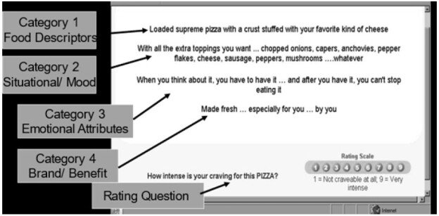
The research proceeded by mixing together these messages according to an underlying set of recipes, the so-called experimental design (REF). Figure 1 shows an example of the stimulus. The respondent did not see the boxes at the left, but simply saw combinations of elements, the messages, shown in the center of Figure 1. The respondent’s task was simply to read the vignette, and assign a rating. The task required the respondent to read and evaluate 60 different combinations, a task which took 10-12 minutes. Although the array of combinations, the so-called ‘vignettes’ seems like a set of randomly constructed combinations, the reality was and remains that in these Mind Genomics experiments great care is taken to create systematic combinations, each combination or set of 60 vignettes different from every other set, and each vignette comprising precisely the correct set of combinations to allow analysis by OLS (ordinary least-squares) analysis, even at the level of the individual respondent [5]. This design is called a permuted experimental design.

fig 1

Figure 1: Example of a vignette

To the respondent, the test combinations may appear to be haphazard combinations of messages the respondent was simply asked to read the combination, and rate the combination. The rating was ‘How intense is your craving for this FOOD NAME HERE IN CAPS). Most respondents looking at Figure 1 (without the call outs, but simply with the material present on the screen) begin by trying to ‘give the right answer’, but in the end the task to discern the pattern gives ways to a pattern of ‘read and rate.’ For the most part the respondent pays attention, but is not engaged in the task. The respondent is doing the task, but with little clear involvement, something which occasionally worries the researcher who would rather see a deeply engaged respondent. It is hard to be engaged when one has to evaluate 60 of these systematically created vignettes, but respondents do it, especially when they are motivated by rewards. The pattern makes it impossible for the respondent to game the system; Mind Genomics uses the statistical discipline of experimental design to create the combinations. When the study with 30 foods was done in 2002, the design used then was the so-called 4×9. The 4×9 design called for four silos or questions, each silo or question populated by nine different answers, or elements. The underlying experimental design called for 60 vignettes for each respondent, most comprising four elements, some comprising three elements, and some comprising two elements. Each respondent was given a different, permuted set of combinations, so that the combinations cover a great deal of the design space (rather than focusing on a narrow set of combinations, reducing the variability around those combinations, assuming those combinations are the correct ones to investigate.

The expectation was that the respondent would respond most strongly to the elements in Category 1 (product features), and perhaps secondly, to elements in Category 4 (brand, benefit). It was not clear what would be the response to elements in Category 2 (situation, mood), and especially those elements in Category 3 (emotional attribute, hereafter call ‘taglines’).

With this introduction, we now proceed to the actual experiment. Keep in mind that the analyses of these data is really a reanalysis of the results almost 20 years later, bringing into the work experience from two decades, and the evolution of thinking about what these data mean. The focus here is no longer on the rest of the data, but rather on what can be learned from the data of Category C, the ‘taglines’ or the emotional elements. The study here focused on teens, a continuation of an earlier studier of the same type, dealing with adults, using the same material, but focusing on older respondents [6]. The work with teens at that time was part of the expansion of Mind Genomics across test populations, especially beyond North American adults. Research among teens was the first major effort in this expansion, with the focus beyond foods to entertainment such teen e-zines [7].

The study reported here moves beyond the simple report presented first in 2002 to the IFT (Institute of Food Technologists), and appearing in a cursory overview in the journal Appetite in 2009 [8]. Those early presentations were made to a world of researchers who had never seen the It! studies, and were presented with a superficial view of this new approach to understanding people. It suffices simply to present the study is brief, since there was nothing like these new-to-the-world It! studies.

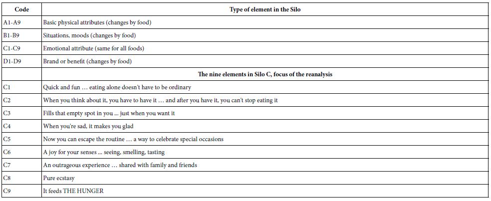
The analysis now focuses on the taglines, the nine emotion descriptors (C1-C9), previously considered minor. In It! studies these types of elements usually generated coefficients, utility values, hovering around 0, sometimes positive (viz., driving craving), sometimes negative (viz., not driving craving). In the interests of the science of that time, the formative years 2001-2005, these elements were ignore because of their poor performance in terms of their ability to drive rating ‘craving.’ With the increasing focus on clustering people with like patterns of response to these elements, and with the opportunity to compare the same elements across the many foods of the study, the reanalysis beckoned.

Method

Mind Genomics project are set up in a certain fashion, and analyzed to reveal patterns [9]. Over the years, the design has been modified made shorter Yet, despite the evolution towards simplicity, the Mind Genomics approach has become routinized, and the analysis made simpler, almost following a script [10]. The benefit of that ‘processization’ is that the research can focus on the data, the findings, and not on dealing method again and again. We present the process as the skeleton for reanalyzing the data.

Step 1: Choose the Foods to Study

Figure 2 shows the list of foods. Figure 2 comes from landing page to which the response is directed, for those respondents who choose to participate. As yet, the respondents do not know anything about the study. They are simply invited to participate, choosing the food they want. The objective was to have the respondent evaluate the foods that she or he liked. When the quota was filled (95 participants), the food and its button ‘disappeared’ from the screen, forcing the respondent to choose another food. The foods were the same as were used in the previous study, this time with adults [11].

fig 2

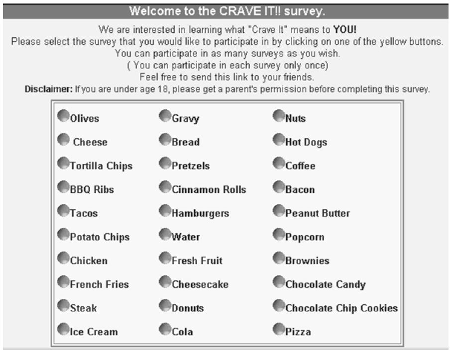
Figure 2: The 30 foods available for the respondent. The teen respondent went to the site, and chose the study which seemed most interesting

Step 2: Create the Design Structure and the Elements

The It! studies run 20 years ago were characterized by the 4×9 design, four ‘silos’ (categories in Figure 1) each with nine ‘elements’. The experimental design for Mind Genomics is set up to ensure that mutually incompatible elements are never allowed to appear together. That is the function of experimental design serves both a science role to allow for strong analysis at the level of the respondents (within subjects design) and a bookkeeping role to ensure that certain mutually incompatible combinations never occur, such as two different foods appearing together. Table 1 lists the key features of the 4×9 design.

Table 1: Key features of the design

table 1

Step 3: Combine the Elements into Vignettes, according to an Experimental Design

The typical approach espoused by researchers is to isolate the variable and study the variable in depth. The reality, however, is that the respondents don’t think about most things in their lives as being one-dimensional since meaningful things in their lives are combinations of features. If we want to learn about the relevance of each of the variables, the most practical thing to do is to systematically change the nature of the variables, creating several combinations, and then evaluate the combinations. This more practical strategy calls for experimental design.

The objective of experimental design is three-fold:

  1. Balanced, equal number of presentations of each element.
  2. Statistical independence, so that individual elements appear in a pattern making them statistically independent of each other, even at the level of the individual respondent. This first objective ensures that the data can be analyzed by OLS (ordinary least-squares) regression, at the level of the individual respondent, allowing for deep analyses. The ‘incompleteness of vignettes’ ensures that the coefficients emerging from the OLS regression possess the property of being absolute numbers, comparable across different studies.
  3. Bookkeeping, ensuring that mutually contradictory elements never appear together, such as two different stores in which the product is sold, or two different moods.

Step 4: Launch the Study, Collect the Ratings

Although there has been an ongoing effort to source market research respondents from individuals who volunteer their time (viz., using messages such as ‘your opinion counts’) the reality is that the studies are easier when one sources the respondents from company specializing in online research. These panel providers work with many respondents, and deliver respondents for a fee.

It is worth noting that the respondents were provided by a Canadian company, Open Venue, Ltd., in Toronto, Open Venue specialized in recruiting respondents for these types of online studies. It might seem more economical to recruit one’s own respondents, but the truth is that the study takes a very long time to complete. With Open Venue, and with the popular topic of food among teens, the 30 studies required a day or two to complete. The entire study took about three or four days in 2002.

The screening specifications were only about half males, half females, ages 16-20. The gender and ages were the proprietary information of Open Venue, Ltd. As is typically the case, the ages may have been somewhat out of date, so some respondents were older than their panel information would have one believe, simply because the ages were not updated every day.

The respondents were invited, went to the site shown in Figure 2. This first landing page invited the respondents to choose food. After the respondent chose the food, the respondent read the orientation page. All 30 studies began with the same orientation page, albeit individualized with the specific food name. The orientation page presents little information about the study. The reason for such paucity of information in the set -up is that the respondents are to be judging the food, and their craving for the food strictly on the basis of the information provided in the test vignette (Figure 2).

Figure 1 presents an example of a 4-element vignette, showing the category (viz., silo) from which, each element originates. The actual vignettes do not show the silo or the identification number of the element. Rather, the vignette simply shows the elements prescribed by the experimental design, in unconnected form. Having connectives in the vignette is neither necessary nor productive. Respondents inspecting a vignette do not need to have the sentences connected. They simply need to have the information available in an easy to discover way. Figure 1, in its spare fashion (without explanatory material with arrows), does just that.

Steps 5 and 6 – Create the Database Showing Respondent, Vignettes, Rating, and Answers to Classification Question

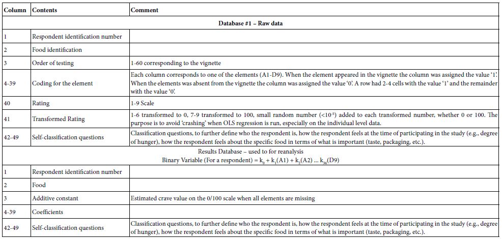
Mind Genomics is set up to acquire data in a structure, rapid, and efficient fashion, almost ready for statistical analysis after two transformations. Each respondent who participated was assigned a panelist identification number. The respondent’s data from the 60 vignettes were put into a database to which each respondent contributed 60 rows of data. Each row corresponds to a respondent and a vignette presented and evaluated. The Mind Genomics program constructed the vignettes ‘on the fly’ as the study was progressing, presented the stimulus, acquired the response, and populated the database, all in real time. The construction of the database appears in Table 2.

Table 2: Construction of Mind Genomics data for the Teen Crave it study

table 2

Step 7 – Result for Total

The database constituting the focus of our attention be the database emerging from the use of the OLS (Ordinary Least Squares) regression on the data of each individual. Thus, we will deal with 2000+ equations, and in the same form, different only by the respondent who generated the equation and the food. Our focus will be only on the coefficients of C1-C9, the tag lines as we have called them.

The rationale for focusing only on the tagline is that in study after study, these taglines never perform as well as the elements which describe the product. Yet, the advertising agencies focus on these elements. In previous studies of this type, and in virtually every study, the emotions, and taglines, so often felt to be important by salespeople, but technical people as well, score poorly. By ‘poor’ is meant low values for the coefficients. The ingoing explanation is that people focus on the food, and not on the feelings about the experience. In the worlds of poetess Gertrude Stein who opined for many objects and people ‘‘there’s no there there’. Certainly, there is a point to that statement since there is nothing about real food and real life in tagline elements, C1-C9.

Table 3 shows the summarized results of food (row) by tagline (column). The data come from the summary table of coefficients described in the bottom part of Table 2, dealing with the databasing of the summary models. The table presents only positive coefficients of 2 or higher. The negative and zero coefficients are not shown. Thus, these positive coefficients are those which drive craving. The coefficients in Table 3 are averages from all of the respondents who participated in the particular study. All coefficients of 8 or higher are shaded, corresponding to the fact that these coefficients are statistically significant (p<0.95).

Table 3: The foods and the elements, showing only those combinations with coefficients 2 or higher. The foods are sorted in descending by the sum of the coefficients across the elements. The elements are sorted in descending order by the sum of the coefficients across the foods

table 3

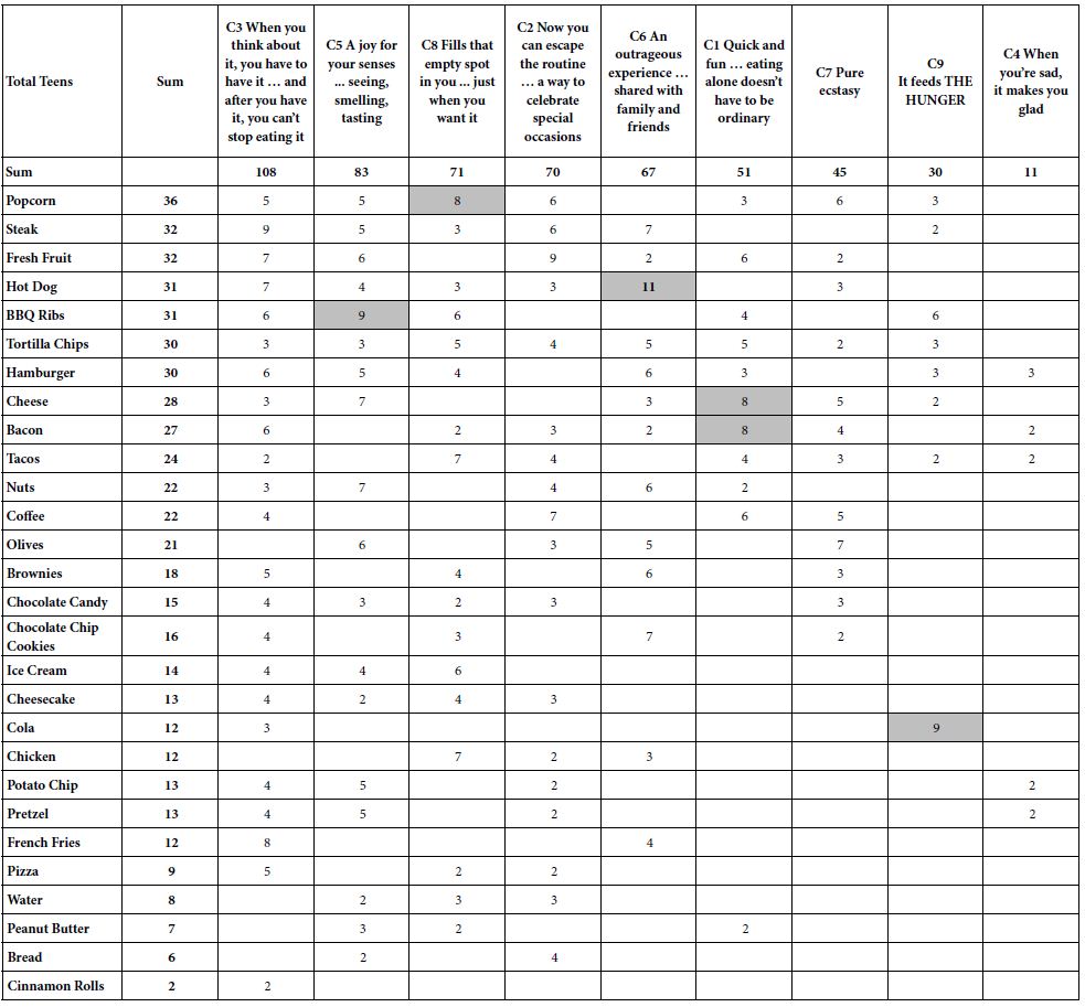
The foods are sorted from top to bottom by the sum of the positive coefficients (+2 or higher), as shown in Table 3. Thus, the food with the highest sum of coefficients is popcorn, the lowest is cinnamon rolls. Then the columns are sorted from left to right in descending order, so that the element with the highest sum of coefficients (When you think about it, you have to have it … and after you have it, you can’t stop eating it) is at the left, and the element with the lowest sum of coefficients is at the right (When you’re sad, it makes you glad).

The table as constructed from the Total Panel provides virtually no insight, except for the observation that only six elements generate coefficients of +8 or higher, and only among one of the nine tagline elements, C1-C9. It should come as no surprise that for virtually of the It! studies reanalyzed during the past 20 years, these ‘tag lines’ have been discarded, because they seem not to have any profound insight about the mind of the respondent. The coefficients are low, and even when they are studied together with other elements, such as the names of foods, and the health benefits, these ‘tag lines’ seem to vanish into irrelevance. Parenthetically, it would take 20 years, and a separate way of thinking about Mind Genomics data of this type, in a specific format, to provide the impetus to reanalyze the data, and to reveal new findings and patterns reported here.

Step 8 – Results by Gender

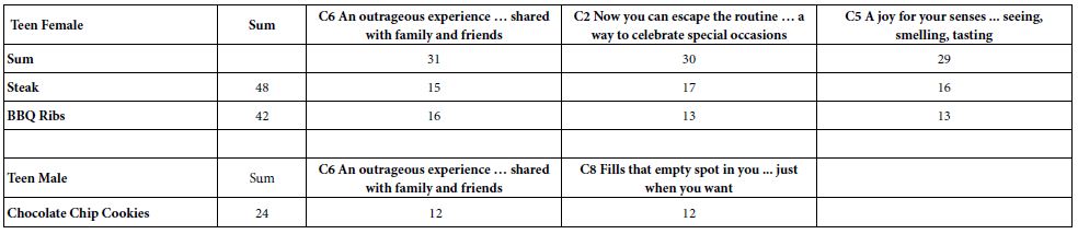
Respondents classified themselves by gender. Thus, it was straightforward to compute the average for each of the nine elements by gender and by food. Rather than total, we present the results for by gender. When we separate the respondents by gender we have many more elements with positive coefficients. The patterns are easier to discern when we retain for consideration only those average coefficients of 10 or higher, for a specific gender/food/element combination. The other averages, 9 or lower, are eliminated from the table. We also eliminate any element whose sum of positive coefficients is 23 or lower. (Parenthetically, the original cut-off point for sum of positive coefficients for an element was 24 or lower, but that would have eliminated males.

Table 4 shows a dramatic pattern. Teen Females show far more strong performing combinations, and the magnitudes of the coefficients are higher. The difference is simple. Teen females appear to crave meat; teen males appear to crave chocolate and sugar.

Table 4: Strongest cravings for genders based upon the tag lines

table 4

Step 9 – Results by Self-rated Hunger at the Time of Participation

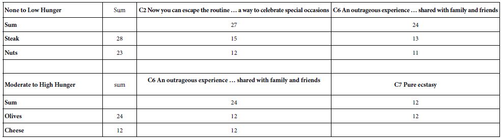
The respondents were instructed to rate their hunger on a 4-point scale. Table 5 compares the coefficients for the elements by food, again showing only coefficients which are 10 or higher. Unexpectedly, few foods show strong coefficients for the taglines, perhaps because there may be other elements, such as food description, which are more salient when a respondent is hungry. When we look through the lens of the tag line, we see only three emerging. For those with low hunger the foods are steak and nuts, and the taglines are celebration. For those with moderate to high hunger the only element which really satisfies the requirement is an olive, perhaps because of the noticeable salt taste.

Table 5: Strongest cravings during hunger state, based upon the tag lines

table 5

Step 10 – Identify Mind-sets in the Population Showing different Patterns of Coefficients

A hallmark of Mind Genomics is the discovery of mind-sets, similar patterns of responses to elements from respondents who seem otherwise not related to each other by the pattern of their self-described profiles in a classification questionnaire. Typically, a study may generate 2-3 mind-sets when the topic is multi-faceted. More mind-sets or clusters can be generated but with the increasing number of mind-sets the power of the clustering decreases because the results become increasingly harder to use.

The clustering here is done independent of the specific food, viz., incorporates all of respondents into one dataset, and clusters that dataset. The only information used for the cluster is the set of nine coefficients. Furthermore, those respondents whose coefficients were all 0 for the nine coefficients were eliminated ahead of the clustering, because they showed no pattern of differentiation among nine tag line elements, C1-C9.

The k-means clustering program computed the pairwise ‘distance’ between each pair of respondents, by computing the Pearson correlation. The correlation, in turn, is a measure of the strength of a linear relation, with a high of +1 to denote a perfect linear relation between the coefficients of two respondents, down to a 0 to denote no relation, down to a low of -1 to denote a perfect inverse relation. The distance (defined as 1-Pearson R) goes from a value of 0 when two respondents show perfect correlation in their coefficients, up to a value of 2 when two respondents show perfect inverse correlation [12].

The clustering was done on the nine coefficients for each respondent, independent of the specific product the respondent was evaluating in the Mind Genomics experiment. Each respondent generated additive constant and 36 coefficients, one for each element. The analysis kept only the coefficients C1-C9, which constitute the focus of this analysis. In most Mind Genomics studies the deconstruction of the respondent population into mind-sets allows the different, often opposite-acting groups, to emerge. The groups no longer cancel themselves out. This can be said for the mind-sets developed out the tag lines. Table 6 shows three clearly different groups, with higher coefficients for the different foods. Furthermore, the groups make intuitive sense.

Table 6: Strongest cravings during hunger state, based upon the three emergent mind-sets

table 6

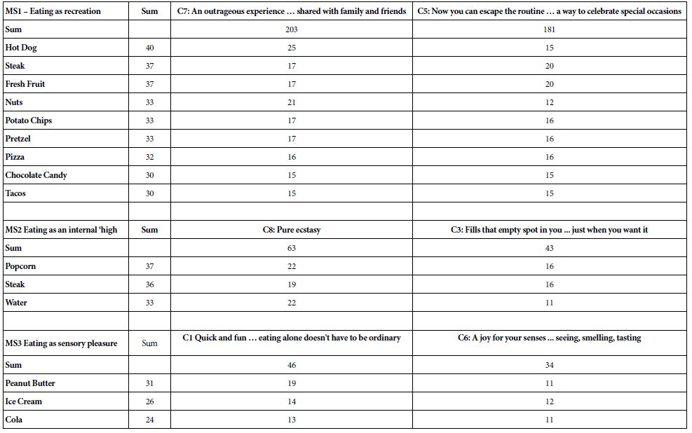
MS1, Mind-Set 1, appears to respond to elements C7 and C5, focusing on eating as recreations. The foods make sense.

MS2 appears to response to elements talking about an internal strong response, a ‘high’. The foods are unexpected, popcorn, steak, and water, respectively. The reason for this is not obvious at this time.

MS3 appears to respond to elements about eating as sensory pleasure. The three foods are all laden with sugar and are soft in text or even liquid; peanut butter, ice cream, and cola.

Classification

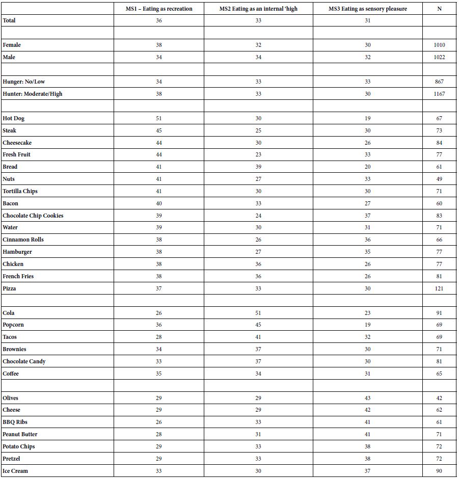
Table 7 presents the classification of respondents into the three mind-sets, by total, then by gender, self-reported hunger and food, respectively. There are patterns of mind-sets vs. food, e.g., for hot dog 51% of the respondents fall into MS1, whereas for cola 51`% of the respondents fall into MS2, and for olives 43% fall into MS3. There are no clear patterns, but the Mind Genomics approach permits the researcher to move beyond the conventional psychographic clustering often heralded as a major advance beyond clustering based upon geo-demographics [13].

Table 7: Distribution of the three mind-sets by key groups (total, gender, self-reported hunger, food study in which the respondent participated)

table 7

Discussion and Conclusions

The original analysis for the Crave It! studies focused on the strongest performing elements, looking at the different foods, as well as the different groups within each study, specifically gender. The effort to discover mind-sets had originally motivated all of the It! studies, the Teen Crave It! no different than any of the others.

The results of the early studies revealed that the respondents divided most strongly on the response to the food and to the eating experience. The ‘tag lines’, shown in Table 2, were low in comparison to the coefficients for the different foods and in each study. Again and again, the foods themselves and the eating situations showed double-digit positive coefficients, and an occasional negative coefficient. The obvious conclusion at that time was that the tag lines are unimportant, at least during the early 2000’s when the It! studies were run.

The observation leading to this paper was not so much an observation as a question. The question was simply ‘what would happen if we were to look at the coefficients of the tag lines’, not from the total panel, but broken out into foods, gender, stated hunger, and even use the coefficients of these tag lines (C1-C9), alone, by themselves, to generate mind-sets? The decades of experience of with Mind Genomics had revealed, again and again, that the simple and rather startling result that of coefficients around 0 often hid profound, interpretable, and instructive differences between groups, occasionally differences that could be labelled ‘remarkable.’

The analysis with the tag lines reveals a world of insight lurking below the surface of these relative low coefficients, doing so for elements which do not at the surface pertain to food in the way that food names and eating situations do (Elements A1-A9, and elements B1-B9).

The most difficult part of the analysis was to enable the discovery by paring away the extra numbers. It is one thing to pare away noise which is clearly noise, elements which are negative or close to zero. The focus is on the food. The elements which score high with regard to that food, especially on the rated attribute of craving, allow the pattern to come through. In this analysis, however, we are searching for a more amorphous pattern, not one easily observed. The issue becomes to create criteria which allow fair elimination of a lot of the data, without so-called ‘p-hacking’ or searching for effects, and then claiming those effects to have emerged as reportable outputs from the study and expressed within the original hypothesis. For these data the discovery of the patterns is a matter of paring away different sets of coefficients, pertaining either to foods (rows) or elements (columns), so that the underlying pattern makes sense. That approach, subjective in nature, consists of eliminating foods which generated low coefficients across elements, and eliminating elements which generated low coefficients across foods do so in an iterative fashion until the patterns become stable, and the story emerges, perhaps even compelling.

Thus, the analysis closes; the ‘story’ now expands to promote the relevance of tag lines as a new way to understand the mind of the consumer in the case thinking about foods. It may be these taglines, almost throwaway, amorphous statements, which provide new insights. In a sense, the tagline becomes the screen onto which the other aspects of the respondent’s mind are projected; witness the emergence of the three mind-sets.

References

  1. Pilgrim FJ, Peryam DR (1958) Sensory testing methods: A manual (No. 25-58). ASTM International.
  2. Harvey K, Kemps E, Tiggemann M (2005) The nature of imagery processes underlying food cravings. British Journal of Health Psychology 10: 49-56. [Crossref]
  3. Tiggemann M, Kemps E (2005) The phenomenology of food cravings: the role of mental imagery. Appetite 45: 305-313. [Crossref]
  4. Weingarten HP, Elston D (1991) Food cravings in a college population. Appetite 17: 167-175. [Crossref]
  5. Gofman A, Moskowitz H (2010) Isomorphic permuted experimental designs and their application in conjoint analysis. Journal of Sensory Studies 25: 127-145.
  6. Moskowitz H, Silcher M, Beckley J, Minkus-McKenna D, Mascuch T (2005) Sensory benefits, emotions and usage patterns for olives: using Internet-based conjoint analysis and segmentation to understand patterns of response. Food Quality and Preference 16: 369-382.
  7. Moskowitz H, Itty B, Ewald J (2003) Teens on the Internet-Commercial application of a deconstructive analysis of ‘teen zine’ features. Journal of Consumer Behaviour: An International Research Review 3: 296-310.
  8. Foley M, Beckley J, Ashman H, Moskowitz HR (2009) The mind-set of teens towards food communications revealed by conjoint measurement and multi-food databases. Appetite 52: 554-560. [Crossref]
  9. Moskowitz HR, Gofman A, Beckley J, Ashman H (2006) Founding a new science: Mind Genomics. Journal of Sensory Studies21: 266-307.
  10. Biró B, Gere A (2021) Purchasing bakery goods during COVID-19: A Mind Genomics cartography of Hungarian consumers. Agronomy 11: 1645.
  11. Moskowitz H, Beckley J, Adams J (2002) What makes people crave fast foods?. Nutrition Today37: 237-242.
  12. Likas A, Vlassis N, Verbeek JJ (2003) The global k-means clustering algorithm. Pattern Recognition 36: 451-461.
  13. Wells WD (2011) Life Style and Psychographics, Chapter 13: Life Style and Psychographics.

Characterization in Adolescent from Families’ Consumers of Alcohol in a Community of Health

DOI: 10.31038/JCRM.2021433

Abstract

Context: To improve the life styles from the Cuban community context of family health is a reality linked with the medical sciences.

Objective: To characterize in adolescents from families consumers of alcohol in a community of health. This process embraced the period of September 2018 to June 2019. The qualitative methodology was used, with a descriptive and traverse study. The universe the 45 adolescents in families of studies, selected in an intentional way.

Methods: Observation, interview and revision of clinic history and the techniques were: test of family operation.

Results: It was evidence that toxic styles of life exist. The male sex was the more affected for 56% by alcoholic relatives. The most frequent causing lifestyles of family dysfunction were the daily ingestion of alcoholic drinks.

Conclusions: The families present difficulty in the family relations. The addiction to the alcohol is related with the tolerance and consumed by day that it generates in the life style from the family operation.

Keywords

Alcoholism, Adolescent, Addiction, Family relations, Styles of life, Health

Introduction

The family is the most important social group in any society, it is the place where the formation of the personality begins and where the affections are committed with the interactions among their members. The economic, biological, educational and satisfaction functions of affective and spiritual needs that the family group plays are of marked importance because, through them, values, beliefs, knowledge, criteria and judgments that determine the health of individuals and the collective are developed and its members; a disease such as alcoholism in one of its members affects the dynamics of this family group. The World Health Organization (WHO) defines alcoholism as a disease characterized by the excessive and frequent ingestion of alcoholic beverages whose consumption can cause the phenomena of tolerance and dependence that cause biological, psychological and social damage in the individual [1,2].

Alcoholism is a chronic disease that damages the organism, family and social functioning and can be a cause of violence, antisocial behavior, family disagreements, accidents and even homicides. The best places to avoid the excessive consumption of alcoholic beverages are the family and the community, because there the individual must learn healthy lifestyles, among which the excessive consumption of alcohol does not enter. The addiction continues being a dysfunction caused by a substance able to produce dependence, the alcohol. In the medical sciences the health is defined as the state of beneath bio psychosocial and spiritual and not the absence of illnesses. The addiction continues to be a dysfunction caused by a substance able to produce dependence, the alcohol. In the medical sciences the health is defined as the state of bio psychosocial and spiritual and not the absence of illnesses. Adolescence is a stage of life between childhood and adulthood that is intimately related to both since many characteristics of the previous stages are present with other new ones evidenced until then. In adolescents, alcohol consumption is often associated with fun, self-determination, leisure and modernity and constitutes an element that gives status to their group of members, which makes it more difficult to eliminate them despite negative consequences derived from excessive consumption. For teenagers, among whom the most popular drug is alcohol, this is undoubtedly a dangerous drug with consequences that can endanger life; hence it is called drug porter and model [3-5].

Cuba, do not escape this problem. Research studies have been conducted where a significant number of adolescents are at risk of becoming alcoholics at some point in their adult lives; hence it was decided to conduct a study aimed at knowing if the functioning of the families of adolescents’ risk of alcoholism influences his behavior before this toxic. In such a sense thinks about the following scientific problem: How characteristic it presents the adolescents from families’ consumers of alcohol in a community of health? The general objective that thinks about is to characterize in adolescents from families consumers of alcohol in a community of health.

Methods

The families was carried out a descriptive study, traverse with adolescents from a context of community family health of the municipality Santa Clara, Cuba in the understood period of September 2018 to June 2019, with the objective to characterize in adolescents from families consumers of alcohol in a community of health. It was study object a universe constituted by 45 adolescents and families of studies, selected in an intentional way. Methods of the theoretical level: Analytic synthetic: It facilitated the interpretation of the texts and to establish the corresponding generalizations. Inductive-deductive: facilitated to go of the peculiar to the general thing in each one of the analyses carried out in the theoretical study. Generalization: It allowed the establishment of the regularities that showed in the carried out study.

Empiric Level

Revision of Family Records

It constitutes a legal document, doctor and official zed of great personal and acquisitive value, to be registered the entire relative one prior to the clinical history of the family, gathering and obtaining more reliable and richer information for the investigation.

Clinic History

It is applied with the objective of measuring the indicators that influence teen alcohol consumption.

Test of Family Operation

It is applied with the objective of measuring the level and incidence of some determinant of the health in the context of the family, talkative relationships and life styles.

Inclusion Approaches

I. Adolescents with families’ consumers of alcohol.

II. That they resided in the area of chosen health.

Exclusion Approaches

III. Families that emigrate of their residence place during the study.

Exit Approaches

IV. Adolescents and families that abandon the investigation voluntarily.

Statistical Analysis

The information was stored in a file of data in SPSS version 12.0 and it is presented in statistical chart; for the description it was calculated with the method statistic of Fisher.

The absolute and relative frequencies were determined. For the analysis of the qualitative variables, the X² statistic was used to determine the independence between factors and for goodness of fit with a level of significance α = 0.05; there are significant differences when ρ<0.05 and not significant when ρ>0.05.

Results

Chart 1 refers to indicators according to behavior and sex, where it was appreciated that the most common reason was the group contagion given in a typical camaraderie code of this psychological age represented by depression (97,6%), followed by the presence of frustration feeling (75,6%) and undervaluation with 70,7%.

Chart 1: Distribution of adolescents according to indicators of behavior and sex

Indicators of the behavior in adolescents

Sex

Female

Male

Total

No.

% No. % No.

%

Depression

11

91,6 29 100,0 40

97,6

Frustration feeling

9

75,0 22 75,9 31

75,6

Undervaluation

8

66,7 21 72,4 29

70,7

low self-esteem

8

66,7 20 68,7 28

68,3

Anxiety

5

41,7 14 48,3 19

46,3

Group imitation

3 7,3 3

7,3

Source: Clinic history

It is important to highlight that adolescents who feel depressed have a high probability of consuming alcohol as aversive way, which was reflected in the present work, where 68,3% of the subjects admitted that they had done it for causes of low self-esteem.

Discussion

Among the students surveyed, an average age of 13 years was observed, with a greater predominance for males, which coincides with other studies related to psycho-affective and social disorders in adolescents with alcoholic relatives. These results can be justified because at this stage of life adolescents feel invulnerable and assume omnipotent behaviors, almost always generators of risk; In turn, the school group in which it operates has great influence and its behavior will be highly influenced by the opinion of the same when making decisions and undertaking a task. The group constitutes a way of transmitting norms, behaviors and values that, on occasions, is more influential than the family itself. In such a sense the members of the family should contribute with appropriate attitudes to the improvement of an effective communication that allows a dynamic and systematic. The majority of adolescents presented several situations prone to consume alcoholic beverages, which justifies inadequate coping styles that adversely affect family functioning and their integral health. Family arguments and domestic violence are an impediment to the adolescent’s training and, at the same time, situations that tend to give the adolescent a risk behavior when faced with alcohol consumption. In many cases one of the members of the family was a consumer of alcohol, which is a factor that triggers stress and changes in family functioning. Similar results were found when reviewing the studies of several authors in the country that consider alcoholism, together with conflicts in the family nucleus, as a risk factor of considerable value for families to lose their structural and functional stability. Great social impact has the fact that adolescents are deformed in their behavior, caused by the family environment, it was shown that the ingestion of alcoholic beverages is an important factor causing family dysfunction [6-12].

For the majority of adolescents alcoholism is not a disease, only a low percentage of them recognize it that way, so the little perception of risk that the studied patients present is worrisome, although most of them see it as a drug, a vice, a dependency and a bad habit; It is alarming that many of the adolescents see it as a way to share with friends, as a feature of manhood and as a pleasure, all linked to the risk factors present in these families. In adolescents, alcohol consumption is often associated with self-determination, fun, leisure and modernity and constitutes an element that gives status to their group of members, which makes it more difficult to eliminate them despite the consequences negative consequences of excessive consumption and not to consider it as a scourge that harms human values. Many authors have studied the family dynamics in the home of origin of the alcoholic and point out the coincidence of several alterations when they characterize the children and adolescents who live with these patients. Many of the children who have behavioral difficulties grow up in an inadequate family environment and learn to survive, although not to thrive. Children raised in such circumstances arrive at school without possessing experience, nor the necessary aptitude for a methodical instruction and they do little in school [13,14].

Conclusions

Keeping in mind the individual values and the reference group to that belong, for what becomes necessary to carry out strategies educative that allow a well-being bio psychosocial and spiritual to these adolescents coming from families dysfunctional. Although these adolescents come from families dysfunctional he biggest percent they are independent, this can be associated to that the adolescence is a stage difficult of the development where the independence can be favored, the freedom in the taking of decisions or the imitation to the adults from the family operation. By way of conclusion according to like the internal and external conditions are developed starting from the interaction with the diverse subjective configurations from the family context. The families present difficulty in the family relations. The addiction to the alcohol is related with the tolerance and consumed by day that it generates in the life style.

Conflict of Interest

The author declares no conflict of interest

References

  1. López RM, Quirantes MMJ, Pérez MJA (2006) Pesquisaje de alcoholismo en un área de salud II. Rev Cubana Med Gen Integr 22: 2
  2. Colectivo de autores. Alcoholismo, Cuida tu salud. Cuba, Ciudad de la Habana: Edición Digital; 2006.
  3. Barnow S, Schuckit MA, Lucht M, John U, Freyberger HJ (2002) The importance of a positive family history of alcoholism, parental rejection and emotional warmth, behavioral problems and peer substance use for alcohol problems in teenagers: a path analysis. J Stud Alcohol 6: 305-15. [crossref]
  4. García PRP, Toribio MA, Méndez SJM, Moreno AA (2004) El alcoholismo y su comportamiento en cinco Consultorios Populares de Caracas en el año. Med Gen 187: 522-28.
  5. Gruenewald PJ, Russell M, Light J, Lipton R, Searles J, et al. (2002) One drink to a lifetime of drinking: temporal structures of drinking patterns. Alcohol Clin Exp Res 26: 916-25.
  6. Sánchez CME, Ramírez TA, González ED, Castellanos VE, Ojeda RJ (2006) Trastornos psicoafectivos y sociales en adolescentes con familiares alcohólicos. Rev AMC 10: 1
  7. González R (2005) Secretos para prevenir, detectar y vencer las drogadicciones. La Habana: Científico- Técnica.
  8. Bolet AM (2000) La prevención del alcoholismo en los adolescentes. Rev Cubana Med Gen Integr 16: 406-409.
  9. Martínez HAM. (2008) Alcoholismo, hombre y sociedad. 2da parte y final. Adicciones, Salud y vida.
  10. Ortiz GMT, Louro BI. Jiménez CL. Silva ALC. (1999) La salud familiar.Caracterización en un área de salud.
  11. Pereira JI, Sardiñas Montes de O. (1999) Comportamiento de la violencia intrafamiliar sobre adolescentes en un área de salud. Rev Cubana Med Gen Integr 15: 3
  12. Mancilla C, Pereira C (2002) Un estudio de factores psicológicos, socioculturales e individuales. Chile: Universidad Valparaíso.
  13. Otaño FY, Valdés RY (2004) Algunas reflexiones sobre el alcoholismo en la comunidad. Rev Cubana Enfermer 20: 3.
  14. Sánchez MA (1998) Modalidades de conducta ante el alcohol en adolescentes. MEDISAN 2: 3.

Late Life Depression: Review of Perception, Assessment and Management in Community Dwellers

DOI: 10.31038/ASMHS.2022613

Abstract

Depression is one of the mental health conditions identified and projected to be the second leading cause of burden of disease in late life and unfortunately concerns for its debilitating consequences have birthed the need for continuous studies into its etiology, risk factors and management options (WHO, 2017). As the world aged population increases (by 2 billion persons in the next 30 years from 7.7 billion currently to 9.7 billion in 2050), number of older adults aged 65 years and over is projected to proportionately grow by 50% from about 727 million in 2020 to more than 1.5 billion by 2050 (United Nations, 2020) invariably implying that one in six people worldwide will be aged 65 years and over. Averagely, the number of older adults manifesting symptoms of mental disorders such as depression is set to increase proportionately among the estimated population.

The sudden but precipitated increase in incidences of depression across all ages had necessitated the need for constant reviews of mental health disorders. Factors that informed the mental health decisions of community dwelling older adults are hinged on their personal convictions on the presence of the disease and not just another somatic related illness. These convictions are quite germane to the kind of treatment they sought for and could invariably be the major reason why geriatric depression has consistently been misdiagnosed or undertreated very often among community dwelling older adults.

Keywords

Late life depression, Mental health, Burden of disease, Community dwelling older adults

Introduction

Depression is one of the mental health conditions identified and projected to be the second leading cause of burden of disease in late life and unfortunately concerns for its debilitating consequences have birthed the need for continuous studies into its etiology, risk factors and management options across all populations and samples [1]. As the world aged population increases (by 2 billion persons in the next 30 years from 7.7 billion currently to 9.7 billion in 2050), number of older adults aged 65 years and over is projected to proportionately grow by 50% from about 727 million in 2020 to more than 1.5 billion by 2050 [2] invariably implying that one in six people worldwide will be aged 65 years and over. Averagely, the number of older adults manifesting symptoms of mental disorders such as depression is set to increase proportionately among the estimated population. Good news however is that mental health issues in late life has been explored within different population of older adults globally.

Specifically, literature exploring late life depression in community samples and in clinical trials have been widely explored [3-7]. Though comparison in case reports from continents varies as limited number of accounts of depression among older adults in Africa constitute a major setback in reports and management [7]. Despite the disparities in reports and studies conducted all over the world, the goal of research in bridging gaps in findings had been successfully achieved; studies had established the etiology of late life depression, consequences of untreated depression and management options had also been widely appraised. This review will address types of depression relative to older adults, diagnosis and complications of undiagnosed late life depression, the interpretation and assessment of depressive symptoms and experience of depression in some Nigerian communities will also be explored. Publications on the psychological management and implications of culture on the expression of depression in community samples of older adults will also be appraised in relation to their clinical and research implications.

Late Life Depression

Psychological issues have remained an issue met with lots of reluctance and ignorance which older adults are always embarrassed to describe. Presentation of depression in late life which often include insomnia (complaints about difficulties in recall and identification), social withdrawal (lack of interest in social activities and behavioural changes characteristic of hostility (irritability), frequent unexplained falls, hallucination, agitation etc. are often missed for age-related illnesses or somatic complaints [8]. The Diagnostic and Statistical Manual of Mental Disorders (DSM–5), gave a clear description of Major Depressive Disorder (MDD) as: “a manifestation of multiple major depressive fits”. A depressive fit is described in the DSM-5 as mood change characterized by variations in emotions resulting in a continuous manifestation of multiple characteristics of depressive behaviours usually exhibited concurrently for two weeks. Other accompanying symptoms may include daily display of a characteristically low emotional state observed either by the sufferer or observation made by others [9]. Anhedonia, described as an identifiable attention shift from all or from about all activities of choice, spanning throughout the day or on daily basis. Drastic loss or gain of body weight, daily amnesia or hypermnesia [10], daily mental degeneration, daily burnout (feeling stressed), excessive or inappropriate self-attribution of guilt and or cognitive retardation [11].

There must be an accompanying diagnosable distress or discomfort and social withdrawal following the listed symptoms to meet the criteria of the DSM-5. Of the five symptoms, the sufferer must either have a “depressed mood” or totally lose interest in pleasure or social activities. Other symptoms typical of late life depression include somatic complaints, cognitive impairment, persistent anhedonia or loss of pleasure, behavior changes and the pronounced presentation of negative personality traits [12,13]. There has been an age long societal misconception about aging and its accompanying misery. Coincidentally, this reflection has been documented in literature, myths and beliefs of people across diverse communities all over the world [9]. [14] in his argument for the inclusion of counseling sessions in the proper diagnosis and treatment of age related physical and mental illnesses established that many physical manifestations of late life depression could mimic the symptoms of illnesses peculiar with old age making depression diagnosis relatively difficult [10].

Depressive Disorders in Late Life

Major Depression

Major depression, also referred to as depression is a mental health disorder characterized by at least two weeks of consistent negative mood swings observed across the individual’s activities of daily living. It is characterized by poor self-esteem, loss of interest in normally enjoyable activities, fatigue, and bodily ache [15]. There is a close similarity between the DSM-IV-TR [16] criteria for major depression in both old and younger individuals and the DSM-5. Major depression in older adults may be preceded by cognitive impairment that may develop after the onset of depression, this condition is described in [17] as dementia syndrome of depression, because of the obvious cognitive deficits.

Vascular Depression

Vascular depression is the comorbid presence of heart related complications in depressed older adults diagnosed with their first onset of depression [18]. There is the hypothesis that manifestation of late life depression with associating vascular risk factors is complicating to both the sufferer and the clinicians. The risks of misdiagnosis for clinicians are higher, medication interference, and nihilistic attitude from the patient are all compounding for vascular depressive patients [19].

Psychotic Depression

Clinically diagnosed psychotic depression is any form of depression associated with physical characteristics like hallucination, delusions and violent agitation. Psychotic depression is most common in late life; it includes many difficult to treat symptoms like hallucinations, delusions paranoia, and weight loss due to not eating and dehydration due to not drinking [20].

Dysthymia

Late onset of dysthymia in late life have a higher prevalence and comorbid factor of cardiovascular disease but are otherwise similar to older patients with late onset depression [21]. Dysthymia is a psychological disorder with presenting symptoms closely mimicking depression with a repeated occurrence lasting through several days or years. Dysthymia is associated with the risk of the development of major depression in older adults, so-called “double-depression,” and may be particularly treatment resistant [18].

Diagnosis and Complications Late Life Depression

Depression assessment for older adults can be challenging, especially in the physically frail and cognitively impaired. Coexisting medical conditions typical with old age can increase older adult’s susceptibility to depression [22]. Proper assessment to rule out the possibilities of other physical health conditions such as hypothyroidism, alcohol use, incontinence, falls, partial and total stroke, cardiac related issues, drug abuse etc. that may contribute to depression need be done before the major depressive disorder diagnosis [23]. Researchers and caregivers are daily challenged on the choice of assessment techniques, diagnosis and identification of depression pointers. For clinicians working with older adults, identifying the prognostic consequences of comorbid medical illnesses in geriatric depression is essential to management and treatment planning [20]. These accompanying medical illnesses poses great difficulties in diagnosing depression having established the interference of medical conditions overlapping affective disorder symptoms. Clinicians must attain a balance when assessing older adults for depression between assumptions [24] (misunderstanding the psychomotor decline in Parkinson disease for a depressive disorder) and outrightly exclusive (erroneously dismissing an older adult’s mood swings as “understandable” and typical with old age).

Additionally, for the geriatric population, a number of medications are believed to have interactive effect on their emotions and psychological dispositions thereby igniting a depressive disorder. Use of prescribed medications in old age if not religiously taken may have associating consequences [10]. Depression is a state of emotional disequilibrium which can be managed with clinically prescribed antidepressants. Antidepressant use is known to have a higher interference effects with other medications prescribed for use in old age. [25] reported that sampled cases, market survey reports and reflective studies have carefully examined the relative effects of medications like antipsychotics, corticosteroids, endocrine-altering medications, stimulants etc. with late life depression. Other factors hindering proper diagnosis of geriatric depression may include poor and incoherent communication skills in the elderly [24], presence of multiple somatic complaints not well expressed (Isabella & Henrietta, 2008), time constraints during clinical visits among others.

Geriatric depression left untreated or undiagnosed predisposes older adults to chronic effects of the disorder. Complications of untreated geriatric depression identified in literature may include:

Worsening Emotional Well Being

Old age is presumably a time when older adults are assumed to observe lots of fun activities to relieve already suppressed emotions. It is presumed to be a time to reminiscence and relish the accompanying relief of leaving an active phase of life. Unfortunately, aging and its accompanying complexities are not always perfect as assumed. Sporadic turn of events accompanying physical frailty, systemic degeneration, osteoporosis, incontinence etc. are not in totality very tolerable, they tend to weigh heavily on older adult’s psychological disposition [27]. Geriatric depression is a psychological disorder that requires a balance in cognition, attitude and genetic composition. Older adult’s inability to maintain a balanced emotion are at a greater risk of having a depressive episode with its associating risk factors [28].

Suicidal Ideation, Act and Behaviour

Suicide is unarguably the commonest and an extreme psychiatric emergency [29]. The World Health Organization (2000) definition of suicide as a self-attempt to kill and deliberately terminate life initiated and orchestrated by the individual having a full knowledge of the consequences and fatality is just a total summation of the act and its consequence. [30] in their documentation of the incidence and prevalence rates of suicide in the geriatric population presented a figure that is non-comparable with the younger population across most countries. Expressively implying that older adults are at a greater risk of death by self-suicide than the younger population. For every suicide attempted, the margin of those successfully completed is higher in the geriatric population as with a suicide reported in about twelve attempts, four will be effectively completed [31]. In other words, suicide attempts among the geriatric population should be seen as a serious health concern.

Reports on suicide and suicidal attempts in Nigeria taking instances from the stories of an unidentified medical doctor’s suicide on the Third Mainland Bridge in Lagos reported by [32], the story of a final year student of Ladoke Akintola University of Technology, Ogbomosho, with a ‘First Class’ who died of self-poisoning, a woman reported to have been rescued from suicidal attempt on the same mainland bridge who confessed to hearing voices calling her to come to the bridge and jump etc. The disappointing part of these stories which foregrounds the difficulty in tackling depression-induced deaths was the comment of an unnamed friend of the medical doctor whose case seemed to be most recent, about the deceased being very funny and lively [24]. In advanced stage of depression especially in older adults, they cover up with laughter and tend to be extroverted when around people so as to hide deeper psychological ‘injury’. Sadly, this type of comment follows virtually every case of suicide reported in Nigeria, [32]. Psycho-pathologically, in a deeply cultural and religious Nigerian society where awkward death by suicide are never taken as a possible negative response of mental disorders, it is not surprising to see people attributing suicide to witchcraft. While the possibility of such a cause cannot be entirely ruled out due to the deep connection Nigerian society shares with religious rites and the belief in metaphysical powers, the fact that it cannot be scientifically proven makes it unreliable [33].

Interpretation and Assessment of Depression in Some Nigerian Communities

Owing to the diversities in culture and traditions in Nigeria, clinicians and medical professionals have reported ethnic variances in reporting and diagnosing geriatric depression. [34] in his report of the nature and diagnosis of depressive disorders in Nigerian elderly highlighted differences in older adult’s expression of depression based on cultural diversities, religion and social groupings. Over sixty percent of the Nigerian population will readily employ the services of traditional healers before consulting the conventional medical experts. This submission reported by [35] alluded to the general consensus that traditional or alternative medicine is widely perceived as a more affordable and accessible form of health care than the highly overrated conventional medicine. [36] argued the sensitivity of traditional health care services offered by traditionalists like sorcerers, witches, diviners etc. to the human emotional, environmental and spiritual consciousness. Their argument considered in some quarters to have been stretched beyond biological influences of medical practice, has unfortunately remained highly efficient and available in every society till date.

Postulations from the World Health Organization [37] about depression assuming a widespread status of highly acclaimed mental illness by 2020 invariably projecting depression as a fast-rising epidemic. [38] believed that cultural beliefs and societal values will dictate the behavioural trends, individual conceptualization, modes of treatment and pattern of recovery to be adopted by individuals towards depression and its consequences. This supposition is further buttressed by Kessing referenced in [39] whose definition of culture encompasses a cluster of ideas, laws and interpretations underlying human existence and interactions. His definition further expressed a clear understanding of individual’s views of his surroundings, his expression of emotions towards events, occurrences, people around and beyond, towards higher beings, spiritual forces and his ability to maintain an equilibrium. Cultural studies across the world however presents a contrasting opinion on the influence of culture on the expression of depression. In their view, culture can be interpreted and accepted differently, in other words presenting the uniqueness of culture to different people across tribes and settlements. For instance, depressive mood in a community context in Nigeria is often ascribed to contravention of cultural interdictions, spiritual truculence, evil machinations, intrusion of objects, afflictions by god/sorcery, spiritual/religious influence, family retribution, cultural traditional abuse, consequences of disobedience to traditional beliefs [36]. Community dwelling older adults may be limited in their need to seek help for mental health conditions that seemingly defy ordinary reasoning. There are however alternative traditional means employed over time and documented in literature to be traditionally effective in managing mental health related issues some of which are use of purgatives, making bodily incision, offering sacrifices/appeasing the Gods, fasting and prayers, organizing deliverance sessions, performing exorcisms etc. Comparatively, [40] reported that African traditionalists will report symptoms of geriatric depression as gloominess, head/lead formication, neuralgic sensations, bloating etc. Contrary to these beleifs, depressive symptoms as listed in [41] are indicative of consistent emotional roller-coaster, disappointment, loss of self-esteem and boredom.

Late Life Depression Management

The disadvantage for adults diagnosed with depression might have been considered enormous due to conflicts in diagnoses, identification, management and treatment. Advocacy for proper management and treatment plans for depression implores clinicians to take into cognizance the patient’s treatment of choice, anecdotal records, entry data, mental and physical health status in relation to age and socio-economic status. Before initiating diagnosis, it behoves of clinicians to investigate patient’s reactions to treatment models available and put into consideration their fear of medication and treatment reaction. Older adults need to be reassured about their worries of drug dependence and addiction. Contrary to the general misconceptions, antidepressants are not inhibitors. Obvious emotional reactions to a loss of a significant other, to poverty and wants cannot be suppressed by antidepressant or medication use [42]. Concerns and issues relating to depression management can be resolved successfully by a thorough and not selective listening, awareness and regular reassurance.

Available evidences indicated that geriatric depression can be effectively managed in and out of a clinical environment with psychotherapies, pharmacotherapies, electroconvulsive therapy (ECT) or more effectively psychotherapies can be combined with pharmacotherapies for enhanced results [43,44]. A general specification employed by geriatric psychiatrists globally proposed the use of the combination of drugs (antidepressants) with psychological interventions (CBT, reminiscence therapy, interpersonal therapy etc.) for effective outcome of a reduced depression [45]. There was an initial classification of antidepressant use as a standalone treatment regimen considered as another management option for depression [10]. Electroconvulsive therapy became another relative management option for chronic depressive disorders in the event of antidepressant use and psychotherapeutic failure or on occasion of the presence of suicidal intentions or life-threatening medical comorbidities. Psychotherapy is a talking treatment between the psychotherapist and a client i.e. the depressed individual. However, the topic and the treatment plan depend on the type of therapy being utilized.

Pharmacotherapy

In Nigeria, over twenty antidepressants (depression induced medications) have been authorized and certified safe by the National Agency for Food, Drug Administration and Control (NAFDAC) for depression in the elderly [46]. Antidepressants had been the official prescription for depression in most health facilities in Nigeria. Its wider acceptability is not void of complaints of side effects like excessive weight gain, dizzy spells, bowel irritation, anxiety etc. Although complaints of complications from the use of antidepressants in old age have been received in various quarters, complications of medications for geriatric depression treatment can be fueled by different factors which include multifarious use of medications more than the younger population, increased potential interactions of multiple prescriptions and age [47].

Electroconvulsive Therapy

The efficacy of the electroconvulsive therapy in a number of controlled studies on late life depression have been expressed in a percentage range of 60-80% [43,45]. Electroconvulsive therapy is a psychological intervention that involves the passage of tiny voltage of electric current through to the brain triggering a short but reflexive seizure, the procedure is generally done under anesthesia. ECT is selectively suggested for patients with diagnosable resistant depression whose cases is considered a risk to self and people around. It is a form of psychotherapy that involves a complete alteration of the brain composition causing an immediate reverse of depressive symptoms. Treatment duration is usually between six to twelve weeks of hospital stay which in most cases is in a psychiatric facility. ECT intervention is not totally free of treatment side-effects, patients record complaints of mild to severe headache, delusion, temporary amnesia all of which persists for few days and responds to analgesics and corresponding medications. In severe cases of side effects, mortality rates for the utilization of ECT is minus 1% death in 10,000 depressed patients treated putting the ratio at 1:10 [43]. Experts thus advise that following each session of ECT, a maintenance medication should immediately be commenced to avert and put in check consequent relapse.

Psychotherapy

The talking treatment as it is referred to in some climes, psychotherapy is the process of engaging in an in-depth discussion (sessions) with a patient referred to as client to obtain facts and information regarding his current emotional state. Studies on depression in both young and older populations have established the effectiveness of psychotherapies as a treatment regimen. Its efficacy in resolving psychological disorders have established its empirical relevance across cultures [24]. Cognitive behavioral therapy, interpersonal psychotherapy, cognitive reminiscence therapy, problem-solving therapy are few empirically supported psychotherapies effective for managing geriatric depression. Other evidence-based therapies established to be adequately effective but not extensively explored for the management of geriatric depression carefully considering cognitive challenges, cardiac implications, limitations in function and physical illness in old age include supportive therapy, laughter therapy, psychodrama, music therapy, dance and movement therapy, humor therapy etc. Psychotherapies are structured discussion between a professional trained in the act and a client, psychotherapeutic sessions are usually between six to twelve sessions delivered within a period of six to eight weeks. Comparisons in the effectiveness of psychotherapies and pharmacotherapy cannot be effectively established in literature as about 45%-70% patients who underwent a therapeutic session recorded success rate that is quite similar to statistics observed across patients treated with antidepressants [48].

Conclusion

The sudden but precipitated increase in incidences of depression across all ages had necessitated the need for constant reviews of mental health disorders. Factors that informed the mental health decisions of community dwelling older adults are hinged on their personal convictions on the presence of the disease and not just another somatic related illness. These convictions are quite germane to the kind of treatment they sought for and could invariably be the major reason why geriatric depression has consistently been misdiagnosed or undertreated very often among community dwelling older adults. There is a constant basis for disagreement between mental health professionals, medical experts and psychotherapists alike on the construction of experience of depression especially by rural community dwellers. This is particularly relevant in Nigeria especially in communities surrounded with diverse cultures and beliefs confirming the age long belief in herbal mixtures and concussion, which seems to be appealing and realistic enough to be accepted as the immediate choice of health care. More studies exploring assessment, diagnosis and management of late life depression in rural community samples of older adults are therefore necessary to further establish their needs.

Acknowledgments

The author will like to acknowledge the University of Ibadan for the resources

References

  1. WHO (2017) Depression and other common mental disorders: Global Health Estimates. World Health Organization, Geneva 2.
  2. United Nations World Population Ageing Highlights https://ww.un.org/development/desa/pd/#UN Accessed December, 2020.
  3. Blazer DG (2003) Depression in late life: Review and commentary. Journal of Gerontology 58: 249-265. [crossref]
  4. Morgan JH (2013) Late Life Depression and Counselling Agenda. Exploring Geriatric Logotheraphy as a Treatment Modality. International Journal of Psychological Resources 6: 94-101.
  5. Fredrick JT, Steinman LE, Prohaska T, Unutzer J, Snowden M (2007) Community-Based Treatment of Late life Depression: An Expert Panel-Informed Literature Review. American Journal of Preventive Medicine 33: 222-249. [crossref]
  6. Allan CL, Ebmeier KP (2013) Review of treatment for late life Depression. Advances in Psychiatric Treatment 19: 302-309.
  7. Thapa SB, Martinez P, Clausen T (2014) Depression and its Correlates in South Africa and Ghana among people aged 50 and above. Findings from the WHO study on Global Aging and Adult Health. Journal of Psychiatry 17: 1000167.
  8. Damme AV, Declercq T, Lemey L, Tandt H, Petrovic M (2018) Late Life Depression: Issues for the General Practitioner. International Journal of General Medicine 11: 113-120. [crossref]
  9. Sun SM, Stewart E (2009) Health Locus of Control and Cholesterol Representations in Older Adults: Results of the FRACTION survey. Encephale 30: 331-341. [crossref]
  10. Alexopoulos GS (2019) Mechanisms and Treatment of Late Life Depression. Translational Psychiatry 9: 188. [crossref]
  11. Osimade OM (2010) Effectiveness of Laughter Therapy and Music Intervention in the Psychological Management of Geriatric Depression among Rural Community Dwelling Older Adults in Oyo State, Southwest Nigeria. Journal of Psychology and Psychotherapy 10: 376.
  12. Elderly Suicide Prevention Network 2005 Available at: http://www.ausinet.com/factsheet/espn. Accessed August 8, 2020.
  13. Blazer D (2005) Depression in late life: Review and Commentary. Journal of Gerontology: Medical Sciences 58: 249-265. [crossref]
  14. Adeniyi OO (2013) Urbanization and Mental Health Problems in Nigeria: Implications for Counselling. International Review of Sociology 25: 43-54.
  15. Onya O and Stanley P (2013) Risk Factors for Depressive Illness among Elderly Gopd Attendees at Upth, Port Harcourt, Nigeria. IOSR Journal of Dental and Medical Sciences 5: 77-86.
  16. American Psychiatric Association. Diagnostic and Statistical Manual of Mental Disorders (5th ed) 2013.
  17. Mahony JM, Lippman J (2010) Older Age and The Underreporting of Depressive Symptoms. Journal of the American Geriatrics Society 43: 216-221.
  18. Miller F, Paradis S, Housck M (2010) The Influence of Background Music on the Performance of the Mini Mental State Examination with Patients Diagnosed with Alzheimer’s Disease. Journal of Music Therapy 3: 196-206. [crossref]
  19. Frazini LM (2001) A Psychological Intervention Reduces Inflammatory Markers by Alleviating Depressive Symptoms: Secondary Analysis of a Randomized Controlled Trial. Psychosomatic Medical Journal 71: 715-724. [crossref]
  20. Fanous L, Gardner A (2012) Neuroticism and Major Depression in Late Life: A Population Based Twin Study. Social Indicators Research 40: 285-298.
  21. Moradipanah F, Mohammadi E, Mohammadil AZ (2009) Effect of Music on Anxiety, Stress and Depression Levels in Patients Undergoing Coronary Angiography. Eastern Mediterranean Health Journal 5: 639-647. [crossref]
  22. Blackburn P, Wikins HM, Wiese B (2017) Depression in older adults: diagnosis and management. BCMJ 59: 171-177.
  23. Shah A, Herbert R, Lewis S, Mahendran R, Platt J, et al. (2007) Screening for Depression among Acutely Ill Geriatric in-patients with a short Geriatric Depression Scale. Age and Aging 26: 217-221. [crossref]
  24. Osimade OM (2020) Laughter Psychotherapy: An Adjunct to Clinical Management of Geriatric Depression among Rural Community Dwellers in Oyo State, Southwest Nigeria. Journal of Gerontology and Geriatric Research 9: 522.
  25. Tisdale N (2010) Biological Risk actors of Late Life Depression. European Journal of Epidemiology 18: 745-750.
  26. Isabella B, Henriette E (2008) The Relation between Depressive Symptoms and Age among older Europeans. Findings from SHARE. Vienna Institute of Demography: Working Papers.
  27. Girma M, Hailu M, Wakwoya A, Yohannis M, Ebrahim J (2016) Geriatric Depression in Ethiopia: Prevalence and Associated Factors. Journal of Psychiatry 20: 1-5.
  28. Robinson R, Price T (2013) Post-stroke depressive disorders: a follow-up study of 103 patients. Stroke. Journal of Mental Health 13: 635-641. [crossref]
  29. Fiske A, O’Riley A, Widoe R (2008) Physical Health and Suicide in Late Life. Clinical Gerontology 31: 31-50.
  30. National Survey on Drug Use and Health Report (2009) Suicidal Thoughts and Behaviour among adults. Available at http://oas.samhsa.gov/. Accessed: September, 2016
  31. Wanyioke BW (2014) Depression as a Cause of Suicide. The Journal of Language, Technology and Entrepreneurship in Africa
  32. Jokotade M (2017) The more we talk about depression-induced suicide, the better.
  33. Nwosu S, Odesanmi W (2001) Pattern of Suicide in Ile Ife, Nigeria. West African Journal of Medicine 20: 259-262. [crossref]
  34. Morakinyo O (2002) The Nature and Diagnosis of Depressive Disorders in Africans. In Morakinyo O. (ed) Handbook for students on Mental Health, Obafemi Awolowo University Teaching Hospital Complex.
  35. Sloan R, Bagiella E, Powell T (1999) Religion, Spirituality, and Medicine.Lancet 353: 664-667.
  36. Yusuf A, Adeoye M (2012) Prevalence and Causes of Depression Among Civil Servants in Osun State: Implications for Counselling. Edo Journal of Counselling 4: 2.
  37. WHO (2009) Pharmacological treatment of mental disorders in primary health care. World Health Organization. Geneva1 – 68.
  38. Rose SR (2012) The Psychological Effects of Anxiolytic Music/Imagery on Anxiety and Depression Following Cardiac Surgery. PhD Thesis, Walden University, Minneapolis, MN 345-355.
  39. Tjale AE (2004) Psychotherapy and Religious Values. Journal of Consulting and Clinical Psychology 48: 95-105.
  40. Ayorinde O, Gureje O, Lawal R (2004)Psychiatric Research in Nigeria: Bridging Tradition and Modernization. British Journal of Psychiatry 184: 536-538. [crossref]
  41. Busari AO (2007) Evaluating the Relationship between Gender, Age, Depression and Academic Performance among Adolescents. Scholarly Journal of Education 6-12.
  42. Walker J (2011) Control and the Psychology of Health. City Open University Press Buckingham.
  43. Frazer C, Christenssen H, Griffiths KM (2005) Effectiveness of Treatments for Depression in Older people. Medical Journal Aust 182: 627- 632. [crossref]
  44. Unutzer S, Katon W, Callahan CM, Williams JW, Hunkeler E, et al. (2002) Collaborative Management of Late Life Depression in the Primary Care Settings: A Randomized Controlled Trial. JAMA 12: 2836-2845.
  45. Crawford M, Prince M, Menezes P, Mann A (2012) The Recognition and Treatment of Geriatric Depression in Primary Care. International Journal of Geriatric Psychiatry. Epidemiology 36: 613-620.
  46. Nigerian Standard Treatment Guidelines. 2008. In Standard Treatment Guidelines (Nigeria) Nigerian Federal Ministry of Health in collaboration with the World Health Organization (WHO), EC, DFID.
  47. George L, Social Factors, Depression, and Aging. In R. H. Binstock and L.K. George (Eds.), Handbook of Aging and the Social Sciences 7th Edition 2011. 149-162. San Diego: Academic Press.
  48. Kelly A, Zissleman I (2000) Combined Pharmacotherapy and Psychotherapy as Maintenance Treatment for Late-Life Depression: Effects on Social Adjustment. American Journal of Psychiatry 159: 466-468.

The Role of Surgery in Epithelial Ovarian Cancer

DOI: 10.31038/CST.2022721

Abstract

The standard of care advanced ovarian cancer is complete surgical cytoredution followed by systemic chemotherapy. Most important factor is the correct pre-surgical staging in order to choice the optimal therapeutic route. Complete tumor cytoreduction has shown an improvement in survival. Optimism patient selection for primary cytoreduction, the role of neo-adjuvant chemotherapy with interval cytoreduction and the role of secondary cytoreduction in relapse disease are the main topics of this article.

Keywords

Ovarian cancer, Cytoreductive surgery, Neoadjuvant chemotherapy

Introduction

Ovarian cancer remains a lethal cancer among the women and is the 7th most common cancer and the 8th cause of death worldwide [1]. Every year 300.000 new cases and 158.000 deaths are observed all around the world. Despite of multitude of genomic and medical advances in the understanding and management of E.O.C. over the past 20 years, the primary cytoreductive surgery remains one of the most important prognostic factors for overall survival [2]. Ovarian cancer arises from ovarian surface and spreads by exfoliation or through the abdominal or pelvic lymphatic system, finally cancer cells initially implant throughout the pelvis, right parabolic gutter and across the right diaphragm to the great omentum and gastrointestinal organs [3,4].

Therefore complete resection of all visible disease has become the goal standard of surgery [5]. There are 3 types of surgery. Primary cytoreduction, when the disease is removed upfront before any treatment, interval cytoreduction after 3 or 4 cycles of neo-adjuvant chemotherapy and secondary cytoreduction for the cases of cancer rearrange.

Primary Cytoreduction

The treatment of a new diagnosis of ovarian cancer is a complete cytoreductive surgery and platinum/taxane systemic chemotherapy followed by maintenance therapy with PARP inhibitors or bevacizumab.

Cytoreduction may include a variety of surgical procedures, as peritonectonies, as described by Sugarbaker in middle 90’s [6]. Some times in 30-50% of cases recto sigmoid resections is necessary [7]. The completeness of cytoreduction in most important factor which improves the overall survival and depends on the location of tumor spread (upper abdomen), surgical team experience and patients performance status and comorbidities [8]. Complete Ro (CCo) cytoreduction offers a longest median overall survival 64 months versus 29 months in women with less of 1 cm residual disease. This aggressive surgery is associated with increased morbidity but not increase mortality [9]. Laparoscopy is a useful tool to predict cytoreduction feasibility and outcomes. The evaluation of peritoneal cancer index (PCI) score to evaluate the achievement of Completeness of Cytoreduction zero (CCo) is the main procedure in our institution. Patient with E.O.C. and laparoscopic PCI less than 12 is the main factor to perform primary cytoreduction [10].

Fagotti et al. [11,12] proposed a Predictive Index Value (PIV) based on objective parameters determined during the pre-cytoreduction laparoscopy. With this modal, the likelihood that a patient would have a suboptimal surgical result (PPV) is 100% with a PIV≥8. They evaluated several features and gave to them a score: peritoneal carcinomatosis (score 0 for carcinomatosis involving a limited area and surgically removable by peritonectomy; score 2 for unrespectable massive peritoneal involvement and with a military pattern of distribution), diaphragmatic disease (score 0 for no infiltrating carcinomatosis and no nodules confluent with the most part of the diaphragmatic surface;) score 2 for widespread infiltrating carcinomatosis and no nodules confluent with the most part of the diaphragmatic surface), mesenteric disease (score 0 for no large infiltrating nodules and no involvement of the root of the mesentery as would be indicated by limited movement of the various intestinal segments; score 2 for large infiltrating nodules or involvement of the root of the mesentery indicated by limited movement of the various intestinal segments), omental disease (score 0 for no tumour diffusion observed along the omentum up to the large stomach curvature; score 2 for tumour diffusion observed along the omentum up to the large stomach curvature), bowel infiltration (score 0 for no bowel resection was assumed and no military carcinomatosis on the ansae observed; score 2 for bowel resection assumed or military carcinomatosis on the ansae observed), stomach infiltration (score 0 for no obvious neoplastic involvement of the gastric wall; score 2 for obvious neoplastic involvement of the gastric wall) and liver metastases (score 0 for no surface lesions; score 2 for any surface lesion).

Two main anatomical areas are important during primary cytoreduction, the mesenteric roof and disease above the diaphragm. In our institution for all mesenteric areas we destroy the implants with ablation using argon beam coagulator as useful adjunct to traditional surgery. The diaphragmatic stripping is the main procedure used in upper abdominal cytoreductive surgery with a 10-15 % of diaphragmatic partial resection [13]. In conclusion primary cytoreduction can be done in the primary setting of treatment for advanced ovarian cancer in an experience surgical unit.

Interval Cytoreduction

In many patients some factors makes primary cytoreduction difficult to achieve complete (CCo) resection. These patients are candidates for neoadjuvant chemotherapy. The role of neoadjuvant chemotherapy is to improve the perioperative morbidity and down staging the tumor to achieve optimal results. A potential problem using chemotherapy before surgery is the formation of fibrosis and liver chemo sensitivity (chemo-liver) which will make the operation more difficult [14].

Thera are two randomized, controlled, prospective trials conducted by the (EORTC) and The Medical Research Council (MRC) Clinical trials Unit, which show no significant differences in overall survival between the groups with primary cytoreductive surgery and the one with neoadjuvant chemotherapy before surgery. Vergote et al. (14), showed no differences in mortality between the groups that underwent incomplete primary cytoreduction and the one that received neoadjuvant treatment before surgery. The median overall survival (OS) was 29 months and 30 months, respectively. The median progression free survival (PFS) was 12 months for both groups. The overall survival was higher in the group who achieved complete primary surgery. The most frequent sites for residual disease after primary or interval surgery are the diaphragm, the abdominal peritoneum and the pelvis (pouch of Douglas, uterus, bladder, rectum, and sigmoid).

The laparoscopy-based score of Fagotti et al. [15] has an important role in the prediction of optimal cytoreduction among women undergoing interval cytoreductive surgery. With a PIV>4, the probability of optimally resecting the disease at laparotomy was equal to 0. Within the rate of 3-6 cycles, each incremental chemotherapy cycle was associated with a decrease in 40.1 months in median survival, so the surgery ought to be done as early in the treatment programme as possible [16]. Some guides recommend three cycles of chemotherapy. After this, patients undergo surgery, and receive another three cycles after it [17]. In conclusion the performance status, co-morbidities and surgeon experience are the main factors to decision for apply neoadjuvant chemotherapy.

Secondary Cytoreduction

Almost more than 50% of patients with EOC will have a recurrence. Recurrent ovarian cancer is treatable but rarely curable. (RR) The recurrent rates depend on the stage at initial diagnosis reaching 10% in stage I, 30% in stage II, 70-90% for stage III and 90-95% for stage IV (10). The main factor of recurrence is the tumor biology, the chemo sensitivity and the completeness of primary/interval cytoreduction. Recently our group demonstrates that a statistical significant difference in survival relapse ovarian cancer between RESIDUAL (incomplete cytoreduction) disease and RECURRENT (after CCo reaction) disease (9). There are four types of patients depending on the recurrence (16): the ones who progress during the chemotherapy treatment, called platinum-refractory patients; the ones who progress in the first 6 months after the drug treatment, called platinum-resistant patients [18]. The ROVAR score [19] includes four variable and is designed for predicting recurrence after primary treatment with surgical cytoreduction and platinum-based chemotherapy. These four variables are tumour stage at diagnosis, tumour grade at diagnosis, CA 125 serum levels at diagnosis and the presence of residual disease on CT scan after chemotherapy treatment. The ROVAR score has a sensibility and specificity of 94% and 61%, respectively. It is suggested by some researchers as it is not still validated. The most important theoretical result concerning the benefit of secondary cytoreduction is more likely to be effective and removal of poor vascularized disease, eliminating pharmacological sanctuarities. A study by Van de Laar et al. [20], in which two predictive models of complete secondary cytoreductive surgery were evaluated, showed that a good performance status and the absence of ascites were two prognostic factors associated with complete secondary surgery. They conclude that more studies are needed before these two predictive models can be applied in daily clinical practice. This study also showed the importance of complete secondary cytoreduction surgery, with a better survival rate in patients with complete resection than in patients who underwent incomplete secondary cytoreductive surgery.

Chi et al. [21] give guidelines and selection criteria to select patients for secondary cytoreduction in recurrent, platinum-sensitive EOC. The goal is to achieve less than 0.5 cm residual disease. For operable patients, the selection criteria suggested are as follows: for patients with only one site of recurrence, with a disease-free interval of 6 months, secondary cytoreduction is the best option; from patients with multiple recurrence sites but no carcinomatosis with a disease-free interval of 12 months, secondary cytoreduction must be offered; and, for patients with carcinomatosis who have a disease-free interval of at least 30 months secondary cytoreduction is also beneficial. They do not recommend offering secondary cytoreduction to patients who have a disease-free interval from 6 to 12 months with carcinomatosis. For patients who have multiple sites of recurrence and a disease-free interval from 6 to 12 months or who have carcinomatoiss with a disease-free interval of 13 to 30 months, secondary cytoreduction may be considered, and the decision may be individualized based on various factors, such as the exact disease-free interval (closer to 6 or to 30 months), patients age, performance status, overall general medical condition, and the patient’s preferences.

Response rate to second line chemotherapy after recurrence for platinum-sensitive patients is 30% or more, while for platinum-resistant patients, the response rate is lower (from 10 to 25%) [22]. Braicu et al. [23] compared primary with secondary cytoreduction. Complete tumour debulking was achieved more often during primary surgery (77% vs. 50%) with equivalent morbidity, but with maximal surgical effort, residual effort, residual tumour significantly correlates between the two procedures. Residual tumour after primary surgery was related with residual tomour after secondary cytoreduction. Patients with recurrence have significantly higher rates of involvement of the gastric serosa, serosa of small bowel, and mesentery. As shown, there are heterogeneous opinions and results of different studies. There are two multicentric and international studies, GOG 213 (a phase-III randomized controlled trial of carboplatin and paclitaxel alone or in combination with bevacizumab followed by bevacizumab and secondary cytoreduction surgery in platinum-sensitive recurrent ovarian, peritoneal primary and fallopian tube cancer) and DESKOP III AGO-OVAR (a randomized trial evaluating cytoreductive surgery in patients with platinum-sensitive recurrent ovarian cancer) that will define the results and indications in this heterogeneous group of patients.

Future Directions

There are five main types of ovarian carcinoma based on molecular genetic alterations that account for the 95% of the cases: high-grade serous (70%), endometrioid (10%), clear cell (10%), mucinous (3%), and low-grade serous carcinomas (<5%) [24]. They all have different epidemiology, genetic risk factors, precursor lesions, patterns of spread, molecular events during oncogenesis, response to chemotherapy, and prognosis. The different cellular mechanisms associated with ovarian oncogenesis and progression are that target of this new therapies [24]. There are other new molecular therapies being developed: antifolate receptor-mediated therapies (ferletuzumab, EC 145), death receptor-mediated (conatumumab) and histone and histone deacetylase (HDAC) inhibitors (vorinostat, valproic acid). In addition, antibody-based tumour vaccines and cytokine-based therapies have verified an improvement in host immune activity in order to eradicate cancer cells [25,26].

References

  1. Ushijima K (2010) Treatment for recurrent ovarian cancer at first relapse. Journal of Onology. [crossref]
  2. Straubhar A, Chi D, Long KR (2020) Update on the role of surgery in the management of advanced epithelial ovarian cancer. Clinical Advances in hematology & Oncology 18: 11. [crossref]
  3. Romanidis K, Nagorni EA, Halkia E (2014) The role of cytoreductive surgery in advanced ovarian cancer: the general surgeon’s perspectiva. J BUON 19: 598-604. [crossref]
  4. Martin-Camean M, Delgado-Sanchez E, Pinera A (2016) The role of surgery in advanced epithelial ovarian cancer.
  5. Narasimhulu DM, Khoury-Collado F, Chi DS (2015) Radical surgery in ovarian cancer. Curr Oncol Rep 17: 16 [crossref]
  6. Sugarbaker P (1995) Peritonectomy procedures. Ann Surg 22: 29-42. [crossref]
  7. Perlatka P, Sienko J, Czajkowskik (2016) Results of optimal debunking surgery with bowel resection in patients with advanced ovarian care. Worldwide J Surg Oncol 14: 58.
  8. Laios A, Gryparis A, Leach C (2020) Predicting complete cytoreduction for advanced ovarian cancer patients using nearest-neighbor models. J Ovarian Res 13: 117 [crossref]
  9. Spiliotis J, Iavazzo Ch, Kopanakis D, Christopoulou A (2019) Secondary debulking for ovarian carcinoma relapse: The R-R dilemma-is the prognosis different for residual or recurrent disease. [crossref]
  10. Jafari MD, Halabi WJ, Stamos MJ, Nguyen VQ (2014) Surgical outcomes of hyperthermic intraperitoneal chemotherapy: Analysis of the American College of Surgeons national surgical quality improvement program. JAMA Surg 149: 170-175[crossref]
  11. Fagotti A, Ferrandina G and Fanfani F (2006) A laparoscopy based score to predict surgical outcome in patients with advanced ovarian carcinoma: A Pilot Study. Ann Surg Oncol 13: 1156-1161 [crossref]
  12. Fagotti A, Vizzielli G, Constantini B (2011) Learning curve and pitfalls of a laparoscopic score to describe peritoneal carcinomatosis in advanced ovarian cancer. Acta Obstet Gynecol Scand 90: 1126-1131 [crossref]
  13. Ye S, He I, Liang S (2017) Diaphragmatic Surgery and related complications in primaus cytoreduction for advanced Ovarian, tubal and peritoneal carcinoma. BMC Cancer 17: 317 [crossref]
  14. Vergote I, Trope CG, Amant F (2010) Neoadjuvant chemotherapy or primary surgery in stage III or IV ovarian cancer. N Engl J Med 363: 943-953 [crossref]
  15. Rutten MJ, Van de Vrie R, Bruining A (2015) Predicting surgical outcome in patients with international federation of gynecology and obstretics stage III or IV ovarian cancer using computed tomography. A systematic review of prediction models. Int J Gunecol Cancer 25: 407-415 [crossref]
  16. Bristow RE, Chi DS (2006) Platinum-based neoadjuvant chemotherapy and interval surgical cytoreduction for advanced ovarian cancer: a meta-analysis. Gynecol Oncol 103: 1070-6 [crossref]
  17. Oncoguia SEGO: Cancer Epitelial de ovario, trompa y peritoneo. Guias de practica clinica en cancer ginecologico y mamario Publicaciones SEGO. Octubre 2014
  18. Rutten MJ, Van de Vrie R, Bruining A (2015) Predicting surgical outcome in patients with international federation of gynecology and obstetrics stage III or IV ovarian cancer using computing tomography: a systematic review of prediction models. Int J Gynecol Cancer 25: 407-415 [crossref]
  19. Rizzuto I, Stavraka C, Chatterjee J (2015) Risk of ovarian cancer relapse score: a prognostic algorithm to predict relapse following treatment for advanced ovarian cancer. Int J Gynecol Cancer 25: 416-422.
  20. Van de Laar R, Massuger LF, Van Gorp T (2015) External validation of two prediction models of complete secondary cytoreductive surgery in patients with recurrent epithelial ovarian cancer. Gynecol Oncol 137: 210-215 [crossref]
  21. Chi DS, McCaughty K, Diaz JP (2006) Guidelines and selection criteria for secondary cytoreductive surgery in patients with recurrent, platinum-sensitive epithelial ovarian carcinoma. Cancer 106: 1933-1939
  22. Vargas-Hernandez VM, Moreno-Eutimio MA, Acosta-Altamirano G (2014) Management of recurrent epithelial ovarian cancer. Gland Surg 3: 198-202 [crossref]
  23. Braicu El, Sehouli J, Richter R (2012) Primary versus secondary cytoreduction for epithelial ovarian cancer: a paied analysis of tumour pattern and surgical outcome. Eur j Cancer 48: 687-694 [crossref]
  24. Ziebarth AJ, Landen CN, Aalvarez RD (2012) Molecular/genetic therapies in ovarian cancer: future opportunities and challenges. Clin Obstet Gynecol 55: 156-172 [crossref]
  25. Konner JA, Bell-McGuinn KM, Sabbatini P (2010) Farletuzumab, a humanized monoclonal antibody against folate receptor alpha, in epithelial ovarian cancer: a phase I study. Clin Cancer Res 16: 5288-5295 [crossref]
  26. Schmeler KM, Vadhan-Raj S, Ramirez PT (2009) A phase II study of GM-Csf and rlFN-gamma1b plus carboplatin for the treatment of recurrent, platinum-sensitive ovarian, fallopian tube and primary peritoneal cancer. Gynecol Oncol 113: 210-215. [crossref]