DOI: 10.31038/EDMJ.2021532

Abstract

Background: Galectin-3 has been reported to have substantial accuracy in detection or excluding malignant nodules with prior indeterminate FNAC and per operative findings. Keeping this fact in mind, Thus, Galectin-3 can have a pivotal role in separating benign from the malignant thyroid neoplasms.

We aim to determine the frequency and intensity of Galectin-3 immunohistochemical expression studied in the benign and malignant thyroid neoplasms confirmed on histopathology.

Materials and Methods: This descriptive, observational, cross-sectional study was conducted from 5th November 2017 to 4th May 2018 in the Department of Histopathology, Foundation University Medical College, Islamabad Campus & Department of Surgery, Fauji Foundation Hospital, Rawalpindi.

We studied 78 thyroid specimens diagnosed with thyroid neoplasms on histopathology. Out of these 39 were benign cases (follicular adenoma and hurthle cell adenoma) and 39 were malignant cases (papillary thyroid carcinomas, follicular carcinoma, medullary carcinoma and poorly differentiated carcinoma). Each specimen was examined grossly and microscopically and checked for immunohistochemical staining pattern of Galectin-3 under the microscope.

Results: Age range in this study was from 15 to 65 years with mean age of 44.97 ± 10.78 years. Out of these 78 patients, 17 (21.79%) were male and 61 (78.21%) were female with male to female ratio of 1:3.6. Frequency of positive Galectin-3 immuno histochemical expression among thyroid neoplasms was found in 32 (41.03%) cases with Galectin-3 showing positive staining in 21 (53.85%) of all malignant and 11 (28.21%) of all benign cases. Among the malignant neoplasms,  positivity was seen most frequently in papillary thyroid carcinomas as compared to the other malignancies.

Conclusion: This study concluded that positive Galectin-3 immunohistochemical expression is seen both in benign and malignant thyroid neoplasm, but its expression is more in malignant thyroid neoplasms (53.85%) as compare to the benign lesions (28.21%). Therefore, we recommend that Galectin-3 immunohistochemical marker cannot be used alone for the routine diagnosis of malignant thyroid lesions as it has shown less sensitivity and specificity. Moreover it also has shown no significant role in differentiating between the benign and the malignant thyroid neoplasms.

Keywords

neoplasm, marker, malignant, benign, expression

Introduction

Thyroid gland is an important part of the endocrine system located at the base of the neck. It is chiefly composed of two types of cells, follicular and parafollicular cells. The follicular cells make thyroxine, which has important functional impacts on various systems and general metabolism. The parafollicular cells, also known as C cells arise from the neural crest and are involved in the calcitonin production, which has vital role in maintaining calcium homeostasis [1].

Thyroid neoplasms including both benign and malignant lesions are common entities encountered in daily clinical practice. Most of the lesions (95%) arise from the follicular epithelial cells of the thyroid gland [2].

Thyroid cancer is the most common among the endocrine tumors and its incidence has been increasing in the last three decades [3]. An estimated mortality rate of thyroid cancer is 0.5 to 10 cases per 100,000. The annual male and female percentage is 6.3% and 7.1% for white population, 4.3% and 8.4% for blacks and for Asian population patients it is 3.4% and 6.4% respectively.³These tumors can clinically present as a solitary nodule along with the normal thyroid gland or as a dominant nodule in the background of a multinodular goiter. 5% of the solitary thyroid nodules are found to be neoplastic [4].

In Pakistan, thyroid neoplasms are common especially in the northern areas, which are mainly attributable to the iodine deficiency or excess. Thyroid cancer accounts for 1.2% of all the malignancies diagnosed in our country with the papillary thyroid carcinoma being most common. The female to male ratio in Pakistan is  reported as 2.2:1 [5].

Patients can present with both the features of hyper and hypothyroidism in both benign and malignant lesion. This makes it clinically difficult to diagnose the exact underlying cause. Here comes the role of histopathology, which can correctly diagnose the lesion, but there are some neoplasms that have very confusing morphological details and these cannot be exactly categorized into benign or malignant, only on the basis of histopathology. This scenario is mostly seen in the follicular and the Hurthle cell neoplasms. The gross appearance and the microscopic details are perplexing for a pathologist. Moreover, the cytological details are also much overlapping in various benign versus malignant lesions [2].

The final diagnosis of the lesion being benign and malignant has profound effects on the clinical outcome and prognosis of the patient. Several articles have reported the significance of immnohistochemical markers to solve this problem. Galectin-3, p63 and Ki67 have been reported quite accurate to detect or exclude malignancy in nodules with prior indeterminate FNAC and per operative findings [6].

In this study, role of Galectin-3 will be quantified to differentiate and classify the thyroid lesions into benign and malignant categories. Galectin-3 belongs to the family of lectins. Galectin-3 is synthesized in both the nucleus and cytoplasm, and also expressed at the cell surface. It is also found extracellularly in the general circulation. Galectin-3 specifically binds to the beta galactoside containing intracellular, extracellular and cell surface associated glycol conjugates so it is over expressed in oncogenic pathology of thyroid [7-8].

In Pakistan, limited data is available regarding the role of galectin-3 as a diagnostic tool to differentiate malignant thyroid neoplasms from benign lesions. So, this study can have beneficial effects in the diagnostics and further treatment of such lesions.

Materials and Methods

There was a total of 78 thyroid specimens included in this study (39 benign and 39 malignant neoplasms). All of these patients were operated at the Department of Surgery, Fauji Foundation Hospital Rawalpindi during a period of six months from 5^th November 2017 to 4^th May 2018. The specimens were processed in the department of Histopathology, Foundation University Medical College Islamabad. The benign conditions included Follicular adenoma and Hurthle cell adenoma. The malignant conditions included Papillary thyroid carcinoma (both classic type and follicular variant), Follicular thyroid carcinoma, Medullary thyroid carcinoma and poorly differentiated carcinoma.

The hospital ethical committee granted the approval for data collection.  The data included patient’s demographic details, clinical presentation, previous laboratory test record and clinical suspicion. The specimens were examined both grossly and microscopically in the laboratory. The thyroid specimens were fixed in 10% formalin and were sliced properly. The representative sections were processed in the tissue processor (SAKURA TISSUE TEK-R TEC5 MODEL 220-240) for the paraffin sectioning. After this step, 4-5µm thick sections were cut using rotatory microtome (SAKURA ACCU-CUT MODEL SRM 200 CW). Hematoxylin and eosin stain (H&E) was used for staining the slides and get them ready to see under the microscope.

For the immunohistochemistry, representative histological sections of the thyroid neoplasm were used. The sections were deparaffinised by xylene and then were rehydrated by ethanol. Tri-sodium citrate buffer (pH 6.0 to 6.2) was used for the antigen retrieval. When the slides came back to room temperature, endogenous peroxidase activity was blocked by 0.6% H₂O₂. After this step lyophilized mouse monoclonal Galectin-3 antibody in the dilution of 1:100 was applied for an hour. Washing was done with tris- buffered saline (TBS). Then for 20 minutes super enhancer was added. Polymer horseradish peroxidase (HRP) was applied for 30 minutes as a secondary antibody and washing was done again with TBS. Subsequently Diamine Benzidine (DAB) chromogen was applied for 5 minutes. Mayer’s Haematoxylin was used for counter staining followed by clearing and mounting. Positive and negative controls were also applied.

Two consultant histopathologists examined the H&E stain and immunohistochemical marker (Galectin-3) under the Olympus light microscope. The sections with the best staining were selected for examination and reported likewise. Morphology and staining was noted and grading of Galectin-3 was done by Weber KB et al and Hermann ME et al guidelines. The intensity and distribution of Galectin-3 staining (cytoplasmic) on a scale of 0 to 3 was done as follows:

0 No staining

1+ Weak/slight staining

2+ Moderate staining

3+ Intense staining

The proportion of stained cells was interpreted as;

1+ < 5% of cells

2+ 5% to 50% of cells

3+ >50% of cells

The lesions with the particular cytoplasmic staining of more than 5% ofthe tumor cells was taken as positive for Galectin-3 regardless of its intensity.

Results

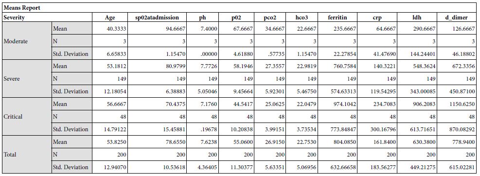
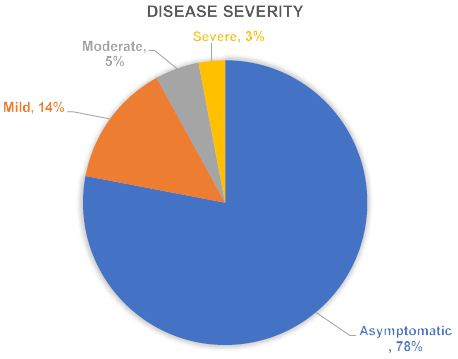
Age range in this study was from 15 to 65 years with mean age of 44.97 ± 10.78 years as shown in Table- I. Out of these 78 patients, 61 (78.21%) were female and 17 (21.79%) were male with female to male ratio of 3.6:1 (Figure I). On the basis of histopathological diagnosis half (39) cases belonged to benign neoplasms and other half (39) were diagnosed as malignant neoplasms as shown in Figure II.

Table 1: Age distribution of patients (n=78), having Mean ± SD = 44.97 ± 10.78 years.

Age (in years)	No. of Patients	%age
15-40	27	34.62
41-65	51	65.38
Total	78	100.0

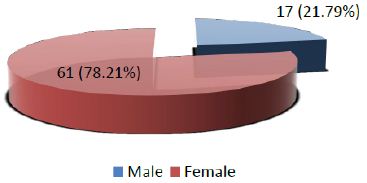
Figure 1: Distribution of patients according to Gender (n=78)

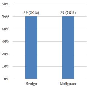
Figure 2: Distribution of patients according to histopathological features (n=78)

Frequency of positive Galectin-3 immunohistochemical expression among thyroid neoplasms was found in 32 out of 78 (41.03%) cases while 46 out of total 78 (58.97%) were showing negative galectin-3 staining (Figure III).

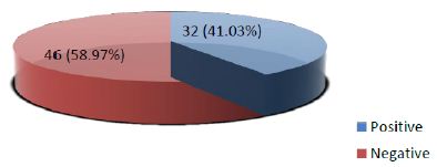
Figure 3: Frequency of Galectin-3 immunohistochemical expression among thyroid neoplasms confirmed on histopathology (n=78)

A detailed look at the further breakdown of galectin-3 staining among benign neoplasms reveal that 11(28.1%) among 39 benign cases were positive for the stain. For the malignant neoplasms, total 21(53.85%) among 39 cases were positive. On the other side 28(71.79%) benign cases and 18(46.15%) malignant cases showed negative galectin-3 staining. The p-value calculated was 0.021 which is not significant (Table- II)

Table 2: Stratification of Galectin-3 immunohistochemical expression among benign and malignant thyroid neoplasms

	Galectin-3 immunohistochemical expression		p-value
	Positive	Negative
Benign	11 (28.21%)	28 (71.79%)	0.021
Malignant	21 (53.85%)	18 (46.15%)

The Stratification of Galectin-3 immunohistochemical expression with respect to age groups showed total 27 cases within the age range of 115- 40 years out of which 10 cases were positive. Total 51 cases belonged to the age range of 41-65 years out of which 22 showed positive galectin-3 staining. The p-value calculated was 0.602 which is again insignificant (Table- III)

Table 3: Stratification of Galectin-3 immunohistochemical expression with respect to age groups

	Galectin-3 immunohistochemical expression		p-value
	Positive	Negative
15-40 years	10	17	0.602
41-65 years	22	29

Similarly Table IV shows the breakdown of the cases according to gender. Total 8 out of 17 cases among male patients were positive for Galectin-3 and 24 out of 61 cases of female patients were showing the positive staining. The p-value calculated was 0.567 which is again insignificant.

Table 4: Stratification of Galectin-3 immunohistochemical expression with respect to gender

	Galectin-3 immunohistochemical expression		p-value
	Positive	Negative
Male	08	09	0.567
Female	24	37

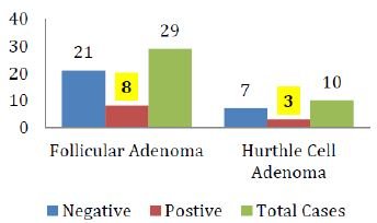
The breakdown of Galectin-3 positivity in the various histological types of malignant and benign thyroid neoplasms is also shown in figure IV & V respectively.

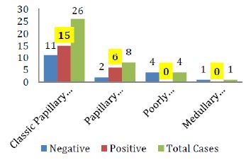
Figure 4: Galectin-3 staining in various histological types of Thyroid carcinomas

Figure 5: Galectin-3 staining in various histological types of Thyroid adenomas

Discussion

Immunohistochemical markers have been extensively investigated for their potential diagnostic and prognostic utility in different thyroid tumors. Among these, they have deduced Galectin-3 to be a promising marker. Galectin-3 belongs to lectin family [9]. And a constellation of other normal tissues and tumors masses express Galectin-3 [10]. An intense nuclear localization of galectin-3 in tumors is seen in malignant transformation of thyroid tissue [11]. Research studies suggest Galectin-3 expression may serve as a potential diagnostic and prognostic marker of some cancers [12]. However, galectin-3 has not been established as a  universal and specific marker of thyroid neoplasia. Yet it can serve as a parameter in diagnostic approach for these tumors and for possible potential therapeutic target [13-16].

In 2015 a study was conducted in India regarding the staining pattern of Galectin-3 in thyroid neoplasms. The results showed 86% sensitivity and 85% specificity, with Galectin-3 showing positive staining in 87% of all malignant and 15% of all benign cases [2] In 2016, another study was conducted in Italy to check the diagnostic accuracy of the various immunohistochemical stains and they found galectin-3 to be 84.2% sensitive and 94.5% specific in detecting the thyroid neoplasms [7].

In contrast, our study shows less frequency of positive Galectin-3 immunohistochemical expression among thyroid neoplasms i.e. total 32 (41.03%) cases with Galectin-3 showing positive staining in 53.85% of all malignant and 28.21% of all benign cases. In 2002 a study was conducted regarding the staining pattern of Galectin-3 in thyroid neoplasms. The results showed high frequency of staining in papillary thyroid carcinomas only and no significant staining in the other type of carcinomas. Moreover, it also showed positive results in follicular adenomas which made them conclude that galectin-3 is not a sensitive marker if used alone [8] Our study also shows the same results.

A systematic review and meta-analysis on galectin-3 as a biomarker found that it may be a potentially useful immuno-marker to distinguish between patients with papillary thyroid carcinoma (PTC) and patients without PTC. In addition, lymph node metastasis is more frequently seen in PTC patients with positive expression of galectin-3 [17]. Our study also gives us the result that although galectin-3 is sensitive for detecting papillary thyroid carcinomas but it is not much sensitive in detecting other carcinomas from benign lesions (adenomas) as shown in figures IV & V.

Galectin-3, HBME-1, and cytokeratin-19 may be helpful in diagnosis of malignant thyroid tumors as evidenced by a study, although the expression of these markers may be seen in benign lesions as well. However, cytokeratin-19 is investigated for its diagnostic prowess. It was found that the marker and its combinations with other markers have higher sensitivities in accurate diagnosis of papillary carcinoma than the other combinations. But these immunohistochemical markers have limited role in differentiation between benign and malignant lesions [18].

Another important point which was noted in this study was that the carcinomas showing positive galectin-3 gave mostly focal positivity rather then the diffuse strong positivity in comparison to the results of the study done by Manivannan et al [18] . That study, which was done in 2012, demonstrated that galectin-3 staining pattern is significant in differentiating benign from malignant follicular neoplasms as well as follicular variant of papillary thyroid carcinoma. Diffuse positivity for galectin-3 was associated with malignant thyroid follicular neoplasms while focal weak positivity favours adenomas. On the other hand, a previous study have demonstrated that there was no marked difference in the staining intensity for intra cytoplasmatic or intranuclear expression of galectin-3 in benign and malignant thyroid neoplasms [19].

Thin-Prep fine needle aspiration cytology  showing increased expression levels of galectin-3 were seen with cellular hyperproliferation, hypertrophy, and pathophysiological situations associated with adenomas and thyroid carcinomas [20-21]. A comparison of glypican-3 (a member of the glypican family of heparan-sulfate proteoglycans bound to the plasma membrane) with galectin-3 demonstrated that galectin-3 had higher sensitivity in diagnosing thyroid carcinoma; however, specificity is low for differentiating follicular-patterned neoplasm [22]. These markers have also been investigated preoperatively and postoperatively, the preoperative serum galectin-3 level showed potential diagnostic value, as it was significantly higher in the cancer patients than in the control subjects (p < 0.05). [23]

Galectin-3 is also used in combination with other biomarkers for a differential diagnosis of thyroid lesions. The most commonly combined biomarkers are Hector Battifora mesothelial epitope-1 (HBME-1) and cytokeratin-19 [24-27]. However galectin-3 may not be used as single discriminators between follicular thyroid adenoma and carcinoma [24-27].  Some studies show that galectin-3 and HBME-1 have an excellent sensitivity and specificity for malignant thyroid lesions (100 and 89.1%, respectively) [26]. Despite core needle biopsies leading to the diagnosis of the majority of thyroid nodules, the accuracy is increased by also observing the galectin-3, cytokeratin-19 and HBME-1 panels, indicating their additional diagnostic value when combined with routine histology and not when used alone [24-27].  It was also reported that galectin 3, cluster of differentiation (CD) and, to an extent, HBME-1, are useful immunocytochemical parameters with the potential to support the fine needle aspiration cytology diagnosis of PTC, particularly in situations where the differential diagnoses is complicated [28].

Studies have noted variable Galectin-3 expression in poorly differentiated thyroid cancers also [29]. However, in majority of cases (75% to 100% of reported cases) of anaplastic thyroid carcinoma, Galectin-3 positivity was identified suggesting that differentiated thyroid carcinoma can progress or undergo anaplastic transformation [26,29]. In the present study and study by Herrmann et al., small number of cases of MTC and poorly differentiated carcinoma are reported with inconsistent Galectin-3 expression, making diagnostic application of Galectin-3 in these rare histological subgroups unlikely [30].

Zhu et al. reported several markers expression like HBME-1, CK-19, Galectin-3, and RET in several papillary thyroid carcinoma. The expression was found to be higher in papillary thyroid carcinoma as compared to benign neoplasia. However, they did not report any of these as specific markers for papillary thyroid carcinoma [31].

Conclusion

Galectin-3 immunohistochemical expression is found in the cases of both benign thyroid tumors and malignant neoplasms although more  commonly seen in malignant ones. So, it cannot be used alone for the routine diagnosis of malignant thyroid lesions as it shows less sensitivity and specificity. It also has expressed limited role in differentiating between the benign and the malignant thyroid neoplasms.

References

1. Braverman LE, Cooper D. (2012) Werner & Ingbar’s The Thyroid: A Fundamental and Clinical Text. 10^th Philadelphia: Lippincott Williams & Wilkins. p. 10.
2. Sumana BS, ShaShidhar S, Shivarudrappa AS, (2015) Galectin-3 Immunohistochemical Expression in Thyroid Neoplasms. Journal of Clinical and Diagnostic Research 9:EC07. [crossref]
3. Pellegriti G, Frasca F, Regalbuto C, Squatrito S, Vigneri R. (2013) Worldwide Increasing Incidence of Thyroid Cancer: Update on Epidemiology and Risk Factors. Journal of Cancer Epidemiology. [crossref]
4. Dwivedi SS, Khandeparkar SG, Joshi AR, Kulkarni MM, Bhayekar P, Jadhav A, et al. (2016) Study of Immunohistochemical Markers (CK-19, CD-56, Ki-67, p53) in Differentiating Benign and Malignant Solitary Thyroid Nodules with Special Reference to Papillary Thyroid Carcinomas. Journal of Clinical and Diagnostic Research 10:EC14-9. [crossref]
5. Asif F, Ahmad MR, Majid A. (2015) Risk Factors for Thyroid Cancer in Females Using a Logit Model in Lahore, Pakistan. Asian Pacific Journal of Cancer Prevention 16:6243-7. [crossref]
6. Fortuna-Costa A, Gomes AM, Kozlowski EO, Stelling MP, Pavão MS. (2014) Extracellular Galectin-3 in Tumor Progression and Metastasis. FrontOncol 4:138. [crossref]
7. Trimboli P, Guidobaldi L, Amendola S, Nasrollah N, Romanelli F, Attanasio D, et al. (2016) Galectin-3 and HBME-1 Improve the Accuracy of Core Biopsy in Indeterminate Thyroid Nodules. Endocrine 52:39-45. [crossref]
8. Fukumori T, Kanayama H, Raz A. (2007) The Role of Galectin-3 in Cancer Drug Resistance. Drug Resistance Updates 10:101-8. [crossref]
9. Hirabayashi J, Kasai K. (1993) The Family of Metazoan Metal-Independent Beta-Galactoside-Binding Lectins: Structure, Function and Molecular Evolution. Glycobiology 3:297-304. [crossref]
10. Dumic J, Dabelic S, Flogel M. (2006) Galectin-3: An Open-Ended Story. Biochimica et Biophysica Acta 1760:616-35. [crossref]
11. Paron I, Scaloni A, Pines A, Bachi A, Liu FT, Puppin C, Pandolfi M, Ledda L, Di Loreto C, Damante G et al. (2003) Nuclear Localization of Galectin-3 in Transformed Thyroid Cells: A Role in Transcriptional Regulation. Biochemical and Biophysical Research Communications 302:545-53.
12. Danguy A, Camby I, Kiss R. (2002) Galectins and Cancer. Biochimica et Biophysica Acta 1572:285-93. [crossref]
13. Van den Brule F, Califice S, Castronovo V. (2004) Expression of Galectins in Cancer: A Critical Review. Glycoconjugate Journal 19:537-42. [crossref]
14. Johnson KD, Glinskii OV, Mossine VV, Turk JR, Mawhinney TP, Anthony DC, et al. (2007) Galectin-3 As a Potential Therapeutic Target in Tumors Arising from Malignant Endothelia. Neoplasia 9:662- 70. [crossref]
15. Sawangareetrakul P, Srisomsap C, Chokchaichamnankit D, Svasti J. (2008) Galectin-3 Expression in Human Papillary Thyroid Carcinoma. Cancer Genomics & Proteomics 5:117- 22. [crossref]
16. Nangia-Makker P, Nakahara S, Hogan V, Raz A. (2007) Galectin-3 in Apoptosis, a Novel Therapeutic Target. Journal of Bioenergetics and Biomembranes 1:79- 84.
17. Tang W, Huang C, Tang C, Xu J, Wang H. (2016) Galectin-3 may serve as a Potential Marker for Diagnosis and Prognosis in Papillary Thyroid Carcinoma: A Meta-Analysis. OncoTargets and Therapy 9:455–60. [crossref]
18. Manivannan P, Siddaraju N, Jatiya L, Verma SK. (2012) Role of Pro-Angiogenic Marker Galectin-3 in Follicular Neoplasms of Thyroid. Indian Journal of Biochemistry and Biophysics 49:392–4. [crossref]
19. Sumana BS, Shashidhar S, Shivarudrappa AS. (2015) Galectin-3 Immunohistochemical Expression in Thyroid Neoplasms. Journal of Clinical and Diagnostic Research 9:EC07–11. [crossref]
20. Papale F, Cafiero G, Grimaldi A, Marino G, Rosso F, Mian C, Barollo S, Pennelli G, Sorrenti S, De Antoni E, Barbarisi A. (2013) Galectin-3 Expression in Thyroid Fine Needle Cytology (t-FNAC) Uncertain Cases: Validation of Molecular Markers and Technology Innovation. Journal of Cellular Physiology 228:968–74. [crossref]
21. Salajegheh A, Dolan-Evans E, Sullivan E, Irani S, Rahman MA, Vosgha H, Gopalan V, Smith RA, Lam AK. (2014) The Expression Profiles of the Galectin Gene Family in Primary and Metastatic Papillary Thyroid Carcinoma with Particular Emphasis on Galectin-1 and Galectin-3 Expression. Experimental and Molecular Pathology 96:212–8. [crossref]
22. Al-Sharaky DR, Younes SF. (2016) Sensitivity and Specificity of Galectin-3 and Glypican-3 in Follicular-Patterned and other Thyroid Neoplasms. Journal of Clinical and Diagnostic Research 10:EC06–10. [crossref]
23. Yilmaz E, Karsidag T, Tatar C, Tüzün S. (2015) Serum Galectin-3: Diagnostic Value for Papillary Thyroid Carcinoma. Ulus Cerrahi Derg 31:192–6. [crossref]
24. Paunovic I, Isic T, Havelka M, Tatic S, Cvejic D, Savin S. (2012) Combined Immunohistochemistry for Thyroid Peroxidase, Galectin-3, CK19 and HBME-1 in Differential Diagnosis of Thyroid Tumors. APMIS 120:368–79. [crossref]
25. Abd-El Raouf SM, Ibrahim TR. (2014) Immunohistochemical Expression of HBME-1 and Galectin-3 in the Differential Diagnosis of Follicular-Derived Thyroid Nodules. Pathology, Research and Practice 210:971–8. [crossref]
26. Trimboli P, Guidobaldi L, Amendola S, Nasrollah N, Romanelli F, Attanasio D, et al. (2016) Galectin-3 and HBME-1 Improve the Accuracy of Core Biopsy in Indeterminate Thyroid Nodules. Endocrine 52:39–45.
27. Durry MF, Miskad UA, Leiwakabessy WN, Cangara MH. (2016) Diagnostic Value of Galectin-3 and Hector Battifora Mesothelial Epitope (HBME)-1 as a Marker for Malignancy in the Diagnosis of Thyroid Lesions. Pathology International 48:S122–3.
28. Das DK, Al-Waheeb SK, George SS, Haji BI, Mallik MK. (2014) Contribution of Immunocytochemical Stainings for galectin-3, CD44, and HBME1 to Fine-Needle Aspiration Cytology Diagnosis of Papillary Thyroid Carcinoma. Diagn Cytopathol 42:498–505.
29. Bartolazzi A, Gasbarri A, Papotti M, Bussolati G, Lucante T, Khan A, et al. (2001) Application of an Immunodiagnostic Method for Improving Preoperative Diagnosis of Nodular Thyroid Lesions. Lancet 357:1644–50. [crossref]
30. Herrmann ME, LiVolsi VA, Pasha TL, Roberts SA, Wojcik EM, Baloch ZW. (2002) Immunohistochemical Expression of Galectin-3 in Benign And Malignant Thyroid Lesions. Archives of Pathology & Laboratory Medicine 126:710–13. [crossref]
31. Zhu X, Sun T, Lu H, Zhou X, Lu Y, Cai X, Zhu X. (2010) Diagnostic Significance of CK19, RET, galectin-3 and HBME-1 Expression for Papillary Thyroid Carcinoma. Journal of Clinical Pathology 63:786-9. [crossref]

DOI: 10.31038/EDMJ.2021531

Abstract

Introduction: Covid-19 disease is a global pandemic caused by severe acute respiratory syndrome coronavirus 2 (SARS‑CoV‑2). Researchers all over the world are trying their best to identify its causative factors, patho- physiology and treatment modalities. Retrospective cohort studies carried out in China showed significant mortality and morbidity associated with high D dimers value in admitted patients. We aimed to see the association of D dimers with the prognosis of covid-19.

Methods: This Retrospective Cross-sectional study was done at Benazir Bhutto hospital Rawalpindi during May –June 2020 obtaining a sample of 200 patients. All those patients being admitted in COVID ward were assessed on the basis of D dimers and their 28 day outcome. Ethical approval was solicited from the Institutional Research Forum of Rawalpindi Medical University.

Results: The study yielded 200 participants in which the patients with moderate severity of the disease had a mean age of 40.33±6.65, that with severe disease had a mean age of 53.18±12.1 and critical patients had a mean age of 56.67±14.79. The disease severity is significantly related to increased mean age of the patient (p = 0.050). Mean serum ferritin levels in patients with moderate disease was 235.67±22.27 micrograms per liter, the patients with severe disease had mean value of 760.75±574.63 micrograms per liter and critical patients had a mean ferritin level of 974.10±773.85 micrograms per liter. This revealed that the ferritin levels increased significantly in patients with severe disease

Conclusion: Our findings establish a consistent increase in the levels of D-dimers with increasing severity of the disease, from mild to severe to critical patients. D –Dimers are important predictors of prognosis and disease severity which can be utilized to evaluate the treatment outcomes in COVID-19 infection. Further studies are recommended to find out the cut-off value of D-dimers as a biomarker of disease severity.

Introduction

Covid-19 disease is a global pandemic caused by severe acute respiratory syndrome coronavirus 2 (SARS‑CoV‑2) [1]. It was initially identified in city of Wuhan in December 2019 [2]. World Health Organization declared corona virus as a pandemic on 11 March 2020 [3]. It is a virus of zoonotic origin thought to be transmitted by air borne route. Symptoms of COVID-19 can be relatively non-specific; most common symptoms are fever, dry cough ,sore throat ,shortness of breath, myalgias, abdominal pain ,diarrhea, loss of sense of smell and taste  [4]. Approximately one in five patients who become symptomatic become critical and suffer breathing difficulties, persistent chest pain, sudden confusion, difficulty waking, and bluish face or lips. Complications include pneumonia, acute respiratory distress syndrome, sepsis, septic shock, and kidney failure [5]. Covid-19 related complications are associated with high mortality rate.

Researchers all over the world are trying their best to identify its causative factors, patho- physiology and treatment modalities. Retrospective cohort studies carried out in China showed significant mortality and morbidity associated with high D dimers value in admitted patients [6]. COVID related  Acute Respiratory Distress Syndrome (ARDS) showed a pro coagulant pattern and this state depicted significant mortality with pulmonary embolism. Covid-19 infection triggered a inflammatory cytokine response which initiated a thrombotic state .It was observed in many studies mortality was reduced by anticoagulation with Low Molecular Weight Heparin (LMWH). The coagulation abnormalities seen in COVID are different from that seen in DIC (sepsis). In DIC, thrombocytopenia is a key finding along with elevated clotting time. However, in cohorts non-surviving patients had an average platelet count and a pro thrombin time which falls within the normal range. It thus may be more likely that local rather than disseminated thrombin generation is at play in COVID-19 patients [7-9].

The main aim of our study was to see the association of D dimers with the prognosis of covid-19. Our study investigated COVID patients and role of D dimers in their mortality and morbidity. There is lack of international & local studies, therefore our study will have a huge impact on researchers and the national data base.

Material & Methods

This Retrospective Cross-sectional study was done at Benazir Bhutto hospital Rawalpindi, which was nominated by Punjab government as COVID Dedicated Unit. Sampling technique used was consecutive sampling. Total sample size obtained was 200 patients. All those patients being admitted in COVID wards during 2 months May- June 2020 were assessed on the basis of D dimers and their 28 day outcome. As d dimers is an easy and inexpensive test was used a screening tool for risk stratification of Covid-19 patients.

Cases of corona virus infection were confirmed by RT-PCR. A patient diagnosed as COVID-19 on the basis of ABI 7500 Real Time RT-PCR detection system after RNA extraction (Qiagen Viral RNA Mini Kit) with internal and external positive controls, using the SARS-CoV-2 protocol.

Inclusion & Exclusion Criteria

Confirmed COVID-19 cases were included in our study where as pregnant women, patients having any hematologic malignancy, chronic liver disease, acute coronary syndrome, surgery or trauma within 30 days and patients without D-dimer testing upon admission were excluded from our study.

Data Collection Technique

Demographic, clinical lab data and outcome (survival or death) was collected form patient records and recorded on self-designed proforma. Disease Severity was be defined as per WHO criteria into moderate, severe, critical with ARDS and Critical with Sepsis/Septic shock. Patients were grouped into two : group A (D-dimer < 500ng/ml) and Group B ( D-dimer ≥ 500ng/ml).

Data Analysis

Data was analyzed via SPSSv25.0. Numerical data was represented as mean and standard deviation. Independent sample t test was used to compare difference of means of numerical variables across severity of the disease according to WHO criteria. Categorical variables were represented as frequencies (%). Distribution of frequencies across severity was compared by Chi-Square test. ROC curve was plotted to determine the cut-off point for D-Dimer to predict mortality.

Ethical Consideration

Ethical approval was solicited from the Institutional Research Forum of Rawalpindi Medical University before securing access to patient data.

Results

The study yielded 200 participants with a mean age of 53.82±12.94 years. On the basis of stratification of severity, the patients with moderate severity of the disease had a mean age of 40.33±6.65, that with severe disease had a mean age of 53.18±12.1 and critical patients had a mean age of 56.67±14.79. The disease severity is significantly related to increased mean age of the patient (p = 0.050). At the time of admission, the patients with moderate disease had a mean SpO₂ of 94.67±1.15%, patients with severe disease had a mean SpO₂ of 80.79±6.39%, and critical patients had a mean SpO₂ of 70.43±15.46%. The mean oxygen saturation at the time of admission decreased with increasing severity (p = 0.000). The patients with moderate disease had a mean arterial partial pressure of oxygen (pO₂) of 66.67±6.61 mmHg, patients with severe disease had a mean pO₂ of 58.19±9.45 mmHg, and critical patients had a mean pO₂ of 44.54±10.21 mmHg. The mean partial pressure of oxygen showed a decline with increasing severity (p = 0.000). Regarding mean arterial partial pressure of carbon dioxide in the patients, the patients with moderate disease had pCO₂ of 34.67±6.61 mmHg, patients with severe disease had a mean pCO₂ of 27.35±5.92 mmHg, and critical patients had a mean pCO₂ of 25.06±3.99 mmHg. The mean partial pressure of carbon dioxide showed a decline with increasing severity (p = 0.002). Mean serum ferritin levels in patients with moderate disease was 235.67±22.27 micrograms per liter, the patients with severe disease had mean value of 760.75±574.63 micrograms per liter and critical patients had a mean ferritin level of 974.10±773.85 micrograms per liter. This revealed that the ferritin levels increased significantly in patients with severe disease. Upon investigating the levels of C-Reactive protein, mean serum CRP levels in patients with moderate disease was 235.67±22.27 mg/L, the patients with severe disease had mean value of 760.75±574.63 mg/L and critical patients had a mean ferritin level of 974.10±773.85 mg/L.

Discussion

Laboratory Hemostasis is believed to provide a very strong evidence in screening, definitive diagnosis and prognosis of many human pathologies [10]. Measuring the levels of D-dimers is one of them. D-dimers are the products of fibrin degradation, which serve as a biomarker in a lot of diseases associated with coagulopathies e.g in coronary artery atherosclerosis, Disseminated intravascular disease and Venous Thromboembolism [11]. D-dimer levels have played a significant role in the evaluation of patients suffering from Community Acquired Pneumonia [12], 2009 novel influenza A (H1N1) [13] and various other members of Coronaviridae family. Covid-19 has also been associated with an increased risk of Venous Thromboembolism [14-15-16]. Hence, the coagulopathy involved in Covid-19 infections can serve as a major determinant of disease prognosis [17]. The levels of D-dimers are consistently elevated in patients suffering from Covid-19 [18-19-20]. In this study, we aimed to explore the association of D-dimer levels with disease severity of Covid-19.

Our findings establish a consistent increase in the levels of D-dimers with increasing severity of the disease, from mild to severe to critical patients [Table 1]. The severity of these patients depended on the duration for which these patients remained in the hospital under care. A strong association was established between these two (Eta sq. 0.128). Many studies concluded the increasing levels of D-dimers to be associated with severity of Covid patients. Huang et al. studies the data of 41 patients and reported a five-fold increase in critical patients  (median: 2.4 mg/L; IQR: 0.6–14.4 mg/L) as compared to the non-critical ones (median: 0.5 mg/L; IQR: 0.3–0.8 mg/L; p  = 0.004) [21]. Another study was performed by Zhou et al. (16). He reported a nine-fold increase in patients who died of Covid (median: 5.2 mg/L; IQR: 1.5–21.1 mg/L) than in those who survived (median: 0.6 mg/L; IQR: 0.3–1.0 mg/L; p  < 0.001). Tand et al. [22] and Wang et al. [23] also had consistent findings as ours. Moreover, irrespective of age, BMI, sex, Hypertension or Diabetes, increased coagulation biomarkers in Covid patients invariably required an increased Oxygen supply, which again can be linked as increased severity in patients having adverse coagulopathies [24].

Table 1: Showing study variables and their severity along with p value.

Study variables		Number (n)	Percentage (%)	Severity				p-value
Gender
	Male	126	63	1	96	29	126	0.496
	Female	74	37	2	53	19	74
Shortness of Breath
	Yes	179	89.5	2	134	43	179	0.429
	No	21	10.5	1	15	5	21
Fever
	Yes	100	50.0	1	77	22	100	0.659
	No	100	50.0	2	72	26	100
Cough
	Yes	46	23.0	1	77	22	100	0.494
	No	154	77.0	2	72	26	100
Sore Throat
	Yes	19	9.5	0	17	2	19	0.282
	No	181	90.5	3	132	46	181
Diarrhea
	Yes	11	5.5	1	6	4	11	0.057
	No	187	93.5	2	141	44	187
Diabetes Mellitus
	Yes	94	47.0	2	62	30	94	0.033
	No	106	53.0	1	87	18	106
Hypertension
	Yes	94	47.0	0	73	21	94	0.212
	No	106	53.0	3	76	27	106
Ischemic Heart Disease
	Yes	37	18.5	0	27	10	37	0.648
	No	163	81.5	3	122	38	163
Chronic Obstructive Pulmonary Disease
	Yes	9	4.5	0	6	3	9	0.755
	No	191	95.5	3	143	45	191
Asthma
	Yes	11	5.5	0	9	2	11	0.810
	No	189	94.5	3	140	46	189
Rheumatoid Arthritis
	Yes	3	1.5	0	3	0	3	0.594
	No	197	98.5	3	146	48	197
Chronic Kidney Disease
	Yes	7	3.5	0	5	2	7	0.914
	No	193	96.5	3	144	46	193
Hepatitis B/C Infection
	Yes	7	3.5	0	6	1	7	0.773
	No	193	96.5	3	143	47	193
Hypothyroidism
	Yes	7	3.5	0	5	2	7	0.913
	No	193	96.5	3	144	46	193
PCR
	Positive	152	76.0	3	108	41	152	0.117
	Negative	48	24.0	0	41	7	48
Arterial Blood Gases (ABG) Interpretation
	Normal	68	34.0
	Acute respiratory Failure 1	126	63.0
	Acute respiratory Failure 2	2	1.0
	Compensated/Chronic Respiratory Failure	4	2.0
Oxygen Flow
	Normal	110	55.0
	High Flow	60	30.0
	Low Flow	30	15.0
Oxygen Support Device
	NRBM	108	54.0
	Nasal canula	3	1.5
	BIPAP	8	4.0
	Face Mask	42	21.0
	Ventilator	30	15.0
	None	8	4.0
Methylprednisolone Therapy
	Yes	101	50.5	2	73	26	101	0.702
	No	99	49.5	1	76	22	99
Dexamethasone Therapy
	Yes	156	78.0	2	73	26	101	0.151
	No	44	22.0	1	76	22	99
Ivermectin Therapy
	Yes	117	58.5	3	98	16	117	0.000
	No	83	41.5	0	51	32	83
Tocilizumab Therapy
	Yes	25	12.5	0	20	5	25	0.692
	No	175	87.5	3	129	43	175
Heparin Therapy
	Yes	177	88.5	3	134	40	177	0.377
			11.5	0	15	8	23
Outcome
	Expired	36	18.0	0	0	36	36	0.000
	Improved	160	80.0	3	148	9	160
	Critical	4	2.0	0	1	3	4
Severity
	Moderate	3	1.5
	Severe	149	74.5
	Critical	48	24.0

The underlying biological plausibility and pathogenesis behind increased D-dimers in Covid-19 can be understood by the disease triggering an inflammatory response. Covid-19 is associated with increased acute phase reactant proteins e.g CRP, as shown in [Table 2] of our findings. Other studies also show a consistent increase in CRP levels with an associated mortality rate of 30 days in coronavirus patients [25]. In the consequence of inflammation, proinflammatory cytokines such as Interleukin 1 (IL-1), Interleukin 6 (IL-6) and tumor necrosis factor-α (TNF-α) are elevated [20]. This results in a cytokine storm that triggers monocytes and macrophages to express tissue factor which leads to thrombin generation [26]. There is also an endothelial damage which results in increased plasma concentrations of tissue-type plasminogen activator (t-PA), upto six-fold increase [27]. This explains the increased levels of D-dimers in Covid-19 patients. Moreover, an accompanied increase in metalloproteinases explains the extracellular matrix modification, resulting in capillary damage and pulmonary edema. The remarkable fibrinolytic profile of Covid patients has also been explained by the studies performed in mice [28]. However, it is noteworthy that increased fibrinolytic profile can still not be translated as DIC or hyper fibrinolytic state. Although coagulopathy may reflect some similar findings, but Covid coagulopathy has a very complex etiology, resulting from intricate interactions between the immune system and coagulation system in the host [29].

Table 2: Showing underlying biological plausibility and pathogenesis behind increased D-dimers in Covid-19.

The ROC curve of our findings for the D-dimer test with severity of Covid diseases is shown in [Figure 1]. The area under the curve (AUC) is 0.699.  It can be utilised to determine a definitive cut-off value to support the International Society of Thrombosis and Haemostasis (ISTH) arbitrary definition of raised D-dimers in coronavirus patients as done by Zhang et al [30].

Figure 1: ROC for D-Dimer as a Predictor of Outcome in COVID-19 Infection Area Under the Curve (AUC) is 0.669

Limitations

There are a few limitations in our study that need to be known. Firstly, the burden of the pandemic itself and an emergency situation in Pakistan has hindered the practicality of Cohort, Case-control or Randomized Control Trial- which could have provided a greater pool of Clinical and Lab findings; making even better associations possible. Secondly, we cannot exclude the strong association of confounding factors with coagulopathies- hence a stratified analysis of these confounders can give us a better picture of using D-dimers as a prognostic marker in Covid-19 patients. Moreover, limitations in the measurement of plasma D-dimer concentration may also exist at the level of Laboratory methods and skills involved at human level [31].

Conclusion

COVID-19 infection is characterized by hypercoagulability, inflammation, and multi-organ damage mediated by cytokines. These pathologies are manifested by appearance of several acute phase proteins and inflammatory markers in the serum. The levels of these biomarkers are variable in various stages of COVID-19 infection in relation to severity. The prognosis can be predicted by these serum biomarkers. In this study, D-dimers are measured in patients at various stages of disease severity. D-dimers are important predictors of prognosis and disease severity. These biomarkers can be utilized to evaluate the treatment outcomes in COVID-19 infection. Further studies are recommended to find out the cut-off value of D-dimers as a biomarker of disease severity.

Conflict of Intrest

Nill to disclose

Funding

Nill to disclose

References

1. Zu ZY, Jiang MD, Xu PP, et al. (2020) Coronavirus Disease 2019 (COVID-19): A Perspective from China. Radiology Aug;296(2):E15-E25. doi: 10.1148/radiol.2020200490. Epub 2020 Feb 21. [crossref]
2. Sahin AR, Erdogan A, Agaoglu PM, et al. (2020) 2019 novel coronavirus (COVID-19) outbreak: a re-view of the current literature. EJMO 4(1):1_7.
3. https://www.who.int/news/item/23-01-2020-statement-on-the-meeting-of-the-international-health-regulations-(2005)-emergency-committee-regarding-the-outbreak-of-novel-coronavirus-(2019-ncov)
4. Hopkins C. “Loss of sense of smell as marker of COVID-19 infection”. Ear, Nose and Throat surgery body of United Kingdom. Retrieved 28 March 2020.
5. Interim Clinical Guidance for Management of Patients with Confirmed Coronavirus Disease (COVID-19)”. S. Centers for Disease Control and Prevention (CDC) Retrieved 11 April 2020. https://www.cdc.gov/coronavirus/2019-ncov/hcp/clinical-guidance-management-patients.html.
6. Lippi G, Favaloro EJ (2020) D-dimer is Associated with Severity of Coronavirus Disease 2019: A Pooled Analysis. Thromb Haemost May;120(5):876-878. doi: 10.1055/s-0040-1709650. Epub 2020 Apr 3. [crossref]
7. Tang N, Li D, Wang X, et al. (2020) Abnormal coagulation parameters are associated with poor prognosis in patients with novel coronavirus pneumonia. J Thromb Haemost Apr;18(4):844-847. doi: 10.1111/jth.14768. Epub 2020 Mar 13. [crossref]
8. Ranucci M, Ballotta A, Di Dedda U, et al. (Jul. 2020) The procoagulant pattern of patients with COVID-19 acute respiratory distress syndrome. J Thromb Haemost 18(7):1747-1751. doi: 10.1111/jth.14854. Epub 2020 May 6. [crossref]
9. Wang T, Chen R, Liu C, et al. (May 2020) Attention should be paid to venous thromboembolism prophylaxis in the management of COVID-19. Lancet Haematol 7(5):e362-e363. doi: 10.1016/S2352-3026(20)30109-5. Epub 2020 Apr 9. [crossref]
10. Lippi G, Favaloro EJ (Jun. 2018) Laboratory hemostasis: from biology to the bench. Clin Chem Lab Med 27;56(7):1035-1045. doi: 10.1515/cclm-2017-1205.  [crossref]
11. Soomro AY, Guerchicoff A, Nichols DJ, et al. (Jul. 2016) The current role and future prospects of D-dimer biomarker. Eur Heart J Cardiovasc Pharmacother 2(3):175-84. doi: 10.1093/ehjcvp/pvv039. Epub 2015 Sep 27. [crossref]
12. Chalmers J.D., Singanayagam A., Scally C., et al. (2009) Admission D-dimer can identify low-risk patients with community-acquired pneumonia. Emerg. Med. 53:633–638. doi: 10.1016/j.annemergmed.2008.12.022. [crossref]
13. Wang Z.F., Su F., Lin X.J., et al. (2011) Serum D-dimer changes and prognostic implication in 2009 novel influenza A(H1N1). Res 127:198–201. doi: 10.1016/j.thromres.2010.11.032. [crossref]
14. Helms J., Tacquard C., Severac F., et al. (2020) High risk of thrombosis in patients with severe SARS-CoV-2 infection: A multicenter prospective cohort study. Intensive Care Med 46:1089–1098. doi: 10.1007/s00134-020-06062-x. [crossref]
15. Leonard-Lorant I., Delabranche X., Severac F, et al. Acute Pulmonary Embolism in COVID-19 Patients on CT Angiography and Relationship to D-Dimer Levels. Radiology. 2020:201561. doi: 10.1148/radiol.2020201561. [crossref]
16. Fauvel C., Weizman O., Trimaille A., et al. (2020) Pulmonary embolism in COVID-19 patients: A French multicentre cohort study. Heart J. 41:3058–3068. doi: 10.1093/eurheartj/ehaa500. [crossref]
17. Tang N., Li D., Wang X., et al. (2020) Abnormal coagulation parameters are associated with poor prognosis in patients with novel coronavirus pneumonia. Thromb. Haemost. 18:844–847. doi: 10.1111/jth.14768. [crossref]
18. Thachil J (2020) All those D-dimers in COVID-19. Thromb. Haemost. doi: 10.1111/jth.14939. [crossref]
19. Lippi G. (2020) Favaloro E.J. D-dimer is Associated with Severity of Coronavirus Disease 2019: A Pooled Analysis. Haemost. 120:876–878. doi: 10.1055/s-0040-1709650. [crossref]
20. Huang C, Wang Y, Li X et al. (2020) Clinical features of patients infected with 2019 novel coronavirus in Wuhan, China. Lancet 395(10223):497–506. [crossref]
21. Zhou F, Yu T, Du R et al. (2020) Clinical course and risk factors for mortality of adult inpatients with COVID-19 in Wuhan, China: a retrospective cohort study. Lancet S0140-6736(20)30566-3. [crossref]
22. Tang N, Li D, Wang X, et al. (2020) Abnormal coagulation parameters are associated with poor prognosis in patients with novel coronavirus pneumonia. J Thromb Haemost Doi: 10.1111/jth.14768. [crossref]
23. Wang D, Hu B, Hu C, et al. (2020) Clinical characteristics of 138 hospitalized patients with 2019 novel coronavirus-infected pneumonia in Wuhan, China. JAMA Doi: 10.1001/jama.2020.1585. [crossref]
24. https://onlinelibrary.wiley.com/doi/10.1111/jth.15067
25. Huang I, Pranata R, Lim MA, et al. (Jan.-Dec. 2020) C-reactive protein, procalcitonin, D-dimer, and ferritin in severe coronavirus disease-2019: a meta-analysis. Ther Adv Respir Dis 14:1753466620937175. doi: 10.1177/1753466620937175. [crossref]
26. Levi M, Thachil J. (2020) Coronavirus disease 2019 coagulopathy: disseminated intravascular coagulation and thrombotic microangiopathy-either, neither, or both. Semin Thromb Hemost 46:781–784. doi: 10.1055/s-0040-1712156. [crossref]
27. Liu ZH, Wei R, Wu YP, et al. (2005) Elevated plasma tissue-type plasminogen activator (t-PA) and soluble thrombomodulin in patients suffering from severe acute respiratory syndrome (SARS) as a possible index for prognosis and treatment strategy. Biomed Environ Sci BES 18:260–264. [crossref]
28. Gralinski LE, Bankhead A, Jeng S, et al. (2013) Mechanisms of severe acute respiratory syndrome coronavirus-induced acute lung injury. mBio 4:e00271–e313. doi: 10.1128/mBio.00271-13. [crossref]
29. Iba T, Levy JH, Levi M, et al. (Sep. 2020) Coagulopathy of Coronavirus Disease 2019. Crit Care Med 48(9):1358-1364. doi: 10.1097/CCM.0000000000004458. [crossref]
30. Zhang L et al. (2020) D-dimer levels on admission to predict in-hospital mortality in patients with Covid-19. Journal of Thrombosis and Haemostasis 18, 1324–1329. [crossref]
31. Hardy M., Lecompte T., Douxfils J, et al. (2020) Management of the thrombotic risk associated with COVID-19: Guidance for the hemostasis laboratory. J. 18:17. doi: 10.1186/s12959-020-00230-1. [crossref]

DOI: 10.31038/EDMJ.2021533

Abstract

Introduction: Coronavirus disease of 2019 started started in Wuhan China as an epidemic causing pneumonia-like illness. It became a global pandemic in a period of two months. On January 30, 2020, the World Health Organization (WHO) declared the outbreak of COVID-19 as the sixth global public health emergency (PHEIC), and on March 11, 2020, the WHO declared COVID-19 a pandemic. The waves in the epidemiological curve of the pandemic show the the progression of the pandemic. Our study aims at evaluating the the patient characteristics in first and second curve of COVID-19 pandemic.

Materials and Methods: We conducted a prospective study of all hospitalized cases of SARS COV-2 infection in KRL Hospital Islamabad, admitted between March 2020 and February 2021. All patients admitted upto August 2020 were considered in 1st wave & all those admitted from September 2020 to February 2021 were considered in 2nd wave which divided the study groups into two equal parts i.e., 6 months.

Results: In this study, the average length of stay in both waves was similar (10 days). The second wave of the pandemic inflicted younger patients greater than the first wave of the pandemic. The difference of severity of disease in the patient presenting in the first and second waves was insignificant (p > 0.05).

Conclusion: COVID-19 cases presented differently in both first and second waves of COVID-19 pandemic. The comparison of case presentation and severity of disease may help the healthcare professionals and epidemiologists to valuate the treatment and management methods. It may highlight the effectiveness of administrative aspects of controlling the pandemic.

Introduction

Coronavirus-19 (COVID-19), produced by the acute respiratory tract coronavirus 2 (SARS-CoV-2), has become a global epidemic, posing a serious health threat worldwide. Several countries have seen the pattern of two reported cases, the first wave in spring and the second in late summer and autumn [1-3]. On January 30, 2020, the World Health Organization (WHO) declared the outbreak of COVID-19 as the sixth global public health emergency (PHEIC), and on March 11, 2020, the WHO declared COVID-19 a pandemic [4]. The first case of COVID-19 was reported from Karachi on February 26, 2020, when the estimated population of Pakistan was 204.65.3,4 million [5]. As a result of the outbreak, the government introduced a series of rigorous prevention measures, including home confinement, followed by a three-month period of increased social networking, performance and hard work. With social life in the country it was back to normal, without the obligation to wear a mask and keep the public space safe. Unfortunately, the number of patients with COVID-19 began to skyrocket in August and a month later it showed the same numbers as in April. This has forced the government to reinstate drastic measures to prevent, including the closure of facilities and facilities, the closure of parks, restaurants, cultural and sports activities, and the curfew. The number of cases in Pakistan has continued to grow since then, sometimes downwards, and at the time of writing this article seems to be declining slightly. The second wave of COVID-19 was predicted months ago and already existed in some countries [6]. After the relaxation of the measures in the summer, the second wave began in mid-September 2020 and expanded until March 2021 [7]. While some countries have a second wave that is much better than the first. Meanwhile more than 20,000 people have died compared to less than 10,000 across the first wave, which is a clear indication that the medical services at hospitals were second only around [8].

This study investigated the severity and characteristics of the two waves in hospitalized patients in Islamabad.

Material & Methods

We conducted a prospective study of all hospitalized cases of SARS COV-2 infection in KRL Hospital Islamabad, admitted between March 2020 and February 2021.

All patients admitted unto August 2020 were considered in 1^st wave & all those admitted from September 2020 to February 2021 were considered in 2^nd wave, which divided the study groups into two equal parts i.e. 6 months.

All the patients who were hospitalized with diagnosis of SARS-COV-2 (Covid Pneumonia) were included in the study. Those with suspected SARS-COV-2 infection but no laboratory confirmation were excluded from the study. SARS-COV-2  infection was confirmed using RT-PCR using swab samples from upper respiratory tract  (nasopharyngeal / oropharyngeal swabs).

The Ethical Review Board, KRL Hospital Islamabad, approved this study.

Results

Figure 1: (1^st wave) showing month wise data of all COVID-19 PCR tests conducted and positivity rate for COVID-19 infection. 57027 tests performed till 30th September 2020. COVID-19 PCR positivity rate was 2.1% which equal to national positivity rate.

Figure 2: (1^st wave)The average length of stay was 10 days with high recovery rate at 99%.

Figure 3: (1^st wave) Asymptomatic: With no symptoms, only PCR positive. Mild Symptoms: Fever (1000F – 1020F) shortness of breath on exertion, body aches, maintaining>95% oxygen saturation at room air. Moderate: Fever (1010F – 1030F) shortness of breath, myalgia’s, oxygen saturation at 3-5 liters max with NIV nasal cannula. Sever Disease illness: Fever (1010F – 1030F) shortness of breath, body aches, myalgia, prominent changes on imaging and difficulty in maintaining blood oxygen saturation with NIV nasal cannula (highly oxygen dependent).

Figure 4: Second Wave showing month wise data of all COVID-19 PCR tests conducted and positivity rate for COVID-19 infection.

Figure 5: (Second Wave) The average length of stay was 10 days with high recovery rate at 99%.

Figure 6: (Second Wave) Asymptomatic: With no symptoms, only PCR positive. Mild Symptoms: Fever (1000F – 1020F) shortness of breath on exertion, body aches, maintaining >95% oxygen saturation at room air. Moderate: Fever (1010F – 1030F) shortness of breath, myalgia’s, oxygen saturation at 3-5 liters max with NIV nasal cannula. Sever Disease illness: Fever (1010F – 1030F) shortness of breath, body aches, myalgia, prominent changes on imaging and difficulty in maintaining blood oxygen saturation with NIV nasal cannula (highly oxygen dependent).

Discussion

Pakistan is one of the most populous countries globally, which had about 0.9 million cases of COVID-19 until now [9]. The time span for the first wave ranged till August 2020, and that of the second was from September 2020 to February 2021, and both these waves had their peak for around about one month in which we reported the highest cases. It was observed that there was an inverted U wave pattern of seroprevalence of SARS CoV-2 infection; the same pattern was observed in another study [10]. One of the significant thing that came into account is the age of patients who were infected by the deadly and lethal virus, which was surprisingly younger people, children, and women, as also revealed by Fan G. et al [11] which may be due to poor compliance with social distancing and other Standard Operating Procedures (SOPs) may have resulted in spreading of the pandemic in younger patients. This may be due to some myths that the virus can only infect the elderly, which is a foolish thing to say, but these young people can also infect their own elderly, and when they do, the prudent time will be gone.

The high incidence of seropositive COVID-19 in younger patients resulted in depression in the case fatality rate, as shown by Iftimie S et al. [12]. There were many reasons for decreased case fatality rate, which includes firstly, the younger the patients, the better would be the immunity; secondly, now we had better understandings, perceptions, and comprehension of pathophysiology of plague, thirdly, Dexamethasone was used frequently because of the results published by Horby PW et al. [13], and Remdisivir was also proved to be a benchmark in preventing death and mitigating the hospital stay of the patient, which other researchers also witnessed [14] and last but not least the Planned and organized effort of Government in implementing the smart lock-down policy was worth it. However, the treatment plan of COVID-19 patients was changed in the second wave, so it was impossible to compare the effectiveness of the management plan.

Although we had a high proportion of patients having moderate and severe symptoms in the second wave as compared to the first wave, which is contrary to other studies [15-16-17], the recovery rate wasn’t changed despite the higher number of severe seropositive COVID-19 patients, which is mainly due to reasons mentioned above. At the same time, hospital stay remained consistent in both of the waves.

As Pakistan conducted lesser Real-Time Polymerase Chain Reaction (RT-PCR) tests than other major countries of the world, it would be useless to compare the number of the confirmed cases of SARS CoV with that of foreign countries. However, considering the number of deaths in western countries is much more than in Pakistan, albeit the exact reason is not known, genetic makeup could also be the reason for significantly fewer deaths [18].

This study has some limitations, including a small sample size and uni-centric research, due to which we couldn’t apprehend the bigger picture. And due to limited resources and restricted contact tracing measures, we can only locate the tip of the iceberg, but the real problem which should be addressed wasn’t in our hands. The cases of re-infection couldn’t be examined in detail because of the lack of facilities that depict viral genome, and the determinants of infectivity in first and second waves couldn’t be studied in detail. And as we know, there was a whole different set of medications in treatment for COVID-19 patients in both waves, so that will be unfruitful to compare the effectiveness of medicines.

In summary, we had a slightly higher seroprevalence of COVID-19 in the second wave; it was more common in younger patients. At the same time, the hospital admission tenure in both of the waves was the same. There were more severe and moderate category cases, but now, the mortality rate hasn’t changed because of having a better approach towards this ailment. Pre-existing comorbidities in the second wave were the same as that of the first one. Developing countries like Pakistan cannot afford different waves of COVID-19 because our healthcare is always working on its total efficiency; any more addition will result in the collapse of the system. Our only way out from this is to vaccinate the mob as much as possible so that the level of herd immunity can be achieved. Being healthcare professionals, our moral and ethical obligation is to spread awareness about the disease and the vaccine. And we also have to break myths which is one of the biggest obstacles in not getting the jab.

Conclusion

Covid-19 pandemic struck the world extremely hard in terms of world wide spread and mortality. The pattern of COVID-19 spread and severity varied during first and second waves of the pandemic. The account of the changes in the behavior of the waves of the pandemic is crucial for the evaluation of the preparedness for the pandemic. The evolution of the pandemic can be halted by active surveillance and adequate measures to bring the epidemiologic curve to the baseline.

References

1. Vahidy FS, Drews AL, Masud FN, Schwartz RL, Boom ML, Phillips RA, et al. (2020) Characteristics and outcomes of COVID-19 patients during initial peak and resurgence in the Houston metropolitan area. JAMA 324: 998–1000. [crossref]
2. Fan G, Yang Z, Lin Q, Zhao S, Yang L, He D. (2020) Decreased case fatality rate of COVID-19 in the second wave: a study in 53 countries or regions. Transbound Emerg Dis. Epub ahead of print. [crossref]
3. Saito S, Asai Y, Matsunaga N, Hayakawa K, Terada M, Ohtsu H, et al. (2020) First and second COVID-19 waves in Japan: A comparison of disease severity and characteristics: Comparison of the two COVID-19 waves in Japan. J Infect. S0163-4453(20)30693-9. [crossref]
4. World Health Organization. Naming the coronavirus disease (COVID-19) and the virus that causes it. https://www.who.int/emergencies/diseases/novel-coronavirus-2019/technical-guidance/naming-the-coronavirus-disease-(covid-2019)-and-the-virus-that-causes-it. Accessed March 16, 2020.
5. Government of Pakistan; Ministry of Planning, Development & Special Initiatives; Pakistan Bureau of Statistics. Pakistan Statistical Year Book 2018 (Provisional).
   http://www.pbs.gov.pk/sites/default/files//PAKISTAN%20STATISTICAL%20YEAR%20BOOK%202018.pdf.
6. Renardy M, Eisenberg M, Kirschner D. (2020) Predicting the second wave of COVID-19 in Washtenaw County, MI. J Theor Biol. 507: 110461. [crossref]
7. Vicente Soriano, Pilar Ganado-Pinilla, Miguel Sanchez-santos, et al. (2021) Main differences between the first and second waves of COVID-19 in Madrid, Spain. International Journal of Infectious Diseases, 105 (2021) 374-376. https://doi.org/10.1016/j.ijid.2021.02.115. [crossref]
8. Graichen H. (2021) What is the difference between the first and the second/third wave of Covid-19? – German perspective. J Orthop. Mar-Apr;24:A1-A3. doi: 10.1016/j.jor.2021.01.011. Epub 2021 Jan 27. [crossref]
9. Official Updates Coronavirus – COVID-19 in Pakistan (https://www.covid.gov.pk/)
10. Hattori T, Saito A, Chiba H, Kuronuma K, Amishima M, Morinaga D, Shichinohe Y, Nasuhara Y, Konno S. (Mar. 2021) Characteristics of COVID-19 patients admitted into two hospitals in sapporo, Japan: Analyses and insights from two outbreak waves. Respiratory Investigation 1;59(2):180-6. [crossref]
11. Fan G, Yang Z, Lin Q, Zhao S, Yang L, He D. (Mar. 2021) Decreased case fatality rate of COVID‐19 in the second wave: a study in 53 countries or regions. Transboundary and emerging diseases 68(2):213-5. [crossref]
12. Iftimie S, López-Azcona AF, Vallverdú I, Hernández-Flix S, De Febrer G, Parra S, Hernández-Aguilera A, Riu F, Joven J, Andreychuk N, Baiges-Gaya G. (Mar. 2021) First and second waves of coronavirus disease-19: A comparative study in hospitalized patients in Reus, Spain. PloS one 31;16(3):e0248029. [crossref]
13. Horby PW, Mafham M, Bell JL, Linsell L, Staplin N, Emberson J, Palfreeman A, Raw J, Elmahi E, Prudon B, Green C. (Oct. 2020) Lopinavir–ritonavir in patients admitted to hospital with COVID-19 (RECOVERY): a randomised, controlled, open-label, platform trial. The Lancet 24;396(10259):1345-52. [crossref]
14. Costanzo M, De Giglio MA, Roviello GN. (Aug. 2020) SARS-CoV-2: recent reports on antiviral therapies based on lopinavir/ritonavir, darunavir/umifenovir, hydroxychloroquine, remdesivir, favipiravir and other drugs for the treatment of the new coronavirus. Current medicinal chemistry 1;27(27):4536-41.
15. Sho Saito MD, Terada M, Shinya Tsuzuki MD. First and second COVID-19 waves in Japan: A comparison of disease severity and characteristics. [crossref]
16. Shen KL, Yang YH, Jiang RM, Wang TY, Zhao DC, Jiang Y, Lu XX, Jin RM, Zheng YJ, Xu BP, Xie ZD. (2020) Updated diagnosis, treatment and prevention of COVID-19 in children: experts’ consensus statement (condensed version of the second edition). World Journal of Pediatrics 16(3):232-9. [crossref]
17. Dong Y, Mo X, Hu Y, Qi X, Jiang F, Jiang Z, Tong S. (2020) Epidemiology of COVID-19 among children in China. Pediatrics 1;145(6). [crossref]
18. Ellinghaus D, Degenhardt F, Bujanda L, Buti M, Albillos A, Invernizzi P, Fernández J, Prati D, Baselli G, Asselta R, Grimsrud MM. (June 2020) Genomewide association study of severe COVID-19 with respiratory failure. N Engl J Med https://doi. org/10.1056/NEJMoa2020283. [crossref]
19. Saeed, U., Uppal, S.R., Piracha, Z.Z. et al. (2021) Evaluation of SARS-CoV-2 antigen-based rapid diagnostic kits in Pakistan: formulation of COVID-19 national testing strategy. Virol J18,  https://doi.org/10.1186/s12985-021-01505-3. [crossref]

DOI: 10.31038/EDMJ.2021523

Abstract

Aims: To test whether a novel 5-hydroxytryptamine 2A decoy receptor peptide, SN..8 (Sertuercept), administered via intraperitoneal injection, acutely lowers arterial blood pressure in obese, hypertensive male Zucker diabetic rats (ZDF). To examine the safety, tolerability and possible reno-protective effects following chronic alternate daily administration of Sertuercept (for 10 weeks) in the male ZDF rat.

Methods: Systolic and diastolic blood pressure were determined at baseline and regular intervals for up to 48 hours after a single IP administration of either Sertuercept (2 mg/kg), vehicle (saline) or an identical concentration of a scrambled sequence of the decoy receptor peptide, LN…8, in male ZDF and Zucker lean rats using tail cuff plethysmography. Plasma autoantibodies were obtained in thirteen male ZDF rats for determination of 5-hydroxytryptamine 2A receptor-mediated neurotoxicity using an acute neurite retraction assay in mouse neuroblastoma cells. Rats were sacrificed at 25-weeks of age, the kidneys were perfused, fixed and sections were stained using Masson’s trichrome for semi-quantitative determination of glomerular and interstitial fibrosis.

Results: Sertuercept (2 mg/kg IP) potently lowered systolic and diastolic blood pressure in both 11-week-old and 25-week-old male ZDF rats and in a subset of hypertensive Zucker lean rats. There was no significant blood pressure-lowering effect of vehicle (saline) or scrambled peptide sequence (LN.8). Blood pressure-lowering was rapid in onset (15-30 minutes following IP injection) and sustained for at least 24 hours. Alternate daily IP administration of 2 mg/kg dose of Sertuercept vs. scrambled peptide (for 10 weeks) was safe, well-tolerated and associated with a significant decrease in glomerulosclerosis in 25-week-old male ZDF rats. Plasma autoantibody-induced neurotoxicity correlated significantly with the global index of renal fibrosis severity in 25-week-old male ZDF rats.

Conclusions: These data indicate potent arterial blood pressure-lowering efficacy from a decoy receptor peptide comprised of a second extracellular loop region of the human 5-hydroxytryptamine receptor. Chronic administration of the decoy receptor peptide (10 weeks) was safe, well-tolerated and protected against renal glomerulosclerosis in the male ZDF rat.

Introduction

Obesity-associated hypertension is a major risk factor for adverse cardiovascular and renal outcomes in adult type 2 diabetic populations [1,2]. The underlying pathophysiologic mechanisms are complex and may include inflammation, lipotoxicity, and endothelial cell dysfunction as contributory factors [1]. Obesity is thought to drive sympathetic nervous system overactivation in the kidney [3] contributing to hypertension and the development of left ventricular hypertrophy [4]. Left ventricular hypertrophy is a risk factor for heart failure and myocardial infarction which both increase substantially in adult obese, hypertensive type 2 diabetes mellitus [5,6].

Volume and pressure overload cardiac hypertrophy is driven by catecholamines [7] and other hormones (e.g. angiotensin II) which (in the case of alpha 1_β adrenergic R) activates Gq/phospholipase C-coupled signaling pathways in cardiac cells [8]. A hallmark feature of classical ligand-G-protein receptor interaction(s) is ligand-occupied receptor desensitization (via phosphorylation) mediated by G-protein coupled receptor kinases (GRKs) [8]. Receptor autoimmunity, on the other hand, is characterized by humoral IgG receptor-targeting autoantibodies (e.g. TSH receptor or beta-adrenergic receptor) that elicit longer-lasting receptor activation underlying various human pathologies such as Graves’ disease [9] or dilated cardiomyopathy, respectively [10]. Recently, we reported that subsets of human diabetic micro-vascular disease, stroke, refractory hypertension and/or chronic kidney disease harbored increased plasma IgG, 5-hydroxytryptamine 2A receptor (5-HT2AR)-targeting autoantibodies that caused long-lasting Gq₁₁/phospholipase C/Ca2+ signaling activation in endothelial cells and in neurons [11-13].

The 5-HT2AR is expressed on arterial vascular smooth muscle cells where it mediates 5-HT induced arterial vasoconstriction [14]. We developed a novel decoy receptor peptide comprised of a subregion of the second extracellular loop of the 5-HT2A receptor involved in mediated long-lasting receptor activation [15]. The decoy receptor peptide, SCLLADDN (Sertuercept) prevented human 5-HT2AR-targeting IgG autoantibodies’ endothelial and neuronal cell toxicity in vitro [13]. The aim of the present study was to test whether the decoy (5HT2A) receptor peptide (Sertuercept) acutely lowers blood pressure in an animal model of obesity-associated hypertension harboring spontaneously-occurring plasma 5-HT2AR agonist autoantibodies [16].

The male Zucker diabetic fatty rat (ZDF) is a well-known genetic model of obese, hypertensive, dyslipidemic type 2 diabetes mellitus [17,18]. In the ZDF rat, agonist plasma 5-HT2AR targeting IgG autoantibodies appeared to develop around the same time as obesity and diabetes and caused persistent Gq11/PLC/Ca2+ signaling in cells [16]. We tested whether chronic administration of active decoy 5HT2A receptor peptide vs. scrambled peptide (for ~10 weeks) might protect against deleterious cardiac hypertrophy or glomerulosclerosis associated with chronic moderate-severe hypertension in the ZDF rat.

Methods

Synthetic Peptides

All synthetic peptides were synthesized at Lifetein Inc. (Hillborough, NJ). The lyophilized peptides were aliquoted and stored (in the presence of dessicant) at -40 degrees C prior to use. On the day of intraperitoneal (IP) administration, an aliquot of lyophilized peptide was reconstituted in sterile saline at the appropriate concentration of 2 mg/kg. Reconstituted peptide was prepared fresh before each injection. Lyophilized peptide was stored for up to 4 weeks (at – 40 deg C) prior to obtaining newly-synthesized peptide needed in chronic drug administration experiments.

Sertuercept (Decoy Receptor Peptide)

A linear synthetic peptide, SCLLADDN, having amino acid sequence identical to that of a fragment of the second extracellular loop region of the human 5-hydroxytryptamine 2A receptor was synthesized and had ≥95% purity.

Scrambled Peptide Sequence LD..8

The scrambled peptide had a sequence of LASNDCLD (LD.8) and a purity of 96.37%, MW 849.91.

Animals

All procedures were conducted according to the National Institutes of Health (NIH) Guide for the Care and Use of Laboratory Animals and approved by the Institutional Animal Care and Use Committee of the Veterans Affairs Medical Center (East Orange, New Jersey). Male ZDF and lean (+/?) Zucker rats were obtained from Charles River Laboratories (Kingston, NY) at approximately 6-7 weeks of age. All rats were single housed upon arrival, without enrichment. Rats were acclimatized for two weeks prior to experimental procedures. Rats were provided ad libitum access to food and water and maintained in a 12 h light/dark cycle with lights on at 0630. All procedures occurred during the light phase of the cycle. Blood pressure testing and the effects of chronic peptide administration (for 10 weeks) on cardiac or renal endpoints was conducted in several cohorts of animals.

Cohort 1: Three 25-week-old male ZDF and three, age-matched, male Zucker lean rats(ZLR) treated acutely with IP Sertuercept (ZDF) vs. saline (vehicle) (ZLR).

Cohort 2: 11-week old male ZDF (n=5) and Zucker lean rats (n=4) treated acutely with IP Sertuercept.

Cohort 3: Two groups of 12-week-old male ZDF rats (n=6/group underwent chronic treatment with alternate daily IP, free Sertuercept (2 mg/kg) vs. IP scrambled LD..8 (2 mg/kg) continuously between 13.5-23.5 weeks of age, i.e for 10 weeks. The rats were sacrificed at 25 weeks of age. Body weight was determined immediately before sacrifice and after perfusion. The hearts were excised and weighed for determination of the heart-to-(perfused) body weight ratio.

Cohorts 1 & 3: 25 weeks of age: Rats were anesthetized with xylazine/ketamine prior to undergoing non-survival surgery during which they were perfused with 4% paraformaldehyde in PBS. The kidneys were post-fixed for 24-48 hours in 4% paraformaldehyde and then stored in 70% ethanol at 4 deg C prior to shipment to Histoserve, Inc. (Germantown, MD) where they were sectioned and stained with H&E and Masson’s trichrome. Blood was obtained by cardiac puncture immediately before non-survival surgery for isolation of plasma IgG autoantibodies.

Blood Pressure Monitoring

Tail cuff blood pressure measurement was performed using an automated CODA noninvasive blood pressure system (Kent Scientific, Torrington, CT.). Rats were placed on an insulated warming platform in a well-heated room to ensure proper body temperature. Cuff monitors were provided in different sizes to accommodate rats of different ages and having different body weights. After the animal was positioned in the clear plastic restraint holder, the appropriate-sized cuff was slid over the rat’s tail. The blood pressure system uses volume pressure recording tail-cuff technology and displays up to six blood pressure measurements per cycle.

Renal Histology

Comparisons between untreated male Zucker strain (lean vs. fatty) or male ZDF rats randomized to 10 week’s treatment with (Sertuercept vs. scrambled peptide) were made by Dr. Jerrold M. Ward (veterinary pathologist) using Masson’s trichrome fibrosis score. The fibrosis score ranged from 0-4, where 0 = no fibrosis, 1= minimal fibrosis, 2= mild fibrosis, 3= moderate fibrosis, and 4= severe fibrosis. An individual glomerular score and an interstitial score (for the one kidney examined from each individual rat) was determined separately. The glomerular score consisted of the number of glomeruli affected by fibrosis among 30-40 glomeruli examined per kidney. In addition, the overall glomerular score was divided into two sub-scores: one sub-score each was derived from glomeruli examined in regions unaffected or affected by interstitial fibrosis. Glomeruli affected by fibrosis represents an average of the two individual subscores obtained in 30-40, mean 37.5 glomeruli, examined per kidney. The veterinary pathologist examiner was unaware of the treatment assignment group during examination of histologic sections of rat kidneys. An ‘index of renal fibrosis’ global severity score was comprised of the interstitial fibrosis score (1-4) times the (percent affected glomeruli per kidney x 10).

Protein G Affinity Chromatography

Rat IgG autoantibodies were isolated from 25-week-old male ZDF plasma by protein G affinity chromatography as previously reported [16].

Acute Neurite Retraction Assay

A 1/100^th dilution of the protein G eluate of ZDF rat plasma was added to 35 mm dishes containing mouse neuroblastoma (N2A) cells (ATCC, Rockville, MD) cultured in DMEM with 10% fetal calf serum. Acute neurite retraction was determined after 5-10 minutes incubation in the presence of rat IgG autoantibodies as previously reported [16].

Mouse Neuroblastoma (N2A) Cell Survival Assay

The assay was performed using an MTT assay as previously reported [16].

Urine Albumin/Creatinine Ratio

One day prior to sacrifice, rats were individually housed in metabolic cages for 3-4 hours for collection of urine samples. Thymol was added to urine samples to inhibit bacterial growth and the samples were kept frozen at -40 C prior to determination of albumin and creatinine concentrations. The rat albumin ELISA kit was obtained from Novus Biologics, Inc (Centennial, CO); the creatinine colorimetric assay kit was obtained from Cayman Chemicals, Inc (Ann Arbor, MI).

Statistical Analysis

Comparisons were made using Student’s unpaired t-test.

Results

Acute Blood Pressure-lowering Effect of SN..8 Peptide (2 mg/kg IP) in Male ZDF Rats

The male ZDF rat spontaneously develops hypertension by age 8-10 weeks, and manifests proteinuric nephropathy by approximately 18 weeks of age [19]. Sertuercept is a linear synthetic peptide having an amino acid sequence SCLLADDN identical to a region of the second extracellular loop of the 5-HT2A receptor involved in mediating long-lasting activation [15]. A single 2 mg/kg IP dose of Sertuercept caused highly significant (41-42%) acute decreases in systolic and diastolic blood pressure in three 25-week-old male ZDF rats tested, rats that were naïve to prior drug exposure (Table 1). The onset of acute blood pressure-lowering occurred between 15-40 minutes following IP drug injection. In two of three rats tested, IP Sertuercept administration caused sedation and borderline hypotension both of which resolved spontaneously after approximately ten minutes. Rechallenge (1 week later) with a single IP (2 mg/kg) dose of Sertuercept caused reproducibly large drops in systolic and diastolic blood pressure which were sustained for 4 hours or longer (Figure 1). There were no untoward acute or long-term side effects observed for up to 18 days following the repeat drug exposure. Taken together these data demonstrate that a single 2 mg/kg intraperitoneal injection of the peptide SCLLADDN (dissolved in sterile isotonic saline) causes acute substantial lowering of systolic, diastolic and mean arterial blood pressure in the older adult 25-week-old, hypertensive Zucker diabetic fatty rat.

Table 1: Change in systolic blood pressure in 25-week-old male ZDF rats before and after peptide SCLLADDN injection.

Systolic blood pressure
Animals	Day-2.	Day 0, pre-injection	15-40 mins post-injection.	P-value*
ZDF 1-3	166 + 24	161 + 21	95 + 13	0.018
DIASTOLIC BLOOD PRESSURE
ZDF 1-3	101 + 23	112 + 2	65 + 11	0.05

Percent lowering of systolic blood pressure after peptide (161-95)/161 = 41.
Percent lowering of diastolic blood pressure after peptide (112-65)/112 = 42.
Percent lowering of mean arterial pressure (125-75)/125 =40.
Results are mean mm Hg ± SD in three, obese male Zucker diabetic fatty rats (25-weeksold),
average weight approximately 500g who had blood pressure monitored two days before, 30 minutes before and then 15-40 minutes after receiving 2 mg/kg intraperitoneal injection of the linear synthetic peptide SCLLADDN in sterile saline.
*P-value is comparing mean systolic or diastolic blood pressure immediately before and
after the peptide injection.

Figure 1: A single intraperitoneal dose of Sertuercept (2 mg/kg) acutely lowered systolic (A) and diastolic blood pressure (B) in the Zucker diabetic fatty rat. Each point represents the mean ± SEM values in two-three, 25-week-old male ZDF rats.

Acute Effect of IP Administration of Saline in Older Male Zucker Lean Rats

Age-matched male Zucker lean rats do not manifest diabetes, obesity or hypertension when fed the same diet as ZDF rats. Baseline mean systolic and diastolic blood pressure was in the normal range in 25-week-old male ZLR rats (N=3), and it did not change significantly following IP administration of 0.5 mL vehicle (sterile saline) in each rat (Table 2).

Table 2: Effect of saline injection on systolic blood pressure in Zucker lean, non-obese rats (ZLR).

Systolic blood pressure
Animals	Day-2.	Day 0, pre-injection	15-40 mins post-injection.	P-value*
ZDF 1-3	166 + 24	161 + 21	95 + 13	0.018
DIASTOLIC BLOOD PRESSURE
ZDF 1-3	101 + 23	112 + 2	65 + 11	0.05

Intraperitoneal injection of 0.5 mL of sterile saline had no significant effect on diastolic blood pressure in three Zucker lean male rats, 25-weeks-old.
*P-value comparing mean systolic and diastolic blood pressure before and after saline injection.

Acute Effect of Sertuercept in Younger Male ZDF and Zucker Lean Rats

We next tested a 2 mg/kg IP dose of Sertuercept in 11-week-old male ZDF rats (N=5), and age-matched male Zucker lean rats (N=4). Sertuercept caused acute significant mean systolic and diastolic blood pressure-lowering (19-23%) in five of five 11-week-old male ZDF rats tested (Table 3). Acute blood pressure-lowering was well-tolerated; none of the five male ZDF rats experienced any untoward side effects including hypotension or acute sedation.

Table 3: Acute blood pressure- lowering effect of SN..8 in 11-week-old male ZDF rats.

Systolic blood pressure
Animals	Before	15-45 mins post-injection	P-value*
ZDF (N=5)	167 ± 24 (N=10)	135 /-+ 18 (N=17)	0.0004
Diastolic blood pressure
ZDF (N=5)	118 + 22 (N=10)	91 + 15 (N=17)	0.002

Results are mean ± SD.
Mean acute SBP-lowering (167-135)/167 = 19%.
Mean acute DBP-lowering (118-91)/118 = 23%
Mean acute MAP-lowering (134-106)/134 = 21%.
*P-value: comparing mean systolic or diastolic blood pressure before and after IP injection
of 2 mg/kg dose of Sertuercept (SN..8).

Three of four, 11-week-old Zucker lean rats tested had normal blood pressure at baseline and Sertuercept (2 mg/kg IP) did not significantly alter blood pressure acutely in normotensive rats (Table 4). In one of four Zucker lean rats that manifested baseline hypertension, a single dose of Sertuercept (2 mg/kg IP) acutely lowered systolic and diastolic blood pressure to statistically significantly lower levels compared to baseline (Table 4). These data suggest that 2 mg/kg IP Sertuercept effectively lowers blood pressure in both young and older male ZDF rats and in a subset of hypertensive Zucker lean rats.

Table 4: Acute effect of Sertuercept on blood pressure in 11-week-old male Zucker lean rats.

Blood pressure
	Before injection	30 minutes after injection	P-value*
Zucker lean #1	130/72	120/78	NS
Zucker lean #2	124/80	122/83	NS
Zucker lean #3	130/85	132/98	NS
Zucker lean #4	149/102 (N=6)	130/91 (N=4)	<0.05

*P-value comparing mean blood pressure before and after IP injection of 2 mg/kg Sertuercept.

Sustained Blood Pressure Lowering Effect of Sertuercept in Adult Male ZDF Rat

The duration of Sertuercept’s blood pressure-lowering action was evaluated in 25-week-old male ZDF rats (N=3) administered a single IP 2 mg/kg dose. The control group were age matched male ZDF rats (N=3) who received 2 mg/kg IP administration of LD..8, a scrambled peptide sequence comprised of the same eight amino acids as in Sertuercept arranged in a random order. Sertuercept caused 25-30% significant systolic and diastolic blood pressure-lowering which was sustained for 24 hours or longer (Figure 2A). Blood pressure returned to baseline elevated levels 48 hours after Sertuercept administration (Figure 2A). The scrambled peptide LD.8 sequence (2 mg/kg IP) had no significant systolic or diastolic blood pressure-lowering effect at time points up to 24 hours (Figure 2B). These data suggest that a single 2 mg/kg Sertuercept dose (but not a scrambled peptide having the same amino acids) promotes relatively long-lasting significant systolic and diastolic blood pressure-lowering in adult hypertensive male ZDF rats.

Figure 2: Sertuercept (SN..8) (2 mg/kg) single intraperitoneal injection caused long-lasting systolic (A) and diastolic blood pressure-lowering (B) in 25-week- old male ZDF rats. Each point represents the mean ± SEM values as described in Materials and Methods.

Cardio-protective Effect of Chronic Administration of Sertuercept in Male ZDF Rats

Two groups of 13.5-week-old male Zucker fatty rats (n=6/group) having matching baseline mean capillary glucose concentration and body weight (Table 5), were randomly assigned to chronic 10 weeks’ treatment (between 13.5 and 23.5-weeks of age) with either alternative daily Sertuercept (2 mg/kg) or an identical 2 mg/kg concentration of LD..8 scrambled peptide. These animals were part of a neuroprotection experiment and at 14-weeks of age, half in each drug treatment group (n=3) experienced mild traumatic brain injury (via lateral fluid percussion) or sham injury. One rat in each drug assignment group (assigned to mild traumatic brain injury) failed to gain significant weight post-injury and was excluded from the analysis. In the remaining 10 rats (n=5/peptide drug group) 10 weeks’ IP treatment with Sertuercept was associated with a significantly lower mean heart-to-body weight ratio (3.3 mg/g vs. 4.0 mg/g; P =0.02, Figure 3) compared to scrambled peptide treatment. These data suggest that 10 weeks’ alternate daily IP administration of Sertuercept (2 mg/kg) may have reduced the development of cardiac hypertrophy – a serious long-term complication of moderate, uncontrolled hypertension.

Table 5: Baseline characteristics in 13-week-old ZDF rats before chronic peptide administration.

	Scrambled peptide (N=6)	Sertuercept (N=6)	P-value
Body weight (g)	374.2 ± 24.7	385.8 ± 34.2	0.55
Capillary glucose (mg/dL)	442 ± 54	381 ± 120	0.32

Results are mean ± SD. Capillary glucose concentration was determined by tail nick method as previously reported [16].

Ten weeks treatment of male ZDF rats with alternate daily SN..8 (2 mg/kg) (vs. scrambled peptide) was associated with significantly lower heart-to-body weight ratio.

Figure 3: Chronic administration of alternate daily intraperitoneal Sertuercept (2 mg/kg) was associated with significantly lower heart-to-body weight ratio than in baseline matched ZDF rats treated with IP scrambled LD.8 peptide (2 mg/kg). Results are mean ± SEM.

Reno-protective Effect of Chronic Administration of Sertuercept in Male ZDF Rats

Interstitial renal fibrosis occurs spontaneously in male Zucker diabetic fatty rats. In two groups of untreated male Zucker diabetic fatty or lean rats, Masson’s trichrome stain of kidney sections was used as an indicator of severity of interstitial renal fibrosis. There was a significantly greater degree of interstitial renal fibrosis in the twenty-five-week-old male ZDF rat compared to age-matched male Zucker lean rats (Figures 4, 5a and 5b). Interstitial fibrosis is the most important renal lesion in male ZDF rats. It can be present as early as 5 months of age in some male ZDF rats, but in other rats may take a considerably longer time (8-12 months) to develop. In twelve male ZDF rats who were randomized to 10 weeks’ treatment with either Sertuercept or scrambled peptide, one rat in each treatment group was excluded from the analysis because of inherent ‘fast progression’ to renal fibrosis. In the remaining ten rats, male ZDF rats treated for 10 weeks with Sertuercept (vs. scrambled peptide) manifested a significantly lower percentage of glomeruli affected by fibrosis (10% vs. 21.5%; P = 0.03; Figure 6). Representative images of 25-week-old male ZDF rat kidney sections in which glomeruli are affected by fibrosis are shown in Figure 7A and 7B. The pattern of fibrosis is consistent with focal segmental glomerulosclerosis. Glomerular changes associated with collagen deposition in the rat glomeruli included: loss of normal glomerular structure, obliteration of capillaries, increased mesangium, adhesion to Bowman’s capsule and periglomerular fibrosis (Figure 7). Vascular lesions were not easily seen, and there was only minimal interstitial inflammation (not shown in Figure 7).

Untreated twenty-five- week old male Zucker diabetic fatty rats experience significantly greater interstitial renal fibrosis compared to age-matched, untreated male Zucker lean rats.

Figure 4: Male Zucker diabetes fatty rats (N=3) or Zucker lean rats (N=6) who did not receive chronic administration of blood-pressure lowering or control peptide(s) were sacrificed at 25-weeks of age for renal histopathologic examination. Interstitial renal fibrosis-the most important indicator of renal disease in the male ZDF rat was significantly increased compared to age matched male Zucker lean rat.

Figure 5: Representative 10X Massons trichrome stain of kidney from age-matched, 25-week-old Zucker lean (A) or Zucker diabetic fatty rat (B) showing lack of interstitial fibrosis in Zucker lean strain compared to mild interstitial fibrosis (blue staining, arrow) in ZDF rat kidney.

Ten weeks continuous treatment with alternate daily SN..8 (mg/kg) (vs. scrambled Peptide) was associated with significantly less glomerular fibrosis (sclerosis) in 25-week old male ZDF rat.

Figure 6: Chronic administration of alternate daily intraperitoneal Sertuercept (2 mg/kg) was associated with significantly less glomerular sclerosis (fibrosis) than in baseline matched ZDF rats treated with IP scrambled LD.8 peptide (2 mg/kg). Results are mean ± SEM.

Figure 7: Representative 10X (A) and 20X (B) Massons trichrome stain of kidney from a 25-week-old ZDF rat affected by mild glomerular fibrosis (blue staining, arrows).

In the ZDF rat, plasma IgG autoantibodies were previously reported to cause dose-dependent acute neurite retraction in mouse N2A cells downstream of 5-HT2A receptor-mediated PLC/IP3/Ca2+ and RhoA/Rho kinase signaling pathways activation [16]. Here we tested whether plasma autoantibody neurotoxicity (a marker of long-lasting 5-HT2AR activation) was correlated with increased global renal fibrosis (interstitial and glomerular) in 13 male ZDF rats, 5 treated and 8 others not treated with the decoy receptor peptide. There was a statistically significant overall correlation between ZDF rat plasma autoantibody neurotoxicity and increased global renal fibrosis index in the male ZDF rats (Figure 8). Mean urine albumin/creatinine excretion ratio did not differ significantly in 25-week-old ZDF rats who were matched for baseline body weight and glucose concentration prior to assignment to 10 weeks’ alternate daily treatment with Sertuercept vs. scrambled peptide [0.826 ± 0.527 g/g (N=5) vs. 0.818 ± 0.391 g/g (N=6); P =0.98)].

Index of renal fibrosis global severity in 25-week-old male ZDF rats is linearly significantly correlated with plasma autoantibody serotonin 2A receptor bioactivity.

Figure 8: Index of renal fibrosis global severity was linearly, significantly correlated with neurotoxicity in plasma (obtained at the time of sacrifice) autoantibodies isolated from the same rats. A 1/100^th dilution of ZDF rat autoantibodies was incubated with mouse N2A cells for 5-10 minutes. Acute neurite retraction was determined as described in Material and Methods. Results on acute neurite retraction were compared to global renal fibrosis severity score obtained from histologic examination of the kidney from the same ZDF rats.

Taken together these data suggest that plasma autoantibodies which activate PLC/IP3/Ca2+ signaling leading to acute neurite retraction may contribute (in part) to renal fibrosis which is the most important renal lesion in the ZDF rat. Although the precise mechanism is unknown, Sertuercept may afford renoprotection in part by interfering with autoantibody-induced long-lasting 5-HT2A receptor activation coupled to PLC/IP3/Ca2+ signaling activation in renal glomerular cells.

Discussion

Chronic hypertension is a significant risk factor for the later occurrence of adverse cerebrovascular, cardiovascular and renal outcomes in humans [20-22]. Hypertension, diabetes, and obesity each increases the risk of heart failure occurrence in humans [23]. The global prevalence(s) of aging, obesity and diabetes is expected to increase over the next several decades driving further increase in the global prevalence of obesity-associated hypertension [24].

In the 2015 Global Burden of Disease Study, systolic blood pressure was the leading risk factor accounting for the largest number of global deaths and disability-adjusted life years [24]. In a systematic review and meta-analysis of the cardiovascular effect of blood pressure-lowering, every 10 mm Hg reduction in systolic blood pressure was associated with significant reductions in the risks for major cardiovascular events, coronary heart disease, stroke, heart failure and all-cause mortality [25]. In high risk patients without diabetes (SPRINT), intensive vs. standard blood pressure-lowering was associated with substantially lower rates of cardiovascular death and all-cause mortality [26].

Long-term adherence to anti-hypertensive medication regimen is critical in reducing cardiovascular event occurrence and mortality risk [27]. Yet few once-daily, long-acting anti-hypertensive medications achieved sustain substantial blood pressure-lowering over 24 hours.

For example, in a study comparing valsartan and long-acting amlodipine, four-fold escalation of the initial starting dose of each medication, i.e. valsartan (40 to 160 mg) and amlodipine (2.5 to 10 mg) was undertaken. Even then, once-daily long-acting amlodipine (10 mg) caused a 10% reduction in systolic blood pressure and once-daily valsartan (160 mg) had no significant systolic blood pressure-lowering effect after 24 hours [28]. Single IP administration of (2 mg/kg) Sertuercept caused 19-27% reductions in systolic and diastolic blood pressure after 24 hours.

Sustained, substantial blood pressure-lowering by Sertuercept could lead to improved medication adherence, and perhaps be useful in the treatment of acute severe hypertension (in the emergency room) by obviating the need for costly, hospitalization. Sertuercept was generally well-tolerated except at the highest doses tested (2.5 mg/kg or slightly higher) at which dose a few animals experienced brief somnolence likely secondary to spontaneously-reversible hypotension.

Our observation that ten weeks’ alternate daily chronic IP treatment with Sertuercept (2 mg/kg) vs. scrambled peptide (2 mg/kg) resulted in significantly lower heart-to-body weight ratio (in male ZDF rats matched for diabetes and obesity) suggests Sertuercept may be cardioprotective perhaps in part via a sustained blood pressure-lowering, i.e. hemodynamic, effect. Chronic administration (for 10 weeks) of Sertuercept (2 mg/kg) in the same cohort of rats was associated with significantly less glomerulosclerosis compared to age-matched male ZDF rats treated with an identical concentration of scrambled peptide sequence.

“It is of interest that the global severity of renal fibrosis index in the male ZDF rat was correlated significantly with plasma autoantibody neurotoxicity, neurotoxicity shown previously to be mediated via 5-HT2A receptor positively coupled to PLC/IP3/Ca2+ and RhoA/Rho kinase signaling pathways activation [16]. Plasma IgG from a male ZDF rat that experienced early progression to moderate renal fibrosis (Fig 9A) displayed five-seven- fold greater potency (in neurite retraction assay) compared to IgG in three age-matched male ZDF rats who experienced only mild- minimal renal fibrosis at 25-weeks of age (Fig 9B).  Rat IgG autoantibody-induced acute neurite retraction was dose-dependently inhibited (IC₅₀ = 18 ug/mL) by co-incubation with Sertuercept (Fig 9C), a peptide comprising a sub-region of the second extracellular loop of the human 5-HT2AR located near the orthosteric binding pocket [15] and which normally functions to prevent constitutive receptor activation.

Figure 9: Marked difference in potency of acute neurite retraction in mouse N2A cells induced by autoantibodies from A) a 25-week-old male ZDF rat having moderate global renal fibrosis index or B) three 25-week old male ZDF rats, each having mild global renal fibrosis index C) dose-dependent inhibition of bioactivity by Sertuercept (SN..8).

In a prior report, ZDF rat plasma autoantibodies displayed increased binding (in an ELISA) to a linear synthetic peptide corresponding to the second extracellular loop region of the human 5-HT2A receptor [16].  The 5-HT2A receptor peptide binding autoantibodies first appear in the male ZDF rat plasma around 8.5 weeks of age and persist in the circulation until at least 30 weeks of age [16]. In addition to their presence in plasma during the period of development of renal fibrosis, we used protein G affinity chromatography to recover autoantibody from urine in a subset of male ZDF rats that also displayed increased binding in the 5-HT2A receptor ELISA.

Proteinuria is a leading risk factor for chronic kidney disease progression, however, residual risk for disease progression is substantial and may be mediated in part by additional factors associated with chronic inflammation and immune dysregulation.   One such factor may be autoantibodies which target receptors expressed on cells in the renal glomerulus. Identification of the relevant target receptors may lead to novel therapies to reduce residual risk for CKD progression.

In 15 of 20 older adults with chronic kidney disease previously tested (including diabetic and hypertensive nephropathy) plasma IgG displayed mean 3-fold increased binding (vs. background) to a linear synthetic peptide corresponding to the second extracellular loop of the human 5-HT2A receptor. [13].   In one such patient having biopsy-proven hypertensive glomerulosclerosis which progressed to end-stage-renal disease (Fig 10), Gq11/IP3-mediated neurotoxicity in the plasma autoantibodies was dose-dependently inhibited by co-incubation of N2A cells with low microgram per milliliter concentrations of the second extracellular loop region 5-HT2AR peptide (Fig 10).  Co-incubation of the patient’s autoantibodies (100 nM) with a 20 ug/mL concentration of Sertuercept nearly completely prevented (95%) IP3-mediated acute neurite retraction (in vitro) [13].  A 2 mg/kg IP dose of Sertuercept is expected to result in a plasma concentration of roughly 30 ug/mL in the ZDF rat, i.e. sufficient concentration to neutralize the bioactivity in moderately potent 5-HT2AR targeting autoantibodies.”

Figure 10: Human hypertensive glomerulosclerosis plasma IgG autoantibody caused A) dose-dependent inhibition of mouse neuroblastoma cell survival (MTT assay) and B) acute neurite retraction in mouse N2A cells which was prevented by co-incubation with low microgram per milliliter concentrations of a linear synthetic peptide having identical amino acid sequence as the second extracellular loop (ECL2) of the human 5-HT2AR C) 10X Masson’s trichrome stain of renal biopsy specimen showing global and segmental glomerulosclerosis (lines) and hyaline arteriolosclerosis (arrow).

The 5-HT2A receptor is expressed on renal mesangial cells where it promotes protein kinase C/MAPK/ERK signaling pathway activation and increased transforming growth factor-beta expression which promotes renal fibrosis and scarring [29]. Prior studies from a number of different laboratories reported reno-protective effects from various 5-HT2A receptor antagonists in animal models of CKD or in humans [30].

The mechanism of action of Sertuercept is not known, but it may differ from other 5-HT2A receptor antagonists. In a recent report, brief exposure of neuroblastoma cells to active, human diabetic 5-HT2AR targeting autoantibodies resulted in significant downregulation of mRNA expression in the G protein-coupled receptor kinase 3 gene (GRK3) [31].

G-protein receptor kinases are a family of serine-threonine kinases which are activated by certain ligand occupied G-protein coupled receptors causing phosphorylation of the GPCR and directing arrestin-mediated receptor desensitization [8]. G-protein receptor kinase 3 has an in vivo substrate specificity for ligand occupied-alpha-1B adrenergic receptor [8] which mediates norepinephrine-induced blood pressure elevation or the ionotropic effect of epinephrine and norepinephrine in cardiac muscle. In a recent study [8], transgenic mice harboring a cardiac specific, constitutively-active mutant alpha1b adrenergic receptor developed cardiac hypertrophy which could be prevented by simultaneous cardiac overexpression of GRK3.

One possible mechanism of action of Sertuercept may be preventing downregulation of GRK mRNA expression by agonist 5-HT2AR autoantibodies thereby restoring normal level of GRK3 mRNA expression in vascular tissues expressing both 5-HT2AR and alpha-1 adrenergic receptor.

Of interest, GRK3 mRNA expression in human lymphocytes was reported to be inversely associated with systolic and diastolic blood pressure [32] perhaps consistent with a regulatory role for GRK3 gene expression in the maintenance of normal blood pressure in humans.

In summary, the decoy 5-HT2A receptor peptide (SCLLADDN) which is identical to a second extracellular loop subregion implicating in promoting long-lasting receptor activation, caused acute and relatively long-lasting significant systolic and diastolic blood pressure-lowering in the Zucker hypertensive diabetic fatty rat. There were no untoward long-term side effects after chronic (10 weeks’) administration, and early data suggested chronic blood pressure-lowering may have been reno-protective and cardioprotective in a small cohort of rats matched for baseline diabetes severity and obesity.

Acknowledgments

Mihal Grinberg and Julia Burton for expert technical assistance. The study was supported by grants from the Department of Veterans Affairs Technology Transfer Program/BLRD (ORD, Washington, DC) and a grant from the New Jersey Commission on Brain Injury Research (Trenton, New Jersey). The views expressed in this article are solely those of the author and do not necessarily represent the position or policy of the Department of Veterans Affairs or the United States Government.

Disclosure

Dr. Zimering is the Inventor on a pending patent assigned to the United States Government pertaining to results presented herein.

References

1. Landsberg L, Aronne LJ, Beilin LJ, Burke V, Igel LI, Lloyd-Jones D, Sowers J (2013) Obesity-related hypertension: pathogenesis, cardiovascular risk, and treatment–a position paper of the Obesity Society and The American Society of Hypertension. Obesity (Silver Spring) 21(1): 8-24. [crossref]
2. Hall J, Kuo J, daSilva A, DePaula R, Liu J, Tallam L (2003) Obesity associated hypertension and kidney disease. Curr Opin Nephrol Hypertens 12: 195-200. [crossref]
3. Esler M, Rumantir M, Wiesner G, Kaye D, Hastings J, Lambert G (2001) Sympathetic nervous system and insulin resistance: from obesity to diabetes. Am J Hypertens 14(11 Pt 2): 304S-309S. [crossref]
4. Woodiwiss A.J. Norton G.R. (2015) Obesity and left ventricular hypertrophy: The hypertension connection. Hypertens Rep 17: 539. [crossref]
5. Kenny HC, Abel ED (2019) Heart Failure in Type 2 Diabetes Mellitus. Circ Res 124(1): 121-141. [crossref]
6. Adlerberth AM, Rosengren A, Wilhelmsen L (1998) Diabetes and long-term risk of mortality from coronary and other causes in middle-aged Swedish men: a general population study. Diabetes Care 21: 539-545. [crossref]
7. Rossi MA, Carillo SV (1991) Cardiac hypertrophy due to pressure and volume overload: distinctly different biological phenomena? Int J Cardiol 31(2): 133-141. [crossref]
8. Eckhart AD, Duncan SJ, Penn RB, Benovic JL, Lefkowitz RJ, Koch WJ (2000) Hybrid transgenic mice reveal in vivo specificity of G protein-coupled receptor kinases in the heart. Circ Res 86(1): 43-50. [crossref]
9. Adams DD (1988) Long-acting thyroid stimulator: how receptor autoimmunity was discovered. Autoimmunity 1(1): 3-9. [crossref]
10. Jahns R, Boivin V, Hein L, Triebel S, Angermann CE, Ertl G, Lohse MJ (2004) Direct evidence for a beta 1-adrenergic receptor-directed autoimmune attack as a cause of idiopathic dilated cardiomyopathy. J Clin Invest 113(10): 1419-1429. [crossref]
11. Zimering MB (2017) Diabetes Autoantibodies Mediate Neural- and Endothelial Cell- Inhibitory Effects Via 5-Hydroxytryptamine- 2 Receptor Coupled to Phospholipase C/Inositol Triphosphate/Ca2+ Pathway. J Endocrinol Diabetes 4(4): 10.15226/2374-6890/4/4/00184. [crossref]
12. Zimering MB (2018) Circulating Neurotoxic 5-HT2A Receptor Agonist Autoantibodies in Adult Type 2 Diabetes with Parkinson’s Disease. J Endocrinol Diabetes 5(2): 10.15226/2374-6890/5/2/01102. [crossref]
13. Zimering MB (2019) Autoantibodies in Type-2 Diabetes having Neurovascular Complications Bind to the Second Extracellular Loop of the 5-Hydroxytryptamine 2A Receptor. Endocrinol Diabetes Metab J 3(4): 118. [crossref]
14. Watts SW, Morrison SF, Davis RP, Barman SM (2012) Serotonin and blood pressure regulation. Pharmacol Rev 64(2): 359-88. [crossref]
15. Wacker D, Wang S, McCorvy JD, Betz RM, Venkatakrishnan AJ, et al. (2017) Crystal Structure of an LSD-Bound Human Serotonin Receptor. Cell 168: 377-389. [crossref]
16. Zimering MB, Grinberg M, Burton J, Pang K. (2020) Circulating Agonist Autoantibody to 5-Hydroxytryptamine 2A Receptor in Lean and Diabetic Fatty Zucker Rat Strains. Endocrinol Diabetes Metab J 4(3): 413. [crossref]
17. Kurtz TW, Morris RC (1989) Pershadsingh HA The Zucker fatty rat as a genetic model of obesity and hypertension. Hypertension 13: 896-901. [crossref]
18. Clark JB, Palmer CJ, Shaw WN (1983) The diabetic Zucker fatty rat. Proc Soc Exp Biol Med 173(1): 68-75. [crossref]
19. Coimbra T, Janssen U, Grone H, Ostendorf T, Kunter U, Schmidt H, Brabant G, Floege J (2000) Early events leading to renal injury in obese Zucker (fatty) rats with type II diabetes. Kidney Int 57: 167-182. [crossref]
20. Werle M, Bernkop-Schnürch A (2006) Strategies to improve plasma half life time of peptide and protein drugs. Amino Acids 30(4): 351-67. [crossref]
21. Fredersdorf S, Thumann C, Ulucan C, Griese DP, Luchner A, Riegger GA, Kromer EP, Weil J (2004) Myocardial hypertrophy and enhanced left ventricular contractility in Zucker diabetic fatty rats. Cardiovasc Pathol 13(1): 11-19. [crossref]
22. Mazzaglia, G, Ambrosioni, E, Alacqua, M, Filippi, A, Sessa, E, Immordino, V, Borghi, C, Brignoli, O, Caputi, AP, Cricelli, C, Mantovani, LG (2009) Adherence to antihypertensive medications and cardiovascular morbidity among newly diagnosed hypertensive patients. Circulation 120: 1598-1605.
23. Bui AL, Horwich TB, Fonarow GC (2011) Epidemiology and risk profile of heart failure. Nat Rev Cardiol 8(1): 30-41. [crossref]
24. GBD 2015 Risk Factors Collaborators (2016) Global, regional, and national comparative risk assessment of 79 behavioural, environmental and occupational, and metabolic risks or clusters of risks, 1990-2015: a systematic analysis for the Global Burden of Disease Study 2015. Lancet 388(10053): 1659-1724. [crossref]
25. Ettehad D, Emdin CA, Kiran A, Anderson SG, Callender T, Emberson J, Chalmers J, Rodgers A, Rahimi K (2016) Blood pressure lowering for prevention of cardiovascular disease and death: a systematic review and meta-analysis. Lancet 387(10022): 957-967. [crossref]
26. SPRINT Research Group. Wright JT, Williamson JD (2015) A randomized trial of intensive versus standard blood-pressure control. N Engl J Med 373: 2103-2116.
27. The Japanese Society of Hypertension Guidelines for the Management of Hypertension (JSH 2009). Hypertens Res 32: 3-107. [crossref]
28. Eguchi K, Kario K, Hoshide Y, Hoshide S, Ishikawa J, Morinari M, Ishikawa S, Shimada K (2004) Comparison of valsartan and amlodipine on ambulatory and morning blood pressure in hypertensive patients. Am J Hypertens 17(2): 112. [crossref]
29. Kasho M, Sakai M, Sasahara T, Anami Y, Matsumura T, Takemura T, Matsuda H, Kobori S, Shichiri M (1998) Serotonin enhances the production of type IV collagen by human mesangial cells. Kidney Int 54(4): 1083-92.
30. Kaur, G. Krishan, P. (2020) Understanding Serotonin 5-HT_2A Receptors-regulated cellular and molecular Mechanisms of Chronic Kidney Diseases. Ren Replace Ther 6, 25.  https: //doi.org/10.1186/s41100-020-00268
31. Zimering MB, Delic V, Citron BA (2021) Gene Expression Changes in a Model Neuron Cell Line Exposed to Autoantibodies from Patients with Traumatic Brain Injury and/or Type 2 Diabetes. Mol Neurobiol. doi: 10.1007/s12035-021-02428-4. [crossref]
32. Oliver E, Rovira E, Montó F, Valldecabres C, Julve R, Muedra V, Ruiz N, Barettino D, D’Ocon P (2010) beta-Adrenoceptor and GRK3 expression in human lymphocytes is related to blood pressure and urinary albumin excretion. J Hypertens 28(6): 1281-9. [crossref]

References

1. Hinkelbein J, Lamperti M, Akeson J, et (2017) European Society of Anaesthesiology and European Board of Anaesthesiology guidelines for procedural sedation and analgesia in adults. Eur J Anaesthesiol 34: 1-19. [crossref]
2. Foley EM, Wolfe RE, Burstein J, et al. (2016) Utility of Procedural Sedation as a Marker for Quality Assurance in Emergency Medicine. J Emerg Med 50: 711-714. [crossref]
3. Dumonceau JM, Riphaus A, Schreiber F, et al. (2015) Non-anesthesiologist administration of propofol for gastrointestinal endoscopy: European Society of Gastrointestinal Endoscopy, European Society of Gastroenterology and Endoscopy Nurses andAssociates Guideline – Updated June 2015. Endoscopy 47: 1175-1189. [crossref]
4. World Health Organization-World Federation of Societies of Anaesthesiologists (WHO-WFSA) International Standards for a Safe Practice of Anesthesia (2018) Adrian Gelb, Wayne W. Morriss, Walter Johnson, Alan F. Merry, on behalf of the International Standards for a Safe Practice of AnesthesiaWorkgroup. Can J Anesth 126: 2047-2055. [crossref]
5. Mayhew D, Mendonca V, Murthy BVS (2019) A review of ASA physical status – historical perspectives and modern Anaesthesia 74: 373-379. [crossref]
6. Dumonceau JM, A Riphaus, U Beilenhoff, et al. (2013) European Curriculum for Sedation Training in Gastrointestinal Endoscopy: Position Statement of the European Society of Gastrointestinal Endoscopy (ESGE) and European Society of Gastroenterology and Endoscopy Nurses and Associates (ESGENA ) Endoscopy 45: 496-504. [crossref]
7. Burtea ED, Dimitriu A, Maloş AE et (2018) Periprocedural role of Nurses during Interventional Endoscopic procedures under deep sedation. Curr Health Sci J 44: 14-18. [crossref]
8. Vargo JJ, Zuccaro G Jr, Dumot JA, et al. (2002) Gastroenterologist –administered propofol versus meperidine and midazolam for advanced upper endoscopy : a prospective, randomized trial . Gastroenterology 123 : 373-375. [crossref]
9. Conigliaro R, Fanti L, Manno M, Brosolo P (2017) Italian Society of Digestive Endoscopy (SIED). position paper on the non-anaesthesiologist administration of propofol for gastrointestinal Dig Liver Dis. 49: 1185-1190. [crossref]
10. Rex DK, Deenadayalu VP, Eid E, et (2009) Endoscopist-directed administration of Propofol: a worldwide safety experience. Gastroenterology 137: 1229-1237. [crossref]
11. Byrne MF, Chiba N, Singh H, et (2008) Propofol use for sedation during endoscopy in adults: a
12. Canadian Association of Gastroenterology position statement. Can J Gastroenterol 22: 457-459. [crossref]
13. Vargo JJ, Cohen LB, Rex DK, Kwo PY (2009) American Association for the Study of Liver Diseases; American College of Gastroenterology ; American Gastroenterological Association, American Society for Gastrointestinal Endoscopy Position statement: nonanesthesiologist administration of Propofol for GI endoscopy. Gastroenterology 137: 2161-2167.
14. Daza JF, Tan CM, Fielding RJ, et (2018) Propofol administration by endoscopists versus anesthesiologists in gastrointestinal endoscopy: a systematic review and meta- analysis of patient safety outcomes. Can J Surg 61: 226-236. [crossref]
15. Cabadas Avión R, Baluja A, OjeaCendón M, et al. (2019) Effectiveness and safety of gastrointestinal endoscopy during specific sedation training program for non – anesthesiologists. Rev Esp Enferm Dig 111: 199-208. [crossref]
fig 4(2)
Effects of Radiation on Mitochondrial Defective Lymphoblastoid Cells
DOI: 10.31038/IMROJ.2021643
Abstract
Background: Ionizing radiation results in an increase in ROS and can be further enhanced in cells with damaged mitochondria, inducing persistent damage and genomic instability, leading to cancer. DNA damage response (DDR) is activated post radiation, and combined with ROS can result in telomere length changes. Mitochondria play a key role in mediating non-targeted effects post radiation exposure. Mitochondrial DNA (mtDNA), due to its less efficient repair as compared to nuclear DNA, is more severely affected by radiation exposure and mutations in essential mtDNA genes can further exacerbate oxidative stress.
Aim: We evaluated the impact of mitochondrial defects on radiation-induced DDR and telomere length changes, biomarkers that can foreshadow cancer development.
Methods: To better understand this relationship, we have used lymphocytes containing various mitochondrial mutations and studied the kinetics of DNA damage and telomere length changes over time post radiation exposure. In this study we investigated the kinetics of DNA damage response and telomere length changes in cells in lymphoblastoid cell lines with known mitochondrial mutations following a 0.5 Gy dose of Xray or 1 GeV/um Fe ion.
Results: Our studies suggest that cells containing different mitochondrial mutations have unique DNA damage and telomere length effects following radiation exposure. The effects on telomere length also reveal differences dependent upon the radiation quality of exposure. Results revealed cells with a mitochondrial mutation in the ND4 subunit of complex 1 showed a decreased growth rate, higher levels of persistent DNA damage, and telomere instability as compared to wild type. In contrast the ATPase 6 mitochondrial mutant showed more subtle changes.
Conclusion: These findings point to the importance of mitochondrial integrity and the role it may play in cellular changes that promote cancer. In total results indicate mitochondrial mutations can influence DNA damage kinetics and telomere length and have long-term consequences in regaining homeostasis following radiation exposure. These results may aid in understanding the rationale for the persistent genomic instability following a low dose of radiation and changes leading to cancer promotion.
Keywords
DNA Damage, Mitochondria, Radiation, Telomere
1. Kadhim M, Salomaa S, Wright E, Hildebrandt G, Belyakov OV , et al. (2013) Non-targeted effects of ionising radiation–implications for low dose risk. Res 752: 84-98. [crossref]
2. Bartkova J, Horejsi Z, Koed K, Kramer A, Tort F, et al. (2005) DNA damage response as a candidate anti-cancer barrier in early human tumorigenesis. Nature 434: 864-870. [crossref]
3. Lan Q, Cawthon R, Shen M, Weinstein SJ, Virtamo J, et al. (2009) A prospective study of telomere length measured by monochrome multiplex quantitative PCR and risk of non-Hodgkin lymphoma. Clinical cancer research an official journal of the American Association for Cancer Res 15: 7429-7433. [crossref]
4. Rowe LA, Degtyareva N, Doetsch PW (2008) DNA damage-induced reactive oxygen species (ROS) stress response in Saccharomyces cerevisiae. Free rad. biol. & med 45: 1167-1177. [crossref]
5. Yang JL, Weissman L, Bohr VA, Mattson MP (2008) Mitochondrial DNA damage and repair in neurodegenerative disorders. DNA repair 7: 1110-1120. [crossref]
6. Hahn A, Zuryn S (2019) Mitochondrial Genome (mtDNA) Mutations that Generate Reactive Oxygen Species. Antioxidants 8. [crossref]
7. Yakes FM, Van Houten B (1997) Mitochondrial DNA damage is more extensive and persists longer than nuclear DNA damage in human cells following oxidative stress. PNAS 94: 514-519. [crossref]
8. Jakupciak JP, Maragh S, Markowitz ME, Greenberg AK, Hoque MO, et al. (2008) Performance of mitochondrial DNA mutations detecting early stage cancer. BMC cancer 8: 285. [crossref]
9. Sun N, Youle RJ, Finkel T (2016) The Mitochondrial Basis of Aging. Cell 61: 654-666. [crossref]
10. Brandon M, Baldi P, Wallace DC (2006) Mitochondrial mutations in cancer. Oncogene 25: 4647-4662.
11. Nagasawa H, Little JB (1992) Induction of sister chromatid exchanges by extremely low doses of alpha-particles. Cancer res 52: 6394-6396. [crossref]
12. Ariyoshi K, Miura T, Kasai K, Fujishima Y, Nakata A, et al. (2019) Radiation-Induced Bystander Effect is Mediated by Mitochondrial DNA in Exosome-Like Vesicles. Scientific reports 9: 9103.
13. Trifunovic A, Wredenberg A, Falkenberg M, Spelbrink JN, Rovio AT, et al. (2004) Premature ageing in mice expressing defective mitochondrial DNA polymerase. Nature 429: 417-423.
14. Kulkarni R, Marples B, Balasubramaniam M, Thomas RA, Tucker JD (2010) Mitochondrial gene expression changes in normal and mitochondrial mutant cells after exposure to ionizing radiation. Res 173: 635-644. [crossref]
15. Kulkarni R, Reither A, Thomas RA, Tucker JD (2009) Mitochondrial mutant cells are hypersensitive to ionizing radiation, phleomycin and mitomycin C. Res 663: 46-51. [crossref]
16. Sofou K, De Coo IF, Isohanni P, Ostergaard E, Naess K, et al. (2014) A multicenter study on Leigh syndrome disease course and predictors of survival. Orphanet journal of rare diseases 9: 52. [crossref]
17. Yu-Wai-Man P, Griffiths PG, Hudson G, Chinnery PF (2009) Inherited mitochondrial optic neuropathies. Journal of medical genetics 46: 145-158. [crossref]
18. Noda A (2018) Radiation-induced unrepairable DSBs their role in the late effects of radiation and possible applications to biodosimetry. rad. Res 59. [crossref]
19. Bonner WM, Redon CE, Dickey JS, Nakamura AJ, Sedelnikova OA, et al. (2008) GammaH2AX and Nat. Rev. Cancer 8: 957-967. [crossref]
20. Gorgoulis VG, Pefani DE, Pateras IS, Trougakos IP (2018) Integrating the DNA damage and protein stress responses during cancer development and treatment. Pathol 246: 12-40. [crossref]
21. Kulkarni R, Thomas RA, Tucker JD (2011) Expression of DNA repair and apoptosis genes in mitochondrial mutant and normal cells following exposure to ionizing radiation. mol. Mutagen 52: 229-237. [crossref]
22. Deng Y, Chang S (2007) Role of telomeres and telomerase in genomic instability, senescence and cancer. Laboratory investigation a journal of technical methods and pathology 87: 1071-1076. [crossref]
23. Wang Z, Zhang Z, Guo Y, Shui H, Liu G, et al. (2018) Shorter Telomere Length Is Associated with Increased Breast Cancer Risk in a Chinese Han Population A Case-Control Analysis. breast cancer 21: 391-398. [crossref]
24. Yamada-Hishida H, Nobeyama Y, Nakagawa H (2018) Correlation of telomere length to malignancy potential in non-melanoma skin cancers. Oncology let 15: 393-399. [crossref]
25. Jang JS, Choi YY, Lee WK, Choi JE, Cha SI, et al. (2008) Telomere length and the risk of lung cancer. Cancer science 99: 1385-1389. [crossref]
26. Yamada S, Misawa K, Mima M, Imai A, Mochizuki D, et al. (2021) Telomere shortening in head and neck cancer association between DNA demethylation and survival. Cancer 12: 2165-2172. [crossref]
27. Widmann TA, Herrmann M, Taha N, Konig J, Pfreundschuh M (2007) Short telomeres in aggressive non-Hodgkin’s lymphoma as a risk factor in lymphomagenesis. Hem 35: 939-946.
28. McNally EJ, Luncsford PJ, Armanios M (2019) Long telomeres and cancer risk the price of cellular immortality. Clin. Invest 129: 3474-3481. [crossref]
29. Nan H, Du M, De Vivo I, Manson JE, Liu S , et al. (2011) Shorter telomeres associate with a reduced risk of melanoma development. Cancer res 71: 6758-6763. [crossref]
30. Burke LS, Hyland PL, Pfeiffer RM, Prescott J, Wheeler W, et al. (2013) Telomere length and the risk of cutaneous malignant melanoma in melanoma-prone families with and without CDKN2A mutations. PloS one 8: e71121. [crossref]
31. Xie H, Wu X, Wang S, Chang D, Pollock RE, et al. (2013) Long telomeres in peripheral blood leukocytes are associated with an increased risk of soft tissue sarcoma. Cancer 119: 1885-1891. [crossref]
32. Hackett JA, Greider CW (2002) Balancing instability dual roles for telomerase and telomere dysfunction in tumorigenesis. Oncogene 21: 619-626. [crossref]
33. Gutierrez-Rodrigues F, Santana-Lemos BA, Scheucher PS, Alves-Paiva RM, Calado RT (2014) Direct comparison of flow-FISH and qPCR as diagnostic tests for telomere length measurement in humans. PloS one 9: e113747. [crossref]
Featured Image2
How are Vitamin B12 and S-Adenosylmethionine Related?
DOI: 10.31038/IMROJ.2021642
An important biological form of Vitamin B12, known as coenzyme B12 or 5’-deoxyadenosylcob(III)alamin (AdoCbl), features a weak covalent bond between cobalt(III) and C5’ of 5’-deoxyadenosine. AdoCbl functions as a coenzyme for enzymes that catalyze isomerization reactions following a chemical pattern in which a carbon-bound hydrogen changes places with a group bonded to an adjacent carbon. Approximately a dozen such reactions are known in mammals and bacteria, but not in plants. These include methylmalonyl-coenzyme A mutase, glycol dehydratases, glutamate mutase, lysine 5,6-aminomutase and others. All of these reactions proceed by homolytic scission of the Co(III)—C5’ bond in AdoCbl to form cob(II)alamin and the 5’-deoxyadenosyl-5’-yl radical, which abstracts a hydrogen atom from the substrate to form, transiently, 5’-deoxyadenosine and a substrate-based radical. The substrate radical undergoes the requisite rearrangement to the product-related radical, which is quenched by hydrogen transfer from C5’ of 5’-deoxyadenosine to form the final product and regenerate AdoCbl.
For many years the AdoCbl-dependent reactions were regarded as a unique family [1]. However, in 1970 H. A. Barker and associates discovered a pyridoxal phosphate (PLP)) and S-adenosyl-L-methionine (AdoMet)-dependent lysine-2,3-aminomutase (LAM) in bacteria and found it to follow the chemical pattern of AdoCbl-dependent lysine 5,6-aminomutase but not to require AdoCbl [2]. In 1987 Moss and Frey found that C5’ in the 5’-deoxyadenisyl group of AdoMet mediates H-transfer in exactly the same manner as the 5’-deoxyadenosyl moiety of AdoCbl in the B12-dependent reactions [3].
In AdoMet, the bond linking C5’-of the 5’-deoxyaenosyl group to sulfur in methionine is strong (> 60 kcal/mol), unlike the weak Co‑C5’ bond in AdoCbl, (31 kcal/mol) complicating cleavage of AdoMet to the 5’-deoxyadenosyl radical. The finding of an iron-sulfide cluster in LAM in 1991-92 [4,5] offered a possible solution. LAM purified anaerobically was found to contain a [3Fe–4S] cluster and to be activated by Fe2+ and a reducing agent, to form [4Fe–4S]1+. Electron transfer from the reduced cluster to AdoMet could lead to cleavage of the C5’—S bond, with transient formation of the 5’-deoxyadenosyl radical.
Electron transfer-dependent cleavage of AdoMet suggested a chemical reaction mechanism involving four radicals. Lysine bound through its 6-aminogroup as an aldimine with PLP could react with the 5’-deoxyadenosyl radical to form the PLP-lysyl-C3 radical, which would rearrange to a PLP-lysyl-C2 radical through an aza-cyclopropyl radical intermediate. Three of these four radicals have been identified as kinetically competent intermediates by rapid-mix freeze-quench electron paramagnetic spectroscopy [6].
AdoMet, formerly regarded solely as the principal biochemical methylating agent, was found to be required for four apparently unrelated enzymes in 1984-2000: pyrivate-formate lyase [7,8], biotin synthase [9], lipoyl synthase [10], and anaerobic ribonucleoside triphosphate reductase [11]. All of the reactions involved the cleavage of unreactive C–H bonds in substrates, and all of them were found in the 1990s to incorporate the [4Fe–4S] cluster.
By the turn of the century, the genes encoding the above-referenced enzymes had been published. Heidi J. Sofia and her associates compared the translated amino acid sequences of these enzymes and found the iron-sulfide binding motif CxxxCxxC in common. They then searched the available genomic database for this motif and an AdoMet binding motif. They found nearly 600 proteins with the CxxxCxxC and an AdoMet binding motif in the database available at that time [12]. The members of this group were associated with more than forty distinct biochemical processes in all three kingdoms of life. Dr. Sofia and associates named this the Radical SAM superfamily.
At the time of its discovery, the Radical SAM enzymes engaged in catalysis of key steps in metabolism, the biosyntheses of vitamins and antibiotics, chemical modifications of enzymes and nucleic acids, activation of glycyl radical enzymes,, and maturation of complex metalloenzymes, as well as methylation of chemically unreactive, non-nucleophilic carbon and phosphorus atoms in metabolites. With the increase in genomic information, the size of the Radical SAM superfamily has grown to more than 500,000 proteins engaged in more than 90 distinct biological processes. Increasingly penetrating mechanistic investigations have verified the intermediacy of the 5’-deoxyadenosyl radical [13,14]. The number of Radical SAM enzymes utilizing AdoMet as the source of the 5’-deoxyadenosyl radical now outnumbers those utilizing AdpCbl by a factor of at leas six. The former primacy of AdoCbl in this capacity is overthrown by the simpler molecule AdoMet. Presumably, the Radical SAM enzymes preceded the AdoCbl enzymes in evolution.
1. Frey PA (2010) Cobalamin coenzymes in enzymology. In Comprehensive Natural Products II Chemistry and Biology, Mander L, Lui HW, (Eds.), Elsevier: Oxford 7: 501-546.
2. Chirpich TP, Zappia V, Costilow RN, Barker HA (1970) Lysine 2,3-aminomutase. Purification and properties of a pyridoxal phosphate and S-adenosylmehtionine-activated enzyme. J Biol Chem 245: 1778-1789. [crossref]
3. Moss M, Frey PA (1987) The role of S-adenosylmethionine in the lysine 2,3-aminomutase reaction. J Biol Chem 262: 14859-1462. [crossref]
4. Petrovich RM, Ruzicka FJ, Reed GH, Frey PA (1991) Metal cofactors of lysine 2,3-aminomutase. J Biol Chem 266: 7656-7660.
5. Petrovich RM, Ruzicka FJ, Reed GH, Frey PA (1992) Characterization of iron-sulfur clusters in lysine 2,3-aminomutase by electron paramagnetic resonance spectroscopy. Biochemistry 31: 10774-10781. [crossref]
6. Frey PA, Hegeman AD, Ruzicka FJ (2008) The radical SAM superfamily. Crit. Rev. Biochem Mol Biol 43: 63-88. [crossref]
7. Knappe J, Neugebauer FA, Blaschkowski HP, Gänzler M (1984) Post translational activation introduces a free radical into pyruvate-formate lyase. Proc Natl Acad Sci USA 81: 1332-1335. [crossref]
8. Broderick JB, Henshaw TF, Cheek J, Wojtuszewski K, Smith SR, et al. (2000) Pyruvate formate lyase-activating enzyme: strictly anaerobic isolation yields active enzyme containing a [3Fe–4S]+ cluster. Biochem Biophys Res Commun 269: 451-456. [crossref]
9. Sanyal I, Cohen G, Flint DH (1994) Biotin synthase: purification, characterization as a [2Fe–2S] cluster protein, and in vitro activity of the Escherichia coli bioB gene product. Biochemistry 33: 3625-3631. [crossref]
10. Ollagnier-de Choudens S, Fontecave M (1999) The lipoate synthase from Escherichia coli is an iron-sulfur protein. FEBS Lett. [crossref]
11. Ollagnier S, Mulliez F, Schmidt PP, Eliasson R, Gaillard J, et al. (1997) Activation of the anaerobic ribonucleotide reductase from Escherichia coli. The essential role of the iron-sulfur center for S-adenosylmethionine reduction. J Biol Chem 272: 24216-24223. [crossref]
12. Sofia HJ, Chen G, Hetzler BG, Reyes-Spindola JF, Miller NE (2001) Radical SAM, a novel protein superfamily linking unresolved steps in familiar biosynthetic pathways with radical mechanisms: functional characterization using new analysis and information visualization methods. Nucleic Acids Res 29: 1097-1106. [crossref]
13. Magnusson OT, Reed GH, Frey PA (2001) Characterization of an allylic analogue of the 5’-deoxyadenosyl radical: an intermediate in the reaction of lysine 2,3-aminomutase. Biochemistry 40: 7773-7782. [crossref]
14. Broderick WE, Hoffman, BM, Broderick JB (2018) Mechanism of radical Initiation in the radical S-adenosyl=l=methionine superfamily. Acc Chem Res 51: 26.
Ovarian Cystadenocarcinoma with an Osteosarcoma Component
DOI: 10.31038/IMROJ.2021641
Ovarian cystadenocarcinoma with an osteosarcoma component, is a very rare tumor. We aimed to describe a case of an osteosarcoma arising in an ovarian squamous cell carcinoma.
Chemotherapy, Ovary osteosarcoma, Surgery
1. Berton-Rigaud D, Devouassoux-Shisheeboran M, Ledermann JA, et al. (2014) Gynecologic Cancer InterGroup (GCIG) consensus review for uterine and ovarian carcinosarcoma. Int J Gynecol Cancer 24: S55-60.
2. Rutledge TL, Gold MA, McMeekin DS, Huh WK, Powell MA, et al. (2006) Carcinosarcoma of the ovary-a case series. Gynecol Oncol 100: 128-132. [crossref]
3. Rauh-Hain JA, Growdon WB, Rodriguez N, Goodman AK, Boruta DM 2nd, et al. (2011) Carcinosarcoma of the ovary: a case-control study. Gynecol Oncol 121: 477-481.
4. Shylasree TS, Bryant A, Athavale R (2013) Chemotherapy and/or radiotherapy in combination with surgery for ovarian carcinosarcoma. Cochrane DatebaseSyst Rev 28: CD006246. [crossref]
5. Kashimura M, Shinohara M, Hirakawa T, Kamura T, Matsukuma K (1989) Clinicopathologic study of squamous cell carcinoma of the ovary. Gynecol Oncol 34: 75-79. [crossref]
6. Duska LR, Garrett A, Eltabbakh GH, Oliva E, Penson R, et al. (2002) Paclitaxel and platinum chemotherapy for malignant mixed müllerian tumors of the ovary. Gynecol Oncol 85: 459-463. [crossref]
7. Eltabbakh GH, Hempling RE, Recio FO, O’Neill CP (1998) Remarkable response of primary squamous cell carcinoma of the ovary to paclitaxel and cisplatin. Obstet Gynecol 91: 844-846. [crossref]
fig 1
A Case Study of Fisheries Governance and Management in a Reservoir of Lao PDR: Perspectives for Improvement
DOI: 10.31038/AFS.2021335
Starting from a framework defining a fishery as a combination of environmental, biological, social, economic and policy components, we review the development process and current status of the reservoir fishery of Nam Theun 2 Dam in Lao PDR. The aquatic environment was extensively studied and fishing monitored; the reservoir features a low productivity. Regulation remains weak and social studies focused mainly on socioeconomic aspects, without documenting aspirations or constraints of the fishing community nor detailing fish consumption. Fish prices were monitored, but non-official trades, demands and competitions remain to be assessed. Facilitation and restrictions are documented but the trade policy framework is not, nor the consequences of regulatory measures. We last identify the degrees of control of managers over the fishery system and its components. This analysis highlights the need to apprehend a controlled reservoir fishery as a combination of aquatic habitat, fish, fishers and their economic and policy environment.
Lake; Asia; Fish resource; Management, Tropical
1. Zarfl C, Lumsdon AE, Berlekamp J, Tydecks L, Tockner K (2015) A global boom in hydropower dam construction. Aquatic Science 77: 161-170.
2. Ziv G, Baran E, Nam S, Rodríguez-Iturbe I, Levin SA (2012) Trading-off fish biodiversity, food security, and hydropower in the Mekong River Basin. PNAS, 109: 5609-5614.
3. Ainsworth R, Cowx IG, Funge-Smith SJ (2021) A review of major river basins and large lakes relevant to inland fisheries. FAO Fisheries and Aquaculture Circular No. 1170. Rome, FAO. Rome, FAO.
4. Clay CH (1984) New reservoirs in Africa, 1980-2000. Ontario, Canada, CIFA Occasional Paper 23.
5. Sugunan VV (1995) Reservoir fisheries of India (FAO Fisheries Technical Paper No. 345). Rome, Italy, Food and Agriculture Organization of the United Nations, 423.
6. Petrere M (1996) Fisheries in large tropical reservoirs in South America. Lakes and Reservoirs: Research and Management 2: 111-133.
7. De Silva SS (2001) Reservoir and culture-based fisheries: biology and management. Proceedings of an International Workshop held. Bangkok, Thailand, ACIAR Proceedings No. 98: 384.
8. Wle Greater Mekong (2018) Dams in the Mekong River Basin, Laos: commissioned, under construction and planned dams in September 2017.
9. Phonvisay S (2013) An introduction to the fisheries of Lao PDR. Report Mekong Development Series No. 6. Phnom Penh, Cambodia, Mekong River Commission 56.
10. NTPC (2005) Nam Theun 2 hydroelectric project, Social development plan. Vientiane, Lao PDR, Nam Theun 2 Power Company 25.
11. Arlinghaus R, Lorenzen K, Johnson BM, Cooke SJ, Cowx IG (2016) Management of freshwater fisheries: addressing habitat, people and fishes. In: J.F. Craig (Eds.), Freshwater Fisheries Ecology 557-579. Chichester, UK, Wiley Blackwell 920.
12. Welcomme RL (2016) Fisheries governance and management. In: J.F. Craig (Eds.), Freshwater fisheries ecology 467-482. Chichester, UK, Wiley Blackwell, 920.
13. Bush SR, Marschke M (2017) Social and political ecology of fisheries and aquaculture in Southeast Asia. In: P. Hirsch (Eds.), Routledge handbook of environment in Southeast Asia 224-238. London, UK, Routeledge Handbook, 522.
14. Welcomme RL (2001) Inland Fisheries: Ecology and Management. Blackwell Science, Oxford.
15. Wiber M, Berkes F, Charles A, Kearney J (2004) Participatory research supporting community-based fishery management. Marine Policy 28: 459-468.
16. Pomeroy RS, Andrew N (2011) Small-scale fisheries management: frameworks and approaches for the developing world. Oxfordshire, UK, CAB International 260.
17. Townsley P (1993) A manual on rapid appraisal methods for coastal communities. Madras, India, Bay of Bengal Programme.
18. Pido MD, Pomeroy RS, Carlos MB, Garces LR (1996) A handbook for rapid appraisal of fisheries management systems. Manila, Philippines, International Centre for Living Aquatic Resources Management 85.
19. Hortle KG (2007) Consumption and the yield of fish and other aquatic animals from the Lower Mekong Basin (MRC Technical Paper No. 16). Vientiane, Lao PDR, Mekong River Commission, 87.
20. Descloux S, Cottet M (2016) Five years of monitoring of zooplankton community dynamics in a newly impounded sub-tropical reservoir in Southeast Asia (Nam Theun 2, Lao PDR). Hydroécologie Appliquée 19: 197-216.
21. Cottet M, Visser TA (2017) Fish catch and fishing practices in the Nam Theun 2 Reservoir and watershed (Lao PDR). Lakes and Reservoirs: Research and Management 22: 334-348.
22. Visser T (2016) Fisheries status in Nakai reservoir. Annual report 2016. Vientiane, Lao PDR, Nam Theun 2 Power Company, 48.
23. Tessier A, Cottet M, Kue K, Chanudet V, Descloux S, et al. (2020) Low input of offshore areas to fisheries in a large tropical reservoir in Lao PDR. Limnology 21: 73-86.
24. Tessier A, Guillard J (2018) Fish population of Nam Theun 2: stock, fisheries and life history traits of the main species. Thonon-les-Bains, France, UMR CARRTEL, Institut National de la Recherche Agronomique 146.
25. Visser T (2018) Fisheries status in Nakai reservoir. Final report. Vientiane, Lao PDR, Nam Theun 2 Power Company.
26. Mcdowell DK, Mann E, Talbo LM (2016) Lao People’s Democratic Republic Nam Theun 2 multipurpose project: twenty-fifth report of the international environmental and social panel of experts (Report No. 25). Vientiane, Lao PDR, World Bank Group 59.
27. Ando S, Sakamoto M, Souksavath B (2017) Who is responsible for decision-making in participatory development? – Lessons learned from the social reconstruction plan for the Nam Theun 2 dam project. Journal of Asian Development 3: 146-161.
28. World Bank and Asian Development Bank (2013) Nam Theun 2 annual update: project progress during 2013. Vientiane, Lao PDR, World Bank Group and Asian Development Bank.
29. Phonesavath K (2017) Evaluation of community engagement in Nam Theun 2 hydropower project in Lao People’s Democratic Republic. Master Thesis of Water Resource Management). University of Canterbury, Canterbury, New Zealand.
30. Cottet M, Descloux S, Guédant P, Cerdan P, Vigouroux R (2016) Fish population dynamic in the newly impounded Nam Theun 2 Reservoir (Lao PDR). Hydroécologie Appliquée 19: 321-355.
31. Tessier A, Guillard J, Chanudet V, Cottet M (2017) Length–weight relationships of eight Asian freshwater fish species in Nam Theun 2 Reservoir (Laos PDR). Journal of Applied Ichthyology 33: 658-660.
32. Tessier A, Beaune D, Guillard J, Kue K, Cottet M, et al. (2019a) Life history traits and exploitation of Hampala barb (Hampala macrolepidota -Cyprinidae) in a subtropical reservoir (Lao PDR). Cybium 43: 351-365.
33. Tessier A, Blin C, Cottet M, Kue K, Panfili J, et al. (2019b) Life history traits of the exploited Nile Tilapia (Oreochromis niloticus – Cichlidae) in a subtropical reservoir (Lao PDR). Cybium 43: 71-82.
34. Costa-Pierce BA (1997) From Farmers to Fishers: Developing Reservoir Aquaculture for People Displaced by Dams. Washington, USA, World Bank Publications, 56.
35. Kottelat M (1998) Fishes of the Nam Theun and Xe Bangfai basins, Laos, with diagnoses of twenty-two new species (Teleostei: Cyprinidae Balitoridae, Cobitidae, Coiidae and Odontobutidae). Ichthyological Exploration of Freshwater 9: 1-128.
36. Kottelat M (2016) The fishes of the Nam Theun and Xe Bangfai drainages, Laos. Hydroécologie Appliquée 19: 271-320.
37. Chanudet V, Fabre V, Van Der Kaaij T (2012) Application of a three-dimensional hydrodynamic model to the Nam Theun 2 Reservoir (Lao PDR). Journal of Great Lakes Research 38: 260-269.
38. Chanudet V, Guédant P, Rode W, Godon A, Guérin F, et al. (2016) Evolution of the physico-chemical water quality in the Nam Theun 2 Reservoir and downstream rivers for the first 5 years after impoundment. Hydroécologie Appliquée, 19: 27-61.
39. Chanudet V, Smits J, Van Beek J, Boderie P, Guérin F, et al. (2016) Hydrodynamic and water quality 3D modelling of the Nam Theun 2 Reservoir (Lao PDR): predictions and results of scenarios related to reservoir management, hydrometeorology and nutrient input. Hydroécologie Appliquée 19: 87-118.
40. Martinet J, Descloux S, Guedant P, Rimet F (2014) Phytoplankton functional groups for ecological assessment in young sub-tropical reservoirs: case study of the Nam-Theun 2 Reservoir, Laos, South-East Asia. Journal of Limnology 73: 536-550.
41. NTPC (2017) Environment and Social Monitoring Report: Annual Progress Report January-December 2017. Vientiane, Loa PDR, Nam Theun 2 Power Company 417.
42. Sommano P (2015) Review of fisheries management and development in large hydropower reservoirs of Lao PDR (case study of Nam Ngum 1). Secondary Review of fisheries management and development in large hydropower reservoirs of Lao PDR (case study of Nam Ngum 1). Vientiane, Lao PDR 20.
43. Visser T (2013) Review of regulatory framework for developing fisheries management plan in Nakai Reservoir. Vientiane, Lao PDR, Nam Theun 2 Power Company, 50.
44. Visser T, Buranakul N (2012) Nakai reservoir fisheries status report. Vientiane, Lao PDR, Nam Theun 2 Power Company, 54.
45. Visser T (2015) Fisheries status in Nakai reservoir. Annual report 2014. Vientiane, Lao PDR, Nam Theun 2 Power Company, 36.
46. Stevenson TC, Tissot BN, Walsh WJ (2013) Socioeconomic consequences of fishing displacement from marine protected areas in Hawaii. Biological Conservation 160: 50-58.
47. Christie P (2004) Marine protected areas as biological successes and social failures in Southeast Asia. In J.B. Shipley (Eds.), American Fisheries Society Symposium 42: 155-164. Brasilia, Brazil, American Fisheries Society 301.
48. Barclay K, Voyer M, Mazur N, Payne AM, Mauli S, et al. (2017) The importance of qualitative social research for effective fisheries management. Fisheries Research 186: 426-438.
49. Rangel M, Pita C, Oliveira MM, Guimaraes MH, Rainha R, et al. (2019) Do fisher associations really represent their members’ needs and opinions? Marine Policy 101: 276-284.
50. Gezelius SS, Hauck M (2011) Toward a theory of compliance in state-regulated livelihoods: a comparative study of compliance motivations in developed and developing world fisheries. Law and Society Review 45: 435-470.
51. Tran TPH, Van Dijk H (2013) Fishery livelihoods and (non-)compliance with fishery regulations-a case study in Ca Mau Province, Mekong Delta, Viet Nam. Marine Policy 38: 417-427.
52. Carr LM, Heyman WD (2012) It’s about seeing what’s actually out there”: Quantifying fishers’ ecological knowledge and biases in a small-scale commercial fishery as a path toward co-management. Ocean and Coastal Management 69: 118-132.
53. Katikiro R, Deepananda KHMA, Macusi E (2015) Interplay between perceived changes in fishery and social structures in Tanzanian coastal fishing communities. Fisheries Research 164: 249-253.
54. Crona B, Nyström M, Folke C, Jiddawi N (2010) Middlemen, a critical social-ecological link in coastal communities of Kenya and Zanzibar. Marine Policy 34: 761-771.
55. Ferrol-Schulte D, Ferse SCA, Glaser M (2014) Patron-client relationships, livelihoods and natural resource management in tropical coastal communities. Ocean and Coastal Management 100: 63-73.
56. Phonvisay A, Bualaphanh V, Sichanh S, Singhanouvong D, Hortle KG (2006) Monitoring of fish markets in Vientiane and Luang Prabang Province, Lao PDR, using logbooks. In T.J. Burnhill TJ Warren (Eds.), Proceedings of the 7th Technical Symposium on Mekong Fisheries 47-60. Ubon Ratchathani, Thailand, Mekong River Commission 324.
57. Cochrane KL, Garcia SM (2009) A fishery manager’s guidebook. Chichester, UK, Food & Agriculture Organization of the United Nations and Wiley Blackwell 536.
58. Marasco RJ, Miller ML (1989) The role of objectives in fisheries management. In: W.S. Wooster (Eds.), Fishery science and management: objectives and limitations 171-186. Seattle, USA, Springer, 338.
59. Mardle S, Pascoe S, Boncoeur J, Le Gallic B, García-Hoyo JJ, et al. (2002) Objectives of fisheries management: case studies from the UK, France, Spain and Denmark. Marine Policy 26: 415-428.
60. Brooks K, Schirmer J, Pascoe S, Triantafillos L, Jebreen E, et al. (2015) Selecting and assessing social objectives for Australian fisheries management. Marine Policy 53: 111-122.
61. Jentoft S, Chuenpagdee R (2015) Interactive governance for small-scale fisheries: global reflections. Switzerland, Springer.
62. Song AM, Bower SD, Onyango P, Cooke SJ, Akintola SL, et al. (2018) Intersectorality in the governance of inland fisheries. Ecology and Society 23: 2-17.
63. Descloux S, Guedant P, Phommachanh D, Luthi R (2016) Main features of the Nam Theun 2 hydroelectric project (Lao PDR) and the associated environmental monitoring programmes. Hydroécologie Appliquée 19: 5-25.
fig 3
Merged Data Hides Differences in the Catch Trends of Scottish Salmon
DOI: 10.31038/AFS.2021334
Since the early 1990s, rod catches of wild Atlantic salmon (Salmo salar L.) from the north-western (NW) Scottish Highlands have reportedly been in decline, whilst those elsewhere across Scotland have increased. This study separates catches of grilse (one winter at sea) and salmon (more than one winter at sea) recorded in official Scottish rod fishery statistics. Catches of salmon from the NW Highlands have declined overall since 1952 as have salmon returns across Scotland. Catches of grilse, however, were found to have increased both in the NW Highlands and across Scotland. These observations are in line with longer term cyclical trends identified from over two hundred years of net catch data from east coast rivers that also show grilse catches have increased since the 1960s. Analysis of the make-up of total NW Highland catches shows that the larger proportion of salmon caught masks important trends in these regional catches. Varying cycles of grilse and salmon catches highlight the importance of presenting both salmon morphs in evaluations of Scottish salmon and the dangers of relying on aggregated data that can hide important nuances that can have a bearing on management of Scotland’s wild salmon.
Atlantic salmon, Catch data, Fisheries Management, Grilse, Salmo salar L.
1. ICES (2021) Working Group on North Atlantic Salmon (WGNAS) ICES Scientific Reports 2: 358.
2. Bacon PJ, Palmer SCF, MacLean JC, Smith GW, Whyte BDM, et (2009) Empirical analyses of the length, weight, and condition of adult Atlantic salmon on return to the Scottish coast between 1963 and 2006. ICES Journal of Marine Science 66: 844-859.
3. Ford JS, Myers RA (2008) A global assessment of salmon aquaculture impacts on wild salmonids. PLoS Biol 6: 33.
4. Vøllestad LA, Hirst D, L’Abée-Lund JH, Armstrong JD, MacLean JC, et al. (2009) Divergent trends in anadromous salmonid populations in Norwegian and Scottish rivers. Proceedings of the Royal Society 276: 1021-1027.
5. Middlemas SJ, Smith GW, Armstrong JD (2016) Using catch data to examine the potential impact of aquaculture on salmon and seat trout 4.
6. Gurney WSC, Bacon PJ, Speirs DC, McGinnity P, Verspoor E (2012) Sea-age variation in maiden Atlantic salmon spawners: phenotypic plasticity or genetic polymorphism? Bulletin of Mathematical Biology 74: 615-640. [crossref]
7. Calderwood WL (1907) The Life of the Salmon with Reference More Especially to the Fish in Edward Arnold Publishing, London. 574.
8. Martin JHA, Mitchell KA (1985) Influence of sea temperature upon the number of grilse and multi-sea winter Atlantic salmon caught in the vicinity of the River Dee. Canadian Journal of Fisheries and Aquatic Sciences 42: 1513-1521.
9. Mills DH (1989) Ecology and Management of Atlantic Salmon London Chapman Hall 351.
10. Shearer WM (1986) An evaluation of the data available to assess Scottish salmon stocks. In: The Status of the Atlantic salmon in Scotland-Institute of Terrestrial Ecology Symposium 1: 91-111.
11. Turrell WR, Shelton RGJ (1993) Climatic change in the north-eastern Atlantic and its impacts on salmon stocks. In D H Mills (ed) Salmon in the Sea and New Enhancement Strategies Oxford Fishing News Books 40-78.
12. Saunders RL, Henderson EB, Glebe DB, Loudenslager EJ (1983) Evidence of a major environmental component in the determination of the grilse: larger salmon rates in Atlantic salmon (Salmon salar) Aquaculture 107-118.
13. Gardner MLG (1976) A review of factors which may influence the sea-age and maturation of Atlantic salmon (Salmo salar ). Journal of Fish Biology 9: 289-327.
14. Anon (2015a) Status of Scottish salmon and sea trout Marine Scotland Science Report 01/15
15. Anon (2021) Salmon Fisheries Statistics Marine Scotland Science Topic Sheet no 68.
16. Anon (2015b) Collecting the Marine Scotland salmon and sea trout fishery statistics. Marine Scotland Science Topic Sheet 67.
17. Walker AF (1994) Sea trout and salmon stocks in the Western In Problems with sea trout and salmon in Western Highlands. Atlantic Salmon Trust. Pitlochry 6-18.
18. Spey Fishery Board (2021) Salmon Information.
19. Hindar KC, Garcia de Leaniz, Koljonen ML, Tufto J, Youngson AF (2007) Fisheries Exploitation in The Atlantic Salmon, Genetics, Conservation and Eds. Verspoor E, Stradmeyer L, Nielsen L. Blackwell Publishing 299-324.
20. Summers DW (1995) Long-term changes in the sea-age at maturity and seasonal time of return of salmon Salmo salar to Scottish Rivers. Fisheries Management & Ecology 2: 147-156.
fig 7a
A Serotonin 2A-Receptor Decoy Peptide Potently Lowers Blood Pressure in Male Zucker Diabetic, Fatty, Hypertensive Rats