DOI: 10.31038/GEMS.2020224

Abstract

It is widely accepted that the lithic fill of the Anambra Basin, Southern Nigeria was sourced from the reworked pre-Santonian rocks of the Benue Trough. However, this hypothesis cannot account for the large sand volumes within the basin especially as the lithic fill of the Southern Benue Trough comprises mudstones, carbonates and subordinate sandstone units. In this study, we set out to investigate the provenance of the Mamu Formation as well as pre-Santonian Awgu and Eze-Aku groups by undertaking geochemical evaluation of cuttings from 5-wells spread across the Anambra Basin. The results of the well data, which was integrated with our previously generated data on the western margin of the Anambra basin as well as published data on the eastern margin reveal that the pre-Santonian units are characterized by a lower degree of chemical alteration and were sourced from basement complex rocks. By contrast, the more chemically altered Mamu Formation is sourced from recycled Southern Benue Trough strata, basement complex rocks as well as, anorogenic granites. In addition, the pre-Santonian units show spatio-temporal compositional variability, which is due to a large proportion of detrital contribution accruing from mafic rocks in the latest Cenomanian to early Turonian, whereas from middle Turonian to Coniacian the detrital contribution was more from felsic sources. Furthermore, the observed spatial geochemical variability of the Mamu Formation is adduced to be a consequence of detrital contribution from three source regions: the eastern, western and northern provenance regions. The eastern provenance region is characterized by a stronger mafic signature, low levels of Nb, Ta, Sn and Ti, high levels of W, Pb and Zn, strong Pb-Zn covariation as well as enrichment of Zn over Pb (Pb/Zn < 1), whereas the western and northern regions show higher levels of Nb, Ta, Sn and Ti. In addition, the western provenance is characterized by higher Pb over Zn (Pb/Zn >1) and lower W concentration, which is distinct from the northern provenance with Pb/Zn <1 and higher W concentration. Discriminant plots show clear evidence of mixing of provenance regions especially in the Idah-1 and Amansiodo-1 well whose sediments show secondary Pb, Sn and W mineral enrichment respectively.

Keywords

Chemical alteration, West African Rift system, mineral enrichment, Trans-Saharan Seaway

Introduction

Several hypotheses have been put forward to explain the provenance of the Anambra basin’s lithic fill. The leading hypothesis posits that the lithic fill of the Anambra Basin was sourced from reworked pre-Santonian rocks of the Benue [1-3]. This is preferred over sourcing from the basement complex in the eastern highlands (Oban Massif and Cameroun highlands) [3,4]. The main drawback of the former is its inability to account for the large sand volumes in the post-Santonian units [5,6], especially the dominantly sandy Ajali Formation since the pre-Santonian rocks in the Southern Benue Trough are predominantly made up of mudstone and limestone units. The latter hypothesis does not convincingly explain the clear evidence of sediment recycling inferred from the textural, mineralogical and geochemical characteristics, which has been observed in the post-Santonian units [3,7-9]. Besides the aforementioned hypotheses, further data and reports, support that more than one provenance region exists. Petters [10] opined that sediment contribution from the palaeo-River Niger and the Southern Benue Trough exists. This hypothesis has been somewhat reinforced by recent palaeogeographic and palaeo-drainage models of Bonne, Markwick and Edegbai [11-15]. Tijani [8], who undertook textural and geochemical analysis of the Ajali Formation, hypothesized a sediment provenance in the Adamawa-Oban Massif highlands as well as from the pre-Santonian strata of the Southern Benue Trough. Our previous findings in the western segment of the Anambra basin [9] using high resolution multidisciplinary techniques suggested some detrital contribution from basement complex rocks in the southwest (minor) as well as the pre-Santonian rocks (major). It is against this background that we undertook this study, which seeks to investigate the provenance of the Awgu and Eze-Aku groups, and the Mamu Formation as a basis for deciphering the provenance regions of the Anambra Basin’s lithic fill using geochemical data from outcrops in the western and eastern margin [9,13] as well as from 5 wells spread across the Anambra Basin. Furthermore, data from regional geochemical analysis of sediments from streams draining parts of southwestern and northcentral Nigeria, reports form Pb-Zn deposits in the Benue Trough [11,12] as well as reports from mineralized pegmatite [16] and biotite granite [17] domains in southwestern and north central Nigeria, respectively, complemented this study.

Geologic Overview

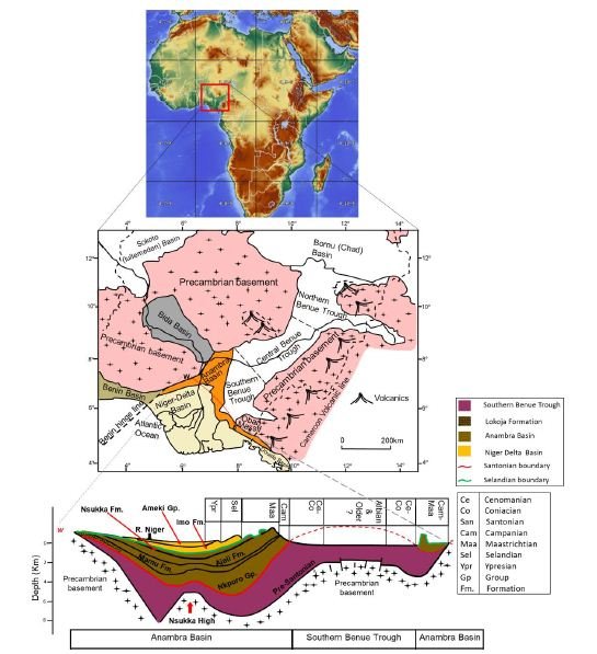
The Benue Trough is a NE-SW trending depression approximately 1000 km by 100 km in dimension, which comprises a suite of depocenters broadly grouped into Northern, Central and Southern Benue Trough (Figure 1) [18,19]. It is part of a much larger west and central rift system (WCARS) that formed due to stresses arising from the opening of the South Atlantic Ocean in the Barremian age [18-23]. The opening of the Equatorial Atlantic Ocean consequent upon the final separation of the African plate from the South American plate in the Albian [24] resulted in flooding of the Southern Benue Trough, leading to the deposition of the Asu-River Group. Due to global sea level rise, this flooding, which peaked in the Cenomanian-Turonian boundary con Turonian tinued into the Turonian [25,26], were floodwaters from the equatorial Atlantic Ocean connected with floodwaters from the Tethys Ocean to establish the Trans-Saharan seaway through the Benue Trough. This resulted in the deposition of the Eze-Aku and Awgu groups [10,27]. The Eze-Aku and Awgu groups belong to one depositional episode spanning latest Cenomanian to Coniacian [27]. Gebhardt [28] reported that these units could only be differentiated based on fossil content. In the southern Benue Trough, the Eze-Aku group comprises chiefly of highly fossiliferous calcareous mudstone intercalated with sands, and limestone units deposited in environments ranging from continental to deep marine environments [29-36]. The Awgu Group consists of limestone, mudstone interstratified with thin limestone and marl units [27], as well as subordinate sands. Coal units have been documented at the top of the stratigraphic succession. These units are interpreted to have been deposited in delta plain to marine conditions [10,19,28]. The Trans-Saharan Seaway was short lived and eventually broken in the Santonian primarily due to a change in stress regime, which brought about reactivation of NE-SW trending faults, folding, volcanism as well as exhumation of pre-Santonian strata of which the southern Benue trough was the most affected [37]. After the Santonian inversion, came a phase of renewed subsidence west of the Southern Benue Trough, which formed the Anambra Basin. The Anambra Basin (Figure 1) represents the sag phase of the Benue Trough evolution. The oldest and youngest parts of its lithic fill comprises the Nkporo Group whose facies is dominantly marine, but shows fluvial to fluvio-marine character at the marginal parts of the basin [6,19] and the brackish Nsukka respectively.

Figure 1: Map of Nigeria showing areas underlain by sedimentary and basement rocks. Below is a W-E cross section showing lithostratigraphic packages of southern Nigeria ranging from Barremian to Ypresian (Edegbai et al., 2019b).

The Mamu Formation comprises mudstone, sand, limestone, carbonaceous and calcareous mudstone, as well as coal and minor ironstone units, which exhibit spatio-temporal variability with respect to thickness and facies [9,36,38,39] Simpson in [19,31,40]. In recent times, these units have been adduced to represent estuarine to shallow marine depositional conditions [9,36,39]. In addition, variable ages ranging from middle Maastrichtian in the North (Gebhardt, 1998) – 22 to late Campanian to middle Maastrichtian in the South implying later sedimentation of the Mamu in northern Anambra-Basin have been reported (Figure 2) [31,38,40,41].

Materials and Methods

Elemental Analysis

Ninety drill cuttings and core samples from the Nzam-1, Idah-1, Owan-1, Amansiodo-1 wells (Figure 3a-3g) representing the post-Santonian Mamu Formation as well as the pre-Santonian Eze-Aku and Awgu groups were obtained from the Nigerian Geological Survey Agency storage Core Repository at Kaduna, Nigeria. A combination of cluster and systematic sampling techniques (modified by sample availability and stratigraphic control based on well logs and original reports from oil companies) was employed. Sample preparation entailed homogenization and mechanical pulverization into powder, succeeded by near total multi-acid digestion and elemental analysis using ICP-MS at Activation Laboratories, Ontario, Canada.

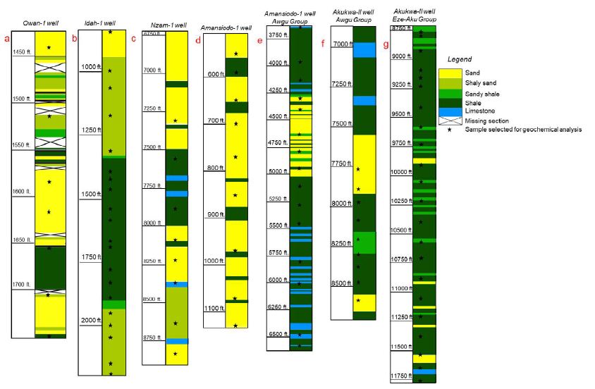
Figure 3: a-d, Lithology of the Mamu Formation penetrated by Owan-1, Idah-1, Nzam-1 and Amansiodo-1 wells respectively. e-f, Lithology of the Awgu Group penetrated by the Amansiodo-1 and Akukwa-II wells. g, Lithology of the Eze-Aku Group penetrated by the Akukwa-II well. See Edegbai, et al., (2019b) for the lithology of outcropping units of the Mamu Formation on the western margin.

Results

The results of major and trace element analysis were integrated before comparison with previously generated data from outcrops located at the western flank of the Anambra Basin by the authors [some of which have been published [9] as well as data from the eastern margin [13]. As observed [42], argillaceous sediments and fine sands better preserve the provenance signature of source units than coarser units. Consequently, for the purpose of our study, only data from the outcropping dark mudstone lithofacies in the western flank, which has been subdivided into marsh, bay and central basin subenvironments in order of proximality [9], was integrated with data from the drill cuttings. A summary of the elemental analysis results is presented in Appendix 1a-c.

Major Elements (Ca, Fe, Mg, Mn, Ti and Al)

Outcropping Mamu Formation

On the western margin, Al and Fe are the most abundant major elements in the sediment samples (Appendix 1a, Figure 4a-b). 65.2 %, 95.7 %, 96.1 % of samples from the marsh, bay and central basin subenvironments are above the average upper continental crust [43] limit for Al. All samples from the marsh subenvironment have concentrations below the UCC limit for Fe (UCC = 3.5 %), whereas 50 % and 91.3 % of the samples from the central basin and bay subenvironments, respectively fall below the UCC limit for Fe. While all samples have concentrations below the UCC limits for Ca, K, Mg, and Na (UCC = 3 %, 2.8 %, 1.33 %, and 2.89 % respectively), the Ti concentrations are above the UCC composition (UCC = 0.41 %) (excluding one outlier from the central basin subenvironment). Outcrop data [13] for the eastern margin suggests that Al and Fe are the most abundant major elements (Appendix 1a, Figure 4a-b). The concentrations of Ca, K, Mg and Na concentration in the samples are below the respective UCC limits. 88.9% and 66.7% of the samples have Al and Fe concentrations below the respective UCC, while all the samples have Ti concentration above the UCC for Ti (Appendix 1a, Figure 4a-b). In broad terms, the more distal and saline central basin subenvironment shows the highest concentration of Ca, Fe, K, Mg, Mn, Na and Al in all the dark mudstone samples (Appendix 1a, Figure 4a-b). These are very similar in their median values to those reported [13] (Appendix 1a, Figure 4a-b), whereas the lowest concentrations are recorded from the more proximal less saline marsh subenvironment (Appendix 1a, Figure 4a-b).

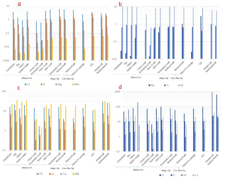
Figure 4: Variograms showing the median concentrations of major and high field strength elements for all sample locations as well as regional data from western and northcentral Nigeria (Lapworth et al., 2012).

Well Data

Mamu Formation

Aluminium and Fe are the most abundant among the major elements (Appendix 1a, Figure 4a-b). In the Owan-1 well, all samples are below the UCC limits for Ca, Fe, K, Mg, and Na, while 71.4 % and 14.3 % of the samples have concentrations above the respective UCC limits for Ti and Al. All samples from the Amansiodo-1 well have Fe, Ti, Al, K, Mg, and Na concentrations below the respective UCC limits. In addition, 33.3% of the samples have Ca concentration above the UCC limit. All the samples from the Idah-1 and Nzam-1 wells have concentrations below the UCC limits for Ca, K, Mg and Na. Furthermore, all the samples from the Nzam-1 well have Ti concentrations above the UCC limit, as do bulk of the samples (90.5%) from the Idah-1 well. With respect to Fe and Al concentrations, 87.5% and 75% of samples from the Nzam-1 well, as well as 85.7% and 61.9% of samples from the Idah-1 well have Fe and Al concentrations greater than the respective UCC. The data from Amansiodo-1 (closest to the eastern boundary) and the Owan-1 (on the western margin) wells show very distinct major element distribution in comparison to results from the more central Nzam-1 and Idah-1 wells. The Amansiodo-1 samples possess the largest median concentrations of Ca as well as much lower concentrations of the other major elements. The median values of the major element data from Owan-1 are very comparable with the marsh outcrop samples, which are also depleted in Ca and Mg (Appendix 1a, Figure 4a-b). The samples from Idah-1and Nzam-1 wells show greater Ca, Fe, K, Mg, Mn, Na and Ti concentrations (Appendix 1a, Figure 4a-b), in comparison to data from the marginal wells. Furthermore, the Idah-1 well also shows subtle variation in major element concentration when compared to the southern Nzam-1 well. Greater concentrations of Ca, Mg, Mn and Ti abound in the Idah-1well in comparison to the Nzam-1 well, which shows greater concentrations of K, Na and Al (Appendix 1a, Figure 4a-b).

Pre-Santonian Units.

Aluminum and Fe are the most abundant major elements in the samples from the Awgu Group (Appendix 1a, Figure 4a-b). Whereas all samples show Fe, Ti and Al concentrations above the respective UCC limits (except an outlier from the Akukwa-II well), the concentrations of Ca, K, Mg and Na in the samples (except an outlier from the Amansiodo-1 well) remain below their respective UCC limits (Appendix 1a, Figure 4a-b). Furthermore, the major element distribution in the Awgu Group shows slight variability. Whereas samples from the Amansiodo-1 well are slightly more enriched in Fe, K, Ti and Al, the Akukwa-II well samples are slightly more enriched in Ca and Na (Appendix 1a, Figure 4a-b). In the Eze-Aku Group, Al and Fe are the most abundant major elements (Appendix 1a, Figure 4a-b). All the samples show K and Na concentrations below their respective UCC limits, while 85% and 95.2% of the samples have Ca and Mg concentrations below the respective UCC limits. In addition, the concentration of Fe and Al in the bulk of the samples is above the UCC limit. In general, samples from the Eze-Aku Group show slight enrichment in Na and Ca over the samples from the Awgu Group that reveal higher concentrations of Fe, K, Mg, Ti and Al. In addition, the major element distribution in the pre-Santonian units are quite comparable to those observed from the centrally positioned Nzam-1 and Idah-1wells (Appendix 1a, Figure 4a-b).

High Field Strength Elements (HFSE: Th, U, Ta, Nb, Zr, Y, Hf)

Outcropping Mamu Formation

All the dark mudstone samples on the western margin have U and Nb concentrations above the respective UCC limits (UCC for U and Nb = 2.8 ppm and 12.0 ppm respectively) (Appendix 1b, Figure 4c-d). The Th and Ta concentrations of all the samples from marsh and bay subenvironments, and the bulk of the samples (92.3% and 88.5% respectively) from the central basin subenvironment are above the respective UCC limits for Th (UCC = 10.7 ppm) and Ta (UCC = 1 ppm). In addition, a very large proportion of the dark mudstone samples have concentrations below the UCC for Zr and Hf (UCC for Zr and Hf = 190 and 5.8 ppm, respectively). Furthermore, 56.5%, 34.8%, and 38.5% of samples from the marsh, bay and central basin subenvironments respectively have Y concentration above the UCC limit (UCC = 22 ppm). On the eastern margin, data from Odoma et al. (2015), show that all the samples are enriched above the UCC concentration for Th, U, Nb, Zr and Hf (Appendix 1b, Figure 4c-d). In general, with the exception of Zr and Hf, which are much higher, the concentration of the other HFSE being discussed are more comparable to the outcrops at the Benin flank than the well data (Appendix 1b, Figure 4c-d).

Well Data

Mamu Formation

As observed in the major element distribution, the Amansiodo-1 well samples show very distinct geochemical distribution of the HFSE (Th, U, Ta, Nb, Zr, Y, and Hf) as indicated by very low concentrations that are at least one order lower than those obtained from the outcropping units (Appendix 1b, Figure 4c-d). The HFSE abundance from the Owan-1 well, though much higher than the data from the Amansiodo-1 well, is subordinate to the outcropping units (Appendix 1b, Figure 4c-d). In the more centrally located Nzam-1 and Idah-1wells, a very large proportion of the samples show enrichment in Th, U, Ta, and Nb above the respective UCC (Appendix 1b, Figure 4c-d). In the Idah-1 well, 57%, 85.7% and 28.6 % of the samples have concentration above the respective UCC for Zr, Y, and Hf (Appendix 1b, Figure 4c-d). The Zr, Y and Hf concentrations that are higher than the outcropping units on the western margin are subordinate to the Zr and Hf on the eastern margin [13]. By contrast, the outcropping units on the western margin show more enrichment in Th, U, Ta, and Nb than the sediments in the Nzam-1 and Idah-1wells (Appendix 1b, Figure 4c-d). Furthermore, with the exception of Th, the median concentrations of the HSFE being discussed decreases from samples from Idah-1 well location to the samples from Nzam-1 well (Appendix 1b, Figure 4c-d). In the Nzam-1 well, the bulk of the samples, which show enrichment in Th, U, Ta and Nb above the respective UCC limit, show depletion in Zr, Y, and Hf concentrations.

Pre-Santonian units

The Awgu Group samples from the Amansiodo-1 well show more enrichment in Th, U, Ta, Nb, Zr, Y and Hf in comparison to samples from the Akukwa-II well (Appendix 1b, Figure 4c-d). The median values of the HFSE are comparable to the Mamu Formation data from the Idah-1and Nzam-1 wells. In addition, a large proportion of the samples from the Amansiodo-1 well show enrichment above the respective UCC for Th, U, Ta and Nb and Y (Appendix 1b, Figure 4c-d). Conversely, the samples are depleted below the respective UCC composition for Zr and Hf (Appendix 1b, Figure 4c-d). A much lower proportion of the samples from the Akukwa- II well show enrichment above the respective UCC limits for U, Ta, Nb and Y. Furthermore, none of the samples are enriched above the UCC concentrations for Th, Zr and Hf (Appendix 1b, Figure 4c-d). In broad terms, when compared with the post-Santonian Mamu Formation (excluding the samples from Owan-1 well and the Amansiodo-1 well), the Awgu Group is depleted in Th, U, Ta, Nb, Zr and Hf concentrations (Appendix 1b, Figure 4c-d). In contrast, the concentration of La and Y is much higher than in post-Santonian units (Appendix 1b, Figure 4c-d). The bulk of the samples from the Eze-Aku Group show depletion in Th, U and Hf concentrations below the respective UCC composition (Appendix 1b, Figure 4c-d). In addition, none of the samples show enrichment in Zr and Hf above the respective UCC limits (Appendix 1b, Figure 4c-d). Conversely, a larger proportion of the samples are enriched in Ta and Nb above the respective UCC limits. The HFSE distribution within the Eze-Aku Group is very comparable to the data from the Awgu Group in the Akukwa II well, except that much lower Zr concentrations are present (Appendix 1b, Figure 4c-d).

Transition Trace Elements [(TTE) Ni, Co, V, Cr and Sc)]

Outcropping Units

A large proportion of the marsh and bay samples are depleted in Ni, Co and Sc content. Conversely, the bulk of the samples show enrichment in Cr (Appendix 1b, Figure 5a-b). There is a distinction in the V content of the marsh and bay samples. Whereas the bulk of the Marsh samples are enriched above the UCC limit for V (UCC = 107 ppm), only 8.7 % of the Bay samples show V enrichment above the UCC limit. In comparison to the marsh and bay units, the central basin samples are much more enriched in TTE, only subordinate to the marsh unit in V concentration (Appendix 1b, Figure 5a-b). On the eastern margin, data [13] shows depletion of Ni and Co, whereas a substantial proportion of the samples show enrichment above the Cr and Sc of the respective UCC composition (UCC = 83 ppm and 13.6 ppm, respectively) (Appendix 1b, Figure 5a-b). In addition, 44.4% of the samples are enriched above the UCC mean for V. In general, the central basin unit shows the most enrichment in TTE when compared with the other outcrop units (Appendix 1b, Figure 5a-b), which is perhaps due to the redox conditions prevailing. The V and Cr content in the eastern margin is much lower than the marsh and central basin units in the western margin are (Appendix 1b, Figure 5a-b). Furthermore, excluding the central basin unit, all other outcrop samples are depleted in Ni and Co concentrations (Appendix 1b, Figure 5a-b).

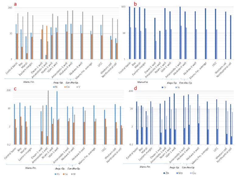
Figure 5: Variograms showing the median concentrations of TTE as well as Pb, Sn, W, Zn, Mo, and Cu for all sample locations as well as regional data from western and northcentral Nigeria (Lapworth et al., 2012).

Well Data

Mamu Formation

The TTE distribution in samples from the Owan-1 and Amansiodo-1 wells are very distinct from the more centrally located wells due to their lower TTE concentrations. The samples from the Nzam-1 well show significant enrichment above the samples from the Idah-1well (Appendix 1b, Figure 5a-b). The Ni concentration in majority of the well samples are below the UCC limit (UCC = 44 ppm). In addition, while the V, Cr and Sc abundances of all samples from the Owan-1 and Amansiodo-1 wells as well as the majority of the samples from the Idah-1well fall below the respective UCC composition (Appendix 1b, Figure 5a-b), the Co content in the majority of the samples are above the UCC mean (UCC = 17 ppm). In general, the outcropping units on the western margin contain higher levels of V, Cr and Sc than their well counterparts (Appendix 1b, Figure 5a-b).

Pre-Santonian Units

Excluding the Cr concentration, which is depleted in the samples from Akukwa – II well, the TTE distribution in the Awgu Group is quite similar with a dominance of samples enriched above the respective UCC limits. Excluding the Ni concentration, which are much lower, the Eze-Aku unit shows similar distribution of TTE with those of the Awgu Group in the Akukwa –II well (Appendix 1b, Figure 5a-b). In broad terms, higher V, Co, Ni, and Sc concentrations persist in the pre-Santonian units when compared with the Mamu Formation, which is more enriched in Cr.

Pb, Sn, W, Zn, Mo and Cu Bivalent Metals

Outcropping Mamu Formation

The marsh unit contains significantly lower Pb, Sn, Zn and Cu concentration when compared with the bay and central basin units (Appendix 1a, Figure 5c-d). The bay unit shows more enrichment in Pb, Sn, Mo and W when compared with the central basin unit that has a much higher Zn concentration (Appendix 1a, Figure 5c-d). A large proportion of the central basin samples have Sn, W, Mo and Zn below the respective UCC limits (UCC = 5.5 ppm, 2 ppm, 1.5 ppm, and 71 ppm, respectively), whereas 58% of the samples show enrichment in Cu above the UCC limit (UCC = 25 ppm). In addition, sizeable proportions of the marsh samples have W, Zn, and Cu below the respective UCC limits, whereas a majority of the bay samples shows enrichment in W, Mo, and Cu as well as depletion of Zn when compared with the respective UCC means. Furthermore, all the samples show enrichment in Pb above the UCC limit (UCC = 17 ppm), whereas a sizeable proportion show enrichment in Mo above the UCC limit. On the eastern margin [13], all the samples show enrichment in Pb above the UCC limit (Appendix 1a, Figure 5c-d). In addition, 53% and 26% of the samples show enrichment in Zn and Cu, respectively, when compared with the UCC. In general, the outcropping units along the western margin show higher levels of Pb and Sn than the eastern margin, which shows more enrichment in Zn (Appendix 1a, Figure 5c-d).

Well Samples

Mamu Formation

All the well samples show enrichment at or above the UCC concentration of W, whereas the bulk of the well samples show depletion in Mo. Excluding a few samples from the Idah-1well, all others are depleted in Sn and Cu when compared with the respective UCC average (Appendix 1a, Figure 5c-d). A very large proportion of the samples from the Idah-1and Nzam-1 wells shows enrichment above the UCC limits for Pb and Zn (Appendix 1a, Figure 5c-d). The samples from Idah-1well in particular shows very high levels of Pb and Zn as well as Sn in some intervals. The Owan-1 and Amansiodo-1 wells show some distinction, as a large proportion of the samples from both wells is depleted in Zn when compared with the centrally located wells (Appendix 1a, Figure 5c-d). In addition, all the samples from the Amansiodo-1 well show enrichment above the UCC for Pb, whereas only 28.6% of samples from the Owan-1 well have Pb concentration above the UCC.

Pre-Santonian Units

All the samples from the Awgu Group across the wells are enriched in Pb, W and Zn above the respective UCC, whereas by contrast, are depleted in Sn (Appendix 1a, Figure 5c-d). The samples from Akukwa-II well show higher levels of Zn, W, Mo and Cu, thus contrasting with samples from the Amansiodo-1 well. In addition, nearly all the samples from the Akukwa-II well are enriched above the UCC limits for Mo and Cu, whereas a lower proportion of samples from the Amansiodo-1 well (60% and 53.3% respectively) are enriched above the respective UCC. A very large proportion of the samples from the Eze-Aku Group show enrichment in Pb, W, Zn, Mo, and Cu, whereas all the samples are depleted in Sn (Appendix 1a, Figure 5c-d). In addition, the Eze-Aku group is more enriched in Mo, W, and Zn when compared with samples from the Awgu Group. In general, the pre-Santonian units show enrichment in W, Zn, Mo, and Cu when compared with data from the post-Santonian Units (Appendix 1a, Figure 5c-d). There is significantly more enrichment of Pb in the Mamu Formation when compared with data from the pre-Santonian Awgu and Eze-Aku Groups.

Discussion

Degree of Chemical Alteration

The order of stability of major elements as suggested [44] implies that Si, Fe, Ti and Al are the most stable elements. Thus, the proportion of major elements can provide some clues as to the degree of chemical alteration in the source region. The most depleted elements are Na, Ca, and Mg indicative of a high degree of initial weathering, except in the case of the Eze-Aku Group in the Akukwa-II well and the Mamu Formation in Amansiodo-1 well that are enriched in non-silicate Ca. Na/K, Mg/K, K/Al and Na/Al, which reflects the proportion of less stable minerals like plagioclase, biotite, chlorite, smectite, vermiculite and illite relative to more stable K-feldspar, illite and Kaolinite has been shown to track the degree of weathering of crustal material [45]. A higher degree of chemical alteration is inferred for the outcropping units on the western and eastern margins as well as the samples from the Owan well based on the low Na/Al, K/Al, Mg/K and Na/K. This is illustrated further by the major element distribution [(Na, Ca, Mg) <K<Ti<Fe<Al] as well as low Mg/Ti (Appendix 1a, c Figure . 4a-b, 6a-c). In addition, higher Na/Al, K/Al, Mg/K (Appendix 1c, Figure 6c) recorded for the central basin mudstones as well as the samples from the eastern margin [13] suggests relatively lower degrees of chemical alteration. This is adduced to authigenic illite and smectite formation arising from an increase in salinity [9]. Furthermore, in comparison with the outcropping units, data from the Amansiodo-1 well as well as the more centrally placed Nzam-1 and Idah-1wells show much higher Na/Al, K/Al, Mg/K, Na/K, Mg/Ti values (Appendix 1c, Figure 6c). This indicates a lower degree of chemical alteration regardless of carbonate dilution (calcite cement) in the Amansiodo-1 well (Na<K<Mg<Ti<Al<Fe <Ca) that has modified the major element distribution pattern. We hypothesize that the higher salinities in these areas as suggested by early Maastrichtian paleogeographic reconstruction [6] may account for some increment in the Na/Al, K/Al, Mg/K, Na/K, Mg/Ti values as well as the extent of mixing from provenance regions (discussed in section 5.3). In addition, data from the eastern margin as well as the central basin mudstones, which show higher K relative to Ti (which increases with higher Mg/Ti) further illustrates this. The data from the Awgu Group is comparable to those observed in the Nzam-1 and Idah-1 wells) except in Mg/Ti, which is much higher (Appendix 1c, Figure 6c). The observed major element trend (Ca<Na<Ti<Mg<K<Fe<Al) at the Amansiodo-1 well is distinct from that of the Awgu (Ca<Ti<Na<Mg<K<Fe<Al) and Eze-Aku (Ti<Mg<Na<K<Ca<Fe<Al) groups observed at the Akukwa-II well, which have lower Ti relative to Na, Mg and K (Appendix 1a, Figure 4a-b, 6c). This implies a higher degree of chemical alteration of the Awgu Group in the Amansiodo well. In general, regardless of carbonate dilution in the samples from the Eze-Aku Group, we can infer that a much lower degree of chemical alteration and consequently mineralogical immaturity persists in the pre-Santonian units when compared with the Mamu Formation. This is based on the much higher Na/Al, K/Al, Mg/K, Na/K, Mg/Ti (Appendix 1c, Figure 6c), as well as higher percentages of smectite, illite and mixed layered clays reported for these units, in comparison to those reported for the Mamu Formation [7,9,27]. Furthermore, our findings are consistent with published results of petrographic analysis, which reported textural and mineralogical immaturity of the pre-Santonian units as distinct from the more texturally and mineralogically mature post-Santonian units of which the Mamu Formation subsists [3,5,7,46]. This is in spite of the humid equatorial climatic conditions that prevailed at during the Cenomanian-Turonian and Campanian- Maastrichtian stages [47].

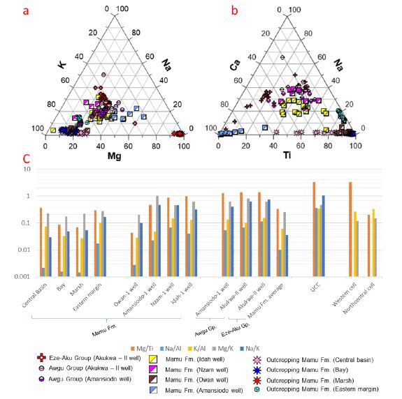
Figure 6: Ternary plots showing the distribution of K, Na, Mg, Ca, Na and Ti concentrations of all sample locations as well as a variogram of median values of Mg/Ti, Mg/K, Na/Al, and K/Al.

Source Rock Composition

Some trace elements common to felsic and mafic rocks have reduced mobility when subjected to weathering, erosion, transportation, and diagenesis [48-53]. Consequently, their concentrations in sedimentary rocks can give valuable insight in provenance studies [52]. To reduce the uncertainty regarding the accuracy of provenance determination using trace elements, we utilized trace elements whose concentrations are least affected by redox conditions. We assume that the concentration of these conservative trace elements in our samples preserve the geochemistry of the sediment provenance regions. The Th/Sc vs. La/Sc, TiO2 vs. Zr, Th/Sc vs. Sc, as well as Th/Sc vs. Zr/Sc discriminant plots [50,52] (Figure 7a-h) highlight intra- and interformational variation in the geochemical characteristics of the pre-Santonian units and the Mamu Formation, which are useful in determining the chemical composition of source units.

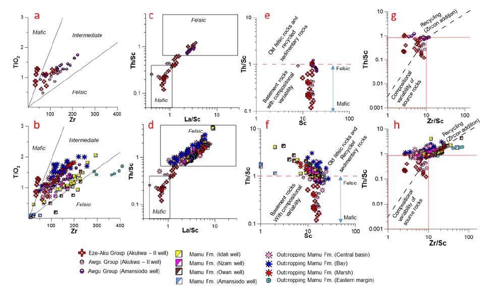
Figure 7: TiO₂ vs. Zr (a-b) (after Hayashi et al., 1997), Th/Sc vs. La/Sc (c-d) (after Cullers, 2000) and binary plots showing source composition of the pre-Santonian units as well as the Mamu Formation. Th/Sc vs. Sc (after McLennan and Taylor, 1991) (e-f) and Th/Sc vs. Zr/Sc (g-h) (McLennan et al., 1993) binary plots indicate variable basement sources for pre-Santonian strata as well as a combination of felsic basement rocks and recycled pre-Santonian strata sources for the Mamu Formation.

Pre-Santonian Units

Samples from the pre-Santonian units show a uniform Sc concentration (averaging ~ 15ppm) (Figure 7e-f), whereas the Th, Zr and La content of these units are highly variable (Figure 7a-h, Appendix 1b). The geochemical characteristics of the pre-Santonian units suggests a basement source rock with compositional variability as shown by the Th/Sc < 1 (Figure 7c-f) [50]. This is illustrated further by the Th/Sc vs. Zr/Sc binary plot [54] (Figure 7g-h), which indicate that these units were not sourced from reworked older sedimentary rocks. Intraformational compositional variability is visible in the Awgu Group (across the Amansiodo-1 and Akukwa-II wells) as well as the Eze-Aku Group. In the Akukwa-II well, a mafic to intermediate source rock composition is inferred due to the much lower Th, Zr, La and other HFSE concentrations, whereas in the Amansiodo-1 well, which has much higher concentration of HFSE, an intermediate to felsic source rock composition is inferred (Appendix 1b, Figure 4c-d, 7a-d). The observed spatial variation in degree of chemical alteration in the Awgu group (highlighted in section 5.1) is in part due to the more felsic nature of the source rocks for the sediments from the Amansiodo-1 well. The Eze-Aku unit shows source rock composition varying from (predominantly) mafic to felsic basement rocks owing to a range of Th, Zr, and La concentrations, which are the lowest among the pre-Santonian units (Appendix 1b, Figure 4c-d, 7a-d).

Mamu Formation

Samples from the pre-Santonian units show a non-uniform Sc concentration as well as variable Th, Zr, and La concentrations. This depicts a (predominant) felsic to intermediate source composition (Figure 7b, d, f) hypothesized to be derived from reworked pre-Santonian units as well as (predominantly) silica rich igneous and metamorphic rocks. Evidence for recycling of pre-Santonian units is illustrated by a higher degree of chemical alteration (see section 5.1), low index of compositional variability [9], a large proportion of the samples having Th/Sc > 1 (characteristic of recycled sedimentary rocks), as well as inferences from Th/Sc vs. Zr/Sc and Th/Sc vs. Sc (Figure 7f, h) discriminant plots [50,54]. In addition, the better textural and mineralogical maturity reported for the post-Santonian units [3,5,7,46] is attributable to a significant proportion of their provenance originating from reworked pre-Santonian units. Furthermore, Th/Sc < 1 reported for some samples (Appendix 1c), inferences from Th/Sc vs. Zr/Sc and Th/Sc vs. Sc (Figure 7f, h) discriminant plots [50,53], as well as variability in the degree of chemical alteration (discussed in section 5.1) provides evidence for detrital contribution from silica rich igneous and metamorphic rocks. This is further illustrated by the high concentration of W reported for the sediments (especially in the Owan-1, Amansiodo-1 and Idah-1 wells) (see section 5.3), which are much higher than those recorded for the pre-Santonian units points to detrital contribution from basement rocks, as W is not known to survive several weathering and sedimentation cycles [17].

Provenance

Leveraging on the reports of geochemical observations of the north central and southwestern basement complex, as well as Pb-Zn deposits in southern Benue trough [12,17], we attempted to work out the dominant source regions in different parts of the Anambra Basin during the late Campanian to early Maastrichtian time.

Three of the factors controlling element associations, which were identified by Lapworth, proved to be quite useful in this study. These are:

a) An iron-oxide/hydroxide and ilmenite factor, which explains the low to moderate positive covariation between Fe and Cu, Cr, Mo, V, Zn, Co, Sn, and Ti. The presence of ilmenite allows for a positive covariance between Fe and Ti or Sn;

b) A mafic factor, which explains the positive covariation between Fe, Mn, and Mg due to the presence of ferromagnesian minerals such as olivine, pyroxene, hornblende, and biotite;

c) A coltan factor. Coltan abundance covaries positively with Ta, Nb, Ti, Sn, and W.

Mamu Formation

On the western margin, the outcropping units show a broad Pb-Zn covariation (Figure 8a-c), as well as an enrichment of Pb over Zn (Pb/Zn > 1) (Appendix 1c). There is a moderate influence from moderate Fe-oxide/hydroxide factor, which is observed only in the more proximal marsh unit as well as a strong to moderate coltan influence for Sn and W as shown by the positive Sn and W covariation with Nb, Ta and Ti (Figure 8a-c). The Sn vs. Pb and W vs. Pb show a broad distribution in the bay unit, whereas a moderate positive covariation is observed in the central basin and marsh units (Figure 8a-c).

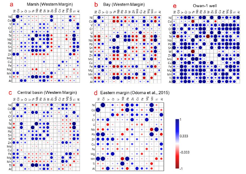
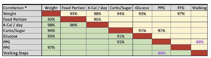
Figure 8: Correlation matrix for major and element abundances in sediments of the Mamu Formation on the western and eastern margins as well as the Owan-1 well.

On the eastern margin, a weak positive Pb-Zn covariation exists with Pb/Zn < 1. In addition, there is a strong influence from the mafic factor as well as a minimal influence from the Fe-oxide/hydroxide/ilmenite factor. The absence of Sn and W data prevents a discussion of the coltan factor. However, a moderately positive Pb vs. Nb covariation (Figure 8d) suggests some potential influence by the coltan factor. There is a coltan source, which exerts a minor influence on the distribution of Ti, Sn, and W in samples from the Owan-1 well (Figure 8e). By contrast, the distributions of Sn and W are strongly controlled by the ilmenite factor as shown by the strong positive covariation of Ti with Sn, Fe and W (Figure 8e). There is also a moderate influence from a mafic source as well as a good Pb-Zn covariation (Pb/Zn < 1). In the Amansiodo-1 well, there is a moderate mafic factor influence, a broad Pb-Zn covariation (Pb/Zn <1), as well as a strong Fe-oxide/hydroxide/ilmenite factor (Figure 8e). In contrast to the sediments from the Owan-1 well wherein a moderate positive covariation of Pb vs. Sn is observed, the sediments from the Amansiodo-1 well show a broad Pb vs. Sn covariation as well as a moderate positive coltan influence for Ti and Sn (Figure 9a). Furthermore, in the Owan-1 well there is broad W vs. Pb covariation as well as good W vs. Zn covariation (Figure 8e), whereas the Amansiodo-1 well there is a good positive W vs. Pb covariation as well as a moderate positive W vs. Zn covariation (Figure 9a).

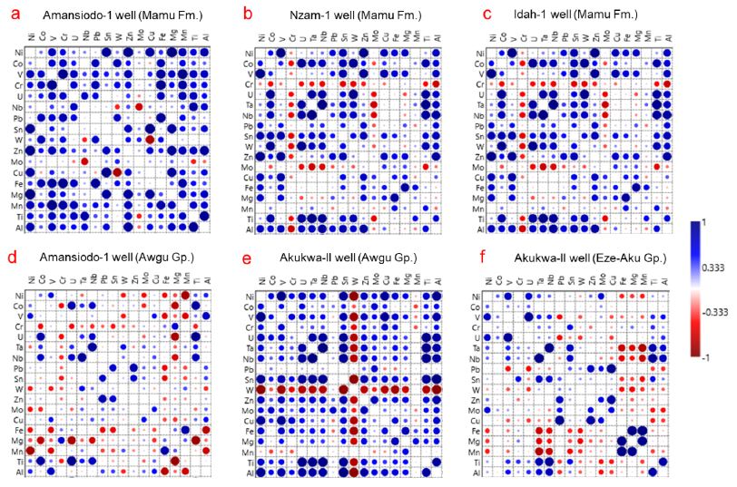
Figure 9: Correlation matrix for major and element abundances in sediments of the Mamu Formation and pre-Santonian units.

The Pb vs. Zn shows a poor covariation in sediments from the Idah-1well (Pb/Zn >1), which becomes moderate in the Nzam-1 well (Pb/Zn>1) (Figure 8b-c). The influence of a coltan source for Sn and W improves from being weak in the Idah-1 well samples to moderate in the Nzam-1 well samples (Figure 8b-c). In addition, the influence of the mafic factor as well as the Fe-oxide/hydroxide factor is moderate in samples from these wells (Figure 8b-c).

Awgu Group

As observed earlier, this unit exhibits strong spatial geochemical variability. In sediments from the Amansiodo-1 well, the Fe-oxide/hydroxide/ilmenite influence is minimal to non-existent (Figure 9d). There is also a strong mafic component as well as good positive Pb-Zn covariation (Figure 9d) (median Pb/Zn = 0.23). Conversely, the sediments from Akukwa-II well show a moderate positive Pb-Zn covariation (median Pb/Zn = 0.17), as well as a fair to strong influence from the mafic and Fe-oxide/hydroxide/ilmenite factors (Figure 9e). Furthermore, whereas the sediments from the Akukwa-II well show a strong positive covariation of Ta with Sn as well as a strong negative covariation of W with Ta (Figure 9e), the sediments from the Amansiodo-1 well show the opposite. This is illustrated by the moderate covariation of Ta with W as well as a strong negative covariation of Sn with Ta (Figure 9d).

Eze-Aku Group

In the Eze-Aku Group, the influence of the coltan, mafic, as well as the Fe-oxide/hydroxide components are strong (Figure 9f). Sn moderately covaries positively with Nb, Ta, and Ti, whereas W shows a broad to moderately negative covariation with Nb, Ta and Ti (Figure 9f). There is a good positive Pb-Zn covariation (median Pb/ Zn = 0.22). In general, the pre-Santonian units show a stronger mafic influence as well as a stronger Pb-Zn covariation, which is a function of the composition of the source rocks (section 5.2).

Differentiation of Provenance Regions

Pre-Santonian Units

Based on field observations, petrographic studies and paleocurrent measurements, earlier studies favoured the granites, gneisses and metasediments in the eastern highlands and southwestern basement complex of Nigeria (Figure 2) [5,7,9,46] as the provenance sources for the pre-Santonian units. The identification of a dominant mafic provenance for the Eze-Aku unit from our data (Figure 7a, c, e), which is strengthened by the strong mafic factor influence as illustrated by the strong positive covariation between Fe vs. Mg, Fe vs. Mn as well as negative covariations of Fe vs. Pb and Fe vs. Sn (Figure 9f) Lapworth is quite an interesting find as this has only been advanced for the Asu-River Group [7]. The basement complex in the eastern highlands have been adduced to be the provenance for the Awgu and Eze-Aku groups in the eastern segment of the Anambra Basin [7,34]. However, we hypothesize a significant detrital contribution from the mineralized biotite granites as well the basement complex rocks of north central Nigeria (Figure 10a-b) due to the Nb, Ta and W that are above the respective UCC as well as Sn (Appendix 1a-b, Figures 4c and 5c). A strong detrital contribution from north central Nigeria is adduced to be responsible for the distinct geochemical character observed in the sediments from Amansiodo-1 well in comparison to the Akukwa-II well. This is illustrated by the more felsic character or the sediments, higher degree of chemical alteration, higher Th, U, Nb, Ta, Sn (Figures 4c and 5c, Appendix 1a-b), higher enrichment of Nb over Ta [16], as well as inference from the Nb/W vs. Nb/Ta bivariate plot (Figure 10a). Conversely, the sediments from Akukwa-II well, which show a higher W (Figure 5c) as well as the strong negative to broad Ta vs. W covariation (Figure 9e-f) strongly suggests a large proportion of detrital contribution from the eastern highlands (Figure 10a-b) whose pegmatites are enriched in W, but barren with respect to Sn, Ta and Nb [55,56].

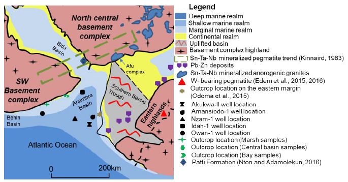
Figure 2: Conceptual early Maastrichtian paleogeographic model with sample locations, ore deposits and mineralized granites or pegmatites.

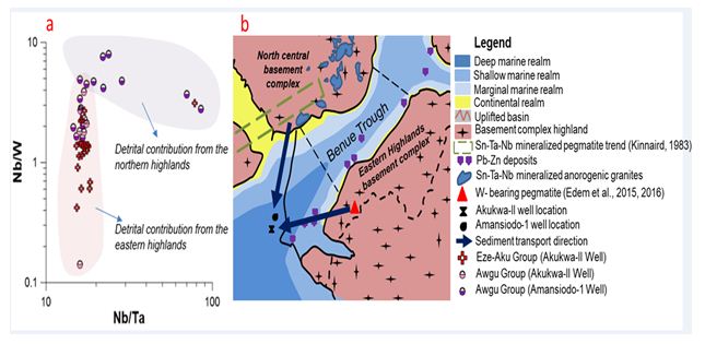
Figure 10: a, Nb/W vs. Nb/Ta binary plot differentiating provenance regions of pre-Santonian units. b, conceptual early Turonian paleogeographic model showing contribution from eastern and northcentral highlands.

Furthermore, we hypothesize a spatio-temporal variation in detrital contribution from the various lithostratigraphic units that make up the eastern highlands and north central Nigeria. Detrital contribution was more from mafic rocks in the latest Cenomanian to early Turonian, whereas from middle Turonian to Coniacian the detrital contribution was more from felsic sources (Figure 7a-f). This is consistent with the findings [7].

Mamu Formation

From the geochemical characteristics highlighted above, we hypothesize that the Mamu Formation is sourced from basement complex rocks as well as recycled pre-Santonian strata. In addition, we can distinguish three broad provenance regions: a Northern provenance, Western provenance, and an Eastern provenance (Figure 11).

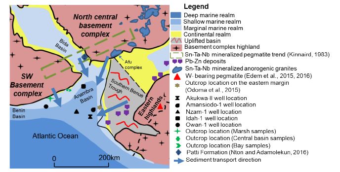
Figure 11: Provenance regions of the Anambra Basin

Western Provenance Region

This region comprises the southwestern basement complex rocks as well as pre-Santonian units, relics of which exist as inliers within the basement complex rocks (Figure 11). In general, this provenance region is characterized by a strong coltan factor controlling the enrichment of Nb, Ta, Sn, W (and Pb to a certain extent), high levels of Th, U, Ta, Nb, Sn, Pb as well has higher Pb/Zn (Pb/Zn >1) when compared to the eastern province. Leveraging on published data [8], the main difference between the western provenance terrain from those of the southwestern portion of the north central province is the much higher Pb abundance, which is consistent with the findings of Lapworth. There is some variability in the element pattern of the western provenance, as a portion of it is not strongly influenced by the coltan factor as shown by much lower Pb, Sn, Nb, Ta, and Y concentrations, lower Pb/Zn (Pb/Zn < 1), as well as much higher W recorded from sediments of the Owan-1 well. The very weak positive covariation for Nb vs. Ti and Nb vs. Sn illustrate further evidence for this (Figure 8e). In addition, the good positive covariation between Ti vs. Sn suggests an alternative source for Ti instead of coltan, which is suspected to be ilmenite Lapworth as well as minerals in the ilmenite-geikielite (MgTiO3) and ilmenite-pyrophanite (MnTiO3) solid solution series due to good to moderate positive covariation of Ti vs. Fe, Mn, and Mg (Figure 8e). These Titanium bearing minerals have been documented to occur in the southwestern basement complex rocks [57-60].

Eastern Provenance Region

The eastern provenance region (Figure 8) comprises the pre-Santonian strata from the Southern Benue Trough as well as the basement complex rocks from the eastern highlands (Figure 11). In general, higher Zn, TTE, Cu, Mo, and major element (excluding Al and Ti) concentrations, much lower Pb/Zn ratios (Pb/Zn <1), a strong W enrichment [55-56], as well as lower levels of Nb, Ta and Sn in comparison with the northern and western provenance regions characterize the eastern provenance. In addition, there exists a good positive Pb vs. Zn covariation, as well as a less strong coltan influence for Sn, which in contrast with the western provenance region shows a broad or strong negative covariation with W. The much higher major element concentrations characteristic of this provenance region is a function of the strong mafic influence on the sediments.

Northern Provenance Region

The anorogenic biotite granites as well as the basement complex rocks in the north central provenance region is hypothesized to have contributed detritus for sediments in the northern segment of the basin, sediments close to the western margin, the area around the Amansiodo-1 well, as well as intervals within the Idah-1 well. We came to this conclusion because some intervals in the Idah-1 well have W concentration above 23.2 ppm (Fig. 12a), which is the highest W concentration reported for stream sediments draining the southwestern portion of the north central basement complex Lapworth. High levels of W concentration have been reported for the biotite granites in the Afu complex, north central Nigeria [17]. In addition, these units show high levels of Nb, Y, Th, Zn, Ti, and U, higher enrichment of Nb over Ta [16], as well as low V and Pb/Zn (Pb/Zn < 1).

Mixing of Provenance Regions

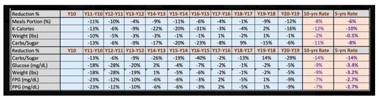
Our published data on the outcropping units on the western margin posit that the marsh samples are the most proximal units of the dark mudstone lithofacies [9]. This implies that the geochemistry of this unit is the least influenced by mixing from the northern and eastern provenance regions. The bay samples are the most affected by mixing as illustrated by higher median concentrations of HFSE as well as Pb, Sn, and W recorded from the bay samples (Figure 12a-d) when compared with the marsh and central basin samples. This is due to contribution from multiple source regions as depicted by the broad distributions of Pb vs. Sn and W vs. Pb (Figure 8b), the fractionation (concentration gradient) of Pb, Nb, W, and Sn between the outcropping Patti Formation (Bida Basin), sediments from the Idah-1 and Owan-1 wells, as well as the outcropping Mamu Formation on the western margin (Figure 12a-d).

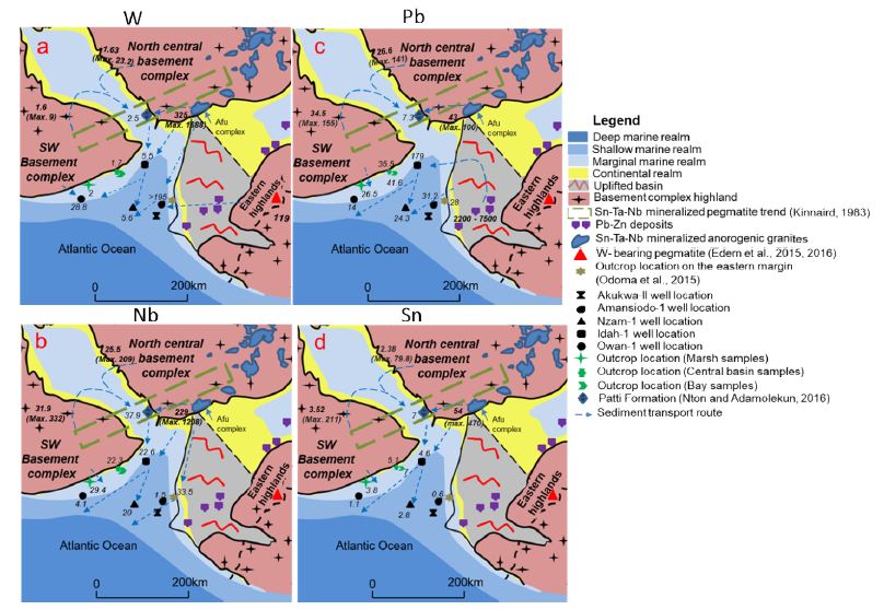
Figure 12: Evidence of mixing of provenance regions deduced from median concentrations of Pb, W, Nb, and Sn from spatial units of the Mamu and Patti formations.

The sediments of the more centrally located Idah-1 and Nzam-1 wells also show clear evidence of mixing of source terrains. This is clearly illustrated by the Pb/Nb vs. Pb/Sn as well as the Pb vs. Sn bivariate plots (Figure 13a-b). We hypothesize that the high Pb values associated with sediments from the Idah-1 well is due to mixing of detritus from all three-provenance regions, as concentrations well above the lower thresholds for Pb and Zn (100 ppm and 200 ppm respectively) in Pb-Zn mineralized regions of the eastern provenance [11,12] abound. In addition, the high levels of W recorded in some intervals in the Idah-1 well as well as the Amansiodo-1 well (Appendix 1a) are within the range reported for the Sn-Nb-Ta mineralized biotite granites of the Afu complex [17] located in the Northcentral provenance region.

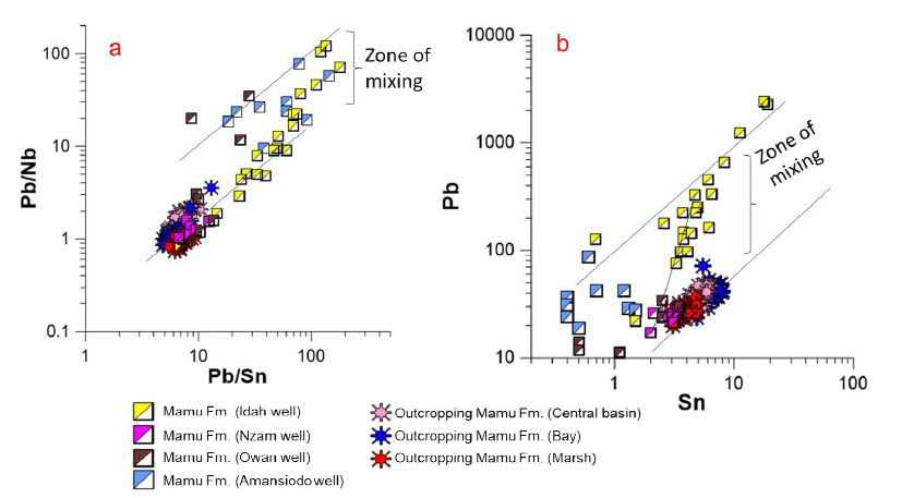
Figure 13: Pb/Nb vs. Pb/Sn (a) and Pb vs. Sn (b) binary plots showing further evidence of mixing of source regions.

Conclusion

This study reports the following findings:

• The pre-Santonian units are sourced from compositionally variable basement complex rocks, ranging from felsic to mafic in composition.
• There is evidence for spatio-temporal variability in the detrital contribution from the basement complex rocks. Detrital contribution was more from mafic rocks in the latest Cenomanian to early Turonian, whereas from middle Turonian to Coniacian the detrital contribution shifted to more felsic sources.
• The provenance of the Mamu Formation is from felsic source rocks comprising of basement complex rocks as well as recycled pre-Santonian rocks. The significant detrital contribution from basement complex rocks provides clear insight regarding to the origin of large sand volumes in the post-Santonian Anambra basin. These hitherto could not be accounted for, due to the predominance of argillaceous and carbonate rocks in the Southern Benue Trough
• Three provenance regions comprising the northern, western, eastern sectors contributed detritus during the Campano-Maastrichtian with evidence of mixing of provenance sources.
• The Mamu Formation shows evidence of secondary Pb, Sn, and W mineral accumulation.

Acknowledgement

This research received support from University of Benin Research and Publications Committee, the Fulbright Commission (15160892), the Niger Delta Development Commission, Nigeria (NDDC/DEHSS/2015PGFS/EDS/011), and DAAD (ST32 – PKZ: 91559388). Julius Imarhiagbe and Reuben Okoliko assisted with fieldwork and sampling of cuttings and core at the Nigerian Geological Survey Agency respectively. In addition, the first author wishes to acknowledge the motivation, guidance and instruction provided by Prof. W.O. Emofurieta and Mr. Sam Coker during the early phase of this research (Table 1a-1c).

References

1. Ladipo KO (1986) Tidal shelf depositional model for the Ajali Sandstone, Anambra Basin, Southern Nigeria. J Afr Earth Sci 5: 177-185.
2. Ladipo KO (1988) Paleogeography, sedimentation and tectonics of the Upper Cretaceous Anambra Basin, Southeastern Nigeria. J Afr Earth Sci 7: 865-871.
3. Amajor LC (1987) Paleocurrent, petrography and provenance analyses of the Ajali sandstone (upper cretaceous), southeastern Benue Trough, Nigeria. Sediment Geol 54: 47-60.
4. Obi GC, Okogbue CO (2004) Sedimentary response to tectonism in the Campanian–Maastrichtian succession, Anambra Basin, Southeastern Nigeria. J Afr Earth Sci 38:99-108.
5. Hoque M (1977) Petrographic differentiation of tectonically controlled Cretaceous sedimentary cycles, southeastern Nigeria. Sediment Geol 17: 235-245.
6. Edegbai AJ, Schwark L, Oboh-Ikuenobe FE (2019a) A review of the latest Cenomanian to Maastrichtian geological evolution of Nigeria and its stratigraphic and paleogeographic implications. J Afr Earth Sci 150: 823-837.
7. Odigi MI (2007) Facies architecture and sequence stratigraphy of Cretaceous formations, southeastern Benue Trough, Nigeria. Unpublished Ph.D thesis, University of Portharcourt, Nigeria, p: 288.
8. Tijani MN, Nton ME, Kitagawa R (2010) Textural and geochemical characteristics of the Ajali Sandstone, Anambra basin, SE Nigeria: Implication for its provenance. Comptes Rendus Geoscience 342: 136-150.
9. Edegbai AJ, Schwark L, Oboh-Ikuenobe F.E (2019b) Campano-Maastrichtian paleoenvironment, paleotectonics and sediment provenance of Western Anambra Basin, Nigeria: Multi-proxy evidences from the Mamu Formation. J Afr Earth Sci 156: 203-239.
10. Petters SW (1978) Stratigraphic evolution of the Benue Trough and its implications for the Upper Cretaceous paleogeography of West Africa. J Geol 86: 311-322.
11. Bonne KPM (2014) Reconstruction of the evolution of the Niger river and implications for sediment supply to the equatorial Atlantic margin of Africa during the cretaceous and the Cenozoic. Geol Soc London Spl Publ 386: 327-349.
12. Markwick PJ (2018) Palaeogeography in exploration. Geol Mag 1-42.
13. Odoma AN, Obaje NG, Omada JI, Idakwo SO, Erbacher J (2015) Mineralogical, chemical composition and distribution of rare earth elements in clay-rich sediments from Southeastern Nigeria. J Afr Earth Sci 102: 50-60.
14. Lapworth DJ, Knights KV, Key RM, Johnson CC, Ayoade E, Adekanmi MA, Arisekola TM, Okunlola OA, Backman B, Eklund M, Everett PA, Lister RT, Ridgway J, Watts MJ, Kemp SJ, Pitfield PEJ (2012) Geochemical mapping using stream sediments in west-central Nigeria: implications for environmental studies and mineral exploration in West Africa. Applied Geochemistry 27, 1035–1052.
15. Olade MA, Van de Kraats AH, Ukpong EE (1978) Effects of environmental parameters on metal dispersion patterns in stream sediments from the lead-zinc belt. Benue Trough, Nigeria. Geologie en Mijnb 58: 341-351.
16. Olade MA (1987) Dispersion of Cadmium, Lead and Zinc in Soils and Sediments of a Humid Tropical Ecosystem in Nigeria. In: T. C. Hutchinson and K. M. Meema (Eds.), Lead, Mercury, Cadmium and Arsenic in the Environment. John Wiley & Sons Ltd, New York, Scope 31: 303-313.
17. Kinnaird JA (1984) Contrasting styles of Sn-Nb-Ta-Zn mineralization in Nigeria. J Afr Earth Sci 2: 81-90.
18. Imeokparia EG (1982a) Abundance and distribution of tungsten in the Afu Younger Granite complex, central Nigeria. J of Geochem Expl 17: 93-108.
19. Benkhelil J (1989) The origin and evolution of the Cretaceous Benue Trough, Nigeria. J Afr Earth Sci 8: 251-282.
20. Nwajide CS (2013) Geology of Nigeria’s Sedimentary Basins. CSS Bookshop Ltd., Lagos, pg: 565.
21. Fairhead JD (1988) Mesozoic plate tectonic reconstructions of the central South Atlantic Ocean: the role of the West and Central African rift system. In: Scotese, C.R., Sager, W.W. (Eds.), Mesozoic and Cenozoic Plate Reconstructions. Tectonophysics 155: 181-191.
22. Fairhead JD, Green CM (1989) Controls on rifting in Africa and the regional tectonic model for the Nigerian and East Niger rift basins. J Afr Earth Sci 8: 231-249.
23. Fairhead JD, Binks RM (1991) Differential opening of the central and south Atlantic oceans and the opening of the West African Rift System. Tectonophysics 187: 191-203.
24. Fairhead JD, Green CM, Masterton SM, Guiraud R (2013) The role that plate tectonics, inferred stress changes and stratigraphic unconformities have on the evolution of the West and Central African Rift System and the Atlantic continental margins. Tectonophysics 594: 118-127.
25. Moulin M, Aslanian D, Unternehr P (2010) A new starting point for the south and equatorial Atlantic Ocean. Earth Sci Rev 98: 1-37.
26. Adeleye DR (1975) Nigerian late Cretaceous stratigraphy and palaeogeography. Am Assoc Pet Geol (AAPG) Bull. 59: 2302–2313.
27. Reyment RA, Dingle RV (1987) Palaeogeography of Africa during the Cretaceous period. Palaeoclimatol Palaeoecol 59: 93-116.
28. Petters SW, Ekweozor CM (1982) Petroleum Geology of Benue Trough and Southeastern Chad Basin, Nigeria. AAPG (Am Assoc Pet Geol) Bull. 66: 1141-1149.
29. Gebhardt H (1999) Cenomanian to Coniacian ostracods from the Nkalagu area (SE Nigeria): biostratigraphy and palaeoecology. Paläontol Z 73: 77-98.
30. Banerjee I (1981) Storm lag and related facies of the bioclastic limestones of the Eze-Aku Formation (Turonian), Nigeria. Sed Geo 30: 133-147.
31. Umeji OP (1984) Ammonite palaeoecology of the Eze-Aku Formation, southeastern Nigeria. Nigerian Journal of Mining and Geology 21: 55-59.
32. Gebhardt H (1998) Benthic foraminifera from the Maastrichtian lower Mamu Formation near Leru (Southern Nigeria): paleoecology and paleogeographic significance. J Foraminifer Res 28: 76-89.
33. Kuhnt W, Herbin JP, Thurow J, Wiedmann J (1990) Distribution of Cenomanian-Turonian Organic Facies in the Western Mediterranean and Along the Adjacent Atlantic Margin. In: Huc, A. Y. (Ed.): Deposition of Organic Facies. American Association of Petroleum Geologists, Studies in Geology 30: 133-160.
34. Igwe EO, Okoro AU (2016) Field and lithostratigraphic studies of the Eze-Aku Group in the Afikpo synclinorium, southern Benue Trough, Nigeria. J Afr Earth Sci 119: 38-51.
35. Dim CIP, Okwara IC, Mode AW, Onuoha KM (2016) Lithofacies and environments of deposition within the middle–upper Cretaceous successions of southeastern Nigeria. Arabian J Geosci 9: 1-17.
36. Dim CIP, Onuoha KM, Okwara IC, Okonkwo IA, Ibemesi PO (2019) Facies analysis and depositional environment of the Campano – Maastrichtian coal bearing Mamu Formation in the Anambra Basin, Nigeria. J AfrEarth Sci
37. Guiraud R, Bosworth W (1997) Senonian basin inversion and rejuvenation of rifting in Africa and Arabia. Synthesis and implications to plate-scale tectonics. Tectonophysics 282: 39-82.
38. Okoro AU, Igwe EO (2018a) Sequence stratigraphy and controls on sedimentation of the Upper Cretaceous in the Afikpo Sub-basin, southeastern Nigeria. Arabian Journal of Geosciences
39. Okoro AU, Igwe EO (2018b) Lithostratigraphic characterization of the Upper Campanian – Maastrichtian succession in the Afikpo Sub-basin, southern Anambra Basin, Nigeria. J Afr Earth Sci 147: 178-189.
40. Akande SO, Mücke A (1993) Tectonic and sedimentation framework of the lower Benue Trough, southeastern Nigeria. J Afr Earth Sci 17: 445-456.
41. Zaborski PMP (1983) Campano-Maastrichtian ammonites, correlation and palaeogeography in Nigeria. J Afr Earth Sci 1: 59-63.
42. Cullers RL, Stone J (1991) Chemical and mineralogical comparison of the Pennsylvanian Fountain Formation, Colorado, U.S.A. (an uplifted continental block) to sedimentary rocks from other tectonic environments. Lithos 27: 115-131.
43. McLennan SM (2001) Relationships between the trace element composition of sedimentary rocks and upper continental crust. Geochem Geophys Geosyst DOI: 542 10.1029/2000GC000109
44. Anderson DH, Hawkes HE (1958) Relative mobility of the common elements in weathering of some schist and granite areas. Geochim Cosmo 14: 204-210.
45. Nesbitt HW, Young GM (1982) Early Proterozoic climates and plate motions inferred from major element chemistry of lutites. Nature 299: 715-717.
46. Igwe EO (2017) Composition, provenance and tectonic setting of Eze-Aku Sandstone facies in the Afikpo Synclinorium, Southern Benue Trough, Nigeria. Environ Earth Sci 76: 1-12.
47. Hay W, Floegel S (2012) New thoughts about the Cretaceous climate and oceans. Earth Sci Rev 115: 262-272.
48. Bhatia MR, Crook KAW (1986) Trace element characteristics of greywackes and tectonic setting discrimination of sedimentary basins. Contrib Mineral Petrol 92: 181-193.
49. Wronkiewicz DJ, Condie KC (1990) Geochemistry and mineralogy of sediments from the Ventersdorp and Transvaal Supergroups, South Africa: Cratonic evolution during the early Proterozoic. Geochem Cosmochim Acta 54: 343-354.
50. McLennan SM, Taylor SR (1991) Sedimentary rocks and crustal evolution: tectonic setting and secular trends. J of Geology 99: 1-21.
51. Cullers RL (1995) The controls on the major- and trace-element evolution of shales, siltstones and sandstones of Ordovician to tertiary age in the Wet Mountains region, Colorado, U.S.A. Chem Geol 123: 107-131.
52. Cullers RL (2000) The geochemistry of shales, siltstones and sandstones of Pennsylvanian- Permian age, Colorado, U.S.A.: implications for provenance and metamorphic studies. Lithos 51: 181-203.
53. Potter PE, Maynard JB, Depetris PJ (2005) Mud and Mudstones: Introduction and Overview. Springer-Verlag, pg: 297.
54. McLennan SM, Hemming S, McDaniel DK, Hanson GN (1993) Geochemical approaches to sedimentation, provenance, and tectonics. In: In: Johnsson MJ, Basu, A (Eds.), Processes Controlling the Composition of Clastic Sediments: Boulder, Colorado, vol. 284. Geological Society of America Special Paper, pg: 21-40
55. Edem GO, Ekwueme BN, Ephraim BE (2015) Geochemical signatures and mineralization potentials of precambrian pegmatites of southern Obudu, Bamenda Massif, southeastern Nigeria. International Journal of Geophysics and Geochemistry 2: 53-67.
56. Edem GO, Ekwueme BN, Ephraim BE, Igonor EE (2016) Preliminary investigation of pegmatites in Obudu area, southeastern Nigeria, using stream sediments geochemistry. Global Journal of Pure and Applied Sciences 22: 167-175.
57. Nton ME, Adamolekun OJ (2016) Sedimentological and geochemical characteristics of outcrop sediments of Southern Bida Basin, central Nigeria: implications for provenance, paleoenvironment and tectonic history. Ife Journal of Science 18: 345-369.
58. Mücke A, Woakes M (1986) Pyrophanite: a typical mineral in the Pan-African Province of Western and Central Nigeria. J Afr Earth Sci 5: 675-689.

Table 1a-1c: Summary table showing the results of elemental analysis as well as elemental ratios.

Appendix 1a

S/N	Lithostratigraphic Unit	Location	Ca	Fe	K	Mg	Mn	Na	Ti	Al	TiO2	Pb	Sn	W	Zn	Mo	Cu
U1 IA	Mamu Formation	Western margin (Marsh subenvironment)	0.021	0.94	0.32	0.07	0.004	0.015	0.91	8.05	1.68	27.8	3.6	2.1	14	3	7.1
U1 1C			0.014	0.57	0.26	0.05	0.003	0.015	0.83	6.83	1.58	21.9	3.2	1.7	14	2.6	8.7
U1 2A			0.014	1.19	0.30	0.05	0.003	0.015	0.89	7.89	1.68	23.4	3.8	2	9	2.2	7.7
U1 2B			0.014	0.72	0.23	0.04	0.003	0.015	0.80	6.46	1.48	26.5	3	1.7	18	0.9	4.6
U1 2C			0.014	0.57	0.31	0.06	0.003	0.015	0.94	7.89	1.79	32.4	3.5	1.9	9	2.3	4.2
U1 3A			0.014	1.09	0.32	0.06	0.004	0.015	0.93	7.73	1.75	25.6	3.7	2.2	15	1.1	6
U1 3B			0.014	0.86	0.38	0.07	0.003	0.022	0.95	9.10	1.81	28.6	4.3	2.2	15	1.9	5.8
U1 5A			0.021	0.80	0.36	0.07	0.004	0.022	0.90	11.70	1.63	29.1	4.1	2	15	2.5	6.5
U1 5B			0.021	0.92	0.36	0.07	0.004	0.022	0.85	12.54	1.56	27.7	4	2	12	2	5.1
U1 6A			0.021	0.87	0.37	0.07	0.003	0.015	0.87	11.75	1.60	25.6	4.1	2.2	13	1.1	6.6
U1 7A			0.029	1.84	0.25	0.08	0.006	0.022	0.76	10.69	1.47	23.8	3.2	1.7	211	2.1	27.4
U1 7B			0.014	0.60	0.27	0.07	0.004	0.015	0.87	9.84	1.60	25.9	3.7	1.9	83	1	11.3
U1 8A			0.014	1.45	0.23	0.07	0.004	0.007	0.78	10.50	1.36	23.9	3.6	1.5	139	0.8	15.6
U1 8B			0.057	1.27	0.25	0.08	0.008	0.022	0.87	7.62	1.64	26.2	3.5	2	132	1.4	10.6
U1 8C			0.014	0.49	0.17	0.05	0.008	0.015	0.80	5.72	1.46	20.1	3.1	1.8	241	3.8	6.8
U1 8D			0.014	0.66	0.22	0.05	0.004	0.022	0.82	8.36	1.55	27.2	3.7	1.9	155	0.7	6.8
U1 9B			0.014	1.67	0.27	0.05	0.007	0.015	0.93	10.22	1.69	31.4	3.9	2.2	38	2.5	16.3
U1 9C			0.014	0.83	0.29	0.05	0.005	0.022	0.96	11.06	1.74	30.9	4.5	2.4	33	1.3	14.2
U1 10			0.014	0.87	0.20	0.04	0.002	0.015	0.96	14.08	1.77	36.7	4.8	2.4	11	2	14
U1 18			0.014	1.76	0.26	0.04	0.003	0.015	0.97	13.07	1.82	31	4.9	2.4	10	1.5	31.4
U1 19			0.007	0.73	0.19	0.04	0.003	0.007	0.95	11.61	1.73	26.1	4.8	1.9	10	1.1	33.1
AU-1a			0.021	1.07	0.70	0.16	0.004	0.022	0.80	10.27	1.51	27.9	3.9	1.8	21	1.9	36.2
AU 2			0.021	1.55	0.88	0.21	0.003	0.022	0.81	12.13	1.49	26.2	4.2	1.8	27	1	23.1
Mean			0.02	1.0	0.3	0.07	0.004	0.017	0.9	9.8	1.6	27.2	3.8	1.9	54	1.8	13.4
Median			0.01	0.9	0.3	0.06	0.004	0.015	0.9	10.2	1.6	26.5	3.8	2.0	15	1.9	8.7
SD			0.01	0.4	0.2	0.04	0.002	0.005	0.1	2.3	0.1	3.7	0.5	0.3	70	0.8	9.9
IM 2B	Mamu Formation	Western margin (Central Basin subenvironment)	0.04	2.84	0.99	0.22	0.006	0.02	0.86	14.77	1.59	39.6	5.6	2.4	43	1.8	25.9
1M 2C			0.03	2.63	1.00	0.23	0.006	0.03	0.97	13.44	1.72	41.9	5.5	2.5	57	1.5	19.6
1M 2D			0.03	2.90	1.01	0.24	0.006	0.03	0.87	13.44	1.62	47.2	5.5	2	71	0.6	28.7
1M 2E			0.064	4.57	0.98	0.30	0.016	0.03	0.84	13.60	1.50	36.7	5.1	2.2	96	1.3	22.7
IM 4A			0.021	4.59	0.71	0.18	0.007	0.03	0.71	10.48	1.24	32	4.3	1.7	43	1	14.7
IM 11A			0.06	7.20	0.60	0.22	0.008	0.02	0.66	12.60	1.13	46.2	6.3	1.6	127	1	30.5
IM 11B			0.06	4.02	1.00	0.29	0.010	0.03	0.69	16.62	1.12	30.7	5.6	1.8	67	1	32.1
IM 11C			0.19	5.01	1.14	0.34	0.014	0.03	0.66	12.54	1.13	39.5	5.3	1.6	125	0.6	28.1
IM 13A			0.11	7.41	1.00	0.41	0.092	0.03	0.60	13.44	1.05	26.8	4.7	1.6	106	1.2	31.1
1M 13B			0.043	3.30	1.06	0.30	0.008	0.03	0.76	15.35	1.30	29.2	5.4	2.2	94	1.1	35.1
IM 14A			0.54	5.32	1.08	0.32	0.021	0.04	0.64	12.60	1.11	38.8	4.3	1.7	191	2	32.2
IM 16A			0.26	12.52	1.20	0.42	0.253	0.02	0.39	11.86	0.70	25.9	3.8	1.3	128	2.2	28.9
IM 16B			0.19	7.13	1.36	0.41	0.084	0.03	0.46	13.23	0.82	31	4	1.6	122	1.7	24.3
1M 16C			0.09	3.97	1.45	0.35	0.021	0.03	0.54	13.92	0.96	33.7	4.7	1.5	69	1.5	19.2
1M 16D			0.06	2.91	1.35	0.30	0.008	0.03	0.57	13.23	1.02	23.4	4.4	1.7	38	0.5	17.9
IM 18a			0.79	0.93	1.06	0.13	0.004	0.03	0.42	11.63	0.72	28.5	2.75	0.9	47	1.1	9.75
IM 18C			0.13	1.41	0.81	0.18	0.004	0.02	0.66	17.78	1.12	47	5.9	2.1	34	1.5	24.2
IM 19A			0.10	1.96	1.10	0.24	0.004	0.02	0.61	17.25	1.05	41.9	5.4	1.9	37	2	36.5
IM 19B			0.07	2.34	1.10	0.24	0.003	0.02	0.57	16.99	0.98	34	5.3	1.7	32	1	43.1
IM 19D			0.05	3.43	0.92	0.19	0.007	0.03	0.61	16.53	1.08	46.3	5.1	2.2	33	1	209.1
IM 19E			0.04	1.88	1.05	0.22	0.005	0.03	0.71	17.36	1.22	38.1	5.8	2.3	30	1.9	19.3
IM 2A			0.04	3.18	0.74	0.16	0.004	0.02	0.76	13.50	1.34	33.7	4.6	1.9	30	1.7	11.3
IM 4B			0.014	4.12	0.48	0.11	0.007	0.01	0.65	7.55	1.10	29.5	3.5	1.3	32	1.4	22.8
IM 14C			0.24	6.67	1.15	0.39	0.020	0.04	0.52	13.60	0.91	37.7	4.5	1.5	128	3.3	44
IM 18B			0.16	1.50	0.70	0.15	0.004	0.02	0.64	16.68	1.01	41.1	5.9	1.7	36	2.2	111.1
IM 19C			0.07	3.81	0.96	0.21	0.004	0.03	0.58	16.20	0.96	31.1	5	1.7	29	1.3	147.4
Mean			0.13	4.1	1.0	0.3	0.02	0.03	0.7	14.1	1.1	35.8	4.9	1.8	71.0	1.4	41.1
Median			0.07	3.6	1.0	0.2	0.01	0.03	0.7	13.6	1.1	35.4	5.1	1.7	52.0	1.4	28.4
SD			0.17	2.5	0.2	0.1	0.05	0.01	0.1	2.4	0.3	6.9	0.8	0.4	44.2	0.6	45.3
OK 7A	Mamu Formation	Western margin (Bay subenvironment)	0.014	3.28	0.46	0.12	0.004	0.015	0.86	12.01	1.51	46.6	5.7	2.3	80	3.2	18.3
OK 7B			0.014	2.71	0.23	0.06	0.008	0.015	0.63	6.93	1.09	23.7	4.9	1.4	174	6.4	13
OK 7C			0.014	6.76	0.46	0.12	0.018	0.030	0.50	15.61	0.90	71	5.5	1.7	96	7.9	40.7
OK 7D			0.014	5.38	0.42	0.10	0.005	0.022	0.60	15.88	1.06	52.7	6.2	1.7	118	2.9	38.8
OK 7E			0.014	2.42	0.40	0.08	0.002	0.022	0.94	14.98	1.76	48.7	6.5	2.8	145	2.5	25.7
OK 7F			0.014	2.02	0.42	0.08	0.005	0.022	0.72	17.04	1.31	34.6	5.5	2.1	149	1.5	26.7
OK 7G			0.021	1.96	0.47	0.07	0.003	0.030	0.73	11.54	1.34	35	6.5	2	29	1.8	18
OK 7H			0.014	1.19	0.37	0.07	0.005	0.015	0.83	12.54	1.53	29.3	6.1	2	30	2.6	15.7
OK 7I			0.021	1.43	0.39	0.07	0.003	0.022	0.87	15.24	1.51	46.9	7	2.1	37	2.8	30
OK 7J			0.021	1.60	0.44	0.07	0.005	0.022	1.03	13.81	1.88	47.7	7.5	2.6	31	4.3	29.9
OK 9			0.021	0.80	0.42	0.08	0.002	0.015	0.76	16.88	1.37	41.1	5.6	2	33	1	19.1
OK 11A			0.014	1.63	0.64	0.12	0.005	0.022	0.99	15.40	1.71	36.4	7	2.7	31	3.3	17.8
OK 11B			0.021	1.57	0.88	0.16	0.003	0.022	1.05	15.88	1.84	42.9	7.3	2.9	28	2.1	13.8
OK 13A			0.014	1.29	0.45	0.07	0.004	0.022	0.88	13.07	1.56	38.4	7.2	2.2	30	3.5	27.1
OK 13B			0.014	1.14	0.50	0.08	0.003	0.022	0.99	15.61	1.74	49	7.7	2.5	37	1.8	29.9
OK 15			0.021	0.62	0.51	0.05	0.004	0.030	0.94	8.10	1.70	36.8	7.3	2.3	18	1.5	13.7
OK 17			0.021	0.75	0.47	0.05	0.005	0.022	0.90	11.75	1.64	34.9	6.4	2.1	23	1.8	36.7
OK 19A			0.014	0.68	0.41	0.06	0.003	0.022	0.93	13.92	1.66	37.7	7.2	2.2	31	1.1	59.3
OK 19B			0.014	1.04	0.47	0.08	0.003	0.022	1.04	15.72	1.78	47.5	7.6	2.7	37	1.9	32.7
OK 21A			0.029	1.20	0.60	0.09	0.003	0.022	1.14	10.43	2.00	41.6	8	2.9	23	1	20.3
OK 21B			0.021	1.55	0.62	0.10	0.003	0.022	1.11	11.91	2.01	40.7	7.9	2.7	23	1.7	17.8
OK 24A			0.014	0.62	0.42	0.06	0.002	0.022	0.96	13.87	1.65	42.5	7.5	2.3	30	1.5	63.6
Ok 24B			0.014	0.64	0.41	0.05	0.004	0.022	0.88	10.06	1.53	43.4	6.2	1.9	19	1.9	26.4
Mean			0.017	1.8	0.5	0.08	0.004	0.022	0.9	13.4	1.6	42.1	6.7	2.3	54.4	2.6	27.6
Median			0.014	1.5	0.5	0.08	0.004	0.022	0.9	13.9	1.7	41.6	7	2.2	31.0	1.9	26.4
SD			0.004	1.5	0.1	0.03	0.003	0.004	0.2	2.7	0.3	9.3	0.7	0.4	47.4	1.7	13.4
Nz-16	Mamu Formation	Nzam-1 Well	0.74	4.35	1.36	0.65	0.07	0.514	0.57	7.74	0.96	25.9	2.1	7.5	89	1.6	15
Nz-17			0.51	4.96	1.17	0.58	0.04	0.625	0.65	9.34	1.09	25	2.9	16.8	126	2.3	18.7
Nz-18			0.47	6.31	1.06	0.81	0.02	0.619	0.54	> 20	0.90	27.2	3.4	3.7	155	2	27.3
Nz-19			0.17	3.61	2.02	0.39	0.03	0.404	0.81	10.00	1.36	24.8	3.4	81.9	119	1.3	22.2
Nz-20			0.32	3.97	0.79	0.46	0.03	0.485	0.44	6.95	0.74	17	2	2	65	2.5	21.1
Nz-21			0.34	4.29	1.29	0.50	0.05	0.566	0.66	8.60	1.11	23.3	2.8	2	94	1.4	17.3
Nz-22			0.34	3.13	1.16	0.32	0.03	0.564	0.61	7.89	1.02	23.8	2.5	3.4	64	1.2	13.7
Nz-39			0.36	6.69	1.13	0.65	0.18	0.467	0.81	7.73	1.36	20.9	3.1	36.6	95	1.6	18.7
Mean			0.4	4.7	1.3	0.6	0.056	0.531	0.6	8.3	1.1	23.5	2.8	19.2	100.9	1.7	19.3
Median			0.4	4.3	1.2	0.5	0.034	0.539	0.6	7.9	1.1	24.3	2.9	5.6	94.5	1.6	18.7
SD			0.2	1.3	0.4	0.2	0.051	0.077	0.1	1.1	0.2	3.22	0.5	27.9	31.1	0.5	4.3
ID-3	Mamu Formation	Idah-1 Well	0.07	0.25	0.02	0.01	0.005	0.014	0.28	0.15	0.46	126	0.7	7.9	9	0.3	2.3
ID-4			0.02	1.07	1.59	0.06	0.006	0.074	0.57	4.80	0.94	22	1.5	103	31	1.6	8.9
ID-5			0.23	2.45	0.61	0.37	0.040	0.126	0.33	3.66	0.54	179	2.6	3.2	52	0.6	9.8
ID-6			0.37	4.80	1.26	0.80	0.046	0.462	0.81	8.28	1.34	75.4	3.3	3.2	88	1.4	20.3
ID-7			0.48	5.27	1.34	0.71	0.050	0.469	1.09	6.70	1.82	148	3.8	4.9	92	1.9	24.2
ID-8			0.43	5.78	1.19	0.84	0.079	0.432	0.71	7.56	1.18	2290	19.1	23.2	186	1.4	21.4
ID-9			0.48	5.00	1.05	0.71	0.065	0.454	0.63	7.24	1.06	2400	18	51.6	241	1.6	19.9
ID-10			0.73	6.82	0.80	1.09	0.083	0.314	0.62	4.87	1.04	325	4.7	25.1	152	1.7	14
ID-11			0.43	4.74	0.83	0.77	0.066	0.402	0.84	5.78	1.40	222	3.7	4.8	95	1.3	19.7
ID-12			0.73	7.05	0.93	0.83	0.080	0.280	0.64	6.19	1.07	450	6.1	57.2	138	1.7	21.8
ID-13			0.58	5.81	1.09	0.55	0.051	0.315	0.77	7.74	1.29	126	3.8	16.6	187	1.5	20.7
ID-14			0.39	6.47	1.17	0.64	0.051	0.377	0.82	9.23	1.37	1250	11.3	13.1	146	1.4	23.4
ID-15			0.40	7.13	1.08	0.66	0.063	0.341	0.77	8.47	1.28	249	5	3.1	139	1.5	20.8
ID-16			0.25	4.82	1.11	0.48	0.018	0.366	1.23	9.59	2.05	31.5	4.6	17.1	114	1.1	22.8
ID-17			0.16	4.81	1.02	0.44	0.029	0.229	0.90	10.70	1.49	163	6.2	76.1	150	1.4	21.4
ID-18			0.35	7.09	1.05	0.53	0.047	0.256	0.71	10.00	1.19	666	8.3	2.4	136	0.8	24.3
ID-19			0.44	5.97	0.88	0.54	0.031	0.231	0.67	9.47	1.12	334	6.6	2.9	214	1.3	20.4
ID-20			0.36	5.94	1.07	0.68	0.047	0.334	0.69	9.92	1.15	222	4.8	2.3	160	1.7	21.7
ID-21			0.69	5.34	1.30	1.06	0.024	0.452	0.57	10.70	0.95	146	4.4	2.2	208	0.7	25.4
ID-22			0.53	5.27	1.40	1.09	0.031	0.446	0.57	10.80	0.95	97.1	3.6	2.1	151	0.6	23.5
ID-23			0.71	5.23	1.20	0.98	0.050	0.431	0.63	9.37	1.05	97.7	4.1	5.5	203	0.9	22.4
Mean			0.4	5.1	1.1	0.7	0.05	0.32	0.7	7.7	1.2	458.1	6.0	20.4	137.7	1.3	19.5
Median			0.4	5.3	1.1	0.7	0.05	0.34	0.7	8.3	1.2	179	4.6	5.5	146	1.4	21.4
SD			0.2	1.8	0.3	0.3	0.02	0.13	0.2	2.7	0.4	683.5	4.7	28.1	60.8	0.4	5.9
OW-10	Mamu Formation	Owan-1 Well	0.02	0.76	0.03	0.02	0.004	0.010	0.46	1.54	0.76	11.3	1.1	> 200	30	1.3	1.4
OW-11			0.03	0.70	0.32	0.06	0.005	0.018	0.74	9.72	1.23	30.2	3.5	2.9	100	0.2	29.8
OW-12			0.01	0.34	0.07	0.02	0.004	0.010	0.13	3.54	0.22	14	0.5	4.4	26	< 0.1	4.7
OW-13			0.01	0.20	0.07	0.02	0.003	0.009	0.30	2.93	0.50	11.8	0.5	15.4	18	0.2	3.9
OW-14			0.04	1.66	0.19	0.08	0.011	0.012	0.73	7.37	1.21	34.1	2.5	42.1	66	3.9	13.6
OW-15			0.12	1.47	0.21	0.05	0.008	0.016	0.92	6.45	1.54	24	2.5	169	40	1.3	11.2
OW-16			0.03	0.76	0.10	0.02	0.004	0.008	0.45	2.44	0.75	11.1	1.1	185	50	0.6	5.2
Mean			0.04	0.8	0.1	0.04	0.006	0.012	0.5	4.9	0.9	19.5	1.7	69.8	47.1	1.3	10
Median			0.03	0.8	0.1	0.02	0.004	0.010	0.5	3.5	0.8	14	1.1	28.8	40	1	5.2
SD			0.04	0.5	0.1	0.03	0.003	0.004	0.3	3.0	0.5	9.8	1.2	84.4	28.3	1.4	9.7
Am-3	Mamu Formation	Amansiodo-1 Well	4.82	0.62	0.04	0.07	0.007	0.024	0.06	0.65	0.10	28.5	1.3	> 200	61	1.5	20.9
Am-4			6.28	0.69	0.03	0.09	0.009	0.022	0.06	0.72	0.11	27.7	1.5	> 200	78	1.6	28.1
Am-5			3.95	1.67	0.05	0.12	0.014	0.050	0.08	0.87	0.14	42.2	1.2	> 200	111	1.8	21.1
Am-6			1.16	0.52	0.03	0.03	0.008	0.015	0.06	0.54	0.11	19	0.5	191	37	0.9	13.5
Am-7			0.51	0.62	0.04	0.02	0.005	0.014	0.06	0.62	0.11	42.2	0.7	> 200	59	1.2	6.5
Am-8			0.38	0.54	0.04	0.02	0.005	0.014	0.07	0.66	0.12	36.4	0.4	195	55	1	4.7
Am-9			0.10	0.43	0.03	0.02	0.003	0.010	0.05	0.51	0.08	24.1	0.4	> 200	34	1	3.9
Am-10			0.50	0.57	0.02	0.02	0.004	0.007	0.03	0.26	0.05	31.2	0.4	195	31	2.5	5.3
Am-11			0.85	2.50	0.03	0.04	0.012	0.011	0.07	0.62	0.12	86.5	0.6	196	58	1.4	8.2
Mean			2.1	0.9	0.03	0.05	0.007	0.019	0.06	0.6	0.1	37.5	0.8	194.3	58.2	1.4	12.5
Median			0.9	0.6	0.03	0.03	0.007	0.014	0.06	0.6	0.1	31.2	0.6	195	58	1.4	8.2
SD			2.1	0.6	0.01	0.03	0.003	0.012	0.01	0.15	0.02	20.0	0.4	2.2	24.9	0.5	8.9
Enu 1.1	Mamu Formation	Eastern margin	0.04	4.16	0.95	0.36	0.04	0.16	0.86	10.24	0.86	35	–	–	122	–	30
Enu 1.2		(Odoma et al., 2015)	0.03	3.11	1.11	0.28	0.02	0.24	0.97	8.03	0.97	30	–	–	53	–	18
Enu 1.3			0.03	1.90	1.19	0.30	0.01	0.27	1.01	8.46	1.01	29	–	–	53	–	11
Enu 1.4			0.03	3.68	1.04	0.22	0.03	0.23	0.93	8.91	0.93	32	–	–	69	–	25
Enu 1.5			0.03	3.64	1.02	0.28	0.03	0.19	0.88	8.94	0.88	29	–	–	78	–	27
Enu 2.2			0.02	8.25	0.85	0.25	0.01	0.13	0.85	10.76	0.85	25	–	–	51	–	22
Enu2.3			0.03	5.71	0.87	0.25	0.01	0.14	1.02	10.56	1.02	24	–	–	39	–	26
Enu2.4			0.03	2.58	1.46	0.37	0.01	0.16	0.92	11.64	0.92	23	–	–	51	–	31
Enu2.5			0.04	4.71	0.96	0.27	0.01	0.17	1.21	10.37	1.21	27	–	–	152	–	27
mean			0.03	4.2	1.1	0.3	0.02	0.19	1.0	9.8	1.0	28.2	–	–	74.2	–	24.1
median			0.03	3.7	1.0	0.3	0.01	0.17	0.9	10.2	0.9	29	–	–	53	–	26
SD			0.01	1.9	0.2	0.1	0.01	0.05	0.1	1.2	0.1	3.9	–	–	38.1	–	6.3
	Mamu Formation average		0.05	5.1	1.4	0.9	0.05	1.06	0.7	9.3	1.1	29.6	3.8	5.5	52.5	1.4	20.1
	Pre-Santonian Units
Am-23	Awgu Group	Amansiodo-1 Well	0.54	8.56	1.18	0.78	0.121	0.453	1.05	10.30	1.75	24.5	3.8	5.9	106	1.7	26.7
Am-24			0.34	5.56	1.96	0.83	0.046	0.528	0.99	12.0	1.64	27.8	4	8	125	2.6	31.4
Am-25			0.27	5.64	1.62	0.74	0.039	0.526	0.98	11.60	1.64	27.2	4	9.7	107	1.5	29
Am-26			0.46	6.18	2.25	1.03	0.076	0.610	0.87	11.40	1.45	25.6	3.7	12.4	119	1.3	28.5
Am-27			0.31	5.41	1.93	1.16	0.042	0.646	0.77	11.90	1.28	28.7	4	5.3	123	1.5	23.7
Am-28			0.29	5.24	1.51	0.95	0.042	0.590	0.84	11.60	1.41	25.6	3.8	4.2	110	1.6	24.6
Am-29			0.33	5.89	1.48	1.01	0.056	0.640	0.77	12.50	1.28	27.1	3.9	3.8	109	0.9	23.2
Am-30			0.31	5.98	1.27	0.99	0.047	0.649	0.76	11.40	1.27	30.8	4.4	6.1	194	1.3	25.4
Am-31			0.29	5.79	1.43	1.04	0.052	0.706	0.76	12.90	1.27	25.4	4	2.4	132	1.5	24.9
Am-32			0.34	5.74	1.44	1.01	0.048	0.723	0.86	12.90	1.43	24.8	4	5.5	104	2.4	23.3
Am-33			0.28	5.73	1.77	1.01	0.045	0.654	0.83	13.0	1.39	25.9	4	4.9	103	3.8	33.6
Am-34			0.27	5.76	1.70	1.06	0.055	0.721	0.77	12.70	1.29	26.6	3.9	2.6	89	3.7	42.1
Am-35			1.10	4.74	3.75	1.08	0.073	0.569	0.65	12.70	1.08	32.6	4.4	12	160	5.3	30.5
Am-36			1.28	8.86	1.16	1.56	0.110	0.743	0.56	9.69	0.93	23.4	3.6	9.3	88	2.7	17.7
Am-37			0.78	5.99	1.65	1.21	0.075	0.763	0.65	10.90	1.08	23.4	4.2	12	87	2.1	22.7
Mean			0.5	6.1	1.7	1.0	0.062	0.635	0.8	11.8	1.4	26.6	4	6.9	117.1	2.3	27.2
Median			0.3	5.8	1.6	1.0	0.052	0.646	0.8	11.9	1.3	25.9	4	5.9	109	1.7	25.4
SD			0.3	1.1	0.6	0.2	0.025	0.090	0.1	1.0	0.2	2.6	0.2	3.4	28.4	1.2	5.8
Ak-3	Awgu Group	Akukwa-II Well	0.66	6.87	1.15	1.20	0.07	0.742	0.517	10.20	0.86	22.3	3.1	5.9	147	2.3	35
Ak-4			0.53	5.73	1.25	0.74	0.024	0.733	0.551	10.90	0.92	24.9	3.3	6.8	130	2.8	49.8
Ak-5			0.54	5.38	1.09	0.76	0.027	0.729	0.711	11.80	1.19	28	3.8	5.7	161	3.3	34.8
Ak-6			0.53	4.95	1.11	0.92	0.025	0.719	0.614	10.90	1.02	21.6	3.3	11.7	125	2.2	40.1
Ak-7			0.38	5.58	0.95	1.12	0.091	0.778	0.708	10.60	1.18	25.5	3.2	10.4	122	2.7	32.7
Ak-8			0.29	5.03	1.29	1.03	0.028	0.814	0.710	11.70	1.18	28.6	3.6	9.2	174	4.1	33.3
Ak-9			0.46	5.91	1.27	1.14	0.075	0.697	0.674	11.20	1.12	26.8	3.3	9.7	158	2.6	32.9
Ak-10			0.42	3.19	0.86	0.44	0.041	1.340	0.281	6.60	0.47	26.4	1.7	68.1	82	1.9	14.4
Ak-11			0.31	5.47	1.45	0.79	0.045	0.689	0.800	11.0	1.33	24.4	3.6	8.8	128	2.3	30.5
Mean			0.5	5.4	1.2	0.9	0.047	0.805	0.618	10.5	1.0	25.4	3.2	15.1	136.3	2.7	33.7
Median			0.5	5.5	1.2	0.9	0.041	0.733	0.674	10.9	1.1	25.5	3.3	9.2	130	2.6	33.3
SD			0.1	1.0	0.2	0.3	0.025	0.204	0.154	1.6	0.3	2.4	0.6	20	27.4	0.7	9.3
Ak-12	Eze-Aku Group	Akukwa-II Well	0.30	5.30	1.22	0.84	0.052	0.725	0.767	11.80	1.28	24.2	3.6	7.6	225	2.2	34.3
Ak-13			0.42	5.43	1.25	0.92	0.066	0.737	0.702	11.30	1.17	18.9	3.3	15.3	133	3.1	31.8
Ak-14			0.73	12.80	1.28	2.53	0.470	0.430	0.431	7.65	0.72	24.4	2.3	2.5	55	0.7	18.2
Ak-15			0.36	4.84	1.76	0.86	0.060	0.659	0.694	10.30	1.16	23.3	3.6	15.4	134	2.4	29.7
Ak-16			0.38	5.11	1.28	0.94	0.042	0.760	0.673	9.68	1.12	22.2	3.3	13.6	147	2.6	30
Ak-17			0.27	5.46	1.19	0.97	0.057	0.829	0.762	11.60	1.27	29.2	3.9	9.4	134	2.1	32.8
Ak-18			0.39	4.64	1.38	0.87	0.043	1.060	0.633	10.0	1.06	21.3	3.6	13.4	190	3	28.3
Ak-19			6.77	4.31	1.24	0.85	0.053	0.925	0.519	7.90	0.87	19.6	3.1	11	153	12.7	28.7
Ak-20			1.62	4.82	1.47	0.96	0.049	1.070	0.659	9.43	1.10	16.8	3.6	14.1	137	3.2	27.9
Ak-21			1.55	4.57	1.44	0.89	0.052	1.040	0.663	9.13	1.11	24.6	3.6	13.8	150	3.1	26.6
Ak-22			1.82	4.08	1.43	0.71	0.037	1.430	0.647	9.25	1.08	24	3.4	16.7	119	2.8	21.9
Ak-23			12.90	5.60	0.99	0.75	0.102	0.664	0.369	6.56	0.62	113	4	21.3	383	11.3	177
Ak-24			2.43	5.47	2.04	1.15	0.074	1.430	0.757	10.50	1.26	38.5	4.4	18.1	135	2.9	30.2
Ak-25			2.11	5.76	1.89	1.12	0.072	1.530	0.771	10.50	1.29	44.8	4.6	15.5	145	3.8	34.3
Ak-26			2.07	5.77	1.95	1.15	0.080	1.520	0.781	9.98	1.30	35.6	4.5	18.5	111	3.8	21.9
Ak-27			1.49	5.06	1.52	0.92	0.055	1.230	0.655	8.64	1.09	39.1	3.9	13.2	100	2.9	31.9
Ak-28			2.14	5.07	1.76	0.94	0.050	1.420	0.724	8.62	1.21	30.8	4	22.2	88	1.7	20.2
Ak-29			1.49	4.33	1.29	0.81	0.042	1.040	0.524	7.86	0.87	27.4	3.5	24.2	92	3.1	30.8
Ak-30			2.13	5.01	1.64	0.90	0.045	1.140	0.661	8.67	1.10	24	4.2	8.1	109	5.1	29.9
Ak-31			3.56	4.13	1.41	0.52	0.043	1.280	0.451	8.18	0.75	32.4	3.5	36.5	98	3.8	28.3
Ak-32			3.12	4.41	1.48	0.78	0.047	1.210	0.529	8.21	0.88	32.8	3.5	26.7	131	4.2	25.9
Mean			2.3	5.3	1.5	1.0	0.076	1.054	0.637	9.3	1.1	31.8	3.7	16.1	141	3.8	35.3
Median			1.6	5.1	1.4	0.9	0.052	1.060	0.661	9.3	1.1	24.6	3.6	15.3	134	3.1	29.7
SD			2.9	1.8	0.3	0.4	0.092	0.319	0.121	1.4	0.2	20.0	0.5	7.4	66.0	2.9	32.8
UCC			3.0	3.5	2.8	1.33	0.06	2.89	0.41	8.04	0.68	17	5.5	2.0	71	1.5	25

Appendix 1b

S/N	Lithostratigraphic Unit	Location	Ni	Co	V	Cr	Sc		Th	U		Ta	Nb		Zr	Y		Hf	La
U1 IA	Mamu Formation	Western margin (Marsh subenvironment)	14.7	3.5	110	108	9		14.8	5		2.1	30.3		173.2	24.4		4.6	50.2
U1 1C			11.3	2.1	90	96	6		11.8	4.3		2	28		157	20.6		4.2	43.9
U1 2A			11.4	2.1	115	100	7		13.1	4.5		2.1	31.8		171.8	22.5		4.4	47.2
U1 2B			8	1.7	102	65	7		11.2	3.8		1.8	26.7		155.8	20.6		3.9	43
U1 2C			10.6	2.2	113	97	9		12.6	4.6		2.1	31.4		176.6	22.7		4.6	47.8
U1 3A			10.3	2.2	110	76	9		12.4	4.6		2.2	33.6		186.1	23.8		5	48.7
U1 3B			16.3	2.9	101	97	10		12.3	4.6		2.5	34.9		193.3	25.8		5.2	49.6
U1 5A			15.1	3.1	159	131	13		14.8	5.1		2.2	30.5		160.7	26.8		4.3	42.8
U1 5B			15.3	2.9	166	128	13		13.4	4.5		2	27.6		149.9	22.6		4.4	35.9
U1 6A			14.3	3.6	166	104	12		13.3	4.4		2.1	29.4		155	20.9		4.7	43.3
U1 7A			50	34.5	148	124	15		16.3	4.5		1.8	24.4		133.1	22		4	47.2
U1 7B			26.2	15	145	66	12		12.6	4.4		1.9	29.1		146	22.5		4	46.1
U1 8A			37.5	23.9	149	85	13		15.1	4.1		1.8	25.5		126.5	19.7		3.6	38.8
U1 8B			31.9	17.9	128	80	13		14.4	4.5		2	28.9		154.9	24		4.1	52.2
U1 8C			31.9	16.5	103	86	10		13.8	4.3		1.8	25.4		142.2	19.6		3.9	42.1
U1 8D			62.2	27.5	172	66	12		11.9	5.4		1.9	28.8		161.5	23.1		4	39.4
U1 9B			37	25.9	157	111	13		15.3	5.5		2.2	32		173.1	22.1		4.4	50.7
U1 9C			31.2	20.4	151	91	13		12.4	5.2		2.4	33.3		178.6	17.3		4.5	40.1
U1 10			22.4	7.4	184	142	12		17.7	4.1		2.3	33.2		182	20.9		4.9	63.5
U1 18			10.6	2	154	128	17		16.7	5.1		2.4	33.2		198.7	20.4		5.8	56.4
U1 19			9.9	1.9	137	93	13		14.6	4.7		2.1	31.4		180.1	19.5		4.7	47.1
AU-1a			15.9	3.5	113	102	13		14.3	4.7		1.8	24.3		138.3	30.6		4	47.2
AU 2			15.6	3.9	127	109	16		13.4	4.1		1.7	25		134	25		3.8	30.1
Mean			22.2	9.9	134.8	99.4	11.6		13.8	4.6		2.1	29.5		162.1	22.5		4.4	45.8
Median			15.6	3.5	137.0	97.0	12.0		13.4	4.5		2.1	29.4		160.7	22.5		4.4	47.1
SD			14.2	10.3	26.9	21.6	2.8		1.7	0.4		0.2	3.2		20.1	2.9		0.5	6.9
IM 2B	Mamu Formation	Western margin (Central Basin subenvironment)	42.7	23	159	103	17		18.1	6.8		2.3	30.6		111.8	20.6		3.4	31.5
1M 2C			32.9	13.2	161	105	16		19.9	7.2		2.4	32.8		123.4	30.5		3.8	40.6
1M 2D			32.1	16.1	150	99	16		20.9	7		2.2	30.7		112.6	26.8		3.4	41.8
1M 2E			46.7	22.5	151	109	16		18.6	5.9		2.1	28.4		102.4	25.9		3.2	42
IM 4A				12	123	75	11		19.5	5.4		1.7	24.4		98.2	19.9		2.8	50.4
IM 11A			53.5	30.7	139	95	15		30.9	9.8		1.8	25		151.4	20.5		4.9	61.3
IM 11B			50.3	21	144	114	21		16.1	7		1.6	24.3		78.2	11.4		2.3	23.6
IM 11C			54.7	31.2	140	125	24		30.3	8.5		1.6	23		111.3	54.8		3.6	87.2
IM 13A			58.8	32	133	131	16		23.8	6.4		1.4	20.3		74.2	21.3		2.3	50
1M 13B			47.7	22.5	146	113	21		18.2	6		1.8	26.6		89.4	14.4		3	28.9
IM 14A			61.9	29.9	131	111	20		23.1	8.3		1.5	21.2		100.5	64.8		2.9	72.1
IM 16A			59.1	26.1	104	104	17		13.4	4.5		0.9	13.1		63.9	30.6		1.9	37.5
IM 16B			60.9	25.1	103	99	18		13.2	4.7		1	15.9		80.8	62.2		2.4	34.8
1M 16C			46.1	15.1	118	101	16		13.3	4.4		1.3	18.2		91.9	31.9		2.8	27.8
1M 16D			39.2	19.2	115	97	17		17.9	4.8		1.3	19.5		108	18.1		3.3	40.2
IM 18a			45.9	3.15	68.5	67.5	19		20.2	12.2		0.9	13.5		93.3	57.6		2.7	89
IM 18C			32.9	6.3	94	94	21		15.3	10.8		1.5	22.5		78.5	14.7		2.3	26.3
IM 19A			28.2	7.6	111	107	20		14.2	8.6		1.5	20.2		98.3	18.3		3.1	27.9
IM 19B			43.2	13.4	109	100	13		13	7.5		1.3	19.9		93	11.9		2.8	20
IM 19D			54.5	36.8	102	105	14		14.2	5.6		1.3	20.6		99.9	13.9		2.7	31.7
IM 19E			26.9	7.4	128	109	20		10.1	5.9		1.7	23.7		114	7.9		3.3	13.3
IM 2A			29.2	9.5	131	101	13		14	6		1.8	27.3		92.9	16.3		2.7	37.2
IM 4B			24.9	11.8	99	68	9		18.6	4.6		1.6	23.6		100.6	19.9		2.9	50.6
IM 14C			75.4	27.5	110	99	19		16.2	7.7		1.2	17.6		70.6	36.7		2	46.8
IM 18B			33.3	8.8	91	89	11		9.6	8.5		1.5	22.1		66.4	10.5		2	11.5
IM 19C			62.6	34.8	98	108	14		16.1	7.7		1.4	18.4		91.8	18.8		2.8	36.1
Mean			45.7	19.5	121.5	101.1	16.7		17.6	7.0		1.6	22.4		96.1	26.2		2.9	40.8
Median			46.1	20.1	120.5	102	16.5		17.5	6.9		1.5	22.3		95.7	20.2		2.8	37.4
SD			13.5	9.8	23.5	14.6	3.6		5.2	2.0		0.4	5.0		19.1	16.3		0.6	19.5
OK 7A	Mamu Formation	Western margin (Bay subenvironment)	33.8	16.2	95	92	13		26.4	7.2		2.5	32.7		120.2	36.9		3.6	62.6
OK 7B			21.6	7.8	69	118	10		24.5	5.6		2	23.5		115.3	32.1		3.8	60
OK 7C			65.7	36.9	114	102	17		19.2	9		1.5	19.9		46.6	39.8		1.3	40.5
OK 7D			57.1	28.8	93	104	17		20.5	11.6		1.8	24		59	43.3		1.9	39.4
OK 7E			43.9	22.9	101	91	16		19.3	8.7		2.9	37.8		110.1	32.7		3.5	42.9
OK 7F			88.4	29.1	98	72	15		11.9	8.5		2.2	28		98.1	14		2.7	16.9
OK 7G			52.5	12.5	105	70	15		26	7.9		2.6	30.4		184.4	21.4		5.8	60
OK 7H			26.4	6.2	67	97	11		20	8.2		2.6	34.1		135.2	12.8		4.3	36.4
OK 7I			26.9	8.9	83	86	14		17.3	12		2.5	34.2		108.5	10.1		3.2	27.1
OK 7J			29.4	6.2	104	119	17		25.7	13.7		3.2	43.3		169.2	17.2		5.2	45.4
OK 9			47.2	6	88	88	14		19.6	10.8		2.5	31.7		111.5	13.2		3.5	35.4
OK 11A			25.3	5.6	103	105	15		14.8	10.3		2.7	37.8		150.7	13.9		4.6	20.1
OK 11B			22.2	5	110	93	15		14.4	8		2.9	39.2		168.1	14.1		5.1	22.6
OK 13A			25.4	5.2	86	99	16		20.5	10.5		2.8	35.1		112	16.7		3.4	40.5
OK 13B			29.2	6.6	96	94	18		13.3	14		3.1	41.2		120.8	13.2		3.7	25.1
OK 15			27.3	3.1	54	56	12		36.4	8.3		3.4	39.1		255.4	24.1		8.1	73.6
OK 17			42.7	4.6	61	84	24		35.1	11.8		3	36.4		185.3	21.3		5.7	64.7
OK 19A			29.8	6.1	76	96	27		23.8	19.5		3.1	38.2		157.2	18.9		5	43.2
OK 19B			35.3	6.5	88	100	18		19.7	12.1		3.1	43.1		125.9	14.6		3.8	34.3
OK 21A			24.1	3.3	94	72	18		35.3	12.4		3.7	45.6		245.8	27.9		7.8	77.7
OK 21B			22.3	4.2	97	90	16		28	10.8		3.5	44.6		219.1	23.1		6.5	71
OK 24A			33.9	5.3	76	86	16		15.9	31.2		3	40		119.4	20.6		3.6	51.9
Ok 24B			25.9	4.2	73	76	15		25.2	11.5		2.9	34.9		156	20.5		5.1	64
Mean			36.4	10.5	88.3	90.9	16.0		22.3	11.5		2.8	35.4		142.3	21.8		4.4	45.9
Median			29.4	6.2	93	92	16		20.5	10.8		2.9	36.4		125.9	20.5		3.8	42.9
SD			16.5	9.6	16.1	15.0	3.7		6.9	5.2		0.5	6.8		52.0	9.4		1.7	18
Nz-16	Mamu Formation	Nzam-1 Well	32.3	14.9	88	100	11		14.4	2.7		1.1	16.8		171	20.9		4.5	39.9
Nz-17			36.3	17.5	120	74	14		16.3	3.1		1.3	20.8		144	21.7		3.8	45.5
Nz-18			50.8	20.2	183	89	17		13.7	2.5		1.1	17.4		95.8	21.5		2.5	39.2
Nz-19			38.5	33.5	126	78	16		18.5	5.9		1.7	25.2		187	26.4		5.2	54.6
Nz-20			26	12.1	89	92	11		13.3	2.4		0.7	12.5		119	16.3		3.2	36.1
Nz-21			33.6	17.7	117	95	13		15.6	3.6		1.4	21.2		152	23		4.1	43
Nz-22			26.1	13	89	89	11		15.9	3		1.3	19.3		156	19.1		4.2	40.1
Nz-39			36.3	25.7	121	86	14		11.8	4.2		1.5	20.6		173	29.1		4.4	42.5
Mean			35	19.3	116.6	87.9	13.4		14.9	3.4		1.26	19.2		149.7	22.25		3.99	42.61
Median			35	17.6	118.5	89	13.5		15	3.05		1.3	19.95		154	21.6		4.15	41.3
SD			7.9	7.2	31.3	8.5	2.3		2.08	1.16		0.30	3.75		30.03	4.01		0.83	5.61
ID-3	Mamu Formation	Idah-1 Well	3.6	4.9	13	19	2		8.2	1.1		0.1	1.8		23.4	5.9		0.3	18.6
ID-4			14	26.4	43	53	6		12.9	3.3		0.5	11.6		215	17		6.4	38
ID-5			14.5	7.8	53	49	7		7.9	2.1		0.4	8.2		70.7	12.7		2	22.1
ID-6			36	22.4	109	71	14		12.2	6.6		1.8	26		204	28.5		5.5	41
ID-7			35.9	25	103	66	13		13.1	7.8		1.9	31.2		258	35.4		6.6	47.5
ID-8			32.7	21.7	98	78	13		12.5	4.9		1.5	22.1		185	27.2		5.1	40.7
ID-9			33.3	17.4	87	67	12		11.7	4.5		1.4	19.9		179	24.6		5	37.1
ID-10			19.8	16.4	62	54	9		10.5	4.6		1	19.5		194	24.7		5.1	34.4
ID-11			27.6	16.1	76	68	11		11.9	5.4		1.4	24.9		220	27.1		6	38.5
ID-12			29.6	24.1	72	83	11		12.3	4.7		1	20.2		172	27.7		4.6	39.5
ID-13			28.8	21.3	90	76	13		14.4	6.1		1.8	25.6		226	30.5		6.3	45.9
ID-14			34	23.8	103	67	15		15.2	6		1.9	26.9		201	29.6		5.7	45.9
ID-15			33.7	21.9	96	77	14		15.5	5.8		1.8	26.2		206	29.6		5.8	47.6
ID-16			33.5	26.8	121	83	16		17.3	7.1		2.2	38		293	37.2		7.6	58.6
ID-17			36.8	35	92	64	15		19.7	7.2		2.3	32.5		237	30.7		7.3	56.8
ID-18			41	23.4	113	67	16		17.6	7.9		0.6	18.2		194	33.4		5.6	53.1
ID-19			33.6	23.8	84	54	14		18.5	6.3		1.9	26.3		188	27.5		5.6	52.3
ID-20			43.3	29.6	98	62	15		16.6	6.5		1.8	24.6		199	27.6		5.8	47.1
ID-21			45.7	21.5	118	84	16		13.3	4.6		1.4	18.7		128	28.2		3.8	42.8
ID-22			41.3	20.5	113	78	17		17.4	4.8		1.4	19.1		138	27.3		4	47.1
ID-23			43	22.4	113	71	15		13	6.3		1.5	22.6		157	39.2		4.4	47.9
Mean			31.51	21.5	88.43	66.24	12.57		13.89	5.41		1.41	22.1		185.2	27.22		5.17	42.97
Median			33.6	22.4	96	67	14		13.1	5.8		1.5	22.6		194	27.7		5.6	45.9
SD			10.7	6.60	27.39	14.90	3.80		3.19	1.74		0.604	8.09		59.39	7.64		1.67	9.86
OW-10	Mamu Formation	Owan-1 Well	7.3	32.6	37	35	3		13	3		0.5	9.5		196	10.3		6.2	27.2
OW-11			35.9	30.9	50	82	18		24	8.5		< 0.1	1.5		114	40.4		4.5	66.4
OW-12			4.6	11.6	10	36	5		13.7	3		< 0.1	0.4		120	14.6		3.6	27.9
OW-13			4.8	23	19	29	4		9	1.9		< 0.1	1		96.1	9.8		2	21.3
OW-14			21	15.4	91	82	11		18.8	4.2		1.3	21.7		228	24.2		6.8	47.8
OW-15			18.7	41.7	71	82	9		18.6	4.4		0.2	7.8		228	27.3		6.1	49.3
OW-16			12.2	29.4	43	38	5		10.6	3.2		0.1	4.1		144	12.4		4.1	29.1
Mean			14.93	26.4	45.86	54.86	7.86		15.38	4.03		0.53	6.57		160.9	19.86		4.76	38.43
Median			12.2	29.4	43	38	5		13.7	3.2		0.35	4.1		144	14.6		4.5	29.1
SD			11.29	10.4	28.22	25.54	5.30		5.30	2.14		0.54	7.53		55.67	11.34		1.71	16.36
Am-3	Mamu Formation	Amansiodo-1 Well	4.5	35.9	12	11	1		1.8	0.6		< 0.1	1.2		11.5	4		0.4	6.8
Am-4			5.3	35.7	14	16	1		1.6	0.6		< 0.1	1.5		11.5	4.6		0.3	7.1
Am-5			6.4	51.3	22	21	2		2.3	0.8		< 0.1	1.6		24.6	4.9		0.7	7.9
Am-6			2.5	35.1	10	10	1		1.8	0.8		< 0.1	2		50.5	3.3		0.6	5.8
Am-7			3	45.5	10	11	1		1.6	0.6		< 0.1	1.4		13.3	3.4		0.3	5.6
Am-8			2.4	39.2	10	13	1		1.7	0.7		< 0.1	1.9		13.3	3.4		0.3	5.7
Am-9			2.1	40.6	9	12	< 1		1.3	0.5		< 0.1	1		22.8	2.8		0.5	4.6
Am-10			1.9	40.4	6	10	< 1		1.1	0.5		< 0.1	0.4		11	2.2		0.3	3.6
Am-11			3.5	50.2	21	24	2		2.3	0.9		< 0.1	1.5		10.7	3.8		0.3	7.2
Mean			3.51	41.54	12.67	14.22	1.29		1.72	0.67		–	1.39		18.8	3.6		0.41	6.03
Median			3	40.4	10	12	1		1.7	0.6		–	1.5		13.3	3.4		0.3	5.8
SD			1.57	6.13	5.45	5.09	0.49		0.40	0.14		–	0.48		12.98	0.84		0.15	1.36
Enu 1.1	Mamu Formation	Eastern margin (Odoma et al., 2015)	42	34	119	100	22		21	6		–	31		296	–		9	–
Enu 1.2			22	16	95	88	12		22	6		–	33		717	–		21	–
Enu 1.3			19	14	103	90	10		19	8		–	34		700	–		18	–
Enu 1.4			31	23	101	81	23		19	6		–	31		395	–		17	–
Enu 1.5			35	28	103	86	17		18	7		–	31		375	–		8	–
Enu 2.2			20	6	120	86	16		18	5		–	34		363	–		14	–
Enu2.3			18	5	101	83	10		17	8		–	38		409	–		10	–
Enu2.4			21	9	120	92	14		21	6		–	34		287	–		6	–
Enu2.5			27	17	125	96	22		23	6		–	43		491	–		14	–
mean			26.11	16.89	109.67	89.11	16.22		19.78	6.44		–	34.33		448.1	–		13.0	–
median			22	16	103	88	16		19	6		–	34		395	–		14	–
SD			8.31	9.91	11.12	6.11	5.17		2.05	1.01		–	3.94		159.5	–		5.07	–
	Mamu Formation average		25.45	18.85	99.5	88	13.75		14.35	5.15		1.5	22.45		149	20.5		4.28	41.3
	Pre-Santonian Units
Am-23	Awgu Group	Amansiodo-1 Well	42.8	29.4	140	81	19		16.6	7.6		1.8	28.6		222	59.4		5.1	60.5
Am-24			46.6	28	154	87	20		15.6	5.4		1.7	27.1		208	37.5		4.8	52.1
Am-25			46.7	28.7	145	83	19		16.5	5.9		1.7	27.4		208	35.4		4.7	53.6
Am-26			45.1	29.5	172	101	20		14.5	4.2		1.5	25		179	32.2		4.1	47.4
Am-27			47.3	25.3	162	113	20		14.1	3.5		1	22		174	27.8		4.2	46.3
Am-28			45.8	23.9	165	102	19		15.7	4.3		0.7	19.9		189	30.8		4.3	51.1
Am-29			45.9	24	151	93	19		16.1	4.1		0.2	14		155	30.7		3.8	52.6
Am-30			46.4	24.5	150	93	18		15.9	4		0.2	17		161	34.7		4.5	48.7
Am-31			46.2	21.9	171	120	19		15.9	3.7		0.8	19		132	28.8		3.4	49.2
Am-32			46.1	23.4	174	121	19		15.6	4.1		1.4	24.5		151	32.3		3.6	49.9
Am-33			45.3	22.3	174	118	19		15.8	4		1.2	23.1		143	29.3		3.6	51.5
Am-34			45.5	21.4	173	120	20		15.9	3.7		0.9	19.7		133	25.3		3.2	48.5
Am-35			42.3	21.7	145	89	17		20.7	2.9		1.6	23.3		82.2	25.7		2.4	60.1
Am-36			42.9	19	119	152	16		15.1	2.4		0.9	14.9		55.6	59.9		1.5	51.6
Am-37			43.8	19.9	142	77	17		17.1	2.8		1.3	19.7		71.7	23.6		2	51.4
Mean			45.25	24.2	155.8	103.3	18.73		16.07	4.17		1.13	21.68		151	34.23		3.68	51.63
Median			45.8	23.9	154	101	19		15.9	4		1.2	22		155	30.8		3.8	51.4
SD			1.56	3.38	16.17	20.43	1.22		1.49	1.31		0.51	4.46		50.20	–		1.05	4.05
Ak-3	Awgu Group	Akukwa-II Well	48.1	16.5	168	89	15		6.6	2.3		1	16.1		121	21.6		2.9	14.6
Ak-4			56.6	22.3	193	110	16		4.1	2.9		0.9	15.4		97.3	21.7		2.4	6.5
Ak-5			50.6	20	159	109	17		7.3	2.9		1.3	22		146	28.9		3.5	14.5
Ak-6			53.5	22.7	171	60	16		3.7	2.6		1	16.5		104	24.5		2.5	8.8
Ak-7			47.2	21.8	137	53	15		4	3		1.1	18.6		137	25.5		3.3	12.2
Ak-8			55.6	25.3	182	66	17		3	3.2		1.1	19.3		124	24		3	13
Ak-9			47.9	19.8	160	65	16		5.7	2.8		1.1	17.5		117	24.8		2.9	17.4
Ak-10			20.9	17.8	87	42	8		7.4	1.6		0.6	9.6		66.8	12.4		1.6	23.5
Ak-11			46.6	19.8	157	69	17		3.8	3.4		1.3	21.7		129	24.5		3.2	14.7
Mean			47.44	20.7	157.1	73.67	15.22		5.07	2.74		1.04	17.41		115.8	23.1		2.81	13.91
Median			48.1	20	160	66	16		4.1	2.9		1.1	17.5		121	24.5		2.9	14.5
SD			10.62	2.67	30.72	23.92	2.82		1.7	0.53		0.21	3.74		23.75	4.55		0.58	4.88
Ak-12	Eze-Aku Group	Akukwa-II Well	53.7	22	165	62	17		2.8	3.3		1.2	20.3		129	25.3		3.1	12.2
Ak-13			46.6	20.6	167	64	16		2.4	3.1		1.1	19.3		117	27.8		2.8	10.8
Ak-14			29.1	20.1	107	81	16		11.7	2.6		0.1	7.8		82.8	17.7		2.2	37.7
Ak-15			43.9	17.1	161	58	15		1.8	2.8		1.2	21.4		132	25.1		3.2	11.1
Ak-16			39.8	17.7	157	63	14		2.7	2.6		1.1	18.4		105	24.2		2.6	10.3
Ak-17			45.1	22.1	179	101	16		9.7	3.5		1.3	21.2		108	23.1		2.8	21.8
Ak-18			40.2	17.6	132	65	14		3.2	2.5		1.1	18.6		79.7	20.8		2.1	10.8
Ak-19			66.5	28.5	226	77	13		5.7	4.2		1	16		73.2	21.6		1.9	17.7
Ak-20			45.2	20.3	168	67	14		4.2	2.6		1.1	18.7		69.4	20.9		1.8	13.1
Ak-21			44.1	22	145	65	13		5.2	2.7		1.1	19.2		83.3	20.8		2.2	14.9
Ak-22			39.1	17.5	157	81	13		8	2.9		1.2	18.9		77	20.7		2	20
Ak-23			43.9	19	96	65	10		5.2	1.8		0.7	12.8		59.9	23.9		1.3	12.2
Ak-24			43.9	27.3	149	102	16		15.9	2.6		1.3	22		45.6	22.3		1.2	39.2
Ak-25			43.7	20.7	141	101	16		17.1	2.6		1.4	21.2		43.7	21		1.2	50.2
Ak-26			43.5	22.2	142	102	16		15.4	2.6		1.3	21.2		41.1	21.6		1.1	50.2
Ak-27			43.2	19.8	119	80	14		3.2	2.3		1	17.9		37.4	19.6		1.1	11.3
Ak-28			41.7	21.8	138	81	14		5.6	2.6		1.3	20.1		41	18.5		1.1	17.8
Ak-29			37.3	30.5	118	67	13		2.7	2.3		0.9	16.5		35.7	19.8		1	9.5
Ak-30			48.9	16.9	134	89	14		3	2.5		1.1	17.8		36.7	20.3		1	8.5
Ak-31			37.7	17	115	68	13		3	2.4		1	15.3		33.2	18.1		0.9	9.9
Ak-32			44.6	23.4	128	67	13		2.9	2.5		1	16.2		32.3	19		0.9	9.6
Mean			43.89	21.1	145	76.48	14.29		6.26	2.71		1.07	18.13		69.67	21.53		1.79	18.99
Median			43.9	20.6	142	68	14		4.2	2.6		1.1	18.7		69.4	20.9		1.8	12.2
SD			7.08	3.78	28.72	14.77	1.65		4.84	0.49		0.27	3.32		33.08	2.60		0.78	13.35
UCC			44	17	107	83	13.6		10.7	2.8		1.0	12		190	22		5.8	30

Appendix 1c

S/N	Lithostratigraphic Unit	Location	Ni	Co	V	Cr	Sc		Th	U		Ta	Nb		Zr	Y		Hf	La
U1 IA	Mamu Formation	Western margin (Marsh subenvironment)	14.7	3.5	110	108	9		14.8	5		2.1	30.3		173.2	24.4		4.6	50.2
U1 1C			11.3	2.1	90	96	6		11.8	4.3		2	28		157	20.6		4.2	43.9
U1 2A			11.4	2.1	115	100	7		13.1	4.5		2.1	31.8		171.8	22.5		4.4	47.2
U1 2B			8	1.7	102	65	7		11.2	3.8		1.8	26.7		155.8	20.6		3.9	43
U1 2C			10.6	2.2	113	97	9		12.6	4.6		2.1	31.4		176.6	22.7		4.6	47.8
U1 3A			10.3	2.2	110	76	9		12.4	4.6		2.2	33.6		186.1	23.8		5	48.7
U1 3B			16.3	2.9	101	97	10		12.3	4.6		2.5	34.9		193.3	25.8		5.2	49.6
U1 5A			15.1	3.1	159	131	13		14.8	5.1		2.2	30.5		160.7	26.8		4.3	42.8
U1 5B			15.3	2.9	166	128	13		13.4	4.5		2	27.6		149.9	22.6		4.4	35.9
U1 6A			14.3	3.6	166	104	12		13.3	4.4		2.1	29.4		155	20.9		4.7	43.3
U1 7A			50	34.5	148	124	15		16.3	4.5		1.8	24.4		133.1	22		4	47.2
U1 7B			26.2	15	145	66	12		12.6	4.4		1.9	29.1		146	22.5		4	46.1
U1 8A			37.5	23.9	149	85	13		15.1	4.1		1.8	25.5		126.5	19.7		3.6	38.8
U1 8B			31.9	17.9	128	80	13		14.4	4.5		2	28.9		154.9	24		4.1	52.2
U1 8C			31.9	16.5	103	86	10		13.8	4.3		1.8	25.4		142.2	19.6		3.9	42.1
U1 8D			62.2	27.5	172	66	12		11.9	5.4		1.9	28.8		161.5	23.1		4	39.4
U1 9B			37	25.9	157	111	13		15.3	5.5		2.2	32		173.1	22.1		4.4	50.7
U1 9C			31.2	20.4	151	91	13		12.4	5.2		2.4	33.3		178.6	17.3		4.5	40.1
U1 10			22.4	7.4	184	142	12		17.7	4.1		2.3	33.2		182	20.9		4.9	63.5
U1 18			10.6	2	154	128	17		16.7	5.1		2.4	33.2		198.7	20.4		5.8	56.4
U1 19			9.9	1.9	137	93	13		14.6	4.7		2.1	31.4		180.1	19.5		4.7	47.1
AU-1a			15.9	3.5	113	102	13		14.3	4.7		1.8	24.3		138.3	30.6		4	47.2
AU 2			15.6	3.9	127	109	16		13.4	4.1		1.7	25		134	25		3.8	30.1
Mean			22.2	9.9	134.8	99.4	11.6		13.8	4.6		2.1	29.5		162.1	22.5		4.4	45.8
Median			15.6	3.5	137.0	97.0	12.0		13.4	4.5		2.1	29.4		160.7	22.5		4.4	47.1
SD			14.2	10.3	26.9	21.6	2.8		1.7	0.4		0.2	3.2		20.1	2.9		0.5	6.9
IM 2B	Mamu Formation	Western margin (Central Basin subenvironment)	42.7	23	159	103	17		18.1	6.8		2.3	30.6		111.8	20.6		3.4	31.5
1M 2C			32.9	13.2	161	105	16		19.9	7.2		2.4	32.8		123.4	30.5		3.8	40.6
1M 2D			32.1	16.1	150	99	16		20.9	7		2.2	30.7		112.6	26.8		3.4	41.8
1M 2E			46.7	22.5	151	109	16		18.6	5.9		2.1	28.4		102.4	25.9		3.2	42
IM 4A				12	123	75	11		19.5	5.4		1.7	24.4		98.2	19.9		2.8	50.4
IM 11A			53.5	30.7	139	95	15		30.9	9.8		1.8	25		151.4	20.5		4.9	61.3
IM 11B			50.3	21	144	114	21		16.1	7		1.6	24.3		78.2	11.4		2.3	23.6
IM 11C			54.7	31.2	140	125	24		30.3	8.5		1.6	23		111.3	54.8		3.6	87.2
IM 13A			58.8	32	133	131	16		23.8	6.4		1.4	20.3		74.2	21.3		2.3	50
1M 13B			47.7	22.5	146	113	21		18.2	6		1.8	26.6		89.4	14.4		3	28.9
IM 14A			61.9	29.9	131	111	20		23.1	8.3		1.5	21.2		100.5	64.8		2.9	72.1
IM 16A			59.1	26.1	104	104	17		13.4	4.5		0.9	13.1		63.9	30.6		1.9	37.5
IM 16B			60.9	25.1	103	99	18		13.2	4.7		1	15.9		80.8	62.2		2.4	34.8
1M 16C			46.1	15.1	118	101	16		13.3	4.4		1.3	18.2		91.9	31.9		2.8	27.8
1M 16D			39.2	19.2	115	97	17		17.9	4.8		1.3	19.5		108	18.1		3.3	40.2
IM 18a			45.9	3.15	68.5	67.5	19		20.2	12.2		0.9	13.5		93.3	57.6		2.7	89
IM 18C			32.9	6.3	94	94	21		15.3	10.8		1.5	22.5		78.5	14.7		2.3	26.3
IM 19A			28.2	7.6	111	107	20		14.2	8.6		1.5	20.2		98.3	18.3		3.1	27.9
IM 19B			43.2	13.4	109	100	13		13	7.5		1.3	19.9		93	11.9		2.8	20
IM 19D			54.5	36.8	102	105	14		14.2	5.6		1.3	20.6		99.9	13.9		2.7	31.7
IM 19E			26.9	7.4	128	109	20		10.1	5.9		1.7	23.7		114	7.9		3.3	13.3
IM 2A			29.2	9.5	131	101	13		14	6		1.8	27.3		92.9	16.3		2.7	37.2
IM 4B			24.9	11.8	99	68	9		18.6	4.6		1.6	23.6		100.6	19.9		2.9	50.6
IM 14C			75.4	27.5	110	99	19		16.2	7.7		1.2	17.6		70.6	36.7		2	46.8
IM 18B			33.3	8.8	91	89	11		9.6	8.5		1.5	22.1		66.4	10.5		2	11.5
IM 19C			62.6	34.8	98	108	14		16.1	7.7		1.4	18.4		91.8	18.8		2.8	36.1
Mean			45.7	19.5	121.5	101.1	16.7		17.6	7.0		1.6	22.4		96.1	26.2		2.9	40.8
Median			46.1	20.1	120.5	102	16.5		17.5	6.9		1.5	22.3		95.7	20.2		2.8	37.4
SD			13.5	9.8	23.5	14.6	3.6		5.2	2.0		0.4	5.0		19.1	16.3		0.6	19.5
OK 7A	Mamu Formation	Western margin (Bay subenvironment)	33.8	16.2	95	92	13		26.4	7.2		2.5	32.7		120.2	36.9		3.6	62.6
OK 7B			21.6	7.8	69	118	10		24.5	5.6		2	23.5		115.3	32.1		3.8	60
OK 7C			65.7	36.9	114	102	17		19.2	9		1.5	19.9		46.6	39.8		1.3	40.5
OK 7D			57.1	28.8	93	104	17		20.5	11.6		1.8	24		59	43.3		1.9	39.4
OK 7E			43.9	22.9	101	91	16		19.3	8.7		2.9	37.8		110.1	32.7		3.5	42.9
OK 7F			88.4	29.1	98	72	15		11.9	8.5		2.2	28		98.1	14		2.7	16.9
OK 7G			52.5	12.5	105	70	15		26	7.9		2.6	30.4		184.4	21.4		5.8	60
OK 7H			26.4	6.2	67	97	11		20	8.2		2.6	34.1		135.2	12.8		4.3	36.4
OK 7I			26.9	8.9	83	86	14		17.3	12		2.5	34.2		108.5	10.1		3.2	27.1
OK 7J			29.4	6.2	104	119	17		25.7	13.7		3.2	43.3		169.2	17.2		5.2	45.4
OK 9			47.2	6	88	88	14		19.6	10.8		2.5	31.7		111.5	13.2		3.5	35.4
OK 11A			25.3	5.6	103	105	15		14.8	10.3		2.7	37.8		150.7	13.9		4.6	20.1
OK 11B			22.2	5	110	93	15		14.4	8		2.9	39.2		168.1	14.1		5.1	22.6
OK 13A			25.4	5.2	86	99	16		20.5	10.5		2.8	35.1		112	16.7		3.4	40.5
OK 13B			29.2	6.6	96	94	18		13.3	14		3.1	41.2		120.8	13.2		3.7	25.1
OK 15			27.3	3.1	54	56	12		36.4	8.3		3.4	39.1		255.4	24.1		8.1	73.6
OK 17			42.7	4.6	61	84	24		35.1	11.8		3	36.4		185.3	21.3		5.7	64.7
OK 19A			29.8	6.1	76	96	27		23.8	19.5		3.1	38.2		157.2	18.9		5	43.2
OK 19B			35.3	6.5	88	100	18		19.7	12.1		3.1	43.1		125.9	14.6		3.8	34.3
OK 21A			24.1	3.3	94	72	18		35.3	12.4		3.7	45.6		245.8	27.9		7.8	77.7
OK 21B			22.3	4.2	97	90	16		28	10.8		3.5	44.6		219.1	23.1		6.5	71
OK 24A			33.9	5.3	76	86	16		15.9	31.2		3	40		119.4	20.6		3.6	51.9
Ok 24B			25.9	4.2	73	76	15		25.2	11.5		2.9	34.9		156	20.5		5.1	64
Mean			36.4	10.5	88.3	90.9	16.0		22.3	11.5		2.8	35.4		142.3	21.8		4.4	45.9
Median			29.4	6.2	93	92	16		20.5	10.8		2.9	36.4		125.9	20.5		3.8	42.9
SD			16.5	9.6	16.1	15.0	3.7		6.9	5.2		0.5	6.8		52.0	9.4		1.7	18
Nz-16	Mamu Formation	Nzam-1 Well	32.3	14.9	88	100	11		14.4	2.7		1.1	16.8		171	20.9		4.5	39.9
Nz-17			36.3	17.5	120	74	14		16.3	3.1		1.3	20.8		144	21.7		3.8	45.5
Nz-18			50.8	20.2	183	89	17		13.7	2.5		1.1	17.4		95.8	21.5		2.5	39.2
Nz-19			38.5	33.5	126	78	16		18.5	5.9		1.7	25.2		187	26.4		5.2	54.6
Nz-20			26	12.1	89	92	11		13.3	2.4		0.7	12.5		119	16.3		3.2	36.1
Nz-21			33.6	17.7	117	95	13		15.6	3.6		1.4	21.2		152	23		4.1	43
Nz-22			26.1	13	89	89	11		15.9	3		1.3	19.3		156	19.1		4.2	40.1
Nz-39			36.3	25.7	121	86	14		11.8	4.2		1.5	20.6		173	29.1		4.4	42.5
Mean			35	19.3	116.6	87.9	13.4		14.9	3.4		1.26	19.2		149.7	22.25		3.99	42.61
Median			35	17.6	118.5	89	13.5		15	3.05		1.3	19.95		154	21.6		4.15	41.3
SD			7.9	7.2	31.3	8.5	2.3		2.08	1.16		0.30	3.75		30.03	4.01		0.83	5.61
ID-3	Mamu Formation	Idah-1 Well	3.6	4.9	13	19	2		8.2	1.1		0.1	1.8		23.4	5.9		0.3	18.6
ID-4			14	26.4	43	53	6		12.9	3.3		0.5	11.6		215	17		6.4	38
ID-5			14.5	7.8	53	49	7		7.9	2.1		0.4	8.2		70.7	12.7		2	22.1
ID-6			36	22.4	109	71	14		12.2	6.6		1.8	26		204	28.5		5.5	41
ID-7			35.9	25	103	66	13		13.1	7.8		1.9	31.2		258	35.4		6.6	47.5
ID-8			32.7	21.7	98	78	13		12.5	4.9		1.5	22.1		185	27.2		5.1	40.7
ID-9			33.3	17.4	87	67	12		11.7	4.5		1.4	19.9		179	24.6		5	37.1
ID-10			19.8	16.4	62	54	9		10.5	4.6		1	19.5		194	24.7		5.1	34.4
ID-11			27.6	16.1	76	68	11		11.9	5.4		1.4	24.9		220	27.1		6	38.5
ID-12			29.6	24.1	72	83	11		12.3	4.7		1	20.2		172	27.7		4.6	39.5
ID-13			28.8	21.3	90	76	13		14.4	6.1		1.8	25.6		226	30.5		6.3	45.9
ID-14			34	23.8	103	67	15		15.2	6		1.9	26.9		201	29.6		5.7	45.9
ID-15			33.7	21.9	96	77	14		15.5	5.8		1.8	26.2		206	29.6		5.8	47.6
ID-16			33.5	26.8	121	83	16		17.3	7.1		2.2	38		293	37.2		7.6	58.6
ID-17			36.8	35	92	64	15		19.7	7.2		2.3	32.5		237	30.7		7.3	56.8
ID-18			41	23.4	113	67	16		17.6	7.9		0.6	18.2		194	33.4		5.6	53.1
ID-19			33.6	23.8	84	54	14		18.5	6.3		1.9	26.3		188	27.5		5.6	52.3
ID-20			43.3	29.6	98	62	15		16.6	6.5		1.8	24.6		199	27.6		5.8	47.1
ID-21			45.7	21.5	118	84	16		13.3	4.6		1.4	18.7		128	28.2		3.8	42.8
ID-22			41.3	20.5	113	78	17		17.4	4.8		1.4	19.1		138	27.3		4	47.1
ID-23			43	22.4	113	71	15		13	6.3		1.5	22.6		157	39.2		4.4	47.9
Mean			31.51	21.5	88.43	66.24	12.57		13.89	5.41		1.41	22.1		185.2	27.22		5.17	42.97
Median			33.6	22.4	96	67	14		13.1	5.8		1.5	22.6		194	27.7		5.6	45.9
SD			10.7	6.60	27.39	14.90	3.80		3.19	1.74		0.604	8.09		59.39	7.64		1.67	9.86
OW-10	Mamu Formation	Owan-1 Well	7.3	32.6	37	35	3		13	3		0.5	9.5		196	10.3		6.2	27.2
OW-11			35.9	30.9	50	82	18		24	8.5		< 0.1	1.5		114	40.4		4.5	66.4
OW-12			4.6	11.6	10	36	5		13.7	3		< 0.1	0.4		120	14.6		3.6	27.9
OW-13			4.8	23	19	29	4		9	1.9		< 0.1	1		96.1	9.8		2	21.3
OW-14			21	15.4	91	82	11		18.8	4.2		1.3	21.7		228	24.2		6.8	47.8
OW-15			18.7	41.7	71	82	9		18.6	4.4		0.2	7.8		228	27.3		6.1	49.3
OW-16			12.2	29.4	43	38	5		10.6	3.2		0.1	4.1		144	12.4		4.1	29.1
Mean			14.93	26.4	45.86	54.86	7.86		15.38	4.03		0.53	6.57		160.9	19.86		4.76	38.43
Median			12.2	29.4	43	38	5		13.7	3.2		0.35	4.1		144	14.6		4.5	29.1
SD			11.29	10.4	28.22	25.54	5.30		5.30	2.14		0.54	7.53		55.67	11.34		1.71	16.36
Am-3	Mamu Formation	Amansiodo-1 Well	4.5	35.9	12	11	1		1.8	0.6		< 0.1	1.2		11.5	4		0.4	6.8
Am-4			5.3	35.7	14	16	1		1.6	0.6		< 0.1	1.5		11.5	4.6		0.3	7.1
Am-5			6.4	51.3	22	21	2		2.3	0.8		< 0.1	1.6		24.6	4.9		0.7	7.9
Am-6			2.5	35.1	10	10	1		1.8	0.8		< 0.1	2		50.5	3.3		0.6	5.8
Am-7			3	45.5	10	11	1		1.6	0.6		< 0.1	1.4		13.3	3.4		0.3	5.6
Am-8			2.4	39.2	10	13	1		1.7	0.7		< 0.1	1.9		13.3	3.4		0.3	5.7
Am-9			2.1	40.6	9	12	< 1		1.3	0.5		< 0.1	1		22.8	2.8		0.5	4.6
Am-10			1.9	40.4	6	10	< 1		1.1	0.5		< 0.1	0.4		11	2.2		0.3	3.6
Am-11			3.5	50.2	21	24	2		2.3	0.9		< 0.1	1.5		10.7	3.8		0.3	7.2
Mean			3.51	41.54	12.67	14.22	1.29		1.72	0.67		–	1.39		18.8	3.6		0.41	6.03
Median			3	40.4	10	12	1		1.7	0.6		–	1.5		13.3	3.4		0.3	5.8
SD			1.57	6.13	5.45	5.09	0.49		0.40	0.14		–	0.48		12.98	0.84		0.15	1.36
Enu 1.1	Mamu Formation	Eastern margin (Odoma et al., 2015)	42	34	119	100	22		21	6		–	31		296	–		9	–
Enu 1.2			22	16	95	88	12		22	6		–	33		717	–		21	–
Enu 1.3			19	14	103	90	10		19	8		–	34		700	–		18	–
Enu 1.4			31	23	101	81	23		19	6		–	31		395	–		17	–
Enu 1.5			35	28	103	86	17		18	7		–	31		375	–		8	–
Enu 2.2			20	6	120	86	16		18	5		–	34		363	–		14	–
Enu2.3			18	5	101	83	10		17	8		–	38		409	–		10	–
Enu2.4			21	9	120	92	14		21	6		–	34		287	–		6	–
Enu2.5			27	17	125	96	22		23	6		–	43		491	–		14	–
mean			26.11	16.89	109.67	89.11	16.22		19.78	6.44		–	34.33		448.1	–		13.0	–
median			22	16	103	88	16		19	6		–	34		395	–		14	–
SD			8.31	9.91	11.12	6.11	5.17		2.05	1.01		–	3.94		159.5	–		5.07	–
	Mamu Formation average		25.45	18.85	99.5	88	13.75		14.35	5.15		1.5	22.45		149	20.5		4.28	41.3
	Pre-Santonian Units
Am-23	Awgu Group	Amansiodo-1 Well	42.8	29.4	140	81	19		16.6	7.6		1.8	28.6		222	59.4		5.1	60.5
Am-24			46.6	28	154	87	20		15.6	5.4		1.7	27.1		208	37.5		4.8	52.1
Am-25			46.7	28.7	145	83	19		16.5	5.9		1.7	27.4		208	35.4		4.7	53.6
Am-26			45.1	29.5	172	101	20		14.5	4.2		1.5	25		179	32.2		4.1	47.4
Am-27			47.3	25.3	162	113	20		14.1	3.5		1	22		174	27.8		4.2	46.3
Am-28			45.8	23.9	165	102	19		15.7	4.3		0.7	19.9		189	30.8		4.3	51.1
Am-29			45.9	24	151	93	19		16.1	4.1		0.2	14		155	30.7		3.8	52.6
Am-30			46.4	24.5	150	93	18		15.9	4		0.2	17		161	34.7		4.5	48.7
Am-31			46.2	21.9	171	120	19		15.9	3.7		0.8	19		132	28.8		3.4	49.2
Am-32			46.1	23.4	174	121	19		15.6	4.1		1.4	24.5		151	32.3		3.6	49.9
Am-33			45.3	22.3	174	118	19		15.8	4		1.2	23.1		143	29.3		3.6	51.5
Am-34			45.5	21.4	173	120	20		15.9	3.7		0.9	19.7		133	25.3		3.2	48.5
Am-35			42.3	21.7	145	89	17		20.7	2.9		1.6	23.3		82.2	25.7		2.4	60.1
Am-36			42.9	19	119	152	16		15.1	2.4		0.9	14.9		55.6	59.9		1.5	51.6
Am-37			43.8	19.9	142	77	17		17.1	2.8		1.3	19.7		71.7	23.6		2	51.4
Mean			45.25	24.2	155.8	103.3	18.73		16.07	4.17		1.13	21.68		151	34.23		3.68	51.63
Median			45.8	23.9	154	101	19		15.9	4		1.2	22		155	30.8		3.8	51.4
SD			1.56	3.38	16.17	20.43	1.22		1.49	1.31		0.51	4.46		50.20	–		1.05	4.05
Ak-3	Awgu Group	Akukwa-II Well	48.1	16.5	168	89	15		6.6	2.3		1	16.1		121	21.6		2.9	14.6
Ak-4			56.6	22.3	193	110	16		4.1	2.9		0.9	15.4		97.3	21.7		2.4	6.5
Ak-5			50.6	20	159	109	17		7.3	2.9		1.3	22		146	28.9		3.5	14.5
Ak-6			53.5	22.7	171	60	16		3.7	2.6		1	16.5		104	24.5		2.5	8.8
Ak-7			47.2	21.8	137	53	15		4	3		1.1	18.6		137	25.5		3.3	12.2
Ak-8			55.6	25.3	182	66	17		3	3.2		1.1	19.3		124	24		3	13
Ak-9			47.9	19.8	160	65	16		5.7	2.8		1.1	17.5		117	24.8		2.9	17.4
Ak-10			20.9	17.8	87	42	8		7.4	1.6		0.6	9.6		66.8	12.4		1.6	23.5
Ak-11			46.6	19.8	157	69	17		3.8	3.4		1.3	21.7		129	24.5		3.2	14.7
Mean			47.44	20.7	157.1	73.67	15.22		5.07	2.74		1.04	17.41		115.8	23.1		2.81	13.91
Median			48.1	20	160	66	16		4.1	2.9		1.1	17.5		121	24.5		2.9	14.5
SD			10.62	2.67	30.72	23.92	2.82		1.7	0.53		0.21	3.74		23.75	4.55		0.58	4.88
Ak-12	Eze-Aku Group	Akukwa-II Well	53.7	22	165	62	17		2.8	3.3		1.2	20.3		129	25.3		3.1	12.2
Ak-13			46.6	20.6	167	64	16		2.4	3.1		1.1	19.3		117	27.8		2.8	10.8
Ak-14			29.1	20.1	107	81	16		11.7	2.6		0.1	7.8		82.8	17.7		2.2	37.7
Ak-15			43.9	17.1	161	58	15		1.8	2.8		1.2	21.4		132	25.1		3.2	11.1
Ak-16			39.8	17.7	157	63	14		2.7	2.6		1.1	18.4		105	24.2		2.6	10.3
Ak-17			45.1	22.1	179	101	16		9.7	3.5		1.3	21.2		108	23.1		2.8	21.8
Ak-18			40.2	17.6	132	65	14		3.2	2.5		1.1	18.6		79.7	20.8		2.1	10.8
Ak-19			66.5	28.5	226	77	13		5.7	4.2		1	16		73.2	21.6		1.9	17.7
Ak-20			45.2	20.3	168	67	14		4.2	2.6		1.1	18.7		69.4	20.9		1.8	13.1
Ak-21			44.1	22	145	65	13		5.2	2.7		1.1	19.2		83.3	20.8		2.2	14.9
Ak-22			39.1	17.5	157	81	13		8	2.9		1.2	18.9		77	20.7		2	20
Ak-23			43.9	19	96	65	10		5.2	1.8		0.7	12.8		59.9	23.9		1.3	12.2
Ak-24			43.9	27.3	149	102	16		15.9	2.6		1.3	22		45.6	22.3		1.2	39.2
Ak-25			43.7	20.7	141	101	16		17.1	2.6		1.4	21.2		43.7	21		1.2	50.2
Ak-26			43.5	22.2	142	102	16		15.4	2.6		1.3	21.2		41.1	21.6		1.1	50.2
Ak-27			43.2	19.8	119	80	14		3.2	2.3		1	17.9		37.4	19.6		1.1	11.3
Ak-28			41.7	21.8	138	81	14		5.6	2.6		1.3	20.1		41	18.5		1.1	17.8
Ak-29			37.3	30.5	118	67	13		2.7	2.3		0.9	16.5		35.7	19.8		1	9.5
Ak-30			48.9	16.9	134	89	14		3	2.5		1.1	17.8		36.7	20.3		1	8.5
Ak-31			37.7	17	115	68	13		3	2.4		1	15.3		33.2	18.1		0.9	9.9
Ak-32			44.6	23.4	128	67	13		2.9	2.5		1	16.2		32.3	19		0.9	9.6
Mean			43.89	21.1	145	76.48	14.29		6.26	2.71		1.07	18.13		69.67	21.53		1.79	18.99
Median			43.9	20.6	142	68	14		4.2	2.6		1.1	18.7		69.4	20.9		1.8	12.2
SD			7.08	3.78	28.72	14.77	1.65		4.84	0.49		0.27	3.32		33.08	2.60		0.78	13.35
UCC			44	17	107	83	13.6		10.7	2.8		1.0	12		190	22		5.8	30

Appendix 1c

S/N	Lithostratigraphic Unit	Location	Th/Sc	Zr/Sc	La/Sc	Pb/Zn	K/Al		Mg/K	Mg/Ti		Pb/Nb	Pb/Sn		Na/Al	Na/K		Nb/Ta	Nb/W
U1 IA	Mamu Formation	Western margin (Marsh subenvironment)	1.64	19.24	5.58	1.99	0.04		0.21	0.07		0.92	7.72		0.002	0.05		14.4	14.4
U1 1C			1.97	26.17	7.32	1.56	0.04		0.21	0.07		0.78	6.84		0.002	0.06		14.0	16.5
U1 2A			1.87	24.54	6.74	2.6	0.04		0.18	0.06		0.74	6.16		0.002	0.05		15.1	15.9
U1 2B			1.60	22.26	6.14	1.47	0.04		0.18	0.05		0.99	8.83		0.002	0.06		14.8	15.7
U1 2C			1.40	19.62	5.31	3.6	0.04		0.2	0.06		1.03	9.26		0.002	0.05		15.0	16.5
U1 3A			1.38	20.68	5.41	1.71	0.04		0.19	0.07		0.76	6.92		0.002	0.05		15.3	15.3
U1 3B			1.23	19.33	4.96	1.91	0.04		0.19	0.08		0.82	6.65		0.002	0.06		14.0	15.9
U1 5A			1.14	12.36	3.29	1.94	0.03		0.2	0.08		0.95	7.1		0.002	0.06		13.9	15.3
U1 5B			1.03	11.53	2.76	2.31	0.03		0.2	0.09		1.0	6.93		0.002	0.06		13.8	13.8
U1 6A			1.11	12.92	3.61	1.97	0.03		0.2	0.08		0.87	6.24		0.001	0.04		14.0	13.4
U1 7A			1.09	8.87	3.15	0.11	0.02		0.32	0.1		0.98	7.44		0.002	0.09		13.6	14.4
U1 7B			1.05	12.17	3.84	0.31	0.03		0.24	0.08		0.89	7.00		0.002	0.05		15.3	15.3
U1 8A			1.16	9.73	2.99	0.17	0.02		0.29	0.09		0.94	6.64		0.001	0.03		14.2	17.0
U1 8B			1.11	11.92	4.02	0.2	0.03		0.32	0.09		0.91	7.49		0.003	0.09		14.5	14.5
U1 8C			1.38	14.22	4.21	0.08	0.03		0.31	0.07		0.79	6.48		0.003	0.09		14.1	14.1
U1 8D			0.99	13.46	3.28	0.18	0.03		0.22	0.06		0.94	7.35		0.003	0.10		15.2	15.2
U1 9B			1.18	13.32	3.90	0.83	0.03		0.18	0.05		0.98	8.05		0.001	0.05		14.5	14.5
U1 9C			0.95	13.74	3.09	0.94	0.03		0.19	0.06		0.93	6.87		0.002	0.08		13.9	13.9
U1 10			1.48	15.17	5.29	3.34	0.01		0.21	0.04		1.11	7.65		0.001	0.07		14.4	13.8
U1 18			0.98	11.69	3.32	3.10	0.02		0.16	0.04		0.93	6.33		0.001	0.06		13.8	13.8
U1 19			1.12	13.85	3.62	2.61	0.02		0.19	0.04		0.83	5.44		0.001	0.04		15.0	16.5
AU-1a			1.1	10.64	3.63	1.33	0.07		0.23	0.2		1.15	7.15		0.002	0.03		13.5	13.5
AU 2			0.84	8.38	1.88	0.97	0.07		0.23	0.25		1.05	6.24		0.002	0.03		14.7	13.9
Mean			1.25	15.03	4.23	1.53	0.03		0.22	0.08		0.93	7.08		0.002	0.06		14.4	14.9
Median			1.14	13.46	3.84	1.56	0.03		0.2	0.07		0.93	6.93		0.002	0.06		14.4	14.5
SD			0.29	4.99	1.37	1.09	0.01		0.05	0.05		0.11	0.86		0.001	0.02		0.6	1.1
IM 2B	Mamu Formation	Western margin (Central Basin subenvironment)	1.07	6.58	1.85	0.92	0.07		0.22	0.25		1.29	7.07		0.002	0.02		13.3	12.8
1M 2C			1.24	7.71	2.54	0.74	0.08		0.23	0.24		1.28	7.62		0.002	0.03		13.7	13.1
1M 2D			1.31	7.04	2.61	0.67	0.08		0.24	0.28		1.54	8.58		0.002	0.03		14.0	15.4
1M 2E			1.16	6.40	2.63	0.38	0.07		0.31	0.36		1.29	7.20		0.002	0.03		13.5	12.9
IM 4A			1.77	8.93	4.58	0.74	0.07		0.25	0.25		1.31	7.44		0.003	0.04		14.4	14.4
IM 11A			2.06	10.09	4.09	0.36	0.05		0.37	0.34		1.85	7.33		0.002	0.04		13.9	15.6
IM 11B			0.77	3.72	1.12	0.46	0.06		0.29	0.42		1.26	5.48		0.002	0.03		15.2	13.5
IM 11C			1.26	4.64	3.63	0.32	0.09		0.30	0.51		1.72	7.45		0.002	0.03		14.4	14.4
IM 13A			1.49	4.64	3.13	0.25	0.07		0.41	0.68		1.32	5.70		0.002	0.03		14.5	12.7
1M 13B			0.87	4.26	1.38	0.31	0.07		0.28	0.39		1.10	5.41		0.002	0.03		14.8	12.1
IM 14A			1.16	5.03	3.61	0.20	0.09		0.30	0.50		1.83	9.02		0.003	0.03		14.1	12.5
IM 16A			0.79	3.76	2.21	0.20	0.10		0.35	1.08		1.98	6.82		0.002	0.02		14.6	10.1
IM 16B			0.73	4.49	1.93	0.25	0.10		0.30	0.89		1.95	7.75		0.002	0.02		15.9	9.9
1M 16C			0.83	5.74	1.74	0.49	0.10		0.24	0.65		1.85	7.17		0.002	0.02		14.0	12.1
1M 16D			1.05	6.35	2.37	0.62	0.10		0.22	0.53		1.20	5.32		0.002	0.02		15.0	11.5
IM 18a			1.06	4.91	4.68	0.61	0.09		0.12	0.30		2.11	10.36		0.003	0.03		15.0	15.0
IM 18C			0.73	3.74	1.25	1.38	0.05		0.22	0.27		2.09	7.97		0.001	0.03		15.0	10.7
IM 19A			0.71	4.92	1.40	1.13	0.06		0.22	0.39		2.07	7.76		0.001	0.02		13.5	10.6
IM 19B			1.00	7.15	1.54	1.06	0.07		0.22	0.41		1.71	6.42		0.001	0.02		15.3	11.7
IM 19D			1.01	7.14	2.26	1.40	0.06		0.21	0.32		2.25	9.08		0.002	0.03		15.8	9.4
IM 19E			0.51	5.70	0.67	1.27	0.06		0.21	0.31		1.61	6.57		0.002	0.03		13.9	10.3
IM 2A			1.08	7.15	2.86	1.12	0.06		0.22	0.22		1.23	7.33		0.002	0.03		15.2	14.4
IM 4B			2.07	11.18	5.62	0.92	0.06		0.23	0.17		1.25	8.43		0.002	0.03		14.8	18.2
IM 14C			0.85	3.72	2.46	0.30	0.09		0.33	0.74		2.14	8.38		0.003	0.03		14.7	11.7
IM 18B			0.87	6.04	1.05	1.14	0.04		0.21	0.23		1.86	6.97		0.001	0.02		14.7	13.0
IM 19C			1.15	6.56	2.58	1.07	0.06		0.21	0.35		1.69	6.22		0.002	0.03		13.1	10.8
Mean			1.10	6.06	2.53	0.71	0.07		0.26	0.43		1.65	7.34		0.002	0.03		14.5	12.6
Median			1.06	5.89	2.41	0.64	0.07		0.23	0.36		1.70	7.33		0.002	0.03		14.5	12.6
SD			0.39	1.94	1.24	0.40	0.02		0.06	0.22		0.36	1.21		0.001	0.01		0.7	2.1
OK 7A	Mamu Formation	Western margin (Bay subenvironment)	2.03	9.25	4.82	0.58	0.04		0.26	0.14		1.43	8.18		0.001	0.03		13.1	14.2
OK 7B			2.45	11.53	6.0	0.14	0.03		0.26	0.10		1.01	4.84		0.002	0.06		11.8	16.8
OK 7C			1.13	2.74	2.38	0.74	0.03		0.25	0.23		3.57	12.91		0.002	0.07		13.3	11.7
OK 7D			1.21	3.47	2.32	0.45	0.03		0.23	0.16		2.20	8.50		0.001	0.05		13.3	14.1
OK 7E			1.21	6.88	2.68	0.34	0.03		0.20	0.08		1.29	7.49		0.001	0.06		13.0	13.5
OK 7F			0.79	6.54	1.13	0.23	0.02		0.20	0.12		1.24	6.29		0.001	0.05		12.7	13.3
OK 7G			1.73	12.29	4.0	1.21	0.04		0.14	0.09		1.15	5.39		0.003	0.06		11.7	15.2
OK 7H			1.82	12.29	3.31	0.98	0.03		0.18	0.08		0.86	4.80		0.001	0.04		13.1	17.1
OK 7I			1.24	7.75	1.94	1.27	0.03		0.19	0.08		1.37	6.70		0.001	0.06		13.7	16.3
OK 7J			1.51	9.95	2.67	1.54	0.03		0.16	0.07		1.10	6.36		0.002	0.05		13.5	16.7
OK 9			1.40	7.96	2.53	1.25	0.03		0.19	0.10		1.30	7.34		0.001	0.04		12.7	15.9
OK 11A			0.99	10.05	1.34	1.17	0.04		0.18	0.12		0.96	5.20		0.001	0.04		14.0	14.0
OK 11B			0.96	11.21	1.51	1.53	0.06		0.18	0.15		1.09	5.88		0.001	0.03		13.5	13.5
OK 13A			1.28	7.0	2.53	1.28	0.03		0.16	0.08		1.09	5.33		0.002	0.05		12.5	16.0
OK 13B			0.74	6.71	1.39	1.32	0.03		0.16	0.08		1.19	6.36		0.001	0.05		13.3	16.5
OK 15			3.03	21.28	6.13	2.04	0.06		0.11	0.06		0.94	5.04		0.004	0.06		11.5	17.0
OK 17			1.46	7.72	2.70	1.52	0.04		0.10	0.05		0.96	5.45		0.002	0.05		12.1	17.3
OK 19A			0.88	5.82	1.60	1.22	0.03		0.15	0.07		0.99	5.24		0.002	0.06		12.3	17.4
OK 19B			1.09	6.99	1.91	1.28	0.03		0.17	0.08		1.10	6.25		0.001	0.05		13.9	16.0
OK 21A			1.96	13.66	4.32	1.81	0.06		0.15	0.08		0.91	5.20		0.002	0.04		12.3	15.7
OK 21B			1.75	13.69	4.44	1.77	0.05		0.17	0.09		0.91	5.15		0.002	0.04		12.7	16.5
OK 24A			0.99	7.46	3.24	1.42	0.03		0.14	0.06		1.06	5.67		0.002	0.05		13.3	17.4
Ok 24B			1.68	10.4	4.27	2.28	0.04		0.12	0.06		1.24	7.00		0.002	0.06		12.0	18.4
Mean			1.45	9.25	3.01	1.19	0.04		0.18	0.10		1.26	6.37		0.002	0.05		12.8	15.7
Median			1.26	7.86	2.60	1.26	0.03		0.17	0.08		1.10	5.77		0.002	0.05		13.1	16.0
SD			0.56	3.93	1.44	0.57	0.01		0.04	0.04		0.57	1.77		0.001	0.01		0.7	1.7
Nz-16	Mamu Formation	Nzam-1 Well	1.31	15.55	3.63	0.29	0.18		0.48	1.13		1.54	12.33		0.066	0.38		15.27	2.24
Nz-17			1.16	10.29	3.25	0.20	0.13		0.50	0.89		1.20	8.62		0.067	0.53		16.0	1.24
Nz-18			0.81	5.64	2.31	0.18	–		0.76	1.49		1.56	8.0		–	0.58		15.82	4.70
Nz-19			1.16	11.69	3.41	0.21	0.20		0.19	0.48		0.98	7.29		0.040	0.20		14.82	0.31
Nz-20			1.21	10.82	3.28	0.26	0.11		0.58	1.04		1.36	8.50		0.070	0.61		17.86	6.25
Nz-21			1.20	11.69	3.31	0.25	0.15		0.39	0.75		1.10	8.32		0.066	0.44		15.14	10.60
Nz-22			1.45	14.18	3.65	0.37	0.15		0.28	0.53		1.23	9.52		0.071	0.49		14.85	5.68
Nz-39			0.84	12.36	3.04	0.22	0.15		0.58	0.80		1.02	6.74		0.060	0.41		13.73	0.56
Mean			1.14	11.53	3.23	0.25	0.15		0.47	0.89		1.25	8.67		0.063	0.46		15.44	3.95
Median			1.18	11.69	3.30	0.23	0.15		0.49	0.85		1.22	8.41		0.066	0.46		15.21	3.47
SD			0.22	2.95	0.43	0.06	0.03		0.18	0.33		0.22	1.71		0.011	0.13		1.20	3.55
ID-3	Mamu Formation	Idah-1 Well	4.10	11.70	9.30	14.00	0.13		0.50	0.04		70.0	180		0.093	0.70		18.0	0.23
ID-4			2.15	35.83	6.33	0.71	0.33		0.04	0.11		1.90	14.67		0.015	0.05		23.20	0.11
ID-5			1.13	10.10	3.16	3.44	0.17		0.61	1.14		21.83	68.85		0.034	0.21		20.50	2.56
ID-6			0.87	14.57	2.93	0.86	0.15		0.64	0.99		2.90	22.85		0.056	0.37		14.44	8.13
ID-7			1.01	19.85	3.65	1.61	0.20		0.53	0.65		4.74	38.95		0.070	0.35		16.42	6.37
ID-8			0.96	14.23	3.13	12.31	0.16		0.71	1.19		103.6	119.9		0.057	0.36		14.73	0.95
ID-9			0.98	14.92	3.09	9.96	0.15		0.68	1.12		120.6	133.3		0.063	0.43		14.21	0.39
ID-10			1.17	21.56	3.82	2.14	0.16		1.36	1.76		16.67	69.15		0.064	0.39		19.50	0.78
ID-11			1.08	20.00	3.50	2.34	0.14		0.93	0.92		8.92	60		0.070	0.48		17.79	5.19
ID-12			1.12	15.64	3.59	3.26	0.15		0.89	1.29		22.28	73.77		0.045	0.30		20.20	0.35
ID-13			1.11	17.39	3.53	0.67	0.14		0.51	0.71		4.92	33.16		0.041	0.29		14.22	1.54
ID-14			1.01	13.40	3.06	8.56	0.13		0.55	0.78		46.47	110.6		0.041	0.32		14.16	2.05
ID-15			1.11	14.71	3.40	1.79	0.13		0.61	0.86		9.50	49.8		0.040	0.32		14.56	8.45
ID-16			1.08	18.31	3.66	0.28	0.12		0.43	0.39		0.83	6.85		0.038	0.33		17.27	2.22
ID-17			1.31	15.80	3.79	1.09	0.10		0.43	0.49		5.02	26.29		0.021	0.23		14.13	0.43
ID-18			1.10	12.13	3.32	4.90	0.11		0.51	0.74		36.59	80.24		0.026	0.24		30.33	7.58
ID-19			1.32	13.43	3.74	1.56	0.09		0.61	0.80		12.70	50.61		0.024	0.26		13.84	9.07
ID-20			1.11	13.27	3.14	1.39	0.11		0.64	0.99		9.02	46.25		0.034	0.31		13.67	10.70
ID-21			0.83	8.00	2.68	0.70	0.12		0.82	1.87		7.81	33.18		0.042	0.35		13.36	8.50
ID-22			1.02	8.12	2.77	0.64	0.13		0.78	1.92		5.08	26.97		0.041	0.32		13.64	9.10
ID-23			0.87	10.47	3.19	0.48	0.13		0.82	1.56		4.32	23.83		0.046	0.36		15.07	4.11
Mean			1.26	15.40	3.75	3.46	0.14		0.65	0.97		24.56	60.44		0.05	0.33		16.82	4.23
Median			1.10	14.57	3.40	1.61	0.13		0.61	0.92		9.02	49.80		0.04	0.32		14.73	2.56
SD			0.70	5.95	1.47	4.12	0.05		0.25	0.52		33.81	44.01		0.02	0.12		4.15	3.71
OW-10	Mamu Formation	Owan-1 Well	4.33	65.33	9.07	0.38	0.02		0.67	0.04		1.19	10.27		0.006	0.33		19
OW-11			1.33	6.33	3.69	0.30	0.03		0.19	0.08		20.13	8.63		0.002	0.06		–	0.52
OW-12			2.74	24.0	5.58	0.54	0.02		0.29	0.16		35.0	28.0		0.003	0.14		–	0.09
OW-13			2.25	24.03	5.33	0.66	0.02		0.29	0.07		11.80	23.60		0.003	0.13		–	0.06
OW-14			1.71	20.73	4.35	0.52	0.03		0.42	0.11		1.57	13.64		0.002	0.06		16.69	0.52
OW-15			2.07	25.33	5.48	0.60	0.03		0.24	0.05		3.08	9.60		0.002	0.08		39.0	0.05
OW-16			2.12	28.80	5.82	0.22	0.04		0.20	0.05		2.71	10.09		0.003	0.08		41.0	0.02
Mean			2.37	27.79	5.62	0.46	0.03		0.33	0.08		10.78	14.83		0.003	0.13		28.92	0.21
Median			2.12	24.03	5.48	0.52	0.03		0.29	0.07		3.08	10.27		0.003	0.08		29.00	0.08
SD			0.97	18.05	1.70	0.16	0.01		0.17	0.04		12.76	7.76		0.002	0.10		12.85	0.24
Am-3	Mamu Formation	Amansiodo-1 Well	1.80	11.50	6.80	0.47	0.06		1.75	1.23		23.75	21.92		0.037	0.60		–	–
Am-4			1.60	11.50	7.10	0.36	0.04		3.0	1.43		18.47	18.47		0.031	0.733		–	–
Am-5			1.15	12.30	3.95	0.38	0.06		2.40	1.48		26.38	35.17		0.057	1.0		–	–
Am-6			1.80	50.50	5.80	0.51	0.06		1.0	0.48		9.50	38.0		0.028	0.50		–	0.01
Am-7			1.60	13.30	5.60	0.72	0.07		0.50	0.31		30.14	60.29		0.023	0.35		–	–
Am-8			1.70	13.30	5.70	0.66	0.06		0.50	0.29		19.16	91.0		0.021	0.35		–	0.01
Am-9			–	–	–	0.71	0.06		0.67	0.42		24.10	60.25		0.020	0.333		–	–
Am-10			–	–	–	1.01	0.08		1.0	0.71		78.0	78.0		0.027	0.35		–	0.002
Am-11			1.15	5.35	3.60	1.49	0.05		1.33	0.58		57.67	144.20		0.018	0.37		–	0.008
Mean			1.54	16.82	5.51	0.70	0.06		1.35	0.77		31.91	60.81		0.029	0.51		–	0.007
Median			1.60	12.30	5.70	0.66	0.06		1.00	0.58		24.10	60.25		0.027	0.37		–	0.009
SD			0.24	13.16	1.14	0.32	0.01		0.79	0.43		19.62	35.55		0.011	0.21		–	0.003
Enu 1.1	Mamu Formation	Eastern margin (Odoma et al., 2015)	0.95	–	3.27	0.29	0.09		0.38	0.42		1.13	–		0.02	0.16		–	–
Enu 1.2			1.83	–	6.50	0.57	0.14		0.25	0.29		0.91	–		0.03	0.22		–	–
Enu 1.3			1.90	–	8.20	0.55	0.14		0.25	0.30		0.85	–		0.03	0.22		–	–
Enu 1.4			0.83	–	2.91	0.46	0.12		0.21	0.24		1.03	–		0.03	0.22		–	–
Enu 1.5			1.06	–	3.65	0.37	0.11		0.27	0.32		0.94	–		0.02	0.18		–	–
Enu 2.2			1.13	–	3.38	0.49	0.08		0.30	0.30		0.74	–		0.01	0.15		–	–
Enu2.3			1.70	–	7.60	0.62	0.08		0.28	0.24		0.63	–		0.01	0.16		–	–
Enu2.4			1.50	–	5.36	0.45	0.13		0.25	0.40		0.68	–		0.01	0.11		–	–
Enu2.5			1.05	–	3.60	0.18	0.09		0.28	0.22		0.63	–		0.02	0.18		–	–
mean			1.33	–	4.94	0.44	0.11		0.28	0.30		0.84	–		0.02	0.18		–	–
median			1.13	–	3.65	0.46	0.11		0.27	0.30		0.85	–		0.02	0.18		–	–
SD			0.41	–	2.03	0.14	0.02		0.05	0.07		0.18	–		0.01	0.04		–	–
	Mamu Formation average
				1.04	10.84	3.00	0.18		0.15	0.63		1.36	1.32		6.83	0.11		0.74	14.97
	Pre-Santonian Units
Am-23	Awgu Group	Amansiodo-1 Well	0.87	11.68	3.18	0.23	0.12		0.66	0.74		0.86	6.45		0.044	0.38		15.89	4.85
Am-24			0.78	10.40	2.61	0.22	0.16		0.42	0.84		1.03	6.95		0.044	0.27		15.94	3.39
Am-25			0.87	10.95	2.82	0.25	0.14		0.46	0.75		0.99	6.80		0.045	0.33		16.12	2.82
Am-26			0.73	8.95	2.37	0.22	0.20		0.46	1.19		1.02	6.92		0.054	0.27		16.67	2.02
Am-27			0.71	8.70	2.32	0.23	0.16		0.60	1.51		1.31	7.18		0.054	0.34		22.0	4.15
Am-28			0.83	9.95	2.69	0.23	0.13		0.63	1.13		1.29	6.74		0.051	0.39		28.43	4.74
Am-29			0.85	8.16	2.77	0.25	0.12		0.68	1.32		1.94	6.95		0.051	0.43		70.0	3.68
Am-30			0.88	8.94	2.71	0.16	0.11		0.78	1.30		1.81	7.00		0.057	0.51		85.0	2.79
Am-31			0.84	6.95	2.59	0.19	0.11		0.73	1.37		1.34	6.35		0.055	0.49		23.75	7.92
Am-32			0.82	7.95	2.63	0.24	0.11		0.70	1.18		1.01	6.20		0.056	0.50		17.50	4.45
Am-33			0.83	7.53	2.71	0.25	0.14		0.57	1.21		1.12	6.48		0.050	0.37		19.25	4.71
Am-34			0.80	6.65	2.43	0.30	0.13		0.62	1.37		1.35	6.82		0.057	0.42		21.89	7.58
Am-35			1.22	4.84	3.54	0.20	0.30		0.29	1.67		1.40	7.41		0.045	0.15		14.56	1.94
Am-36			0.94	3.48	3.23	0.27	0.12		1.35	2.79		1.57	6.50		0.077	0.64		16.56	1.60
Am-37			1.01	4.22	3.02	0.27	0.15		0.73	1.87		1.19	5.57		0.070	0.46		15.15	1.64
Mean			0.86	7.96	2.77	0.23	0.15		0.65	1.35		1.28	6.69		0.054	0.4		26.58	3.89
Median			0.84	8.16	2.71	0.23	0.13		0.63	1.30		1.29	6.80		0.054	0.39		17.50	3.68
SD			0.12	2.42	0.34	0.03	0.05		0.24	0.51		0.31	0.45		0.009	0.12		21.21	1.94
Ak-3	Awgu Group	Akukwa-II Well	0.44	8.07	0.97	0.15	0.11		1.04	2.32		1.39	7.19		0.073	0.65		16.10	2.73
Ak-4			0.26	6.08	0.41	0.19	0.12		0.59	1.34		1.62	7.55		0.067	0.59		17.11	2.26
Ak-5			0.43	8.59	0.85	0.17	0.09		0.70	1.07		1.27	7.37		0.062	0.67		16.92	3.86
Ak-6			0.23	6.50	0.55	0.17	0.10		0.83	1.50		1.31	6.55		0.066	0.65		16.50	1.41
Ak-7			0.27	9.13	0.81	0.21	0.09		1.18	1.58		1.37	7.97		0.073	0.82		16.91	1.79
Ak-8			0.18	7.29	0.77	0.16	0.11		0.80	1.45		1.48	7.94		0.070	0.63		17.55	2.10
Ak-9			0.36	7.31	1.09	0.17	0.11		0.90	1.69		1.53	8.12		0.062	0.55		15.91	1.80
Ak-10			0.93	8.35	2.94	0.32	0.13		0.51	1.57		2.75	15.53		0.203	1.56		16.00	0.14
Ak-11			0.22	7.59	0.87	0.19	0.13		0.55	0.99		1.12	6.78		0.063	0.48		16.69	2.47
Mean			0.37	7.66	1.03	0.19	0.11		0.79	1.50		1.54	8.33		0.082	0.73		16.63	2.06
Median			0.27	7.59	0.85	0.17	0.11		0.80	1.50		1.39	7.55		0.067	0.65		16.69	2.10
SD			0.23	0.99	0.75	0.05	0.02		0.23	0.39		0.48	2.75		0.046	0.32		0.55	1.01
Ak-12	Eze-Aku Group	Akukwa-II Well	0.17	7.59	0.72	0.11	0.10		0.69	1.10		1.19	6.72		0.061	0.59		16.92	2.67
Ak-13			0.15	7.31	0.68	0.14	0.11		0.74	1.31		0.98	5.73		0.065	0.59		17.55	1.26
Ak-14			0.73	5.18	2.36	0.44	0.17		1.98	5.87		3.13	10.61		0.056	0.34		78.00	3.12
Ak-15			0.12	8.80	0.74	0.17	0.17		0.49	1.24		1.09	6.47		0.064	0.37		17.83	1.39
Ak-16			0.19	7.50	0.74	0.15	0.13		0.73	1.40		1.21	6.73		0.079	0.59		16.73	1.35
Ak-17			0.61	6.75	1.36	0.22	0.10		0.82	1.27		1.38	7.49		0.071	0.7		16.31	2.26
Ak-18			0.23	5.69	0.77	0.11	0.14		0.63	1.37		1.15	5.92		0.106	0.77		16.91	1.39
Ak-19			0.44	5.63	1.36	0.13	0.16		0.69	1.64		1.23	6.32		0.117	0.75		16.00	1.45
Ak-20			0.30	4.96	0.94	0.12	0.16		0.65	1.46		0.90	4.67		0.113	0.73		17.00	1.33
Ak-21			0.40	6.41	1.15	0.16	0.16		0.62	1.34		1.28	6.83		0.114	0.72		17.45	1.39
Ak-22			0.62	5.92	1.54	0.20	0.16		0.50	1.10		1.27	7.06		0.155	1.0		15.75	1.13
Ak-23			0.52	5.99	1.22	0.30	0.15		0.76	2.03		8.83	28.25		0.101	0.67		18.29	0.60
Ak-24			0.99	2.85	2.45	0.29	0.19		0.56	1.52		1.75	8.75		0.136	0.70		16.92	1.22
Ak-25			1.07	2.73	3.14	0.31	0.18		0.59	1.45		2.11	9.74		0.146	0.81		15.14	1.37
Ak-26			0.96	2.57	3.14	0.32	0.20		0.59	1.47		1.68	7.91		0.152	0.78		16.31	1.15
Ak-27			0.23	2.67	0.81	0.39	0.18		0.61	1.41		2.18	10.03		0.142	0.81		17.90	1.36
Ak-28			0.40	2.93	1.27	0.35	0.20		0.53	1.30		1.53	7.70		0.165	0.81		15.46	0.91
Ak-29			0.21	2.75	0.73	0.30	0.16		0.63	1.55		1.66	7.83		0.132	0.81		18.33	0.68
Ak-30			0.21	2.62	0.61	0.22	0.19		0.55	1.36		1.35	5.71		0.131	0.7		16.18	2.20
Ak-31			0.23	2.55	0.76	0.33	0.17		0.37	1.15		2.12	9.26		0.156	0.91		15.30	0.42
Ak-32			0.22	2.49	0.74	0.25	0.18		0.53	1.47		2.03	9.37		0.147	0.82		16.20	0.61
Mean			0.43	4.85	1.30	0.24	0.16		0.68	1.61		1.91	8.53		0.115	0.71		19.64	1.39
Median			0.30	5.18	0.94	0.22	0.16		0.62	1.40		1.38	7.49		0.117	0.73		16.91	1.35
SD			0.30	2.10	0.80	0.10	0.03		0.32	1.00		1.67	4.79		0.036	0.16		13.40	0.68