DOI: 10.31038/PSYJ.2020214

Introduction

One might not think that the ubiquitous availability of cheap, easy, powerful computing power combined with storage and retrieval of information would produce in its wake better students, better minds, and the benefits of better education. The opposite is the case. As the increasing penetration of consumer electronics continues apace, it is becoming increasingly obvious that students have neither the patience to pay attention, nor the ability to think critically.  A good measure of that loss of student capability comes from the popular press, where blog after blog decries the loss of thinking and, in turn, the power of education. Not to be outdone, the academic press as signaled by Google Scholar ® provides us with a strong measure of this electronics-driven loss of thinking and withering of education. Table 1 shows the year by year data.

Table 1. Concern with the loss of critical thinking – a 10-year count (Source: Google Scholar^®)

How then can we make education more interesting?  This paper is not a review of attempts to make education more involving, more interesting, but rather presents a simple, worked approach to making learning more interesting, but really far deeper. It is obvious that children like to talk to each other about what they are doing, to present information about their discoveries, their developments, themselves. Children like experiences which resemble play, in which they are somewhat constrained, but not very much. And when a child discovers something new, something that is his or hers, the fun is all the greater because the discovery can be shared. The ingoing assumption is that if learning can be made fun, a game, with significant outputs of a practical nature, one might stimulate a love of learning which love seems to have disappeared.

Experiential learning and discovery of the new – A proposed approach based upon the emerging science of Mind Genomics

The emerging science of Mind Genomics can be considered as a hybrid of experimental psychology, consumer research, statistics, and mathematical modeling. The objective of Mind Genomics is the study of how people respond to the stimuli of the ordinary, the every day. We know from common experience that people go about their daily business almost without deeply thinking about things, in a way that Nobel Laureate Daniel Kahneman called System 1, or ‘thinking fast’ [1]. We also know that there are many different aspects to the same experience, such as shopping. People differ, consistently so, in when they shop, why they shop, how they get to the place where they will make a purchase, the pattern of shopping, what they shop for, and why.  The variation is dramatic, the topics not so interesting, the exploration of the topics left to mind-numbing tabulations, which list the facts, rather than penetrating below, into the reasons.

Mind Genomics was developed to understand the patterns of decision making, not so much in artificial laboratory situations to develop hypotheses for limited situations, but rather to understand the decision rules of daily life.  Instead of mind-numbing tables of statistics from which one gleans patterns, so-called ‘connecting the dots,’ Mind Genomics attempts to elicit these individual patterns of decision making in easy-to-do experiments.  The output, once explained, fascinates the user, converting that user into an involved explorer, looking for novella, insights, and discoveries that are new to the world, discoveries ‘belonging to the student’. The day to day worlds, the ordinary, quotidian aspects of our existence, become grist for the mill of discovery. The result is that discoveries about the ordinary, discoveries that when harnessed by teachers and appreciated by students, combine experiential learning, and learning how to think critically

As noted above, Mind Genomics derives historically from psychology, consumer research, statistics, and modeling. The objective of Mind Genomics is to uncover the specific criteria by which people assign judgments. The topics are unlimited.

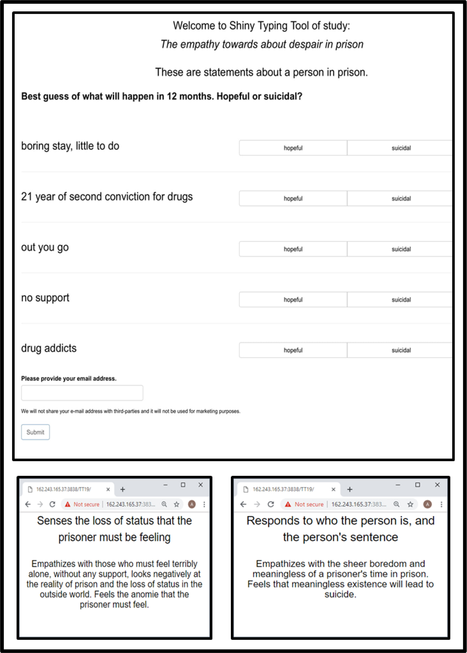
The empirical portion of this paper will show how experiential learning and critical thinking may be at the fingertips, with the use of simple computer programs, specifically BimiLeap, freely accessible at www.BimiLeap.com.  In this paper we look at how a 14-year-old student can learn about laws and ethics, as well as the issues of daily life. The topic is taken from the way young students in a Yeshiva, a rabbinic school, can learn about the issues underlying property, specifically borrowing property and what happens when the property is somehow ‘lost.’

Experiential learning and discovery of the new

A proposed approach based upon the emerging science of Mind Genomics.  Mind Genomics is an emerging science combining experimental psychology, consumer research, experimental design, and statistical modeling. The objective is to explore decision making in the everyday world.

In terms of commercial and social practice, Mind Genomics has been applied in by author HRM to issues as varied as it applies to topics as different as decision making about what we choose to eat, legal cases, and communications in medicine to improve the outcomes during and after hospitalization, respectively. These practical applications along with the ongoing stream of studies suggest Mind Genomics as a simple-to-use but powerful knowledge-creation tool. With Mind Genomics, virtually anyone can become a researcher, explore the world, classify the strategies of decision making, and discover new-to-the-world mind-sets, groups of people who think about the topic in the same way, and who differ from other groups of people thinking about the topic in a different way.

The Mind-Genomics technology has been embedded in easy-to-use computer programs, making the typical Mind Genomics study fast, affordable, and structured. The same simplicity of research, studying what is, may thus find application to educate the non-researcher, the novice, the younger student. Rather than the researcher exploring a topic area with the point of view of a person interested in the specific topic, the notion emerged that the same tool can be used to each a novice how to think, using research as a the tool, and the information and accomplishment as the reward for using the tool.

The Yeshiva approach: Havrutas (groups) studying a topic in depth

This paper presents one of the early attempts to use Mind Genomics to teach legal reasoning to a teenager, helping the teenager to make a specific topic ‘come alive’ as well as imbue experiential learning and critical thinking into the process.  The paper will present the approach step by step, as a ‘vade mecum’ or ‘guide’ for the interested reader.

The objective of Mind Genomics is to understand the decision making in a situation.  The deliverable is a simple table, which one can adorn in different ways, but which at its heart shows questions and answers about a situation.

We take our approach from the way students in Jewish religious schools study the corpus of Jewish law, commentary and discussion.  The notion of using the Bible as a source for teaching modern concepts is not new [3]. created a course on economics, based upon biblical tests, as described in the following paragraph

The author describes a course designed to build the critical thinking skills of undergraduate economics students. The course introduces and uses game theory to study the Bible. Students gain experience using game theory to formalize events and, by drawing parallels between the Bible and common economic concepts, illustrate the pervasiveness of game-theoretic reasoning across topics within economics as well as various fields of study.

We take our source for the course in the way the Talmud is study. The Talmud comprises more than 2700 of pages of explication of basic Jew practice.  The origins of the Talmud are, according to Jewish sources, founded in the Oral Law, the law of Jewish practice based in the Old Testament, the Jewish Bible, but expanded considerably.  For the reader, the important thing to know is that the Talmud comprises two portions, the Mishna, a short, accessible compilation of Jewish Law and practice, finalized by Rabbi Judah the Prince around the second century CE, and then discussions of that compilations, attempting to find discrepancies to reconcile them, done by Rabbis and their students for about 300–400 years hundred years after the Mishna was finished. This section, discussion and reconciliation among sources, is embodied in difficult, occasionally tortuous material known as the Gemara, the word in Aramaic for‘completing.’

Talmud students who spend years learning the Talmud end up thinking critically [4]. The method is to pair off students with each other, havrutas, usually comprising two students, who read, decipher, debate, and struggle to understand the section together. The approach leads, when successful, to logical thinking, and ability to formulate problems ina way worthy of a lawyer.  In the words of [5].

when examined closely, havruta study is a complex interaction which includes steps, moves, norms and identifiable modes of interpretative discussion [5].

Havruta learning or paired study is a traditional mode of Jewish text study. The term itself captures two simultaneous learning activities in which the Havruta partners engage: the study of a text and learning with a partner. Confined in the past to traditional yeshivot and limited to the study of Talmud, Havruta learning has recently made its way into a variety of professional and lay learning contexts that reflect new social realities in the world of Jewish learning [6].

With this very short introduction, the notion emerged from a number of discussions with psychology researchers and with students of the Talmud that perhaps one might use technology inspired by Talmudic style thinking and discussion to teach students to think critically, whether these be Talmud students embedded in the Jewish tradition, or students who could take a topic of the Talmud in an ‘edited’ form, and work with that topic in the way a yeshivastudent might.

Adapting the approach, making it accessible, challenging, interactive, and fun

The situation for this study is simple, based upon a legal case well known to many students of the Talmud, but presented in secular terms. The case concerns an item, the nature of which is unstated but the implication is that the item is something portable.  The information available is:

1. Who initiated the interaction?
2. Why was the interaction initiated?
3. Where was the interactioninitiated (viz., request made)?
4. What happened to the item?

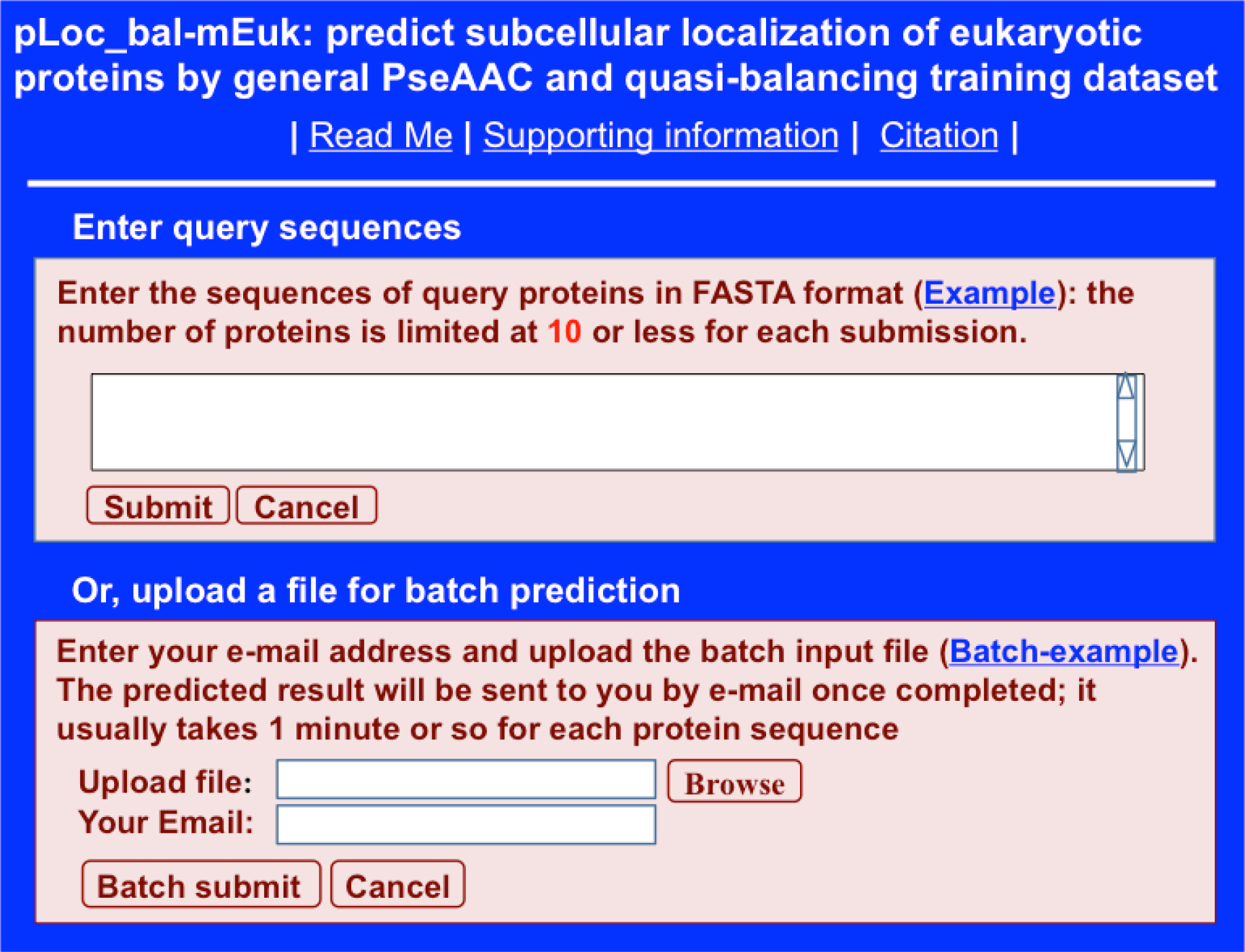
In order to make the system easy, but keep the tone serious, the design for the computer interface was created to be simple. 

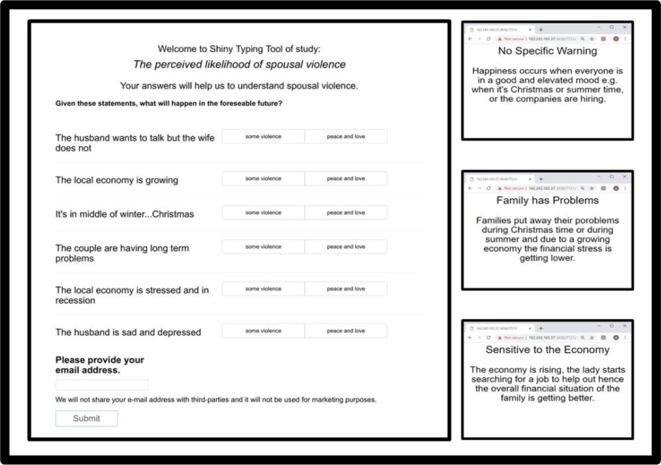
Figure 1 shows the three key screen shots.

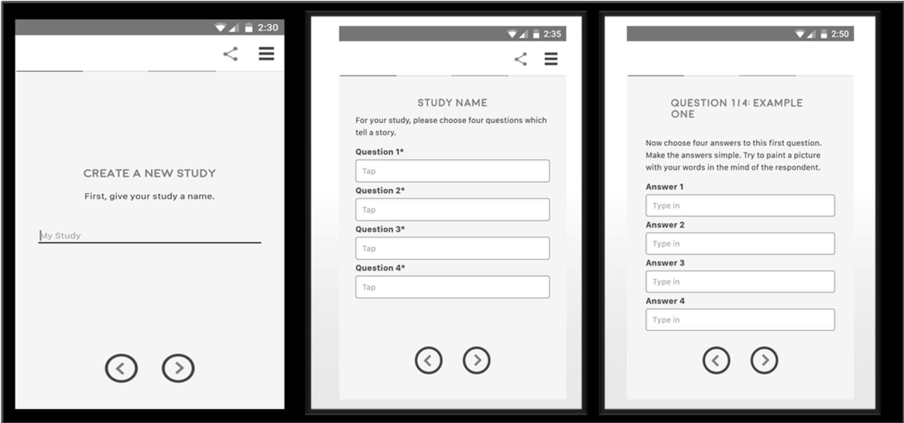
Figure 1. The setup showing the three panels which force the student to think in an analytic yet creative and participatory fashion

The left panel shows the requirement that the student(s) select a name for the study. It may seem simple, but it will be the name of the study which drives much of the thinking.

The middle panel shows the requirement to create four questions dealing with the topic, with the questions ‘telling a story.’ It is here, at this second stage, beyond the name of the topic, where students encounter problems, and must ‘rewire’ their thinking. Students are taught to understand, to remember, to regurgitate. Students are not taught to ask a series of questions to elucidate a topic.  Eventually, the students will learn how to ask these questions, but it will be much later, when the student is introduced to research in the upper grades, and when the student becomes a professional, especially a lawyer.  We are creating the opportunity to bring that disciplined thinking to the junior high school or even to grade school.

The right panel shows the requirement to provide four answers to one of the questions. There is no hint, no guidance, about what the answers should be, but simply the question repeated to guide the student.  Typically, this third panel is easy to complete once the student has gone through the pain of thinking through the four questions. That is, the questions are hard to formulate; the answers are easy to come by after the hard thinking has been done.

Engaging the student in the creation of questions and answers

The key to the approach is the set of questions, and secondarily the set of answers. As noted above, the demand on the participant is to conceptualize the topic at the start, rather than being trained to deconstruct the topic when it is fully presented.  The approach thus is synthetic, requiring imagination on the part of the student. 

Table 2 presents the four questions and the four answers to each question.  The questions and the answers do not emerge simply from the mind of the student, at least not at first. There are the inevitable false steps, the recognition that that the questions do not make sense, do not tell a story, do not flow to create a sequence, etc.  These false steps are not problems, but rather part of the back and forth learning how to reason, how to tell a coherent story, and how to discard false leads.

Table 2. The four questions, and the four answers to each question

The answers in Table 2 are simple phrases, with the introduction to the answer being a phrase to reinforce the story.  Various efforts at making the approach simply continue to reveal that for those who are beginning a topic, it is helpful to consider the answers as continuations of the questions. That specification, such as ‘initiated by’ will also make the respondent’s effort easier.

It is important to keep in mind that the process of topic/question/answer will become smoother with practice, the topics will become more interesting, the questions will move beyond simple recitation of the order of events, and the answers will become more like a literary sentence, and less like a menu item.

In the various experiences with this system, it is at this point, the four questions, that most people have difficulties. Indeed, even with practice, people find it hard to organize their thinking to bring a problem into sufficiently clear focus that they can make it into a story. When the researcher finally ‘understands the task’ the response is often a statement about ow they feel their ‘brains have been rewired.’ Never before did the researcher have to think in such a structured, analytic way, yet with no guidance about ‘what is right.’

One of the more frequent questions asked at this point is ‘Did I do this right?’  Most people are unaccustomed to structured thinking.  After creating the questions, and on the second or third effort, after the first experiment, the researcher begins to feel more comfortable, and is able to move around the order of questions, changing them to make more sense. This flexibility occurs only after the researcher feels comfortable with the process.

Creating ‘meaningful’ stimuli by means of an underlying experimental design

As students, we are typically taught the ‘scientific method,’ namely to isolate a variable, and understand it.  Our mind is attuned to dissecting a situation, focusing on one aspect.  We lose sight of the fact that the real world comprises mixtures, and that an understanding of the real world requires us to deal with the way mixtures behave.  An observation of our daily actions quickly reveals that virtually all of the situations in which we mind ourselves comprises many variables, acting simultaneously.  Indeed, much of the problem of learners is their experienced difficulties in organizing the multi-modal stimuli impinging on themand learning to focus and to prioritize.  It is to this skill we now turn as we look at the student experience.

The computer program combines alternative answers to these four questions, creating short vignettes, presents them to respondents, gets a rating of ‘must repay’ vs ‘does not need to repay’.’

The above-mentioned approach seems, at first glance, to be dry, almost overly academic. Yet, the Mind Genomics approach makes the ‘case’ into something that the students themselves can create, investigated, and report, with a PowerPoint® presentation of the study, something that will be part of their portfolio for life, and can be replicated on many different topics.

Each respondent evaluates a unique set of vignettes, created by a systematic permutation of the combinations. The mathematical rigor of the underlying experimental design is maintained, but the different combinations ensure that across all the respondents a wide number of potential combinations are evaluated.

The underlying experimental design and indeed all of the mathematics for the analysis are shielded from the respondent, who is forced to ‘think’ about the topic, and the meaning of the data, rather than getting lost in deep statistics. 

The composition of the vignettes is strictly determined by an underlying specification known as an experimental design [7]. Each vignette comprises either two, or three or four answers, at most one answer from a question, but sometimes no answer from a question.  The experimental design ensures that the 16 elements appear as statistically ‘independent of each other,’ so knowing that one answer appears in a vignette does not automatically tell us whether another answer will appear or not appear.

Figure 2 shows an example of a vignette created according to the underlying design.  The respondent does not know that the computer has systematically varied the combinations.The vignette is created by an underlying experimental design which prescribes the composition of each vignette.  Each respondent evaluates 24 different vignettes, or combinations of answers, and answers only. No questions leading to the answers are presented directly, although for this case the question is embodied at the beginning of the answer.

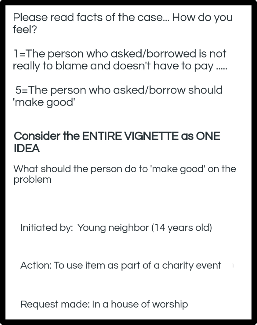
Figure 2. Example of a vignette comprising three answers or elements, one answer from three of the four questions. Most vignettes comprise four answers, some comprise three answers, and a few comprise two answers.

An important challenge in Mind Genomics is to come up with a meaningful rating question. The rating question links the test stimuli, our vignettes, and the mind of the respondent.  Without a meaningful test question all we have are a set of combinations of messages.  The test question focuses the respondent’s mind on how to interpret the information in the vignette.

The test question is posed simply as either a unipolar scale (none vs a lot) or a bipolar scale (strong on one dimension vs strong on the opposite dimension, such as hate/love).  To the degree that the researcher can make the rating question meaningful, the researcher will have added to the power of the Mind Genomics exercise.

Our topic here concerns the loss of property occasioned by one person giving property to another person, after being asked to do so, or after being motivated to do so, that motivation coming from within.  A reasonable rating question is whether the person in whom the property is placed, for whatever reason, is required to ‘make good byreplacing the property’ or ‘not required to replace the property.’  Rather than requiring a yes/no answer, we allow the respondent to assign a graded value, using a Likert Scale:

1  =   The person who asked/borrow is not really to blame and doesn’t
          have to pay ….

5  =   The person who asked/borrowed should ‘make good.’

The phrasing of the question and the simple 5-point rating scale make the evaluation easy, and remove the stress from the respondent. By allowing the student a chance to assign a graded rating, the student can begin to understand gradations of guilt and innocence. Furthermore, the answers are not so clear cut, so straightforward that they prevent the student from thinking.  The requirement to take the facts of the case into account and rate the feeling of guilt vs innocence on a graded scale forces the student to think.  The very ‘ordinariness’ of the case encourages the student to become engaged, since the case is something that no doubt the student has either experienced personally, or at least has heard about at one or another time.

Obtaining additional information from the respondent

Quite often, those who teach do not pay much attention to WHO the respondent actually is, or even the different ways that people think. The academies where the Talmud was created did pay attention to the way people think, coming up with different opinion about the same topic. These different opinions were enshrined in discussions. The intellectual growth coming from thinking about the problem was maintained over the millennium and a half through the discussions of students about different points of a topic, and the study of those who commented on the law, and gave legal opinions about cases. The back and forth discussions about why the same ‘facts on the ground’ would lead to different opinions became a wonderful intellectual springboard for better thinking.  Few people, however, went beyond that to think, in a structured way about how ordinary people might think of the problem, people who were not trained as legal scholars, nor empaneled in a judicial panel.

Part of the effort of the Mind Genomics project is to show to the student the way different people think about the topic, and how there is not necessarily ‘one right answer.’  Thus, at the start of the experiment, before the evaluation of the 24 vignettes by the respondent, the respondent is asked three questions:

1. Year of birth, to establish age
2. Gender
3. A third question, chosen by the researcher. Here is the third question for this study.

How do you feel about mistakes that are made in everyday life, by ‘accident’

1=I believe that the law is the law 2=I believe in being lenient 3=I want to know the facts of the case more

Running the study for educational purpose – Mechanics

During the past several decades, and as the Mind Genomics technology evolved and was refined, a key stumbling point, i.e., a ‘friction point’ in today’s language, continued to emerge. This was the deployment of the study in a way that could be quick, inexpensive, and thus have an effect within a short time. Two decades ago as the Internet was being developed, a great deal of the effort of a Mind Genomics study was expended getting the respondents to participate, typically by having them come into a central location, such as a shopping mall, and spending ten or 15 minutes.  The result was slow, and the pace was such that it would not serve the purposes of education. The process was slow, tedious, expensive, and not at all exciting to anyone but a serious researcher.

During the formative years of the technology, 2010–2015, efforts were put against making the system fast, with very fast feedback.  The upshot was that a study could be set up in 30 minutes or faster and deployed on the internet with simply a credit card to pay for the cost of respondents, usually about 3.00$ per respondent for what turned out to be a 4 minute study.  A field service, specializing in on-line ‘recruiting’ would provide the appropriate respondents, sending them to the link, and obtaining their completed, and motivated answers. The respondent motivation was there because they were part of the panel.

The mechanics were such that the entire study in the field would come back in less than one hour and one minute. The total analysis, including the preparation of the report in PowerPoint(r), ready for the student presentation, took less than one minute from the end of the field.  Figure 3 shows an example of the PowerPoint(r), expanded to the slide sort format, showing the systematic presentation of the results.

Figure 3. Example of the PowerPoint^® report for the study, shown inlide-sort format. The respondent receives the PowerPoint^® report and the accompany Excel^® data sheet one minute after the end of the data acquisition.The report is in color, and ‘editable.’

1. The title page, showing the study name, the researcher, the date
2. Information about the BimiLeap vision
3. The raw material – elements, rating question
4. How the data are analyzed, showing the transformation from a rating scale to a binary rating, as well as introducing the concept of ‘regression modeling’ …. This explanatory information is presented in a short, simplistic manner, yet sufficient to show the nature of mathematical (STEM) thinking
5. Tables of data showing the results from the total panel, key subgroups
6. Mind Sets – a short introduction to how people can think differently about the topic, and a short introduction to the calculations. Once again, the focus is on the findings, not on the method
7. Results from dividing the respondents into two mind-sets and three mind-sets
8. IDT – Index of Divergent Thought – showing how many elements have strong positive coefficients,   when the data are considered in terms of total panel, two mind-sets and three mind-sets, respectively. The IDT can be used to understand how well the researcher has ‘dived in’ to the topic, to uncover different ways of thinking about the topic. The IDT can be used to ‘gamify’ the research process, by providing an operationally defined, objective measure, of ‘winning ideas.’
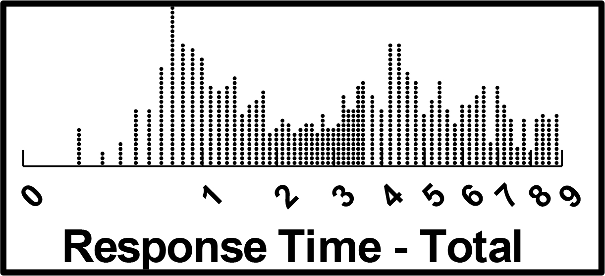
9. Introduction to ‘response time’ – how long it takes the respondent to ‘process’ the ideas
10. Tables of data showing the results from the total panel, key subgroups, and mind-sets
11. Screen shots of the respondent experience

The report is accompanied by an Excel book with the data, set up for further analysis, if the student wishes.

The results, embedded in a pre-formatted PowerPoint® presentation, and with supporting full data in Excel®, are immediately dispatched by email and can always be retrieved from the researcher’s account, when, for example, the data are ‘updated’ with the ratings assigned by new panel participants. This process compresses the entire time, from set-up to data reporting, so that the results can be discussed within 1–3 hours after the official start the entire process, viz., entering the questions and answers into the BimiLeap programming and getting the panel provider to provide respondents.

The vision behind the PowerPoint® report is that it provides a tangible record of the student’s effort, a measure of what the student has achieved in the growth to learning.  By creating different groups of students who work together, and working together for 90 minutes in the afternoon, once per week, the typical student can generate 20–30 or so PowerPoint® in a year, a collection the quality of whose contents, study by study, will demonstrably improve as each study is designed, and executed with real people, the respondents.

What the student receives and how the student learns

Table 3 presents the unadorned results, a table.  To interpret the table is straightforward, despite the fact that it has simply numbers.  The researcher who is doing the study need not know the mechanics of how the numbers are computed, at least not in the beginning, in order to enjoy the benefits of Mind Genomics, and in order to participate in experiential learning.

Table 3. Output from a Mind Genomics on a simple legal case. The data is from the total panel

The question what is the initiator (Question A) required to do.  At the low end, the initiator does not have to ‘make good’ (innocent, i.e., not pay.)  At the top end, the initiator has ‘make’ good (guilty, i.e., pay.)

Base Size: The table shows us that there are 30 different people who participated in the study. This is the base size.

Additive Constant: This is the expected number of times out of 100 people that the verdict will be ‘guilty’, i.e., must repay. What is special is that the additive constant is a baseline, corresponding to the likelihood that a person will say ‘guilty’ even in the absence of information. Our additive constant is 60. It means that when someone requests from another to do something with the item, 3 out of 5 (60%) the onus is on the person who does the requesting to take responsibility and pay if something happens to the item.

Coefficient: Ability of Each Element to drive Guilty (must repay). Let’s look at the power of Question A: Who initiated.  The four answers or alternatives, which appeared in the vignette, are either 0 (nothing) or negative. The negative means that when we know who initiated, we are likely to forgive. We forgive most when the action is initiated by a young neighbor or, or school friend in high school. The value is -10. That value -10 means the likelihood of guilty (must make good) goes from 60 (no information about the initiator) to 50, when the one piece of information about the initiator is presented as part of the case (specifically,  initiated by: School friend in high school.)  Of course, when the initiator is an older neighbor (29 years old), the coefficient is no longer -10 as it was before, but now 0. We (and of the course the student) have just discovered that it makes a difference WHO the initiator is. 

The same thinking can be done for the other questions and answers. Some, like D2 (What eventually happened: It was destroyed in accident) increase the likelihood of being judged responsible, and forced to make good, i.e., to repay.

The process from the vantage point of the researcher (e.g., the student)

As presented above, the process is simple, although quite uninteresting, except perhaps to the subject matter expert interested in lawor in thinking processes. How can the student be engaged to participate?  Otherwise, what we have here is simply another ‘dry process’ with some interesting but unexciting results.

The three aspects of the process are involvement, ease, and fast/clear results.  Absent those, and the process will remain in the domain of the expert, to be used occasionally when relevant, and otherwise to be relegated to process. The excitement of thinking and learning will not be experienced.

Let us proceed with the process.  The process follows a series of steps designed to make the researcher think. The process is structured, not particular hard after the first few experienced, but sufficiently challenging at the start so that the researcher realizes the intellectual growth which is taking place at the time of the research set up.

Experimental Designs – mixtures of answers

The actual test stimuli comprise mixtures of answer, without the questions. One can go to Table 2, and randomly pick out one answer from each of the four questions, present these answers together, on separate lines, and instruct the respondent to read the vignette, the combination, and rate the combination as a single entity.  The task may seem ‘strange’ to those who are accustomed to reading properly constructed paragraphs in their native language, but to those who are selected from random individuals to be study participants, there is no problem whatsoever. People follow instructions.   The problem with evaluating a few unconnected combinations is that there are no explicit patterns waiting to be discovery, and a discovery in turn which can teach systematic and critical thinking.

As noted above several times, the Mind Genomics paradigms works with an explicitly developed experimental design, which makes it easy for the equipped research to discover the pattern. Table 4 shows an example of the experimental design for a single respondent. There is a total of 16 answers and 24 vignettes, or combinations. The number and arrangement of the vignettes are not accidental, nor haphazard, and certainly not random, although it is tempting to say that the combinations are randomly arranged. Nothing could be further from the truth. The design, i.e., the combinations are precisely defined ahead of time , so that each of the 16 elements or answers appears exactly five time, that any vignette of combination has at most four answers (without their questions), that some combinations comprises two, others comprise three answers, and that the answers are systematically varied.  Finally, each of the experimental design is mathematically identical to every other design, but the specific combinations are different.

Table 4. The experimental design for 7 of the 24 vignettes for a respondent, as well as the rating, the binary expansion of the rating, and the consideration time

Different points of view for the same argument – Mind-Sets and exciting discoveries

Students who ask questions to engage discussion are generally appreciated by their teachers. The questions show involvement.  Sometimes the questions spark lively discussions, especially when they are offered in the spirit of ‘looking at the problem in different ways.’

A foundation stone of Mind Genomics is the recognition and elicitation of different points of view about the same topic. The ingoing rationale is that in matters of everyday life there are facts, but often radically different opinions. Sometimes more learning emerges from the discussion of the topic from these different viewpoints than could ever emerge from rote learning of the ‘facts.’

One of the computations of Mind Genomics is the discovery of different mind-sets, groups of people with these individuals in one group looking at the topic differently from individuals in another group. The computational machinery of Mind Genomics enables these mind-sets to be discovered rapidly and inserted into the PowerPoint® report as simply new groups to consider and to discuss.

Table 5 shows the additive constant and coefficients for total (already discussed), gender, age, and two mind-sets. The students who participate in the study, indeed those who may have come up with the elements, can now see how the simplest of facts can be interpreted in different ways.

Table 5. The pattern of coefficients for ‘make good’, generated by key demographic groups (total, gender, age) and newly uncovered mind-sets.

What should emerge from Table 5 is the charge to the students to ‘tell a story about the mind of each group,’ about whether the mind of the group seems to hold strong views or weak views about what makes a person guilty.  There is no right nor wrong answer, but simply the requirement that the student abstract from these data some narrative of how the group thinks.  The difference in coefficient is most dramatic for the two mind-sets, but what is the MEANING of the difference?  In that short question lies a great deal of opportunity for the students to think creatively, to see patterns, and indeed perhaps even to make new-to-the-world discoveries.  Furthermore, the excitement can be maintained by challenges to the students to create personas of the mind-sets, and to suggest and executed follow-up experiments with Mind Genomics to explore hypotheses about these mind-sets.

Learning to think even more deeply – Is justice blind, and how can the student prove or disprove it?

We finish off the data section by a new way of thinking, and two exercises can be done manually with available statistical programs, planned to be programmed into the next generation of the Mind Genomics report.  These are called ‘scenario analyses.’ The logic behind them is simple. The thinking emerging from them is far from simplistic, however. The struggle to understand the new patterns from this level of analysis helps to move the motivated student into a more profound way of thinking, in a subtle, easy, virtually painless way.

When people look at the ‘facts of the case’ they are often cautioned not to pay attention to the nature of the individuals, but simply the ‘facts on the ground,’ on what happened.  Such caution is easy to givebut may or may not be followed.   One of the opportunities afforded to the student of Mind Genomics is to understand clearly the interaction between WHO the person IS in the case, and the response.  For example, in our case we have four people who initiate the request, ranging from a young neighbor, an old neighbor, the uncle, school friend in high school.

We can learn a lot by sorting the data into five different strata, depending upon who does the requesting, and ten building the model. We don’t know what exactly happened to the item, but we do know who did the requesting.  We build the model based upon the five strata. Each stratum corresponds to one person who requested.  The independent variables are the three other aspects (action: where request was made; what happened.).

The original set up of the Mind Genomics process was to create four questions, and for each question develop four answers.  As described above, the underlying experimental design mixed and matched the combinations according to a plan. Each respondent, i.e., test participant, evaluated 24 different vignettes. Furthermore, unknown to the respondents, an underlying system created different sets of 24 vignettes, a unique set of combinations for each respondent.

It makes no difference to the respondent about the way the combinations are created. Whether the same 24 combinations are tested by 30 different people (the ordinary way), or whether the systemic variation produces 720 different combinations (24 different combinations x 30 different people), is irrelevant to the individual respondent. What happens, however, to the judgments when we look at five different groups of vignettes, varying, say, by WHO DOES THE INITIATION.  We have vignettes with no mention of who does the initiation, as well as vignettes specifying the initiation by the younger neighbor (14 years old), the older neighbor (29 years old), by a school friend in high school, and by the person uncle.

The question which emerges, one provoking a great of discussion, is whether justice is blind.  That is, the intended actions can be the same, the place where the request was made can be the same, and the outcome can be the same. Presumably, it does not matter WHO initiates the request. Justice should be blind. Is it?

We can sort the data into five strata, five groups, with each group comprising one of the five alternatives of ‘initiated by.’  There are five groups or strata because on group has NO mentionof ‘Initiated by:’ The next step is to estimate the coefficients, this time using only the remaining 12 elements. A1-A4 are absent from the regression because the regression is done on a stratum-by-stratum basis, where the element ‘Initiated by:’ is held constant.

After this effort the excitement increases when the students realize how strongly the initiator ‘drives’ the rating of ‘make good’ (i.e., rating of 4–5 converted to 100.)  Table 6 shows this analysis when the strata are based upon Question A (Who Initiated?). Table 7 shows the comparable analysis when the strata are based upon Question B (Action or Purpose).  In both cases there is plenty of space for discovery and for an ah ha experience, as the student uncovers truly new findings, itself motivating, and struggles to explain what she or he has revealed to the world.

Table 6. Coefficients for the models relating presence/absence of elements to the binary transformed rating ‘make good’ (i.e., guilty). The table shows the contribution of each of the elements to ‘make good’ when the ‘Initiated by’ was constant.

Table 7. Coefficients for the models relating presence/absence of elements to the binary transformed rating ‘make good’ (i.e., guilty). The table shows the contribution of each of the elements to ‘make good’ when the ‘Action’ or purpose was constant.

IDT – Index of Divergent Thinking: Making the Mind Genomics into a game

As of this writing (early 2020), the world of students is awash with games, with fun, with a shortened attention span, and with the competition of different forms of entertainment. How do we convert Mind Genomics to entertainment or at least to that over-used neologism ‘edu-tainment?’

The notion of converting critical thinking to ‘games’ requires that there be criteria on which people can complete, and that these criteria be objective, rather than subjective.  That is, to make Mind Genomics into a ‘game’ with points means to create an easy-to-understand scoring system, and specifically a system within which everyone can compete.  Furthermore, in the spirit of critical thinking and experiential learning, the system should reward creative thought.

During the past three years author H Moskowitz has worked on criteria to ‘measure’ critical and creative thought within the framework of Mind Genomics. A key aspect of Mind Genomics is that it automatically estimates the degree of linkage between each of the 16 elements and the rating scale, after the rating is converted to a binary score, 0 or 100.  This linkage is the coefficient from the model relating the presence/absence of the elements to the binary transformed rating.  It will be the linkage, the coefficient, which provides the necessary data to create a gaming aspect to the Mind Genomics exercise.

Consider the tabulation of coefficients in Table 8. Table 8 presents the distribution of POSITIVE coefficients for six different groups which always appear in the Mind Genomics reports. The six groups are total panel, Mind Sets 1 and 2 from the two Mind-Set solutions, and then Mind Sets 1, 2 and 3 from the three Mind-Set solution.  We saw the total panel and the results from the two mind-sets, but not from the three mind-sets.

We tabulate the frequencies of coefficients between 0 and 5, 5 and 10, 10 and 15, 15 and 20, and finally higher than 20.  This tabulation generates a distribution of coefficients. We can either work with the absolute number of coefficients of a certain size (Computation 1) or weight the number of coefficients by the relative size of the subgroupsshowing the particular magnitude of coefficients (Computation 2.)

The summaries in Table 8 provide a quantitative, objective measure of ‘how good the elements are’ as they drive the response. When a student produces elements that score well across the different mind-sets, this is evidence of good thinking on the part of the study, thinking which is sufficiently powerful and expansive as to appeal to different-minded groups,

Table 8. Computation for the IDT, Index of Divergent Thought, a prospective gamifying metric to make Mind Genomics more interesting by being ‘gamified.’

A one-year educational plan for Mind-Genomics to develop the student mind

1. Goal: A one-year plan to create massive intellectual development among students through a once/week exercise using Mind Genomics through the BimiLeap program. The outcome… for each person, an individual portfolio of 20–30 studies showing topics investigated by the student … a portfolio to be shown proudly at interviews, and in school to be shared with fellow students, creating a virtuous circle of learning & knowledge
2. The benefit to the education system: Create a school system which produces first rate creative thinking in younger students ages 7–13, high school students, and university students, each developing far beyond who they are today. Use the BiMiLeap program in the classroom or after school, once/week, to do a study in a topic area of intellectual interest, making it a social process which combines learning, true discovery, and competition,
3. Process:  Four students work together. The younger students work with an older ‘docent.’ The docent records the material, prepares input for BimiLeap, ensures that the input is correctly submitted to the APP, and reviews the automated report with the students in the group after the data are obtained.  Each week, the composition of the group changes, allowing different students to collaborate.
4. Mechanics:  The actual mechanics of the approach are presented in this paper. Mind Genomics studies concern a single topic area and collects data by obtaining reactions through an experiment, albeit an experiment which looks like a survey, but is not. Each group will get a topic from school, create the materials, run the study, get the PowerPoint® report, discuss, add insights to the PowerPoint,  present it in class to the other groups, incorporate the report into one’s personalized portfolio, and then repeat the process the following week with a reconstituted group.
5. Specifics – Number of topics:  We believe that one good policy is to select a set of 10 topic areas, so each topic is treated 2–3 times a year by the students. Each time, the group addresses one of the topics afresh, encouraged to think critically about it and not just accept or replicate prior knowledge. They are freed to create new knowledge on the topic by re-using, updating, or adding new content.
6. Specifics – The ‘sweet spot’ for users: The older students focus on different aspects of a single general topic, with each student creating 8–12 reports on research about the mind of people responding to different aspects of the topic …  Worthy of a PhD at the age of say 15, all while having fun, learning to think, collaborate, present.
7. The BimiLeap program can be found at www.BimiLeap.com

References

1. Kahneman D (2011) Thinking, Fast and Slow. Macmillan.
2. Moskowitz HR, Gofman A, Beckley J, Ashman H (2006) Founding a new science: Mind genomics. Journal of sensory studies 2: 266–307.
3. Mc Cannon BC (2007) Using game theory and the Bible to build critical thinking skills. The Journal of Economic Education 38: 160–164.
4. Lehman M, Kanarek J (2011) Talmud: Making a case for Talmud pedagogy—the Talmud as an educational model. In International Handbook of Jewish Education, Springer, Dordrecht, 581–596.
5. Kent O (2006) Interactive text study: A case of havruta learning. Journal of Jewish Education 72: 205–232.
6. Holzer E, 7 Kent O, (2011) Havruta: What do we know and what can we hope to learn from studying in havruta? In International handbook of Jewish education, Springer, Dordrecht, 404–417.
7. Box GE, Hunter WG, Hunter JS (1978) Statistics for Experimenters, New York, John Wiley

DOI: 10.31038/PSYJ.2020213

Abstract

We present a new way to understand how people perceive situations involving other people, situations that could be considered part of the everyday. The approach is Mind Genomics, which assesses the response of people to short, systematically varied vignettes about situations and other people. The responses to these vignettes are deconstructed into the part-worth contribution of the component elements that the vignette comprises, showing the ‘algebra of the mind.’ The deconstruction also is done on response time to the vignettes, showing the ability of the elements to engage attention when the respondent makes a judgment. When Mind Genomics is applied to descriptions of family life under stress, the data suggest that some elements are linked to predicted violence, others are not. Women appear to be more sensitive than men to the individual elements. Three different mind-sets emerged with different perceived ‘triggers’ to predicted family violence, with each mind-set encompassing both men and women: Mind-Set 1 – no specific warning; Mind-Set 2 – Sensitive to the economy; Mind-Set 3 – Family has problems. We present the PVI (personal viewpoint identifier) as a technique to assign new people to these mind-sets.

Introduction

Violence against the other sex, especially in marriage, is not new. Stories of murder and abuse fill the newspapers, the magazines, and the Internet news of today (late 2019.) Before today’s overwhelming plethora of news, violence by males against females, especially spouses and other family members, occupied a great deal of attention, from those in the news, but of course even more telling, from writers and poets. One cannot read the famous poem, My Last Duchess, by the 19^th Century British poet, Robert Browning without a shudder when one realizes how easy it was to kill one’s spouse. And of course, the popular 1965 Rock n Roll song by Herman’s Hermits, hints at England’s royal lady-killer, King Henry VIII, transformed to a 1960’s idiom of a man with a broken heart.

What is popular in literature only reflects what is the common situation in everyday life. The literature in sociology and psychology is replete with studies about violence and anger. Violence against one’s spouse is dealt with in many publications, with the aspects dissected, studied, statistically analyzed and reports issued. Violence seems to be endemic to the relations, starting even in courtship [1]. The spousal violence continues, even into the 60’s [2]. Violence emerges when the woman ends up supporting the man [3]. Of course, alcoholism plays a role [4], but so does religion [5]. Violence comes from many quarters, but many studies have focused on gender and marriage [6, 7, 8].

The foregoing represents just a bit of the available material on violence in the home. These studies focus on both surveys and discussions with individuals. What is lacking is a sense of the richness of the family life through discussion, an absence promoted by the rigidity of the scientific method, but the absence filled by clinicians and social workers. The key issue is to make this topic come alive by merging the rigor of science with the immediacy of storytelling.

 Violence in the home is especially relevant because it is common and riveting to those involved. Although there seems to be very little academically oriented literature recounting the actual ‘story’ of the abuse, the Internet provides a repository of such personal studies in a number of websites, such as:

1. https://www.getdomesticviolencehelp.com/domestic-violence-stories
2. www.hiddenhurt.co.uk/domestic_violence_stories.html
3. https://www.domesticshelters.org/articles/true-survivor-stories

It may be that websites are more conducive to people ‘telling their story’ in their own language. In contrast, the scientific community has made its information almost unobtainable, except to those schooled in the scholastic tradition, and able to cut through the jargon and statistics to understand what exactly is happening

Exploratory studies through Mind Genomics

This study explores the mind of ‘people’ by having them evaluate different vignettes about violence, vignettes that have been systematically varied, with the components of the vignette, the element, having a richness that is missing from surveys

A review of the scientific literature suggests that many of the studies involving human judgment are done in a manner which is slow, expensive, requiring teams of researchers, and extensive, rigorous statistical analysis. The statistical analysis is often of the type known as ‘inferential,’ with the objective to confirm or to falsify an ingoing hypothesis, with the hypothesis developed from theory.

Mind Genomics presents to the world of science a different approach, not grounded in theory and confirming or falsifying hypotheses [9]. Rather, Mind Genomics can be liked to an exploration of decisions, using cognitively meaningful stimuli, and dealing with issues of the every day. Mind Genomics can be likened to a new cartographical exercise of a land. Mind Genomics works by presenting vignettes to the respondents, with these vignettes comprising combinations of elements or messages to which a respondent can relate. The respondent reads the vignette and responds to the combination. The research approach is analogous to the MRI, which takes multiple pictures of tissue from different vantage points, and then combines these into a picture of the tissue.

The research in this study embodies the Mind Genomics paradigm, dealing with the very important issue of family violence. The objective is to understand a third-party’s estimate of either violence or peace at home occurring when a specific situation is presented, and then to assess the likelihood that each specific element is correlated either with violence or with a peaceful home, respectively, two opposite sides of the scale.

Mind Genomics combines the person with emotion and meaningful description of behavior, i.e., cognitively rich test stimuli. Mind Genomics obtains ratings from the response of people to vignettes about a situation, similar that presented in literature, storytelling, or song. The vignette paints a picture of a situation. The respondent is then asked to judge some aspect of the situation, such as projected violence or projected happiness, based upon what is read. Through this approach it now becomes possible to understand the mind of the person, either the one who is undergoing the experience, or the one who is hearing/reading about the experience. Both points of view differ dramatically from the almost lifeless array of statistics describing a situation. Mind Genomics combines the vividness of experience with numbers, probing the inner mind of the person exposed to the situation, first-hand or second-hand.

The Mind Genomics approach

The Mind Genomics approach is designed to be exploratory, affordable, iterative, and scalable. This set of objectives in the design means that there are certain simple aspects of the study:

1. Exploratory. As suggested above, Mind Genomics does not work by confirming or disconfirming a hypothesis extant in the scientific literature. Rather, the exploration means taking new ideas from every-day experience and exploring them to find out the degree to which people respond positively or negatively to them.
2. Affordable. Mind Genomics is set up to be a so-called DIY, Do it yourself system. The researcher needs access to an APP on the proper machine (Android or Kindle), the ideas (for the researcher), and a convenient source of respondents.
3. Iterative. Mind Genomics is set up to return the data in easy-to-read formats (PowerPoint® for presentation, Excel® for data analysis. The data return in a matter of a few hours. A new study can be launched a few hours later, after the results from the first study are digested. Furthermore, the results are easy to understand, and set up to promote further exploration with the same tool. With the iterative approach the researcher can do as many as 4–6 studies in a 24-hour period, each study building upon the previous study.
4. Scalable. Almost anyone can use Mind Genomics to explore problems. The system is scalable across people, but also across different aspects of a topic, by the same researcher. Within a matter of a week or two, the enterprising researcher can conduct 10–20 studies, exploring the different facets of a topic.

Raw materials

The origin of this study was the focus by author Peer on the causes of violence against women, the fact that so much is known, yet so little. When random people were asked by author Moskowitz about the topic ‘What do you think causes spousal violence,’ very few people could provide an answer quickly. There was no sense of a well-recognized phenomenon, violence, connected with the daily life of people, other than general statistical compilations, available in the literature.

The benefit of a Mind Genomics study is the degree to which it takes any topic and reduces that topic to a set of common aspects, experienced in the everyday. Thus, the elements shown in Table 1 represent the way a person might conceive of the nature of spousal violence. A Mind Genomics is not meant to be exhaustive, but rather introductory, approachable, and in some ways focuses on a very specific topic. When this notion of ‘cartography’ is recognized and accepted, the position of Mind Genomics advances to a useful, early-stage way of understanding a topic from the mind of people.

Table 1. The raw materials for the study, comprising four questions about the conditions of a family, and the four answers to each question.

The reader will see the approach in Table 1, showing the four questions (which tell a story), and the four answers to each question. As we read the answers or elements, we should keep in mind that the answers are concrete and simple. When exploring a topic, we can learn a great deal from four simple questions which tell a story, and from the pattern of responses to the 16 answers. The results in this study should reveal a variety of new-to-the-world patterns about domestic violence, based simply on the different ways that people respond to these unambiguous stimuli.

With the inputs shown in Table 1, Mind Genomics creates combinations of answers, so-called vignettes. An example of a vignette appears in Figure 1.

Figure 1. Example of a vignette as presented to the respondent.

Each respondent evaluated 24 vignettes. The vignettes were constructed according to an experimental design, with the property that a vignette comprised at most one answer from each question, but often had no answers from either one or two of the questions. Thus, the vignettes comprised either two, three, or four answers, the so-called elements. Furthermore, each respondent evaluated a unique set of combinations. The underlying structure of the combinations was maintained, but the specific combinations differed from one respondent to another.

To the respondent, the combinations might seem to be random, but the reality is the exact opposite. The experimental design prescribes the combinations. The objective is to present combinations of elements or answers (without the questions), obtain ratings from the respondents who evaluate these combinations, and then deconstruct the ratings into the separate contribution from each element. In this way the respondent is unable to ‘game’ the system by providing politically correct answers. It is virtually impossible to detect the underlying pattern. As a result, the respondent simply relaxes, and gives responses which are more intuitive, and fundamentally less ‘edited.’ In the words of experimental psychologist Daniel Kahneman, the Mind Genomics approach calls into play ‘System 1’ thinking, the fast, almost automatic thinking that we use daily in our lives, when we don’t have to make rational calculations [10].

A sense of the underlying experimental design can be gotten from looking at the schematic in Table 2, which presents the structure of the first eight vignettes for Respondent #1. The respondent does not, of course, see the underlying structure, but rather the actual combinations, presented on the computer as in Figure 1, or restructured to fit on the screen of a smartphone.

Table 2. Structure of the first eight vignettes for Respondent #1, the conversion to binary for statistical analysis, and the deconstruction of the ratings and response time.

Executing the study

Each respondent receives the invitation to participate, and is instructed to read the vignette, and to rate it on the 9-point scale.

Here is a set of snapshots of families. Please read the full snapshot and tell us what will happen within the foreseeable future. Read the whole snapshot. Is it going to be peaceful or do you sense some family violence brewing?

What will happen in the foreseeable future with this family?

1=peace and love … 9=some violence

The respondent then read each of 24 unique vignettes. The respondent rated vignette on the above 9-point scale. The respondent was then instructed to fill out an open-ended question about violence (results not presented here.) The entire process took approximately 4–5 minutes.

Basic data transformation

The experimental design itself must be transformed to a binary no/yes, as shown in Table 2. Only with a binary scale (absent/present) is it feasible to understand the part-worth contribution of every element. In turn, the 9-point scale can be used as a dependent variable, but experience has shown that most people, researchers included, have a difficult time understanding what the scale points mean. Sometimes this difficulty in understand is addressed by labelling each of the nine scale points, a task which itself is fraught with difficulties. An easier way, taken from the world of consumer research, converts the nine-point scale to a binary scale, 0 or 100. Managers find it easy to understand the binary scale and know what to do with a ‘no’ or a ‘yes’ answer.

The conventional way to divide the scale creates three regions for the scale; 1–3, 4–6, and 7–9, respectively. Then the following conventions is invoked:

Ratings of 7–9 are assumed to represent ‘violence,’ and ratings 1–6 are assumed to reflect the lack of violence. For this new variable, ‘violence’, we convert ratings of 1–6 to 0, and ratings of 7–9 to 100. We then add a small random number (<10^–5). The small random number ensures that that the regression analysis will ‘run’ on the binary-transformed data, even when the respondent confines all of the ratings either to the lower portion of the scale (1–6, transformed to 0), or confines all of the ratings to the upper portion of the scale (7–9 transformed to 100, 1–6 transformed to 0). The small random number provides just enough variability in the dependent to ensure that the OLS (ordinary least=squares) regression ‘does not crash,’

Analysis – What drives violence versus happiness – total panel?

The basic analysis in Mind Genomics is OLS (ordinary least-squares) regression, made possible by the ingoing structure of the vignettes for each individual respondent. Every respondent evaluated 24 carefully constructed vignettes, ensuring that at the individual level all 16 elements or answers to the questions, are statistically independent of each other. Most of the vignettes are different from each other, so that the combination of all the vignettes covers a great deal of the ‘design space.’

We combine all the data from the 50 respondents, creating a database of 1200 vignettes (50 × 24 = 1200). We run two OLS regressions. The first relates the presence/absence of all 16 variables to the binary value of ‘violence’, corresponding to the ratings 7–9 on the original 9-point scale, but now becoming the value 100 on the binary scale for violence. The second OLS regression relates the presence/absence of all 16 variables to the violence of ‘happiness’ corresponding to the ratings of 1–3 on the original 9-point scale.

Table 3 shows the coefficients for the two equations. The equation is expressed as (Binary Rating) = k₀ + k₁(A1) + k₂(A2) + … k₁₆(D4).

Table 3. Parameters of the model for the Total Panel relating the presence / absence of the 16 elements to predicted violence (Ratings of 7–9 converted to 100), and to predicted happiness (Ratings of 1–3 converted to 100).

The additive constant, k₀, is the estimated value of the binary response in the absence of elements. All vignettes comprised a minimum of two and a maximum of four elements. Consequently, the additive constant is an estimated parameter. Nonetheless, the additive constant has value in because it gives a sense of baseline interest or baseline feeling, in the absence of elements.

As noted above, the experimental designs ensure that all 16 elements or answers are statistically independent of each other, allowing the absolute coefficients to be estimated. That is, the values of the coefficients are all relative to 0. A coefficient of 10 is twice as high as a coefficient of 5. Furthermore, the transformation of the scale to binary strengthens the mathematic property. The coefficient of 10 means that in the absence of elements, 10% of the responses will be suggest ‘violence’ (7–9). The coefficient of 5 means that in the absence of elements, 5% of the responses, half the number as before, will suggest ‘violence.’ The absolute value of the coefficient means that the coefficients can be compared from study to study, with different topics and different respondents. The ratio scale properties generated by the binary transformation means that one can relate ratio changes in the coefficients (or properly coefficient + additive constant) to external behaviors. The negative coefficient means that when the element is added to the vignette, the percent of response suggesting ‘violence’ will be removed. Thus, when the coefficient is -10, then adding the element to a vignette will decrease the percent suggesting ‘violence’ by 10%. The coefficients are additive and subtractive.

From thousands of such experiments, a set of rules of thumb have emerged about the value of the coefficients, based upon observations of the data, and knowledge about what happens in the external world. The table below provides these guidelines, which are qualitative in nature. There are no fixed values, but rather a shading of importance, so that the higher the positive number the more important the element.

1. Coefficient of 15 or higher             Extremely important, major signal
2. Coefficient 8–15                           Important to very important
3. Coefficient of 0–8                         From irrelevant to almost important
4. Coefficient 0 to -6                        From irrelevant to almost important
5. Coefficient from -6 to lower           Important

We interpret the parameters of the model for violence (ratings of 7–9 converted to 100).

1. The Additive constant is 27, meaning that there is a low likelihood of predicting violence in the absence of elements. We can compare this to say the purchase intent for pizza on the same type of 9-point scale, albeit with different anchors (definitely not buy … definitely buy). The additive constant for pizza is around 60.
2. The elements for predicted violence are low. There is only one which even approaches potential meaningfulness, C4 (The husband is sad and depressed).
3. We move now to the parameters of the model for happiness (ratings of 1–3 converted to 100.)
4. The additive constant is 12, meaning that there is very little in the way of predicted happiness in the absence of elements.
5. Two elements emerge as strong drivers of predicted happiness, both related to season:
   1. B4 (It’s summer time)
   2. B3 (It’s the middle of winter … Christmas)

Genders react differently when predicting violence, but similarly when predicting happiness

Respondents profiled themselves in term of gender. When we divide the data sets by gender and estimate the two models by gender (predicted violence versus predicted happiness), we find dramatic differences in the models for predicted violence, but similar models for predicted happiness (Table 4).

Table 4. Parameters of the model for males versus females relating the presence / absence of the 16 elements to predicted violence (Ratings of 7–9 converted to 100), and to predicted happiness (Ratings of 1–3 converted to 100).

Table 5. Parameters of the model for the three age groups relating the presence / absence of the 16 elements to predicted violence (Ratings of 7–9 converted to 100), and to predicted happiness (Ratings of 1–3 converted to 100).

Predicted violence

1. Additive constant – lower for females, higher for males (16 vs 39). The difference suggests that the prediction of violence by female respondent occurs for specific situations. In contrast, for males the additive constant is much higher, suggesting that they predict violence without needing to have specifics.
2. Women predict that the violence will occur in different situations, the most surprising of which is the expectation of violence during Christmas time.

   The husband is sad and depressed

   Companies are firing employees

   It’s in middle of winter … Christmas

Predicted happiness

1. Additive constant is very low, 11 for females, 13 for 13
2. Surprisingly, women are divided on winter and Christmas, with females reacting to

   It’s in the middle of winter … Christmas

   The local economy is growing

   It’s summer time

3. Males are happy as well, with both season and a growing economy

   It’s in the middle of winter … Christmas

   Companies are hiring but people are working long hours

   It’s summer time

Predicted Violence

1. The additive constants, prediction of violence without other information, are low, with the additive constant lowest for age 50+ (value = 22), and the additive constant modestly higher for age 19 to 29 (value =31)
2. There are age differences in what drives predicted violence.
3. The oldest respondents, age 50+ predict that violence will occur with the husband sad and depressed, and the companies firing employees.
4. The middle group age predict that violence will occur when the local economy is stressed and in recession
5. The young respondents don’t predict violence will occur in these bad economic times but predict violence will occur when the wife wants to talk but the husband does not.
6. We conclude from this pattern that the older respondents, age 50+, see violence as externally driven, whereas the young respondents, age 19–29 see violence as interaction driven.

Predicted happiness

1. The additive constants, base expectations without elements, vary dramatically across ages. The older respondents (age 50+ and age 30 to 49) see no basic happiness. It’s all a matter of the specifics. The younger respondents, age 19 to 29, in contrast, feel that happiness is all around.
2. The oldest respondents feel that happiness is a function of the time, whether Christmas or the summer.
3. The middle group, age 30 to 39, show some answers which make sense (e.g., companies are honoring, summer time, winter time), but also some answers which don’t make sense (companies are firing employees’ the local economy is stressed and in recession). It could be that this age group feels that the hard times will bring the couple together, rather than eventuate in violence.
4. The youngest group age 19 to 39 feel that happiness will emerge with the Christmas season, but not with the summer season.

Response time and engagement with the elements in the vignette

For more than a century, researchers have searched for ‘objective’ correlates of psychological processes. The notion that the information provided by people was not acceptable to many researchers, who believed, whether correctly or not, that only ‘objective’ physical measures could tell the truth about what a person perceives or thinks. The history of these approaches traces back to the original research on reaction time in the Leipzig laboratory of Wilhelm Wundt [11], and moves on to physiological measures of human reactions, whether GSR (galvanic skin response, electrical conductance of the skin), electromyography (muscle currents), then EEG (electroencephalographs and brain waves), culminating in such methods as fMRI [12, 13]. There are other more recently introduced methods, such as the implicit association test [14].

Response time, the earliest measure and perhaps the most frequently used measure, may shed additional light on the nature of the way people respond to the elements or answers embedded in the vignettes. Mind Genomics has the distinct benefit that the test stimuli, the elements, are themselves cognitively meaningful. It’s not a case of having to infer ‘what about the stimulus’ makes the respondent process it more quickly or more slowly. One can simply look at the response times to the different elements, using deconstruction method below, and ask whether there is something common about those elements taking longer to process, versus those elements processed more quickly.

The Mind Genomics computer program measured the response time to the different vignettes. It then eliminated all vignettes requiring more than 9 seconds to rate, under the assumption that in these Mind Genomics studies, rarely does a respondent stop to consider a vignette for longer than a few seconds. The Mind Genomics program also eliminates all vignettes tested in the first position, with the rationale that at the start of the experiment respondents don’t know what to do.

Figure 2 shows the distribution of response times, with the abscissa spaced logarithmically. The important thing is the relatively large number of vignettes requiring more than four seconds to process. In many comparable studies, albeit with mundane topics like food, we do not see such long response times. There may be a difference in the way people read serious vignettes, such as the vignettes here, versus ‘fun vignettes’ of other topics.

Figure 2. Distribution of response times for the study on predicted family violence. The distribution has been trimmed to eliminate the responses from the vignette evaluated in the first position, and vignettes registering 9 seconds or longer to evaluate.

The analysis of response times follows the standard approach, involving OLS (ordinary least-squares) regression. The equation is written without the additive constant, based upon the ingoing assumption that in the absence of a vignette with elements, there is no response. All vignettes, however, except those tested first, are included in the OLS regression, with all vignettes of response times 9 or more seconds truncated to 9.

The equation is expressed as: Response Time = k₁(A1) + k₂(A2) … k₁₆(D4)

The analysis was performed in the precisely the same way as the regression analyses for the ratings. That is, the relevant group was identified, and all the appropriate vignettes from everyone in the relevant group was put into a single data file, accessed by the OLS regression package.

The coefficients represent the number of tenths of seconds that can be ascribed to each element. The OLS regression deconstructs the response time, estimating the number of tenths of seconds for each element. In the analyses we will look at those response times for individual elements of 1.5 seconds or more. The cut-off of 1.5 seconds is arbitrary, allowing us to get a sense of those elements which strongly engaged the respondents. It is important to keep in mind that these socially relevant topics appear to be generating longer response times than the more typical business and marketing topics run in the same fashion, with the same type of respondents. It may be that respondents pay more attention to socially relevant topics.

The response times for the 16 elements as shown in Table 6 suggest a continuum with response times of 1.0–1.5 seconds. Keep in mind that all response times over 9 seconds or longer were eliminated as suggesting that the respondent might be doing other things. The data do not suggest a pattern. The most engaging elements, those with the longest response times, talk about the couple, about the economy, and about the woman having problems.

Table 6. Response times for the 16 elements, estimated from the data of the Total Panel.

By gender

When we divide the respondents by gender, we see radical differences. The most important result is that men do not find the elements engaging, at least when we operationally define the term ‘engaging’ as a response time of 1.5 seconds (Table 7.)

Table 7. Response times for the 16 elements, estimated from the data broken out by gender.

Table 7. Response times for the 16 elements, estimated from the data broken out by age group.

Males

The most engaging element is

The lady is having problems with finances.

The least engaging elements are

The wife wants to talk but the husband does not

Companies are firing employees

It’s summer time

The family time is shorter together

The husband is having job troubles

Females

There are many engaging elements. The fact that 8 of the 16 elements are engaging to women suggest that women are simply more attentive than men to the topic of violence versus happiness.

The husband wants to talk but the wife does not

The couple are having long term problems

Companies are hiring but people working long hours

The lady is having problems with finances

The local economy is stressed and in recession

The wife wants to talk but the husband does not

It’s in middle of winter … Christmas

Companies are firing employees

Age group

Respondents age 59+

The oldest respondents focus primarily about the issues between the members of the couple, but also react to the economy (companies are hiring but people working long hours). That element might be a signal for problems that emerge between the husband and wife.

Companies are hiring but people working long hours
The husband wants to talk but the wife does not
The couple are having long term problems
The wife wants to talk but the husband does not
The lady is having problems with finances
It’s in middle of winter … Christmas
Companies are firing employees
The lady starts searching for a job to help out

Respondents age 30–49

The most engaging element is the practical issue of finances. The elements are more practical.

The lady is having problems with finances
The family all eat at different times
The local economy is growing

Respondents age -29

None of the elements engaged them. They appear to be disinterested in the topic, or at least don’t pay much attention.

Mind Sets

One of the key tenets of Mind Genomics is that in any topic area involving judgment and decision-making, there are different groups, mind-sets, showing divergent patterns of what is important. The ideal situation, but one quite rare, is that these mind-sets are congruent with some easy-to-define and measure characteristic or set of characteristics of the respondent. Most of psychological and sociological research discovering groups with different points of view, e.g., voting for political parties, attempt to understand these differences within the framework of the standard ways to divide people. Thus, it is not unusual to see voting patterns broken out by age, gender, market, income, education, work, and so forth. Indeed, the world of analytics attempts to predict these mind-set-driven behaviors from some predictive model using easy to measure variables.

In the world of Mind Genomics, the discovery of these basic groups is straightforward, requiring simply one or several studies of the type performed here, and statistical methods to cluster together individuals with similar patterns of coefficients [15]. Individuals with similar patterns are assumed to belong to the same ‘mind genome’ for the topic. The creation of the mind genome is a simple statistical analysis, once the relevant experiment has been run. In this respect Mind Genomics holds the advantage of generating easy to interpret ‘mind genomes’ from simple experiments. The reason for the simplicity is that the experiment deals with the topic itself, and the test stimuli are all relevant. One need not array an analytic armory to discover the ‘mind genomes,’ which emerge readily from these focused experiments.

The procedure for uncovering mind genomes follows these eight steps.

1. Array the vector of all 16 elements for a given respondent as a one line in a data base.
2. Create all the data base, which in our case comprises 16 columns of data (one column per element), and 50 rows (one per respondent).
3. The coefficients tell us the degree to which the respondent would rate that element a 7–9 if the vignette comprised only that element.
4. Apply the method of clustering to divide the set of respondents into two groups, and then again into three groups.
5. Build a model for each of the two groups, and then build a model for each of the three groups.
6. Choose the more parsimonious solution, which is at the same time interpretable.
7. Interpretable means that the strongest positive elements ‘tell a coherent story’.
8. Parsimonious means that the fewer the number of clusters or mind-sets, the better, so long as the mind-sets tell a story which makes sense.

The results from the clustering suggest three mind-sets, as shown in Table 8. The clustering was done on the coefficients after the ratings were converted to the ‘predicted violence scale’ (ratings of 7–9 converted to 100, ratings of 1–6 converted to 0). The mind-sets are named according to the elements which generate the highest coefficients for the mind-set.

Table 8. Parameters of the model for the mind-sets relating the presence / absence of the 16 elements to predicted violence (Ratings of 7–9 converted to 100), and to predicted happiness (Ratings of 1–3 converted to 100.) The mind-sets were generated based upon the predicted violence scale.

When we look at response times for the three mind-sets (Table 9) we see dramatic differences in the pattern of elements which ‘engage,’ i.e., operationally defined as generating a response time of 1.5 seconds or longer. The elements which drive the segmentation also appear to strongly engage only respondents in Mind-Set 3 (family has problems),

Table 9. Response times for the 16 elements, estimated from the separate models, one for each of the three mind-sets.

Mind-Set 3 (Family has problems)

Companies are hiring but people working long hours
The couple are having long term problems
The lady is having problems with finances
The husband wants to talk but the wife does not
Companies are firing employees
It’s in middle of winter are Christmas

Mind-Set 2 (Sensitive to the economy)

The wife wants to talk but the husband does not
The family all eat at different times
The couple are having long term problems
The local economy is stressed and in recession
The husband wants to talk but the wife does not
The local economy is growing

Mind-Set 1 (No specific warning)

No element engages

The nature of people – optimistic versus pessimistic

The original focus of this paper was the pattern of responses of people to vignettes describing a couple who are in a stressful situation. The pattern of responses of our 50 respondents can also show us whether the respondents themselves are typically optimistic, pessimistic, or neither. The analysis is straightforward. We have 24 samples of the respondent’s evaluations of vignettes, with all elements (answers) appearing an equal number of times, and the basic experimental design structure maintained.

In our preparation for modeling we created binary two scales, each 0/100. Each respondent generates an average on each binary scale. When we look at predicted violence, for example, an average of 100 means that 100% of the time, i.e., for all 24 vignettes, the respondent predicts violence will occur. In contrast, if the average if 50, then the respondent predicts that violence will occur on in half the vignettes.

With this way of plotting the data we can look at the respondents, either one at a time or for key subgroups, to determine where the respondent lies on the scatterplot, and what that implies about the respondent. Figure 3 shows the scatterplots for total panel, gender, age, and mind-set, respectively.

Figure 3. Scatterplot of binary transformed ratings. Each point is the average binary rating for a respondent. The abscissa is the average for the respondent for ‘predicted violence’ (rating 7–9 converted to 100). The ordinate is the average for the respondent for ‘predicted happiness’ (rating of 1–3 converted to 100).

The key things to note are:

1. The 45-degree line means that that the respondent is neither pessimistic nor optimistic but predicts violence and predicts happiness an equal number of times.
2. The further out on the abscissa and the ordinate the respondent falls, the more the respondent is judgmental. There respondent either rates the vignette as describing a situation ending in violence, or describing a situation ending in happiness.
3. The closer the respondent falls to 0,0 the less frequently the respondent is judgmental.
4. Respondents falling to the right of the line and high on the abscissa (far right) tend to predict violence
5. Respondents falling above the line, and high on the abscissa (far up) tend to predict happiness.
6. Figure 3 immediately shows the greater negativity of females versus males, Age 50+ versus younger respondents, and Mind-Set 2 versus the other two mind-sets, respectively.

Finding the mind-sets in the population (Attila)

The conventional way to discover different groups in the population is through surveys. When one ‘knows’ the subgroup to which a person belongs, e.g., our mind-sets, it is only nature to believe that there are correlates of membership in the population. If only we could discover those correlates, goes the standard plaint. The ingoing assumption is that people who ‘think similarly’ (our mind-sets) should BE similar on the factors used to measure them. An example is age, another is gender, both of which, of course, are surrogates for various life situations and experiences.

Table 10 suggests that if we are to look to age and to gender as co-variates of segment membership, we are likely to be disappointed. Certainly, as our data suggest, these subgroups exhibit their own general patterns, different from each other, but not suggesting profound differences. In contrast, mind-set segmentation of the type performed with Mind-Genomics data divides people by how they respond, and thus think, in a particular situation.

Table 10. Distribution of the respondents by both the mind-sets (columns) and the more traditional divisions (gender, age, respectively).

The specificity of the mind-set segments to the test stimuli means that we need a way to assign NEW people to one of the three mind-sets. The system must respect the fact that the mind-sets emerged from the elements specific to this topic and this study. Thus, we end up assigning new people to mind-sets based upon a system which is specific to the study. To this end, author Gere has created a PVI, personal viewpoint identifier which uses the pattern of coefficients from the averages for the three segments. The PVI is created by adding ‘noise’ to the basic summary data for the three mind-sets, and then using them to predict mind-set membership. The six strongest predictors in the ‘face of natural noise in data’ are selected as the cohort to be used to assign new people to one of the three mind-sets. Figure 4 shows the PVI for this study, and the three feedback pages which emerge, depending upon the mind-set to which the respondent is assigned. The feedback pages can be used for further scientific study, for clinical purposes, and even for digital and personal marketing. As of this writing (December 2019) the PVI is available this website:

Prediction of Violence: Violence: http://162.243.165.37:3838/TT20/

Prediction of Happiness: http://162.243.165.37:3838/TT21/

Figure 4. The PVI (personal viewpoint identifier) for the spousal violence study, by which new people can be assigned to one of the three mind-sets uncovered in the research.

Discussion and Conclusions

This paper presents the emerging science of Mind Genomics as a way to bridge the gap between the impersonal, quantitative dimension of social science and the qualitative, story-telling, emotion-filled and narrative-rich material provided by qualitative methods, story-telling, and literature.

The scientific literature dealing with marital violence provides us with a sense of the many different contributors to the violence in the home, mainly between spouses and but directed to other members of the family. There is a body of sociological and psychological data looking for correlates of family violence. The range of these correlated variables is extensive, as can be sensed from the small sample the literature cited here.

The problem with studying violence and other factors of the ‘human condition’ is the virtual impossibility of doing experiments. The ethics of science and the moral responsibility of people to act ethically precludes doing experiments. We are left with observations and reports. Mind Genomics steps in with an attempt to go one step further, using the ordinary individual as an observer of a reported situation (the experiment), and reacting in terms of a prediction of the outcome (violence, nothing, happiness, respectively). In this respect we might consider Mind Genomics in these situations to be analogous to the behavioral economics tool of ‘predictive markets,’ or better ‘information markets’ which uses subjective perceptions embedded in a stock market-like game to drive deep insights into the reasons behind choice [16, 17, 18].

The future holds the promise of learning such as we obtained here, not only for violence in the home, but literally for the many dozens, if not hundreds of life situations that do not permit of an experiment, but may yield some of their secrets to Mind Genomics, which combines the rigor of quantitative science with the richness of cognitively meaningful stimuli actually descriptive of normally lived lives.

Acknowledgments

Attila Gere thanks the support of Premium Postdoctoral Research Program of the Hungarian Academy of Sciences.

The authors wish to thank Dr. Gillie Gabay for her help in formulating the problem and placing it into its academic perspective.

References

1. Makepeace JM (1981) Courtship violence among college students. Family relations 97–102.
2. Poole C, Rietschlin J (2012) Intimate partner victimization among adults aged 60 and older: an analysis of the 1999 and 2004 General Social Survey. Journal of Elder Abuse & Neglect 24: 120–137. [Crossref]
3. Macmillan R, Gartner R (1999) When she brings home the bacon: Labor-force participation and the risk of spousal violence against women. Journal of Marriage and the Family 947–958.
4. Miller BA, Downs WR, Gondoli DM (1989) Spousal violence among alcoholic women as compared to a random household sample of women. Journal of Studies on Alcohol 50: 533–540. [Crossref]
5. Brinkerhoff MB, Grandin E, Lupri E (1992) Religious involvement and spousal violence: The Canadian case. Journal for the Scientific Study of Religion 15–31.
6. Dobash RP, Dobash RE, Wilson M, Daly M (1992) The myth of sexual symmetry in marital violence. Social problems 39: 71–91.
7. Fyfe JJ, Klinger DA, Flavin JM (1997) Differential police treatment of male‐on‐female spousal violence. Criminology 35: 455–473.
8. Stith SM, Farley SC (1993) A predictive model of male spousal violence. Journal of Family Violence 8: 183–201.
9. Moskowitz HR (2012) Mind genomics’: The experimental, inductive science of the ordinary, and its application to aspects of food and feeding’. Physiology & behavior 107: 606–613. [Crossref]
10. Kahneman D (2011) Thinking, Fast and Slow. New York: Farrar, Straus and Giroux.
11. Blumenthal AL, Danziger K (2001) Wilhelm Wundt in History: The Making of a Scientific Psychology. Springer Science & Business Media.
12. Nichols KA, Champness BG (1971) Eye gaze and the GSR. Journal of Experimental Social Psychology 7: 623–626.
13. Stipp H (2015) The Evolution of neuromarketing research: From novelty to mainstream: How neuro research tools improve our knowledge about Advertising. Journal of Advertising Research 55: 120–122.
14. Nosek BA, Greenwald AG, Banaji MR (2005) Understanding and using the Implicit Association Test: II. Method variables and construct validity. Personality and Social Psychology Bulletin 31: 166–180. [Crossref]
15. De Hoon MJ, Imoto S, Nolan J, Miyano S (2004) Open source clustering software. Bioinformatics 20: 1453–1454.
16. Abramowicz M (2004) Information markets, administration decision making, and predictive cost-benefit analysis. The university of Chicago Law Review 71: 933–1020.
17. Box GEP, Hunter WP, Hunter JS (1978) Statistics for Experimenters, New York, John Wiley.
18. Gofman A, Moskowitz H (2010) Isomorphic permuted experimental designs and their application in conjoint analysis. Journal of Sensory Studies 25: 127–145.

DOI: 10.31038/PSYJ.2020212

Abstract

Prisoners are often thought to harbor thoughts about suicide, with sensationalized stories about the despair in prisons touching the hearts of listeners and readers. We explore the degree to which ordinary people, non-prisoners, feel that there is despair versus hope among prisoners. Through experimentally designed vignettes, we describe who the prisoner IS, what the prisoner FACES, what the OTHER PRISONERS are like, and what preparatory efforts are in place regarding RELEASE. Each respondent read a unique set of 24 vignettes, comprising different elements, and for each vignette rated the degree to which the prisoner would be likely to think of committing suicide versus be hopeful. The analysis reveals the specific contribution of each element in the vignette as a driver of projected suicide versus hopes, and the numbers of tenths of second required to ‘process’ the element before making the decision. The study suggests two mind-sets, one focusing on the prisoner, the other focusing on the surrounding, each as a driver of despair, as represented by the phrase ‘contemplates suicide’.

Introduction

The increasing cost of imprisonment, the increasing number of those imprisoned, and the alternative ways of imprisoning people, have created an entire industry of concern about what to do with the prisoner, how to rehabilitate the prisoner, and how to avoid post-release recidivism, or despair-driven suicide. Certainly, the prisoner, upon release, can be considered as a person with one or many ‘black marks,’ responses by others to his or his misdeeds and punishments. The prospect of a life after prison or a life in prison, one marked with rejection and condemnation by society often leads to severe psychological and social problems. One of these is the possibility of contemplating suicide and then successfully suiciding. The recent literature, both popular and academic, deals with the emotions involved in prison.

The experience of imprisonment is difficult, with detrimental effects on prisoners and their families [1]. The nature of life in prison is particularly noticeable among women whose socialization left them with a lack of voice in the public domain. Female prisoners often referred to their feeling of helpless during their prison experience [2].                                                                                                                                 

Accounts of prison life for males consistently describe a culture of mutual mistrust, fear, aggression and barely submerged violence [3]. Often too, prisoners adapt to this environment by putting on emotional ‘masks’ of masculine bravado hiding their vulnerabilities and deterring the aggression of their peers. Johnson [4] claimed that prisoners’ self-presentations of cool, hard manliness’ often reflect a ‘chronically defensive’ attitude rooted in feelings of moral self-doubt, social rejection and psychic vulnerability. This is a posture against the hurt that imprisonment threatens to expose [5]. Prisoners have a psychological need to re-establish their sense of masculine self-esteem and the need to develop personas to save them from exploitation [3]. De Viggiani [6] emphasized the ‘survival’ functions of prisoners whereas [7] emphasized their jostling for positions of power in their depriving environments.

Interviews with prisoners pointed to the protective functions of emotional self-control to hide fear or hurt which may be interpreted as signs of weakness exposing prisoners to ridicule and exploitation [3]. Prisoners expressed anger, fear, sadness and disgust through facial expressions [8]. Emotional control is an internal defense as means of coping. Many prisoners stressed the need to control their emotions in order not avoid ‘cracking’ especially due to events outside the prison over which they had almost no control [3]

Occasional displays of emotion were deemed acceptable if they were the outcome of bereavements or if they related to children (e.g. serious illnesses, custody issues). Yet to unload one’s emotions on a continuing basis was reported to be unwelcome. In the visiting room, prisoners showed warmth and tenderness that were taboo on the landings, closed to visitors. Visits offered the only opportunity to display authentic feelings and to show warmth. Some were visibly upset as their visitors left, or sat in silent contemplation, their stolidity contrasting with the animated tone of a few minutes earlier.

Although there are many studies about the statistics of prisoners and imprisonment, along with interview accounts with prisoners, there is relatively little in the literature about metric studies on the ‘mind’ of the prisoner from the point of view of those who are not prisoners, i.e., studies of one’s empathic feeling toward prisoners. This study examines the perception of the public regarding emotions of prisoners and the extent of empathy understanding, with empathy being the ability to ‘sense the feeling of the other. This paper introduces a new approach to thinking about a topic, namely the study of empathy of normal people towards people who find themselves in a particularly stressful situation. The worlds of literature and song, stories, novels, poems, ballads, are is filled with descriptions of how one person feels about another or a group of others. Science is not, however, at least with descriptions having depth and tonality. This study begins that new course of research effort.

Method

Mind Genomics is an emerging science of the ‘everyday,’ studying how people make decisions when confront by descriptions of ordinary experience, or at least experiences which could happen to people, experiences with which people are familiar [9, 10]. Mind Genomics moves away from the traditional scientific approach of isolating one variable at a time and studying that variables. Rather, the premise of Mind Genomics is that we are continually confronted by compound situations, comprising many aspects. We, ordinary people, seem to have no trouble coping with these compound situations, making a series of decisions, and moving forward. Often, we are not able to articulate the reason WHY we do what we do. Yet, our behavior is rapid, automatic, appearing considered rather than random.

In its world-view and execution, Mind Genomics differs from most conventional research, which pay a great attention to the test stimuli, and may test a very few stimuli, but offer a variety of conclusions and implications from one study. With Mind Genomics, we look at simple, broad brush strokes of different aspects of prison, and do fast, simple research. Our metaphor is to cover ground, to explore, much like a cartographer explores and maps out an area, without paying very close attention to the minutiae of the area being mapped. The goal is to understand the key points of the topic, what ideas drive strong responses, what ideas drive strong engagements. The responses are measured using rating scales, converted later to a binary scale. The engagements are measured by response time, deconstructed into the number of tenths of second a statement ‘holds the respondent’s attention’ while being processed.

The test stimuli comprise four questions dealing with the person who is in prison, what the person does basis, the nature of other people in the prison, and the preparations, if any, for re-entry. The four questions are used as prompts to drive the researcher to provide four answers to each question. Table 1 show the four questions and the four answers to each question.

Test stimuli created by experimental design

The typical way to understand what people feel about a topic is to ask them questions about the topic, either in discussion (interviews), or through a survey on pencil and paper. An emerging way to understand people is the belief that observing their recorded behavior, e.g., what the person buys or does, gives a sense of who the person is, and what the person believes. This latter approach, is called ‘Big Data.’ The reality is that each of the approaches provides some information about the person, but does not provide the specific information for the topic. Our topic is the empathy of normal people towards their ideas of prisoners, and specifically prisoner despair. There is no way that Big Data can provide this information. Rarely can we find a survey which focuses on this topic because the topic is so specific, and so different from the more mainstream, conventional topics in the world of sociological or psychological research,

Mind Genomics approaches the issue of empathy about prisoner despair by running a simple experiment. The respondent or subject is provided with test combination of the 16 answers, and instructed to rate the combination, the vignette, on an anchored 9-point scale, with the scale focusing on an assessment of estimated feelings. Figure 1 shows the test stimulus.

Figure 1. Example of a 3-element vignette about a prisoner, and the instruction to the respondent to rate.

The underlying experimental design comprises a ‘recipe’ or systematic layout of 24 combinations, vignettes, each vignette comprising 2–4 elements or answers, selected from Table 1. Each respondent evaluated 24 different vignettes, comprising 2–4 elements per vignette, at most one element or answer from one question. The experimental design presents the combinations without concern as to whether the combination ‘makes sense’ [11]. The objective is to present the respondent with a set of test stimuli and force a judgment, that judgment being a rating of the entire vignette. The respondent cannot assign a ‘politically correct rating’ because there is no underlying pattern that the respondent can discern. The respondent may begin by trying to be politically correct and do the task ‘properly’ by paying attention, but soon gets frustrated, and reacts at an almost automatic, intuitive, ‘gut level’. This is the desired state for the respondent. The intuitive response means that the response will be relatively uncontaminated by what the respondent feels to be that which the research ‘wants’.

Table 1. The four questions, and the four answers to each question.

The experiment with 42 respondents generated a data set, comprising 1208 vignettes. Most of the vignettes differed from one another. This structure of testing different combinations by each respondent is known as a permutable experimental design [9, 12]. The structure allows the researcher to ‘cover the space’ of possible test combinations, an approach analogous to the MRI (taking different pictures of the tissue), rather than the way typical scientific research works (repeating the pictures many times to reduce the error of measurement).

Analysis

The ratings from the respondents were transformed to a binary scale, following the approach used by author HRM for 35 years, since the mid 1980’s, and based upon a combination of experience and common industry practice. Experience suggests that most users of scales do not know what the scales mean. Often the user of the data, the ultimate ‘client’ of the results, asks for an interpretation, such as ‘is a 6 a lot or a little better than a 5, or a little or a lot worse than a 7?’. These questions continue to reaffirm the fact that the user of the data does not really understand what to do with the data, other than to make conclusions about ‘better or worse’. A more productive approach, used for decades by market researchers bifurcates the scale, so that there is a top of the scale (e.g., 7–9), and a bottom of the scale (e.g., 1–6). In our case, we would interpret the top of the scale, the ratings of 7–9, as indicating that the prisoner is believed to be thinking of suicide. A rating of 1–6 indicates that the prison is not likely to commit suicide, or to think about committing suicide. We can also look at the scale from the opposite end, hopefulness with a rating of 1–3 indicating that the prisoner is believed to be hopeful,

The underlying experimental design enables us to combine the data from our 42 respondents into a database comprising the 1008 observation. Each observation comes from one respondent, one vignette. The experimental design ensures that the 16 predictor variables, the elements, are statistically independent of each other. The dependent is augmented by the addition of a very small random number, approximately 10^–5.

Table 2 shows the results from the first OLS (ordinary least-squares) regression, focusing on the data from the transformation to the binary scale (1–6 = not thinking about suicide; 7–9 = thinking about suicide.) The regression procedure, colloquially known as curve fitting, deconstructs the 0/100 binary rating into the basic contribution of the 16 elements, the 16 coefficients, and an estimated basic level, the additive constant.

Table 2. Coefficients for ‘thinking about suicide’ (ratings 7–9 converted to binary). Data from the total panel.

The interpretation of the results is straightforward:

1. The additive constant is the estimated probability of a respondent saying that the person described in the vignette will attempt suicide (rating 7–9 on the scale). The additive constant is 24.46, which we interpret to mean that in the absence of elements, the expected proportion of responses 7–9 (thinking of suicide) is 24.46, about 25%.
2. Table 2 shows the 16 elements sorted from highest (believed most likely to think of suicide), to lowest (believed least likely think of suicide).
3. The coefficients have ratio-scale values, so that a value of 10 means believed twice as likely to thinking of suicide than a value of 5.
4. The coefficients can be added to the additive constant to create a sum which provides the estimated probability of a prisoner thinking about suicide. Thus, one needs only the additive constant, and the elements, as well as their coefficients, to estimate the likelihood that one believes that thoughts of suicide will plague prisoner described by the vignette.
5. The coefficients in Table 2 suggest that the two elements co-varying most strongly with likelihood of suicide are C3 (drug addicts, as fellow prisoners), and D3 (the recognition of no support). These two elements talk about two aspects, one who the fellow prisoners happen to be, and second the emotional support in the prison.
6. The coefficients suggest that two descriptions are least likely to covary with the thought of suicide. One is the young inner-city black woman, the other is optional courses to prepare for jobs. These are radically different. The first suggests the appreciation who the prisoner happens to be. The second is the fact that someone is taking care of the prisoner, or at least thinking of the prison to prepare for a job.
7. The T statistics tells us the ratio of the coefficient to the standard error of the coefficient. The higher the T statistic, the more likely it is that the coefficient or the additive constant comes from a distribution whose true value is not 0. The P value, in turn, is the probability that the T statistic comes from a distribution whose true value is 0.

Reversing the perspective – what drives the rating of ‘hopeful’ (1–3 on the 9-point scale)

Our respondents could assign rights on either side of the scale, 1 representing hopeful, 9 representing contemplating suicide at some point. What happens when we focus on the positive aspects, looking at the elements driving the ratings of 1–3. We now convert the ratings on the low end of the scale, 1–3, corresponding to hopeful, so that they become. In turn, the value 100. The remaining six scale points, 4–9, become 0, to denote not hopeful. We perform the same analysis on the data from the total panel, looking at the additive constant, and the coefficient for each element.

1. The additive constant is 43.79, almost 44, meaning that in the absence of elements, almost half of the responses will be between 1 and 3, hopeful. We interpret this to mean that it is basic information (a person is in prison) which conveys some hope. Being in prison does not automatically drive one’s feeling that the imprisoned person will contemplate suicide. Being is prison does, however, drive a sense that the prisoner will be modestly hopeful.
2. Estimated hopefulness is driven by reading about preparations for release, such as ‘optional courses to prepare for job’, and ‘4-hours of forced library’.
3. Lack of hopefulness is driven by who a person is, and the situation in the prison. These are the elements with the lowest coefficients for hopefulness.

21-year-old second conviction for drugs
54-year-old woman convicted for drugs
drug addicts (in prison)
white middle age for theft
no support

Individuals – are they optimistic or pessimistic, based upon their coefficients

Can we classify an individual as optimistic (perceiving the situations in the vignette as ‘hopeful’) or pessimistic (contemplating suicide), both or neither? One way to answer this question computes the average coefficient across 16 elements for each individual, when we look at the equation for ratings of 7–9. Recall that the coefficient shows the believed likelihood that the prisoner being described is likely to commit suicide. Each respondent generates 16 coefficients. The average coefficient for a respondent tells us the proclivity of the respondent to see the described prisoner’s feelings as leading to thoughts of suicide. The second part of the answer is to compute the average for the same respondents for the 16 coefficients dealing with hopeful. The average coefficient for a respondent tells us the proclivity of the respondent to see the described prisoner vignette as leading to hopefulness.

We begin with the scattergram for the total panel, in Figure 2. Each filled point represents one respondent. The abscissa corresponds to the average of the respondent’s 16 coefficients on the top part of the scale, tendency to suicide, i.e., the coefficients of the individual-level regression model run for the respondents when the ratings of 1–6 were converted to 0, and the ratings of 7–9 were converted to 100. The ordinate corresponds to the average of the respondent’s 16 coefficients on the bottom of the scale, hopeful, when the ratings of 1–3 were converted to 100, and the ratings of 4–9 were converted to 0.

When the respondent cluster at 0, 0, we conclude that the respondent does not sense either prisoner despair or prisoner hopefulness in the vignettes. The averages for the latter two scales are both near 0, and thus the respondent falls at the bottom left. The further out to the right on the abscissa lies the respondent’s average, the more the respondent feels that the prisoner will contemplate suicide. The further up the ordinate lies respondent’s average more the respondent feels that the prisoner will feel hopeful. Figure 2 suggests more respondents feel that the prisoner will be hopeful, and fewer respondents will feel that the prisoner will contemplate suicide. Looking more closely at the distribution, we see about five respondents who feel primarily despair in the vignettes, and about five respondents who feel primarily hopefulness in the vignettes.

Figure 2. Distribution of average coefficients for despair/suicide (Ratings 7–9 converted to binary) and average coefficients for happiness/hopefulness (Ratings 1–3 converted to binary). Each filled circle corresponds to a respondent.

As a side note, this format of presenting data suggests a new way to understand the basic mind-set of a person on two opposing dimensions of a feeling. The location of the points gives a sense of how different people think and empathize. Most of the respondents in the large area between 0, 0 and 0.3, 0.3. The location 0, 0 corresponds to a person who is neither pessimistic nor optimistic in the estimation of how the prisoner would feel. The location 0.5, 0.5 corresponds to the location where the person is absolutely decisive, rating the vignettes as either hopeful or despairing (contemplate suicide.) For the person located at 0.5, 0.5, there is no middle ground. For the person located at 0, 0 there is virtually only middle ground.

Subgroups – Gender, Age, Mind-Set – What is expected to drive the prisoner’s though to suicide?

One of the key benefits of the Mind Genomics approach is the use of different combinations of vignettes for each respondent, but at the same time ensure that each respondent evaluates the appropriate set of vignettes in order to create an experimental design. One can do the analysis on key subgroups, both self-defined (gender, age), and defined through analysis (mind-set). The small group of 42 respondents provides sufficient depth into the mind of the respondent to reveal the responses of subgroups, perhaps a bit noisily, but nonetheless powerfully.

Table 4 shows the set of key subgroups. For this study we divided the respondents by gender and by age, respectively, and then created mind-set segments as described in the following section.

Table 3. Coefficients for ‘hopeful’ (ratings 1–3 converted to binary). Data from the total panel.

Table 4. Strongest performing elements by key subgroup of the models relating the presence/absence of elements to the estimate of the prisoner’s contemplation of suicide.

1. Additive constant – all subgroups are approximately the same, showing an additive constant of 22–27.
2. Males feel that simply ‘being bored, having nothing to do’ is a cause for contemplating suicide. Females do not.
3. There is no difference in projected potential of contemplating suicide by younger versus older respondent.
4. We created two mind-sets by clustering the array of 16 coefficients, and extracting two different groups, which are maximally different from each other [13]. Clustering is a purely statistical technique. We extract the fewest number of clusters (parsimony) which tell coherent stories (interpretability).
5. Mind-Set 1 feels that the prisoner will think of suicide if there is no emotional support in the prison, and if the prisoner is simply discharged, released, without any preparation. To Mind-Set 1, it is the sense of aloneness in the prisoner which is distressing. Mind-Set 1 can be called ‘want preparation’.
6. Mind-Set 2 feels that the prisoner will contemplate suicide if there is a sense of nothing to do, and if the prisoner is either a serious drug addict (second conviction) or surround by drug addicts. Mind-Set 2 can be called sensitive to surroundings.

Subgroups – Gender, Age, Mind-Set – What is expected to drive the prisoner’s thoughts to happy

We can follow the same logic, this time looking at gender, age, and newly constructed mind-sets for the low part of the scale, ‘hopeful’.

1. Males show a much higher imputed basic hopefulness for prisoners than do females (54 versus 36). Without any additional information, males believe that that the prisoner will be neither hopeful or not hopeful (additive constant 54), whereas females believe that it’s more likely that the prisoner will not be hopeful (additive constant 36).
2. For males, hopeful is perceived as a matter of preparing for a job and being surrounded by prisoners who are middle class.
3. For females, hopefulness is perceived when the message is about preparing for a job, library, rehabilitation, and surprisingly, with the prisoner has little to do. Males, in contrast feel when the prisoner in bored, and has little to do, the despair is higher, with a greater thought of suicide.
4. Younger respondents (under 30) feel that hopefulness will come from job preparation and from the hours in the library.
5. Older people feel the same way, and also feel that hopefulness will come from being surrounded by middle class prisoners.
6. The previously created Mind Set 1 feels that hopefulness is a matter of the requirement of four forced hours in library, as well as being surround by middle-class prisoners.
7. The previously created Mind-Set 2 feels that hopefulness will come with the preparatory course for jobs, and the requirement of library.

Subgroups – are they optimistic or pessimistic, based upon their coefficients

The previous analysis for the total panel presented a novel way to gauge whether the respondents are optimistic or pessimistic, by plotting the average coefficient from the two models, doing so for each respondent. The coefficient shows the average conditional probability that the respondent would assign the element a rating of 7–9 (top 3, contemplating suicide), versus that the same respondent would assign the element of 1–3 (bottom 3, happy). The two averages come from the coefficients of 16 elements.

When we plot each respondent on a two-dimensional graph, we can sense the respondent’s mind. To review:

1. Each filled circle corresponds to one respondent.
2. The location 0, 0 corresponds to a person who is ‘all middle ground,’ sensing neither despair leading to contemplation of suicide, nor sensing hopefulness. All the ratings for the vignettes lie between 4 and 6.
3. The location 0.5, 0.5 corresponds to a person for whom there is ‘no middle ground’ but not basically optimistic nor basically pessimistic in the estimation of how a prisoner would feel.
4. Plots to the right on the abscissa suggest a person who is more pessimistic, and sees despair leading to the contemplation of suicide.
5. Plots upwards on the ordinate suggest a person who is more optimistic, and sees ‘hopefulness’
6. Figure 3 shows the plots for key subgroups. Each panel (top, middle, bottom) compares two complementary subgroups. The statements below are purely from visual observation and impression, not from a statistical analysis.
7. Females show more respondents closer to the 45-degree line, and further out than men on that line. Qualitatively, females seem to be more judgmental than men, but neither overly optimistic nor pessimistic.
8. Younger respondents aged 30 and younger show more respondents lying close to the non-judgmental region of 0, 0. Older respondents age 31 and older show more respondents as lying further out towards 0.5, 0.5, with a tendency to be more optimistic, and feeling that the prisoner is more hopeful.
9. Mind-Set 1 (want preparation) appears to be less judgmental, and if judgmental then optimistic in terms of rating what the prisoner would feel. Mind-Set 2 (sensitive to surroundings) is more judgmental, with fewer ratings in the 4–6 region of the scale. Mind-Set 2 appears to be slightly more pessimistic.

Figure 3. Distribution of average coefficients for despair/suicide (Ratings 7–9 converted to binary) and average coefficients for happiness/hopefulness (Ratings 1–3 converted to binary). Each filled circle corresponds to a respondent. The three panels show the results for complementary subgroups.

Response time

The previous sections dealt with the analysis of the ratings, specifically what elements are perceived, in one’s opinion to correlate with thinking that would contemplate suicide, at least in the opinion of a non-prisoner respondent reading a vignette about the prisoner. The analysis deals with the conscious assignment of ratings to the test stimuli, even if the decisions tend to be automatic.

 Researchers have been interested in the past few years in possibly deeper mechanisms of decision-making, many of which they put in the grab-bag called neuromarketing, or more correctly non-conscious, physiological correlates of decision-making [14, 15, 16]. Summarize this new area of neuromarketing, or really physiological correlates of messaging. Genco [17] have popularized in a book ‘Neuromarketing for Dummies.’ We now proceed to the analysis of one of one of these measures, response time. The ingoing assumption is that longer response times signal that the respondent is somehow ‘engaged’ in reading and thinking about the particular element in the vignette.

Some of the vignettes constructed were responded to slowly, others were responded to quickly. After removing the first vignette evaluated by each respondent because the respondent was just ‘learning what to do in the experiment,’ and after removing all vignettes responded to after 9 seconds because it was likely the respondent was doing something else, we emerge with a distribution of response times as shown in Figure 4. The time scale, abscissa, is logarithmically spaced, emphasizing the many vignettes responded to faster than 2 seconds. The computer program picked up the response times in tenths of seconds.

Figure 4. Distribution of the response times for the vignettes, after removal of the first vignette and after removal of all response times of 9 seconds or longer.

As stated above, we assume response time to be a correlate of engagement. We operationally define the term as ‘time spent attributed to the element when the vignette is being evaluated’. We cannot, of course, ask the respondent to tell us how engaging each element seems to be, although occasionally the novice researcher might ask that question. The reading and response occur so rapidly, so automatically, that the respondents are not aware of what holds their attention unless there is something so powerfully strong that it ‘stops’ the respondent.

The experimental design enables us to estimate the likely number of seconds in the response time that can be attributed to each element. It is important to note that this assignment is an estimate, only, based upon the application of OLS regression to the response times. Some interesting patterns emerge from Table 5.

Table 5. Strongest performing elements by key subgroup of the models relating the presence/absence of elements to the estimate of the prisoner’s hopefulness.

1. The elements are presented in descending order of response time based upon the results from the total panel. These ratings are from 40 respondents, each evaluating at most 23 vignettes, but a number of vignettes have been removed because they were recorded as being unusually long.
2. We have highlighted and bolded those response times of 1.4 seconds or longer, which can be assumed to be ‘engaging.’ The choice of 1.4 seconds is simply to represent a time that can be thought of as possibly conscious attention.
3. The longest response time for any group is 1.7 seconds (female respondents with the element ‘lower and upper middle class’).
4. The shortest response time for any group is virtually 0 time, ‘optional courses to prepare for jobs’ (0.2 seconds, for Mind-Set 2, who are sensitive to their surroundings, and would be expected not to care about courses for the future).
5. Total panel: The longest response times, i.e., the most engaging, are descriptions of the person, requiring multiple words. The shortest times, i.e., the least engaging, are descriptions of occupation training in prison. It’s all about the people, who they are.

Table 6. Coefficients for response times, by total panel and key subgroups. Coefficients of 1.4 or higher are shown in shaded cells, with bold numbers.

Assigning new individuals to one of the two mind-sets

Conventional research is grounded on the belief that there is an indivisible link between who the person IS and what the person THINKS. This belief motivates the use of large, representative samples of respondents, believing that it is important to measure the correct group of people in order to understand the way the mind works. Thus, good practice in business and political polling is often accompanied by large base sizes and a measure of ‘error,’ or underlying variability.

One of the premises of Mind Genomics is that in virtually any topic area where human judgment comes into play one can discover different points of view, different criteria for judgment. These are called Mind-Sets. Their reality emerges from the analysis of how individuals respond to the different elements or ‘answers’ in the particular study. That is, these mind-sets exist, but are really groups of individuals who behave similarly in a specific situation, as revealed by their patterns of responses, or perhaps as the next paragraph suggests, mind-sets are really combinations of ideas.

Underlying the research in Mind Genomics is the belief that some ideas ‘flow together.’ It is the combination of such ideas which flow together that comprises the focus of interest of Mind Genomics. Individuals, the respondents who participate, are ‘protoplasm’ which in some way embody these basic mind-sets, but the individuals are NOT the mind-sets. The mind-sets are primaries, like the colors red, yellow and blue. Each person comprises a set of mind-sets, with the methods of Mind Genomics both identifying the nature of the mind-sets from clustering, and establishing who in a study embodies each mind-set. Whether these mind-sets represent true primaries like color primaries, red, blue and yellow, is not important. What is important is that they show remarkably different, and interpretable patterns of responses, patterns which make sense, can be interpreted and labelled. These primaries may co-vary with external behaviors, and perhaps even with physiological patterns of responses. What is important is that they represent a new way of looking at individual differences.

With the foregoing accepted, the question is whether there is a natural affinity for the mind-sets established in an experiment to distribute in the way to which we have been accustomed. That is, for our study we have established two mind-sets, those who want preparation, and those who are sensitive to their surroundings, etc.

Table 7 shows that there is no clear relation between mind-set membership and either gender or age. This is typically the case. Mind-sets emerge quite clearly in Mind Genomics studies, but these mind-sets do not distribute in ways that are easy to discern, despite the radical differences in content between or among the mind-sets.

Table 7. Distribution of the two mind-sets by gender and age, respectively.

Given the clear similarity in the patterns of WHO are in the two mind-sets, at least in terms of gender and age, how then do we assign a new person to a mind-set? This is an important question, both for science, and for commerce. For science, we can begin to study the relation between membership in a mind-set for one topic, and both membership in other mind-sets for other topics, and/or external behaviors, and even biological/genetic covariates of membership in different mind-sets.

Our approach uses the average coefficients from each mind-set. We create 1,000 different variations of the average profile by adding ‘noise’ to the coefficients. We then identify the six questions which, in the presence of “noise” can be used to correctly assign the respondents to the correct mind-set. Figure 5 shows an example of the PVI (personal viewpoint identifier), presenting the six strongest questions which, in concert, help us assign a person to the correct mind-set. We also show the feedback page, which can go to the person being typed, or be used to drive the respondent to the right e-commerce website, or perhaps incorporated into the person’s profile for future use. As of this writing (Winter, 2019), the PVI is located at this location: http://162.243.165.37:3838/TT19/

Figure 5. The PVI (personal viewpoint identifier) and the two feedback pages, one for each mind-set segment uncovered in the original study.

Discussion and Conclusions

The sociology and psychology literatures are replete with studies presenting statistics about the backgrounds of prisoners, their environment, and clinical analyses of personalities. There is no end to the fascination with other people, especially those who commit crime. What is lacking, however, is a sense of how the ‘other’ reacts to prisoners. We are aware of the prisoner, but what do we think of prisoners in terms of specifics? The answer may be found in novels, in news clippings, in common discussion, but not particularly in the scientific literature.

Mind Genomics provides a way of understanding how people perceive the ‘other,’ not so much in a clinical sense, but the ‘other’ when represented in a story, that story provided by the vignette. Mind Genomics opens new vistas, probing into the mind, and how the mind reacts to others, the ‘others’ presented in meaningful but manageable descriptions. Simple experiments, of the type presented here, generate the foundations of new knowledge that that hitherto could only be obtained in unstructured form by talking with people, or by reading personal accounts, news commentary, or literature.

Acknowledgements

Attila Gere thanks the support of Premium Postdoctoral Research Program of the Hungarian Academy of Sciences. The authors wish to thank Dr. Gillie Gabay for her help in formulating the problem and placing it into its academic perspective.

References

1. Liebling A, Maruna S (2005) The Effects of Imprisonment, Devon: Willan.
2. Chamberlen A (2016) Embodying prison pain: Women’s experiences of self-injury in prison and the emotions of punishment. Theoretical Criminology 20: 205–219.
3. Crewe B, Warr J, Bennett P, Smith A (2014) The emotional geography of prison life. Theoretical Criminology 18: 56–74.
4. Johnson R (1987) Hard Time: Understanding and Reforming the Prison. Pacific Grove, CA, Brooks/Code.
5. Newton C (1994) Gender theory and prison sociology: Using theories of masculinities to interpret the sociology of prisons for men. The Howard Journal of Criminal Justice 33: 193–202.
6. De Viggiani N (2012) Trying to be something you are not: Masculine Performances within a prison setting.    Men and Masculinities 15: 271–291.
7. Jewkes Y (2012) Autoethnography and emotion as intellectual resources: doing prison research differently. Qualitative Inquiry 18: 63–75.
8. Robinson L, Spencer MD, Thomson LD, Sprengelmeyer R, Owens DG, Stanfield AC, et al. (2012) Facial emotion recognition in Scottish prisoners. International journal of law and psychiatry 35: 57–61. [Crossref]
9. Moskowitz HR (2012) ‘Mind genomics’: The experimental, inductive science of the ordinary, and its application to aspects of food and feeding. Physiology & behavior 107: 606–613. [Crossref]
10. Moskowitz HR, Gofman A, Beckley J, Ashman H (2006) Founding a new science: Mind genomics. Journal of sensory studies 21: 266–307.
11. Box GEP, Hunter WP, Hunter JS (1978) Statistics for experimenters, New York, John Wiley.
12. Gofman A, Moskowitz H (2010) Isomorphic permuted experimental designs and their application in conjoint analysis. Journal of Sensory Studies 25: 127–145.
13. De Hoon MJ, Imoto S, Nolan J, Miyano S (2004) Open source clustering software. Bioinformatics 20: 1453–1454.
14. Fugate DL (2007) Neuromarketing: a layman’s look at neuroscience and its potential application to marketing practice. Journal of Consumer Marketing 24: 385–394.
15. Lee N, Broderick AJ, Chamberlain L (2007) What is ‘neuromarketing’? A discussion and agenda for future research. International journal of psychophysiology 63: 199–204. [Crossref]
16. Stipp H (2015) The Evolution of Neuromarketing Research: From Novelty to Mainstream: How Neuro Research Tools Improve Our Knowledge about Advertising. Journal of Advertising Research 55: 120–122.
17. Genco SJ, Pohlmann AP, Steidl P (2013) Neuromarketing for dummies. John Wiley & Sons.

References

1. Parthasarathy G, Saroja M, Venkatachalam M, Shankar S, Evanjelene VK (2019) Green synthesis of zinc oxide nanoparticles- review paper. World Journal of Pharmacy and Pharmaceutical Sciences 5: 922–931.
2. Dobrucka, R, Długaszewska J (2016) Biosynthesis and antibacterial activity of ZnO nanoparticles using Trifolium pratense flower extract. Saudi journal of biological sciences 23: 517–523. [Crossref]
3. Kalpana VN, Kataru BAS, Sravani N, Vigneshwari T, Panneerselvam A (2018) Biosynthesis of Zinc oxide nanoparticles using culture filtrates of Aspergillus niger: Antimicrobial textiles and dye degradation studies. Open Nano 3: 48–55.
4. Tacconelli E, Müller NF, Lemmen S, Mutters NT, Hagel S, et al. (2017) Infection Risk in Sterile Operative Procedures a Systematic Review and Meta-analysis. Dtsch Arztebl Int 113: 271–278.
5. Ozgenç O (2016) Methodology in improving antibiotic implementation policies. World J Methodol 6: 143–153. [Crossref]
6. Chauhan PV, Shrivastava V, Tomar RS (2019) Biosynthesis of zinc oxide nanoparticles using Cassia siamea leaves extracts and their efficacy evaluation as potential antimicrobial agent. Journal of Pharmacognosy and Phytochemistry 8: 162–166.
7. Jamdagni P, Khatri P, Rana JS (2016) Green synthesis of zinc oxide nanoparticles using flower extract of Nyctanthes arbor-tristis and their antifungal activity.
8. Mishra V, Sharma R (2015) Green synthesis of zinc oxide nanoparticles using fresh peels extract of Punica granatum and its antimicrobial activities. 143: 158–164.
9. Isaac John Umaru, Fasihuddin A Badruddin, Hauwa Aduwamai Umaru (2018) Phytochemical, antifungal and antibacterial potential of Leptadenia hastata stem-bark extract. Toxicology 4: 263–268.
10. Isaac John Umaru, Fasihuddin Ahmad Badruddin, Zaini B Assim, Hauwa Aduwamai Umaru (2018) Antibacterial and cytotoxic actions of chloroform crude extract of Leptadenia hastata (pers) Decnee. Clin Med Biochemistry 4:1–4.
11. Umaru IJ, Badruddin FA, Assim ZB, Umaru HA (2018) Antimicrobial properties of Leptadenia hastata (pers) decne leaves extract. International Journal of Pharmacy and Pharmaceutical Sciences 10: 149–152.
12. Isaac John Umaru, Fasihuddin A Badruddin, Hauwa A Umaru (2019) Phytochemical Screening of Essential Oils and Antibacterial Activity and Antioxidant Properties of Barringtonia asiatica (L) Leaf Extract.
13. Raut S, Thorat PV, Thakre R (2013) Green synthesis of zinc oxide (ZnO) nanoparticles using Ocimum tenuiflorum leaves. Int.J.Sci.Res  14: 2319–7064.
14. Yedurkar S, Maurya C, Mahanwar P (2016) Biosynthesis of zinc oxide nanoparticles using Ixora coccinea leaf extract, a green approach. Open J. Synth. Theory Appl 5: 1–14
Brief Review of Enhanced External Counterpulsation (EECP)
DOI: 10.31038/IMCI.2020311
Abstract
EECP (Enhanced External Counterpulsation) has been approved by the FDA (Food and Drug Administration) for management of refractory angina (class IIb). EECP uses 3 sets of pneumatic cuffs that sequentially contract during diastole, increasing aortic diastolic pressure, augmenting coronary blood flow and central venous return. EECP has been shown to improve angina symptoms, reduce nitroglycerin use, and improve exercise tolerance in patients with chronic stable angina. EECP has also been shown to be safe and beneficial in patients with symptomatic stable congestive heart failure. It’s been postulated that cardiac benefits of EECP are mediated though VEGF and Nitric oxide mediated vasodilatation and angiogenesis.  The Food and Drug Administration (FDA) has approved EECP therapy for heart failure patients.
Keywords
EECP (Enhanced External Counterpulsation), Angina Pectoris, Congestive Heart Failure, PCI (Percutaneous Coronary Intervention), Myocardial Infarction (MI), the International EECP Patient Registry (IEPR)
1. Sharma U, Ramsey HK, Tak T (2013) the role of enhanced external counterpulsation therapy in clinical practice. Clin Med Res 11: 226–32.
2. Wu E, Broström A, Mårtensson J (2019) Experiences of Undergoing Enhanced External Counterpulsation in Patients with Refractory Angina Pectoris: A Qualitative Study. J Cardiovasc Nurs 34: 147–158.
3. Yang DY, Wu GF (2013) Vasculoprotective properties of enhanced external counterpulsation for coronary artery disease: beyond the hemodynamics. Int J Cardiol 166: 38–43.
4. Soroff HS, Birtwell WC, Giron F, Collins JA, Deterling RA (1965) Support of the systemic circulation and left ventricular assist by synchronous pulsation of extramural pressure. Surg Forum 16: 148–50.
5. Medical Advisory Secretariat (2006) Enhanced External Counterpulsation (EECP): An Evidence-Based Analysis. Ont Health Technol Assess Ser6: 1–70.
6. Li B, Chen S, Qi X, Wang W, Mao B, et al (2018) The numerical study on specialized treatment strategies of enhanced external counterpulsation for cardiovascular and cerebrovascular disease. Med Biol Eng Comput 56: 1959–1971.
7. Michaels AD, Accad M, Ports TA, Grossman W (2002) Left ventricular systolic unloading and augmentation of intracoronary pressure and Doppler flow during enhanced external counterpulsation. Circulation 106: 1237–42.
8. Sahebjami F, Madani FR, Komasi S, Heydarpour B, Saeidi M, et al (2019) Refractory angina frequencies during 7 weeks treatment by enhanced external counterpulsation in coronary artery disease patients with and without diabetes. Ann Card Anaesth 22: 278–282.
9. Maryam Esmaeilzadeh, Arsalan Khaledifar, Majid Maleki, Anita Sadeghpour, Niloufar Samiei, et al (2009)  Evaluation of left ventricular systolic and diastolic regional function after enhanced external counterpulsation therapy using strain rate imaging. European Journal of Echocardiography 10: 120–126.
10. D Masuda, R Nohara, T Hirai, K Kataoka, L.G Chen, et al (2001) Enhanced external counterpulsation improved myocardial perfusion and coronary flow reserve in patients with chronic stable angina. Evaluation by13N-ammonia positron emission tomography. European Heart Journal 22: 1451–1458.
11. Abdelwahab AA, Elsaied AM (2018) Can enhanced external counterpulsation as a non-invasive modality be useful in patients with ischemic cardiomyopathy after coronary artery bypass grafting? Egypt Heart J 70: 119–123.
12. Wu E, Broström A, Mårtensson J (2019) Experiences of Undergoing Enhanced External Counterpulsation in Patients With Refractory Angina Pectoris: A Qualitative Study. J Cardiovasc Nurs 34:147–158.
Sensory Stimulation and Bradykinesia Aponeurotic Stimulation Effects on Parkinson Bradykinesia
Introduction: Bradykinesia is one of the main motor symptoms in Parkinson Disease (PD). Studies have shown that patients with PD exhibit bradykinesia because they have difficulties integrating multi-sensorial information, mainly proprioception, leading to difficulties in modulating the velocity of self-paced voluntary movements. We hypothesized that stimulation of aponeurotic tissues of the upper limb, which contains numerous types of mechanoreceptors, could therefore have a therapeutic effect on PD-induced bradykinesia.
Method: We investigated changes in bradykinesia in patients with PD after aponeurotic stimulation (AS) of tissues of upper limb muscles with a metallic hook, according to the diacutaneous fibrolysis method. A control group received placebo stimulation (PS) that consisted of manipulating the skin over the muscles that were the targets for AS treatment. We assessed symptoms of bradykinesia in a total of 10 patients with PD in terms of movement velocity for upward rotations of the outstretched arm and in terms of UPDRS motor score, before and after AS or PS treatment.
Results: Parkinson’s motor symptoms, as measured by the UPDRS motor scored, decreased for the AS group from 31.3±13.2 % to 26.8±12 % (p<0.003), whereas for the control group there was no significant difference after PS treatment. AS treatment also led to an increase in peak velocity at the shoulder (8.1±1.3°/s before vs. 10.2±1.1°/s after; p=0.037), whereas the placebo treatment induced no significant modifications.
Conclusions: The results of this pilot study suggest that aponeurotic stimulation directly improves motor output, with the potential of alleviating bradykinesia in patients with PD.
1. Abbruzzese G, Berardelli A. (2003) Sensorimotor integration in movement disorders. Mov Disord 18(3): 231–40. [Crossref]
2. Adamovich SV, Berkinblit MB, Hening W, Sage J, Poizner H. (2001) The interaction of visual and proprioceptive inputs in pointing to actual and remembered targets in Parkinson’s disease. Neuroscience 104 (4): 1027–41. [Crossref]
3. Poizner H, Feldman AG, Levin MF, Berkinblit MB, Hening WA, Patel A, Adamovich SV. (2000) The timing of arm-trunk coordination is deficient and vision-dependent in Parkinson’s patients during reaching movements. Exp Brain Res 133(3): 279–92. [Crossref]
4. Konczak J, Krawczewski K, Tuite P, Maschke M. (2007) The perception of passive motion in Parkinson’s disease. J Neurol 254(5): 655–63. [Crossref]
5. Ekerot CF, Garwicz M, Jörntell H. (1997) The control of forelimb movements by intermediate cerebellum. Prog Brain Res 114: 423–9. [Crossref]
6. Hoshi E, Tremblay L, Féger J, Carras PL, Strick PL. (2005) The cerebellum communicates with the basal ganglia. Nat Neurosci 8(11): 1491–3. [Crossref]
7. Vezsely M, Guissard N, Duchateau J. (2000) Contribution à l‘étude des effets de la fibrolyse diacutanée sur le triceps sural. Annales de kinésithérapie 27: 54–59.
8. Fahn S, Elton RL, Members of the UPDRS Development Committee. (1987) The Unified Parkinson’s Disease Rating Scale. In Fahn S, Marsden CD, Calne DB, Goldstein M, editors. Recent developments in Parkinson’s disease, vol 2. Florham Park, NJ: Macmillan Health Care Information 153–163, 293–304
9. Sheridan MR, Flowers KA. (1990) Movement variability and bradykinesia in Parkinson’s disease. Brain 113 ( Pt 4): 1149–61 [Crossref]
10. Agostino R, Berardelli A, Formica A, Stocchi F, Accornero N, Manfredi M. (1994) Analysis of repetitive and nonrepetitive sequential arm movements in patients with Parkinson’s disease. Mov Disord 9(3): 311–4 [Crossref]
Cardiovascular Disease and the Evidence for Cystatin C as a Cardiovascular Risk Predictor in Native and Kidney Transplant Populations
DOI: 10.31038/JCCP.2020311
&NBSP;
Cardiovascular disease (CVD) in the form of coronary heart disease (CHD), stroke, or heart failure (HF) affects 9% of adults in the United States (U.S.) over the age of 20. When hypertension (HTN) is included in this grouping of CVD, its prevalence swells to 48% [1]. Meanwhile, peripheral arterial disease (PAD) has an estimated prevalence of 7.2% in American adults over the age of 40 [2]. Chronic kidney disease (CKD), defined as kidney injury or diminished glomerular filtration rate (GFR) lasting at least 3 months, is commonly associated with CVD and is an independent risk factor for CVD [3,4]. Furthermore, the risk of CVD in patients with CKD is significant, and patients with CKD are more likely to suffer from CVD than to progress to end stage renal disease (ESRD) [5]. There have been a number of pathophysiologic mechanisms posited with regards to the development of CVD in the setting of CKD. Abnormal vascular tone, hypertension, and endothelial injury can arise in CKD due to alterations in normal water and salt balance as well as activation of the renin, angiotensin, aldosterone system (RAAS) [6]. Runaway RAAS activity is also responsible for pathologic cardiac remodeling [6]. Hyperphosphatemia is a consequence of aberrant bone and mineral metabolism in CKD, and may cause direct vascular injury [7]. Hyperkalemia in the setting of CKD has been associated with cardiac conduction abnormalities [6]. The uremic milieu itself has been shown to contribute to CVD and anemia due to disruption of the erythropoietin (EPO) axis and functional iron deficiency have a correlative relationship to adverse cardiovascular outcomes [6,8]. In summary, there are numerous pathophysiologic mechanisms that may explain the increased CVD risk and events across various stages of CKD.
It stands to reason then that estimated GFR (eGFR), as a measure of kidney function, would have some predictive value for cardiovascular outcomes. Indeed, a relationship has been described between declining eGFR and worsening risk for CVD. A few representative studies are highlighted here. Lees et al. found an association between decreasing eGFR and increased adjusted hazard ratios for adverse outcomes consisting of all-cause mortality, CVD, and ESRD [9]. Specifically, hazard ratios for adverse outcomes tended to be highest among patients with eGFR ranging from 15–30 mL/min/1.73m2, representing the group of patients with the lowest measured eGFR included in the study [9]. Guo et al. focused their investigation on the magnitude of eGFR decline over time and the effect of this change on risk for all-cause mortality and CVD events [10]. Their results had similar implications, as patients who experienced greater losses in GFR from one year to the next were at higher risk of mortality and CVD [10]. Therefore in addition to surveillance of renal function, it is imperative to define CV risk in CKD patients. In clinical practice, estimated GFR using creatinine (Cr) based eGFR equations has been the most commonly used approach to monitor renal function despite its limitations due to non-GFR determinants not accounted for in commonly used eGFR equations such as muscle mass and dietary protein intake for example [11,12]. Cystatin C (Cys C), another endogenous marker for estimating eGFR, is not influenced by body mass or dietary protein. It has been shown to have several non-GFR determinants including: elevated markers of inflammation, dyslipidemia, obesity, implying that inflammation and atherosclerosis may affect the accuracy of CysC-eGFR [12,13,14]. However the data has been overwhelmingly supportive of Cys C based eGFR as a better estimate of kidney function compared to Cr only eGFR in the native kidney population [15]. Furthermore, CysC and CysC eGFR have been shown to correlate with mortality and CVD [9,16,17]. Revisiting the study by Lees et al., though CVD risk was generally higher as Cr-eGFR and CysC-eGFR decreased CysC-eGFR was a more accurate predictor of mortality and cardiovascular events than Cr-eGFR [9]. Garcia-Carretero et al. found similar results with diminished CysC-eGFR being associated with higher hazard ratios of cardiovascular morbidity and mortality than Cr-eGFR [17].
In the kidney transplant (KTx) population, CVD remains the leading cause of death with a functioning graft [18]. Individuals in the KTx population remain subject to excess CVD risk due to recipient and donor characteristics which include: graft function, diabetes, history of dialysis prior to transplant, acute rejection events, and pre-transplant history of CVD [18,19]. Given significant differences between KTx patients and patients with native kidneys, it is appropriate to ask whether or not the evidence in support of Cys C as a preferred marker of eGFR and predictor of CVD risk holds true in the KTx patient population. With regards to the first question, Yang et al. found no significant difference between measured GFR and eGFR based on Cys C, while eGFR based on Cr significantly underestimated measured GFR [20]. However, Keddis et al. also compared the accuracy of Cr-eGFR and CysC-eGFR in a cohort of stable KTx recipients [21]. They found that CysC-eGFR measurements showed greater bias than Cr-eGFR, with greater inaccuracy and underestimation of GFR compared to Cr-eGFR [21]. In fact, Cys C was found to have more non-eGFR determinants than Cr in the KTx population [12]. In another study, Foster et al. examined the association of diminished CysC-eGFR and Cr-eGFR with mortality, cardiovascular events, and kidney failure [22]. They found that diminished CysC-eGFR was associated with significantly increased risk for cardiovascular events after adjustment for known CV risk factors. Diminished Cr-eGFR was also significantly associated with an increased risk for cardiovascular events. However, this relationship was not continuous and disappeared with multivariable adjustment [22]. Further studies are needed to validate the relationship of CysC-eGFR with CV events and mortality in the KTx population. In conclusion, there is strong evidence to support that Cys C and CysC-eGFR provide better CV risk stratification in the native and transplant kidney populations compared to Cr. Further studies are needed to guide the value of routine measurements and the clinical implications of identified CV risk using Cys C.
1. Benjamin EJ, Muntner P, Alonso A, Bittencourt MS, Callaway CW, et al. (2019) Heart Disease and Stroke Statistics-2019 Update: A Report From the American Heart Association. Circulation 139: 56–528. [Crossref]
2. Allison MA, Ho E, Denenberg JO, Langer RD, Newman AB, et al. (2007) Ethnic-specific prevalence of peripheral arterial disease in the United States. Am J Prev Med 32: 328–333. [Crossref]
3. (2013) Chapter 1: Definition and classification of CKD. Kidney Int Suppl (2011) 3: 19–62. [Crossref]
4. Sarnak MJ, Levey AS, Schoolwerth AC, Coresh J, Culleton B, et al. (2003) Kidney disease as a risk factor for development of cardiovascular disease: a statement from the American Heart Association Councils on Kidney in Cardiovascular Disease, High Blood Pressure Research, Clinical Cardiology, and Epidemiology and Prevention. Circulation 108: 2154–2169. [Crossref]
5. Sarnak MJ (2003) Cardiovascular complications in chronic kidney disease. Am J Kidney Dis 41: 11–17. [Crossref]
6. Tomey MI, Winston JA (2014) Cardiovascular pathophysiology in chronic kidney disease: opportunities to transition from disease to health. Ann Glob Health 80: 69–76. [Crossref]
7. Tonelli M, Pannu N, Manns B (2010) Oral phosphate binders in patients with kidney failure. N Engl J Med 362: 1312–1324. [Crossref]
8. Vanholder R, Glorieux G, Lameire N, European Uremic Toxin Work G (2003) Uraemic toxins and cardiovascular disease. Nephrol Dial Transplant 18: 463–466. [Crossref]
9. Lees JS, Welsh CE, Celis-Morales CA, Mackay D, Lewsey J, et al. (2019) Glomerular filtration rate by differing measures, albuminuria and prediction of cardiovascular disease, mortality and end-stage kidney disease. Nat Med 25: 1753–1760. [Crossref]
10. Guo Y, Cui L, Ye P, Li J, Wu S, et al. (2018) Change of Kidney Function Is Associated With All-Cause Mortality and Cardiovascular Diseases: Results From the Kailuan Study. J Am Heart Assoc 7: e010596.
11. Tangri N, Stevens LA, Schmid CH, Zhang YL, Beck GJ, et al. (2011) Changes in dietary protein intake has no effect on serum cystatin C levels independent of the glomerular filtration rate. Kidney Int 79: 471–477. [Crossref]
12. Foster MC, Levey AS, Inker LA, Shafi T, Fan L, et al. (2017) Non-GFR Determinants of Low-Molecular-Weight Serum Protein Filtration Markers in the Elderly: AGES-Kidney and MESA-Kidney. Am J Kidney Dis 70: 406–414. [Crossref]
13. Ferguson TW, Komenda P, Tangri N (2015) Cystatin C as a biomarker for estimating glomerular filtration rate. Curr Opin Nephrol Hypertens 24: 295–300. [Crossref]
14. Rule AD, Bailey KR, Lieske JC, Peyser PA, Tuner ST (2013) Estimating the glomerular filtration rate from serum creatinine is better than cystatin C for evaluating risk factors associated with chronic kidney disease. Kidney Int 83: 1169–1176. [Crossref]
15. Inker LA, Schmid CH, Tighiouart H, Eckfeldt JH, Feldman HI, et al. (2012) Estimating glomerular filtration rate from serum creatinine and cystatin C. N Eng J Med 367: 20–29. [Crossref]
16. Luo J, Wang LP, Hu HF, Zhang L, Li YL, et al. (2015) Cystatin C and cardiovascular or all-cause mortality risk in the general population: A meta-analysis. Clin Chim Acta 450: 39–45. [Crossref]
17. Garcia-Carretero R, Vigil-Medina L, Barquero-Perez O, Goya-Esteban R, Mora-Jimenez I, et al. (2017) Cystatin C as a predictor of cardiovascular outcomes in a hypertensive population. J Hum Hypertens 31: 801–807. [Crossref]
18. Stoumpos S, Jardine AG, Mark PB (2015) Cardiovascular morbidity and mortality after kidney transplantation. Transpl Int 28: 10–21. [Crossref]
19. Kasiske BL, Chakkera HA, Roel J (2000) Explained and unexplained ischemic heart disease risk after renal transplantation. J Am Soc Nephrol 11: 1735–1743. [Crossref]
20. Yang Y, Kim KY, Hwang I, Yim T, Do W, et al. (2017) Cystatin C-Based Equation for Predicting the Glomerular Filtration Rate in Kidney Transplant Recipients. Transplant Proc 49: 1018–1022. [Crossref]
21. Keddis MT, Amer H, Voskoboev N, Kremers WK, Rule AD, et al. (2016) Creatinine-Based and Cystatin C-Based GFR Estimating Equations and Their Non-GFR Determinants in Kidney Transplant Recipients. Clin J Am Soc Nephrol 11: 1640–1649. [Crossref]
22. Foster MC, Weiner DE, Bostom AG, Carpenter MA, Inker LA, et al. (2017) Filtration Markers, Cardiovascular Disease, Mortality, and Kidney Outcomes in Stable Kidney Transplant Recipients: The FAVORIT Trial. Am J Transplant 17: 2390–2399. [Crossref]
Showcase to illustrate how the web-server pLoc_balmEuk is working
DOI: 10.31038/JMG.2020321
Short Communication
Recently, a very powerful web-server predictor has been established for identifying the subcellular localization of a protein based on its sequence information alone for the multi-label systems 1], in which a same protein may occur or move between two or more location sites and hence needs to be marked with the multi-label approach 2]. The web-server predictor is called “pLoc_bal-mEuk”, where “bal” means the web-server has been further improved by the “balance treatment” 3-9], and “m” means the capacity able to deal with the multi-label systems. To find how the web-server is working, please do the following.
Click the link at http://www.jci-bioinfo.cn/pLoc_bal-mEuk/, the top page of the pLoc_bal-mEuk web-server will appear on your computer screen, as shown in Figure 1. Then by following the Step 2 and Step 3 in 5], you will see the predicted results shown on Figure 2. Nearly all the success rates achieved by the web-server predictor for the eukaryotic proteins in each of the 22 subcellular locations are within the range of 90-100%, which is far beyond the reach of any of its counterparts.
JMG 2020-303_Kuo-Chen Chou_F1
Figure 1. A semi screenshot for the top page of pLoc_bal-mEuk (Adapted from 5]).
JMG 2020-303_Kuo-Chen Chou_F2
Figure 2. A semi screenshot for the webpage obtained by following Step 3 of Section 3.5 (Adapted from 5]).
Besides, the web-server predictor has been developed by strictly observing the guidelines of “Chou’s 5-steps rule” and hence have the following notable merits (see, e.g., 10-90] and three comprehensive review papers 2, 91, 92]: (1) crystal clear in logic development, (2) completely transparent in operation, (3) easily to repeat the reported results by other investigators, (4) with high potential in stimulating other sequence-analyzing methods, and (5) very convenient to be used by the majority of experimental scientists.
For the fantastic and awesome roles of the “5-steps rule” in driving proteome, genome analyses and drug development, see a series of recent papers [2, 92-103] where the rule and its wide applications have been very impressively presented from various aspects or at different angles.
1. Chou KC, Shen HB (2007) Recent progresses in protein subcellular location prediction. Analytical Biochemistry 370: 1–16. [Crossref]
2. Chou KC (2019) Advance in predicting subcellular localization of multi-label proteins and its implication for developing multi-target drugs. Current Medicinal Chemistry 6: 4918–4943. [Crossref]
3. Xiao X, Cheng X, Chen G, Mao Q, Chou KC (2019) pLoc_bal-mVirus: Predict Subcellular Localization of Multi-Label Virus Proteins by Chou’s General PseAAC and IHTS Treatment to Balance Training Dataset. Med Chem 15: 496–509.
4. Xiao X, Cheng X, Chen G, Mao Q, Chou KC (2019)  pLoc_bal-mGpos: predict subcellular localization of Gram-positive bacterial proteins by quasi-balancing training dataset and PseAAC. Genomics 111: 886–892. [Crossref]
5. Chou KC, Cheng X, Xiao X (2019) pLoc_bal-mEuk: predict subcellular localization of eukaryotic proteins by general PseAAC and quasi-balancing training dataset. Med Chem 15: 472–485. [Crossref]
6. Chou KC, Cheng X, Xiao X (2019) pLoc_bal-mHum: predict subcellular localization of human proteins by PseAAC and quasi-balancing training dataset. Genomics 111: 1274–1282. [Crossref]
7. Cheng X, Lin WZ, Xiao X, Chou KC (2019) pLoc_bal-mAnimal: predict subcellular localization of animal proteins by balancing training dataset and PseAAC. Bioinformatics 35: 398–406. [Crossref]
8. Cheng X, Xiao X, Chou KC (2018) pLoc_bal-mPlant: predict subcellular localization of plant proteins by general PseAAC and balancing training dataset. Curr Pharm Des 24: 4013–4022. [Crossref]
9. Cheng X, Xiao X, Chou KC (2018) pLoc_bal-mGneg: predict subcellular localization of Gram-negative bacterial proteins by quasi-balancing training dataset and general PseAAC. Journal of Theoretical  Biology 458: 92–102. [Crossref]
10. Butt AH, Khan YD (2018) Prediction of S-Sulfenylation Sites Using Statistical Moments Based Features via Chou’s 5-Step Rule. International Journal of Peptide Research and Therapeutics (IJPRT).
11. Awais M, Hussain W, Khan YD, Rasool N, Khan SA, et al. (2019) iPhosH-PseAAC: Identify phosphohistidine sites in proteins by blending statistical moments and position relative features according to the Chou’s 5-step rule and general pseudo amino acid composition. IEEE/ACM Trans Comput Biol Bioinform 27. [Crossref]
12. Barukab O, Khan YD, Khan SA, Chou KC (2019) iSulfoTyr-PseAAC: Identify tyrosine sulfation sites by incorporating statistical moments via Chou’s 5-steps rule and pseudo components. Current Genomics 20.
13. AH Butt, YD Khan (2019) Prediction of S-Sulfenylation Sites Using Statistical Moments Based Features via Chou’s 5-Step Rule. International Journal of Peptide Research and Therapeutics (IJPRT)
14. Chen Y, Fan X (2019) Use of Chou’s 5-Steps Rule to Reveal Active Compound and Mechanism of Shuangshen Pingfei San on Idiopathic Pulmonary Fibrosis. Current Molecular Medicine 11 [Crossref]
15. Du X, Diao Y, Liu H, Li S (2019) MsDBP: Exploring DNA-binding Proteins by Integrating Multi-scale Sequence Information via Chou’s 5-steps Rule. Journal of Proteome Research 18: 3119–3132. [Crossref]
16. Ehsan A, Mahmood MK, Khan YD, Barukab OM, Khan SA, et al. (2019)   iHyd-PseAAC (EPSV): Identify hydroxylation sites in proteins by extracting enhanced position and sequence variant feature via Chou’s 5-step rule and general pseudo amino acid composition. Current Genomics 20: 124–133. [Crossref]
17. Hussain W, Khan SD, Rasool N, Khan SA, Chou KC (2019) SPalmitoylC-PseAAC: A sequence-based model developed via Chou’s 5-steps rule and general PseAAC for identifying S-palmitoylation sites in proteins. Anal Biochem 568: 14–23. [Crossref]
18. Hussain W, Khan YD, Rasool N, Khan SA, Chou KC (2019) SPrenylC-PseAAC: A sequence-based model developed via Chou’s 5-steps rule and general PseAAC for identifying S-prenylation sites in proteins. J Theor Biol 468: 1–11. [Crossref]
19. Ju Z, Wang SY (2020) Prediction of lysine formylation sites using the composition of k-spaced amino acid pairs via Chou’s 5-steps rule and general pseudo components. Genomics 112: 859–866. [Crossref]
20. Kabir M, Ahmad S, Iqbal M, Hayat M (2020) iNR-2L:A two-level sequence-based predictor developed via Chou’s 5-steps rule and general PseAAC for identifying nuclear receptors and their families. Genomics 112: 276–285. [Crossref]
21. Khan ZU, Ali F, Khan IA, Hussain Y, Pi D (2019) iRSpot-SPI: Deep learning-based recombination spots prediction byincorporating secondary sequence information coupled withphysio-chemical properties via Chou’s 5-step rule and pseudo components. Chemometrics and Intelligent Laboratory Systems (CHEMOLAB) 189: 169–180.
22. Lan J, Liu J, Liao C, Merkler DJ, Han Q, et al. (2019) A Study for Therapeutic Treatment against Parkinson’s Disease via Chou’s 5-steps Rule. Current Topics in Medicinal Chemistry 19.
23. Le NQK (2019) iN6-methylat (5-step): identifying DNA N(6)-methyladenine sites in rice genome using continuous bag of nucleobases via Chou’s 5-step rule. Mol Genet Genomics 294: 1173–1182. [Crossref]
24. Le NQK, Yapp EKY, Ho QT, Nagasundaram N, Ou YY, et al. (2019)  iEnhancer-5Step: Identifying enhancers using hidden information of DNA sequences via Chou’s 5-step rule and word embedding. Anal Biochem 571: 53–61. [Crossref]
25. Le NQK, Yapp EKY, Ou YY, Yeh HY (2019)  iMotor-CNN: Identifying molecular functions of cytoskeleton motor proteins using 2D convolutional neural network via Chou’s 5-step rule. Anal Biochem 575: 17–26. [Crossref]
26. Liang R, Xie J, Zhang C, Zhang M, Huang H, et al. (2019) Identifying Cancer Targets Based on Machine Learning Methods via Chou’s 5-steps Rule and General Pseudo Components. Current Topics in Medicnal Chemistry 19: 2301–2317. [Crossref]
27. Liang Y, Zhang S, Identifying DNase I hypersensitive sites using multi-features fusion and F-score features selection via Chou’s 5-steps rule. Biophys Chem 253: 106227. [Crossref]
28. Malebary SJ, Rehman MSU, Khan YD (2019)  iCrotoK-PseAAC: Identify lysine crotonylation sites by blending position relative statistical features according to the Chou’s 5-step rule. PLoS One 14: 0223993.
29. Nazari I, Tahir M, Tayari H, Chong KT (2019) iN6-Methyl (5-step): Identifying RNA N6-methyladenosine sites using deep learning mode via Chou’s 5-step rules and Chou’s general PseKNC. Chemometrics and Intelligent Laboratory Systems (CHEMOLAB) 193: 103811.
30. Ning Q, Ma Z, Zhao X (2019) dForml(KNN)-PseAAC: Detecting formylation sites from protein sequences using K-nearest neighbor algorithm via Chou’s 5-step rule and pseudo components. J Theor Biol 470: 43–49. [Crossref]
31. Salman, Khan M, Iqbal N, Hussain T, Afzal S, et al. (2019) A two-level computation model based on deep learning algorithm for identification of piRNA and their functions via Chou’s 5-steps rule. International Journal of Peptide Research and Therapeutics  (IJPRT).
32. Tahir M, Tayara H, Chong KT (2019) iDNA6mA (5-step rule): Identification of DNA N6-methyladenine sites in the rice genome by intelligent computational model via Chou’s 5-step rule. CHEMOLAB 189: 96–101.
33. Vishnoi S, Garg P, Arora P (2020) Physicochemical n-Grams Tool: A tool for protein physicochemical descriptor generation via Chou’s 5-steps rule. Chem Biol Drug Des 95: 79–86. [Crossref]
34. Wiktorowicz A, Wit A, Dziewierz A, Rzeszutko L, Dudek D, et al. (2019) Calcium Pattern Assessment in Patients with Severe Aortic Stenosis Via the Chou’s 5-Steps Rule. Current Pharmaceutical Design 25: 3769–3775. [Crossref]
35. Yang L, Lv Y, Wang S, Zhang Q, Pan Y, et al. (2019) Identifying FL11 subtype by characterizing tumor immune microenvironment in prostate adenocarcinoma via Chou’s 5-steps rule. Genomics [Crossref]
36. Khan YD, Amin N, Hussain W, Rasool N, Khan SA, et al. (2020)  iProtease-PseAAC(2L): A two-layer predictor for identifying proteases and their types using Chou’s 5-step-rule and general PseAAC. Anal Biochem 588: 113477.
37. Xu Y, Ding J, Wu LY, Chou KC (2013) iSNO-PseAAC: Predict cysteine S-nitrosylation sites in proteins by incorporating position specific amino acid propensity into pseudo amino acid composition PLoS ONE 8: 55844. [Crossref]
38. Xu Y, Shao XJ, Wu LY, Deng NY, Chou KC (2013)  iSNO-AAPair: incorporating amino acid pairwise coupling into PseAAC for predicting cysteine S-nitrosylation sites in proteins. PeerJ 1: 171. [Crossref]
39. Xu Y, Wen X, Shao XJ, Deng NY, Chou KC (2014) iHyd-PseAAC: Predicting hydroxyproline and hydroxylysine in proteins by incorporating dipeptide position-specific propensity into pseudo amino acid composition. International Journal of Molecular Sciences (IJMS) 15: 7594–7610. [Crossref]
40. Yan Xu, Xin Wen, Li-Shu Wen, Ling-Yun Wu, Nai-Yang Deng, et al. (2014)  iNitro-Tyr: Prediction of nitrotyrosine sites in proteins with general pseudo amino acid composition. PLoS ONE 9: 105018.
41. Xu Y, Chou KC (2016) Recent progress in predicting posttranslational modification sites in proteins. Curr Top Med Chem 16: 591–603. [Crossref]
42. Liu LM, Xu Y, Chou KC (2017) iPGK-PseAAC: identify lysine phosphoglycerylation sites in proteins by incorporating four different tiers of amino acid pairwise coupling information into the general PseAAC. Med Chem 13: 552–559. [Crossref]
43. Xu Y, Wang Z, Li C, Chou KC (2017) iPreny-PseAAC: identify C-terminal cysteine prenylation sites in proteins by incorporating two tiers of sequence couplings into PseAAC. Med Chem 13: 544–551. [Crossref]
44.  Cai L, Wan CL, He L, Jong De S, Chou KC (2015)  Gestational influenza increases the risk of psychosis in adults. Medicinal Chemistry 11: 676–682. [Crossref]
45. Liu J, Song J, Wang MY, He L, Cai L et al. (2015)  Association of EGF rs4444903 and XPD rs13181 polymorphisms with cutaneous melanoma in Caucasians. Medicinal Chemistry 11: 551–559. [Crossref]
46. Cai L, Yang YH, He L, Chou KC (2016)  Modulation of cytokine network in the comorbidity of schizophrenia and tuberculosis. Curr Top Med Chem 16: 655–665. [Crossref]
47. Lei Cai, Wei Yuan, Zhou Zhang, Lin He, Kuo-Chen Chou (2016) In-depth comparison of somatic point mutation callers based on different tumor next-generation sequencing depth data. Scientific Reports 6: 36540.
48. Zhu Y, Cong QW, Liu Y, Wan CL, Yu T, et al. (2016) Antithrombin is an importantly inhibitory role against blood clots. Curr Top Med Chem 16: 666–674.
49. Zhang ZD, Liang K, Li K, Wang GQ, Zhang KW, et al. (2017)  Chlorella vulgaris induces apoptosis of human non-small cell lung carcinoma (NSCLC) cells. Med Chem 13: 560–568. [Crossref]
50. Cai L, Huang T, Su J, Zhang X, Chen W, et al. (2018) Implications of newly identified brain eQTL genes and their interactors in Schizophrenia. Molecular Therapy – Nucleic Acids 12: 433–442. [Crossref]
51. Niu B, Zhang M, Du P, Jiang L, Qin R, et al. (2017) Small molecular floribundiquinone B derived from medicinal plants inhibits acetylcholinesterase activity. Oncotarget 8: 57149–57162. [Crossref]
52. Su Q, Lu W, Du D, Chen F, Niu B, et al. (2017) Prediction of the aquatic toxicity of aromatic compounds to tetrahymena pyriformis through support vector regression. Oncotarget 8: 49359–49369. [Crossref]
53. Yi Lu, Shuo Wang, Jianying Wang, Guangya Zhou, Qiang Zhang, et al. (2019)  An Epidemic Avian Influenza Prediction Model Based on Google Trends. Letters in Organic Chemistry 16: 303–310.
54. Niu B, Liang C, Lu Y, Zhao M, Chen Q, et al. (2019) Glioma stages prediction based on machine learning algorithm combined with protein-protein interaction networks. Genomics 112: 837–847. [Crossref]
55. Jia J, Liu Z, Xiao X, Liu B, Chou KC (2016) Identification of protein-protein binding sites by incorporating the physicochemical properties and stationary wavelet transforms into pseudo amino acid composition (iPPBS-PseAAC). J Biomol Struct Dyn (JBSD) 34: 1946–1961. [Crossref]
56. Jia J, Liu Z, Xiao X, Liu B, Chou KC (2016) iSuc-PseOpt: Identifying lysine succinylation sites in proteins by incorporating sequence-coupling effects into pseudo components and optimizing imbalanced training dataset. Anal Biochem 497: 48–56. [Crossref]
57. Jia J, Liu Z, Xiao X, Liu B, Chou KC (2016) pSuc-Lys: Predict lysine succinylation sites in proteins with PseAAC and ensemble random forest approach. Journal of Theoretical Biology 394: 223–230. [Crossref]
58. Jia J, Liu Z, Xiao X, Liu B, Chou KC (2016) iCar-PseCp: identify carbonylation sites in proteins by Monto Carlo sampling and incorporating sequence coupled effects into general PseAAC. Oncotarget 7: 34558–34570. [Crossref]
59. Jia J, Liu Z, Xiao X, Liu B, Chou KC (2016) iPPBS-Opt: A Sequence-Based Ensemble Classifier for Identifying Protein-Protein Binding Sites by Optimizing Imbalanced Training Datasets. Molecules 21: 95. [Crossref]
60. Jia J, Zhang L, Liu Z, Xiao X, Chou KC (2016) pSumo-CD: Predicting sumoylation sites in proteins with covariance discriminant algorithm by incorporating sequence-coupled effects into general PseAAC. Bioinformatics 32: 3133–3141. [Crossref]
61. Liu Z, Xiao X, Yu DJ, Jia J, Qiu WR, et al. (2016) pRNAm-PC: Predicting N-methyladenosine sites in RNA sequences via physical-chemical properties. Anal Biochem 497: 60–67. [Crossref]
62. Xiao X, Ye HX, Liu Z, Jia JH, Chou KC (2016) iROS-gPseKNC: predicting replication origin sites in DNA by incorporating dinucleotide position-specific propensity into general pseudo nucleotide composition. Oncotarget 7: 34180–34189. [Crossref]
63. Qiu WR, Sun BQ, Xiao X, Xu ZC, Jia JH, et al. (2018) iKcr-PseEns: Identify lysine crotonylation sites in histone proteins with pseudo components and ensemble classifier. Genomics 110: 239–246. [Crossref]
64. Jia J, Li X, Qiu W, Xiao X, Chou KC (2019) iPPI-PseAAC(CGR): Identify protein-protein interactions by incorporating chaos game representation into PseAAC. Journal of Theoretical  Biology 460: 195–203.
65. Chen W, Ding H, Feng P, Lin H, Chou KC (2016) iACP: a sequence-based tool for identifying anticancer peptides. Oncotarget 7: 16895–16909. [Crossref]
66. Chen W, Feng P, Ding H, Lin H, Chou KC (2016) Using deformation energy to analyze nucleosome positioning in genomes. Genomics 107: 69–75. [Crossref]
67. Chen W, Tang H, Ye J, Lin H, Chou KC (2016) iRNA-PseU: Identifying RNA pseudouridine sites. Molecular Therapy – Nucleic Acids 5: 332. [Crossref]
68. Chang-Jian Zhang, Hua Tang, Wen-Chao Li, Hao Lin, Wei Chen, et al. (2016) iOri-Human: identify human origin of replication by incorporating dinucleotide physicochemical properties into pseudo nucleotide composition. Oncotarget 7: 69783–69793.
69. Chen W, Feng P, Yang H, Ding H, Lin H, et al. (2017) iRNA-AI: identifying the adenosine to inosine editing sites in RNA sequences. Oncotarget 8: 4208–4217. [Crossref]
70. Feng P, Ding H, Yang H, Chen W, Lin H, et al. (2017) iRNA-PseColl: Identifying the occurrence sites of different RNA modifications by incorporating collective effects of nucleotides into PseKNC. Molecular Therapy – Nucleic Acids 7: 155–163. [Crossref]
71. Chen W, Ding H, Zhou X, Lin H, Chou KC (2018) iRNA(m6A)-PseDNC: Identifying N6-methyladenosine sites using pseudo dinucleotide composition. Analytical Biochemistry 561–562: 59–65. [Crossref]
72. Chen W, Feng P, Yang H, Ding H, Lin H, et al. (2018) iRNA-3typeA: identifying 3-types of modification at RNA’s adenosine sites. Molecular Therapy: Nucleic Acid 11: 468–474. [Crossref]
73. Su ZD, Huang Y, Zhang ZY, Zhao YW, Wang D, et al. (2018) iLoc-lncRNA: predict the subcellular location of lncRNAs by incorporating octamer composition into general PseKNC. Bioinformatics 34: 4196–4204. [Crossref]
74. Yang H, Qiu WR, Liu G, Guo FB, Chen W, et al. (2018) iRSpot-Pse6NC: Identifying recombination spots in Saccharomyces cerevisiae by incorporating hexamer composition into general PseKNC. International Journal of Biological Sciences 14: 883–891. [Crossref]
75. Feng P, Yang H, Ding H, Lin H, Chen W, et al. (2019) iDNA6mA-PseKNC: Identifying DNA N(6)-methyladenosine sites by incorporating nucleotide physicochemical properties into PseKNC. Genomics 111: 96–102. [Crossref]
76. Du QS, Wang SQ, Xie NZ, Wang QY, Huang RB, et al. (2017) 2L-PCA: A two-level principal component analyzer for quantitative drug design and its applications. Oncotarget 8: 70564–70578. [Crossref]
77. Liu B, Fang L, Long R, Lan X, Chou KC (2016) iEnhancer-2L: a two-layer predictor for identifying enhancers and their strength by pseudo k-tuple nucleotide composition. Bioinformatics 32: 362–369. [Crossref]
78. Liu B, Long R, Chou KC (2016) iDHS-EL: Identifying DNase I hypersensi-tivesites by fusing three different modes of pseudo nucleotide composition into an ensemble learning framework. Bioinformatics 32: 2411–2418. [Crossref]
79. Liu B, Wang S, Long R, Chou KC (2017) iRSpot-EL: identify recombination spots with an ensemble learning approach. Bioinformatics 33: 35–41. [Crossref]
80. Liu B, Yang F, Chou KC (2017) 2L-piRNA: A two-layer ensemble classifier for identifying piwi-interacting RNAs and their function. Molecular Therapy – Nucleic Acids 7: 267–277.
81. Liu B, Li K, Huang DS, Chou KC (2018) iEnhancer-EL: Identifying enhancers and their strength with ensemble learning approach. Bioinformatics 34: 3835–3842. [Crossref]
82. Liu B, Weng F, Huang DS, Chou KC (2018) iRO-3wPseKNC: Identify DNA replication origins by three-window-based PseKNC. Bioinformatics 34: 3086–3093. [Crossref]
83. Liu B, Yang F, Huang DS, Chou KC (2018) iPromoter-2L: a two-layer predictor for identifying promoters and their types by multi-window-based PseKNC. Bioinformatics 34: 33–40. [Crossref]
84. Qiu WR, Sun BQ, Xiao X, Xu ZC, Chou KC (2016) iHyd-PseCp: Identify hydroxyproline and hydroxylysine in proteins by incorporating sequence-coupled effects into general PseAAC. Oncotarget 7: 44310–44321. [Crossref]
85. Qiu WR, Sun BQ, Xiao X, Xu ZC, Chou KC (2016) iPTM-mLys: identifying multiple lysine PTM sites and their different types. Bioinformatics 32: 3116–3123. [Crossref]
86. Qiu WR, Xiao X, Xu ZC, Chou KC (2016) iPhos-PseEn: identifying phosphorylation sites in proteins by fusing different pseudo components into an ensemble classifier. Oncotarget 7: 51270–51283. [Crossref]
87. Qiu WR, Jiang SY, Sun BQ, Xiao X, Cheng X, et al. (2017) iRNA-2methyl: identify RNA 2′-O-methylation sites by incorporating sequence-coupled effects into general PseKNC and ensemble classifier. Medicinal Chemistry 13: 734–743. [Crossref]
88. Qiu WR, Jiang SY, Xu ZC, Xiao X, Chou KC (2017) iRNAm5C-PseDNC: identifying RNA 5-methylcytosine sites by incorporating physical-chemical properties into pseudo dinucleotide composition. Oncotarget 8: 41178–41188. [Crossref]
89. Qiu WR, Sun BQ, Xiao X, Xu D, Chou KC (2017) iPhos-PseEvo: Identifying human phosphorylated proteins by incorporating evolutionary information into general PseAAC via grey system theory. Molecular Informatics 36. [Crossref]
90. Zhai X, Chen M, Lu W (2018) Accelerated search for perovskite materials with higher Curie temperature based on the machine learning methods. Computational Materials Science 151: 41–48.
91. Chou KC (2011) Some remarks on protein attribute prediction and pseudo amino acid composition (50th Anniversary Year Review, 5-steps rule). Journal of Theoretical Biology 273 236–247. [Crossref]
92. Chou KC (2019) Impacts of pseudo amino acid components and 5-steps rule to proteomics and proteome analysis. Current Topics in Medicinal Chemistry (CTMC) 19.
93. Chou KC (2019) Two kinds of metrics for computational biology. Genomics.
94. Chou KC (2019) Proposing pseudo amino acid components is an important milestone for proteome and genome analyses. International Journal for Peptide Research and Therapeutics (IJPRT).
95. Chou KC (2019) An insightful recollection for predicting protein subcellular locations in multi-label systems. Genomics.
96. Chou KC (2019) Progresses in predicting post-translational modification. International Journal of Peptide Research and Therapeutics  (IJPRT).
97. Chou KC (2019) Recent Progresses in Predicting Protein Subcellular Localization with Artificial Intelligence (AI) Tools Developed Via the 5-Steps Rule. Japanese Journal of Gastroenterology and Hepatology 2: 1–4.
98. Chou KC (2019) An insightful recollection since the distorted key theory was born about 23 years ago. Genomics.
99. Chou KC (2019) Artificial intelligence (AI) tools constructed via the 5-steps rule for predicting post-translational modifications. Trends in Artificial Inttelengence (TIA) 3: 60–74.
100. Chou KC (2020) Distorted Key Theory and Its Implication for Drug Development. Current Genomics.
101. Chou KC (2019) An Insightful 10-year Recollection Since the Emergence of the 5-steps Rule. Current Pharmaceutical Design 4223–4234.
102. Chou KC (2019) An insightful recollection since the birth of Gordon Life Science Institute about 17 years ago. Advancement in Scientific and Engineering Research 4: 31–36.
103. Chou KC (2019) Gordon Life Science Institute: Its philosophy, achievements, and perspective. Annals of Cancer Therapy and Pharmacology 2: 001–26.
Global Photosynthesis is An Instrument in Large Natural Systems Studies
DOI: 10.31038/GEMS.2020211
The approximation of photosynthesis equation to describe global photosynthesis is considered. It is shown that the main features of global photosynthesis can be divided into features similar to traditional photosynthesis and features associated with its participation in the global carbon cycle. The global photosynthesis is used to describe interactions of geological and biosphere processes.
Key words
Carbon cycle, Ecological compensation point, Photosynthesis, Photosynthetic and heterotrophic Biomass, Lithospheric plates, Sedimentary organic matter,  Sulfate reduction
Photosynthesis is usually considered in respect to individual organism. Its formal description can be given as follows:
GEMS-2020-101_Ivlev AA_F3
where CO2 and H2O are photosynthetic substrates taken from the environment, (CH2O) is analog of biomass and O2 are photosynthetic products. They are produced in parallel during photosynthesis. In the most of cases CO2 is a rate limiting factor of the reaction. Hence, one can consider photosynthesis as the 1-st order chemical reaction whose kinetics is well examined. It stems from this approximation that changes of CO2 concentration and that of O2 concentration should be antiphase (substrate – product link), whereas biomass growth and O2 concentration (product – product link) should display proportional changes. In large systems, such as the biosphere or the global carbon cycle, which include a large number of individual organisms, photosynthesis should be considered as some generalized characteristic of an ensemble of organisms, which is defined as global. The photosynthesis equation for global photosynthesis should look otherwise as compared with equation (1), since the term “biomass” should be defined differently. At the time, the notable Russian geochemist [1], who investigated interaction of geological and biosphere processes, introduced the concept of “living matter”, defining it as the total biomass of all living organisms on the Earth. The term “living matter” as well as the “global photosynthesis” is a generalized characteristics. We used this term to describe global photosynthesis in the biosphere. As known, “living matter” consists of two parts: photosynthesized and heterotrophic biomass:
GEMS-2020-101_Ivlev AA_F4
The “living matter” as a whole can be taken as a photosynthetic product consisting of the primary photosynthetic product, photosynthesized biomass, and the secondary photosynthetic product, heterotrophic biomass. When considering photosynthesis in the biosphere or in the other large system, it is evident the photosynthesis equation should look otherwise. In case of biosphere the equation should look like that:
GEMS-2020-101_Ivlev AA_F5
Indeed, equation (3) reflects the fact that CO2 and H2O are taken from the natural “atmosphere – hydrosphere” system, while resultant oxygen is released into the atmosphere. Equation (3) can be regarded as the equation of global photosynthesis, since the oxygen, which is released into the atmosphere, includes both the oxygen, produced by primary photosynthesizing organisms, as well as the oxygen, produced by those photosynthesizing organisms, whose biomass had become a source of carbon for the consumers of food chains [2]. Let’s see now, how the photosynthesis equation can be applied to the global carbon cycle. Given the above said and the key role of photosynthesis as well as that getting into the sediment, biomass turns into a sedimentary organic matter, the photosynthetic equation can be presented as follows:
GEMS-2020-101_Ivlev AA_F6
In equation (4) the biomass is presented by two parts. The first part is the biomass of currently living organisms. The corresponding portion of the oxygen released into the atmosphere. The second part of the biomass corresponds to the buried organic matter, which in the past was “living matter”. Oxygen, which corresponds to this part of the biomass converted into sedimentary organic matter, was released in the photosynthesis reaction, when corresponding organisms were alive. This oxygen has accumulated in the atmosphere. The validity of using the photosynthesis equation for the global carbon cycle is confirmed by two correlations of natural parameters. The first corresponds to the “substrate – product” relationship stemmed from photosynthesis equation. One can see the expected counter-phase correlation between time-averaged changes of CO2 and O2 concentrations in the atmosphere, obtained from model calculations in the Phanerozoic (Fig.1). The second correlation corresponds to the “product –product” relationship from photosynthesis equation (Fig.2)
GEMS-2020-101_Ivlev AA_F1
Figure 1. Changes in the atmospheric concentration of CO2 (solid line) and O2 (dashed line) during Phanerozoic eon. Abbreviation of the periods: S – Silurian, D – Devonian, C – Carboniferous, P- Permian (Palaeozoic era); Tr – Triassic, J – Jurassic, K – Cretaceous (Mesozoic era); Pg – Palaeogene and Ng – Neogene (Cenozoic era). Given that the reaction is of the first order, one can expect an antiphase link between CO2 and O2. The first two periods of Palaeozoic era (Cambrian and Ordovician) are not shown because there is some uncertainty around establishing the CO2 and O2 concentrations. CO2 estimates are from the Geocarb III model (Igamberdiev, Lea, 2006).
GEMS-2020-101_Ivlev AA_F2
Figure 2. The in-phase changes of oxygen content in the atmosphere and burial organic matter rates in the sedimentary rocks in Phanerozoic. The shaded zone for oxygen designates the zone of possible errors based on sensitivity analysis (Berner & Canfield, 1989).
One can see the expected syn-phase correlation between oxygen growth in the atmosphere and the increase in the mass of buried carbon (mol/million years) in the same time interval. Moreover, one can conclude that it is possible to neglect the biomass that corresponds to “living matter” as compared with buried organic matter. Following this approximation, the equation of photosynthesis for global carbon cycle can be simplified like that:
GEMS-2020-101_Ivlev AA_F7
To use the term “global photosynthesis” in carbon cycle studies effectively, it is important to understand what properties of traditional photosynthesis could be applied to the global photosynthesis, according its definition [3]. The most important property is the presence of two reciprocally related processes – assimilation of CO2 and photorespiration. Besides, an increase in the concentration of CO2 in the environment strengthens the assimilation function, while an increase in the concentration of O2 in the atmosphere increases photorespiration. Therefore the CO2/O2 ratio is the important characteristic of the global carbon cycle. The growth of this ratio in the atmosphere causes sedimentary organic matter accumulation in the earth’s crust. In periods when the ratio drops, the organic matter content in the crust decreases. Like traditional photosynthesis, global photosynthesis is accompanied by isotopic fractionation. Notably CO2 assimilation and photorespiration are accompanied by the effects of the opposite sign. Increased CO2 assimilation (due to CO2
concentration growth) is accompanied with the enrichment of the biomass in light isotope 12С, while the strengthening of photorespiration (due to growth of O2 concentration) is accompanied by enrichment of the biomass with heavy isotope 13С. Unlike traditional photosynthesis, global photosynthesis does not have the capacity to ontogenetic changes. In addition to the features above mentioned, there are two important features of global photosynthesis, related to its participation in global carbon cycle. First is cyclicity, which is determined due to participation of global photosynthesis in orogenic cycles as their main element. Orogenic cycles, as known, are caused by the periodically recurring movement of lithospheric plates what leads to periodic injections of CO2 into the “atmosphere – hydrosphere” system. The combination of lithosphere plates’ motion with photosynthesis development provides climatic changes. The latter causes biotic turnover. Indeed, each orogenic cycle begins with low oxygen and high CO2 conditions and is completed with the inverse ratio of these parameters. Drastic climatic changes cause biotic turnover. The repetition of these cycles leads to natural selection, consolidation of useful properties and adaptability of organisms in different environment. It was manifested in the structural and chemical features of organic matter and oils observed in the course of evolution. Actually, each photosynthetic cycle begins with low oxygen and high CO2 conditions and completing with the inverse ratio of these parameters. It resulted in drastic climatic change causing mass extinction. The repetition of these cycles leads to natural selection, consolidation of useful properties and adaptability of organisms in different environment. The second important feature of global photosynthesis is spontaneous striving to a stationary state. It is a manifestation of the ability of each individual photosynthesizing organism to enhance the photorespiration in response to the increase of oxygen content in the environment. It goes on until the amount of the evolved carbon becomes equal to the amount of the assimilated carbon. This state is called ecological compensation point. It determines the boundaries of the physical survival of the organisms. It was also shown that a set of plants, placed in the closed camera, where photosynthesis occurs, in some time make the atmosphere in the camera stable [4], [5] conjectured that land plants are responsible for the equilibration of the atmosphere on the Earth. Developing this idea in respect to carbon cycle, we suggested the ecological compensation point concept. Taking into account that from the photosynthesis origin the oxygen content in the atmosphere steadily increased (Table 1) we believed that it went on up to the moment when biomass produced in photosynthesis became equal to the amount of organic matter oxidized to CO2 in the course of carbon turnover. We called this state the ecological compensation point. When the system achieved this state, all the processes in it became stationary and began to oscillate around some steady state level.
Precambrian/ Paleoproterozoic
2200 – 2000
~ 0,2 %
Holland 1998[7,8]; Bjerrum, Canfield, 2004 [9]
Precambrian/ Neoproterozoic
1700 – 570
2 – 3 %
Canfield, Teske, 1996 [10]
Phanerozoic/ Cambrian– Devonian
570 – 350
< 15 – 17 %
Berner, Canfield, 1989 [11]; Berner et al, 2000 [12]; Berner, 2003[13]
Phanerozoic/Carboniferous– Permian
350 – 230
25 – 30 %
Lenton, 2001[14]
Phanerozoic/ Mezozoic Triassic – Cretaceous
230 – 145
20 %
Lenton, 2001 [14]; Bergman et al., 2004 [15]
Phanerozoic / Cenozoic / Neogene / Miocene
23
23 %
Berner [16], Kothavala, 2001 [17]
It was found this point was achieved in Miocene when new type of CO2 assimilation, called C4-type, has appeared [6]. Since this moments the regulation of the CO2/O2 ratio and the associated processes turned to be under the control and began to realize through the change in the ratio of C3/C4 type plants. The last feature of global photosynthesis has a very deep physical sense. Indeed, when the system became steady state it has become very unstable and dependent even on weak external impacts. Simultaneously many important vital parameters of the system, such as O2 and CO2 concentrations, surface temperatures, sea level, etc., which critical to humanity existence, has become unstable too. It makes people to follow closely variations of parameters to counter threats. From the stationary state of the global carbon cycle one can deduced that the amount of carbon produced in photosynthesis is approximately constant. Hence the amount of hydrocarbons produced by organic matter should be approximately constant too, as well as the amount of generated petroleum. Considering the steady state of oil reproduction and the ever increasing volume of its consumption, the expression that oil is a non-renewable resource acquires obvious sense.
Conclusion
1. The term “global photosynthesis” is necessary to describe photosynthesis in large systems such as the biosphere or the global carbon cycle. On the basis of the equation of traditional photosynthesis, approximations were obtained that describe the “substrate – product” and “product – product” relationships in photosynthesis for the large systems, like biosphere and global carbon cycle.
2. It is shown that to study the changes occurred during the evolution of the global carbon cycle, in particular, for the identification of orogenic cycles, it is possible to use such features of traditional photosynthesis as the dependence of photosynthesis products on environmental conditions, as features of carbon isotope fractionation and others features, excepting ontogenetic ones
3. The features of global photosynthesis associated with participation in the global carbon cycle, such as cyclicality and spontaneous striving to a stationary state with oxygen growth in the environment, are of special interest. The first is responsible for natural selection and fixation of useful properties in the course of evolution, including the ability to adaptation, A spontaneous approach of the system to a stationary state, called ecological compensation point, means that eventually the system will reach it. This state is very unstable and is sensitive to weak external impacts. Therefore, such vital parameters of the system, as the oxygen and carbon dioxide content in the atmosphere, the associated surface temperature on the Earth, sea level and many others are unstable as well and should be monitored. That’s why the numerous environmental problems inevitably arise and humanity needs to solve them to survive.
4. Following the logic of stationary state one can conclude that in position of ecological compensation point the reproduction of sedimentary organic matter becomes steady state as well. Given that oil generation makes up a certain portion of sedimentary organic matter and taking into account that oil consumption is steadily increases it become evident that it is high time to think what should replace the oil disappearing.
1. Vernadsky VI (1926) Isotopes and “living” matter. Dokl.
2. Ivlev AA (2019) The Global Carbon Cycle and the Evolution of photosynthesis. Cambridge Scholars Publishing.
3. Ivlev AA (2019) Functions of Global Photosynthesis. AS Agriculture 3: 23–24.
4. Jahren AH, Arens NC, Harbeson SA (2008) Prediction of atmospheric δ13CO2 using fossil plant tissues. Rev Geophys 46.
5. Tolbert NE, Benker C, Beck E (1995) The oxygen and carbon dioxide compensation points of C3 plants: Possible role in regulating atmospheric oxygen. Proc Natl Acad Sci 92: 11230–11233. (Crossref)
6. Cerling TE, Harris JM, MacFadden BJ, Leakey MJ, Quade J, et al. (1997) Global vegetation change through Miocene/Pliocene boundry. Nature 389: 153–158.
7. Holland HD (1965) The history of ocean water and its effect on the chemistry of atmosphere. Proc Natl Acad Sci USA 53: 1173–1183. (Crossref)
8. Igamberdiev AU, Lea PJ (2006) Land plants equilibrate O2 and CO2 concentrations in the atmosphere. Photosynthesis research 87: 177–194. (Crossref)
9. Bjerrum CJ, Canifield DE (2004) New insight into the burial history of organic carbon on the early Earth. Geochim Geophys Geosyst 5.
10. Canfield DE, Teske A (1996) Late Proterozoic rise in atmospheric oxygen inferred from phylogenetic and sulphur-isotope studies. Nature 382: 127–132. (Crossref)
11. Berner RA, Canfield DE (1989) A new model for atmospheric oxygen over Phanerozoic time. Am J Sci 289: 333–361. (Crossref)
12. Berner RA, Petsch ST, Lake JA, Beerling DJ, Popp BN et al. (2000) Isotope fractionation and atmospheric oxygen: implications for Phanerozoic O2 evolution. Science 287: 1630–1633.
13. Berner R (2003) The long-term carbon cycle, fossil fuels and atmospheric composition. Nature 426: 323–326. (Crossref)
14. Lenton TM (2001) The role of land plants, phosphorous weathering and fire in the rise and regulation of atmospheric oxygen. Global Change Biol 7: 613–629.
15. Bergman MJ, Lenton TM, Watson (2004) AG COPSE: a new model of biogeochemical cycling over Phanerozoic time. Am J Sci 304: 397–437.
16. Berner RA (1999) Atmospheric oxygen over Phanerozoic time. Proc Natl Acad Sci USA 96: 10955–10957. (Crossref)
17. Berner RA, Kothavala Z (2001) GEOCARB III: a revised model of atmospheric CO2 over Phanerozoic time Am J Sci 301: 333–361.
Higher Maternal Death Rates Occur in Rural United States and Illinois
DOI: 10.31038/AWHC.2020312
1. MacDorman MF, Declercq E, Cabral H, Morton C (2016) Recent increases in the U.S. maternal mortality rate: Disentangling trends from measurement issues. Obstet Gynecol 128: 447–455. [crossref]
2. Creanga AA, Syverson C, Seed K, Callaghan WM (2017) Pregnancy-related mortality in the united states, 2011–2013. Obstet Gynecol 130: 366–373. [crossref]
3. MacDorman MF, Declercq E, Thoma ME (2017) Trends in maternal mortality by sociodemographic characteristics and cause of death in 27 states and the District of Columbia. Obstet Gynecol 129: 811–818. [crossref]
4. United nations millennium development goals. http://www.un.org.proxy.cc.uic.edu/millenniumgoals/. Accessed Mar 29, 2018.
5. Meyer E, Hennink M, Rochat R, et al. (2016) Working towards safe motherhood: Delays and barriers to prenatal care for women in rural and peri-urban areas of georgia. Matern Child Health J 20: 1358–1365. [crossref]
6. Kozhimannil KB, Interrante JD, Henning-Smith C, Admon LK (2019) Rural-urban differences in severe maternal morbidity and mortality in the US, 2007–15. Health Affairs 38: 2077–2085.
7. WHO | maternal mortality. WHO Web site. http://www.who.int.proxy.cc.uic.edu/mediacentre/factsheets/fs348/en/. Accessed Mar 29, 2018.
8. Dever GEA (1991) Community health analysis: Global awareness at the local level. 2nd ed. Gaithersburg, Md: Aspen Publishers.
9. Kozhimannil KB, Hung P, Henning-Smith C, Casey MM, Prasad S (2018) Association between loss of hospital-based obstetric services and birth outcomes in rural counties in the united states. JAMA 319: 1239–1247.
Experimenting & learning to think critically and competently: Combining 2020 technology with student-driven research