Archives

A New Tool for Assessing Bladder Outlet Obstruction

DOI: 10.31038/IJNUS.2019114

Abstract

Objective: Assessing the role of transrectal Doppler ultrasound in estimating degree of bladder outlet obstruction, in patients with benign prostatic hyperplasia.

Methods: Fifty two patients aged from 55 to 70with the clinical diagnosis of BPH were recruited. Patients with cancer prostate, neurogenic bladder, previous lower urinary tract intervention, were excluded. Urologic evaluation included, thorough history, IPSS, neurologic examination, digital rectal examination, urine analysis, PSA, uroflowmetry, transrectal doppler ultrasonography. The correlations were analysed between the resistive index of prostatic capsular artery, and maximum flow rate (Qmax).

Results: A significant increase in RI correlated to decrease in Qmax (r= -0.398, p<0.016) was found. Also there was significant increase in RI correlated to increase in IPSS (r=0.535, p<0.001). AS regard Qmax, there was significant decrease in Qmax correlated to increase in IPSS (r=-0.654, p<0.001).

Descriptive Statistics

Range

Mean

±

SD

Age(year)

55

70

63.863

±

4.643

IPSS

1

35

19.882

±

9.361

Q Max(ml/sec)

2.6

17.9

9.097

±

4.591

PSA(ng/ml)

0.9

33

10.903

±

8.776

Total gland volume(gm)

20

295

82.922

±

45.808

Adenoma(gm)

9

202

51.524

±

35.149

Residual urine(ml)

0

450

77.030

±

96.311

RI

0.29

0.95

0.728

±

0.110

Conclusion: Transrectal Doppler can be used as a tool to measure degree of bladder outlet obstruction, through measuring resistive index of prostatic capsular artery.

Introduction

Arterial resistivity index (also called as Resistive index, abbreviated as RI), developed by LeandrePourcelot, in 1982.Which is a measure of pulsatile blood flow that reflects the resistance to blood flow caused by microvascular bed distal to the site of measurement [1]. Owing to advent of Doppler imaging, RI measurement in patients with LUTS has become a promising parameter for the diagnosis of BPH. It was found that a hyperplastic prostate tissue pushed the capsule out as it grew thus increasing the intraprostatic pressure as well as RI. The increase of the intraprostatic pressure is equally distributed throughout the whole prostate, so the increase of RI was found in both peripheral and transition zones [1]. Also as regard PDUS, the technique has been found to enhance prostate cancer detection. Spectral waveform measurements by power Doppler TRUS may be promising for the differentiation of PCa in patients with benign diseases as an adjunct to systematic sampling in the presence of ultrasonographically detectable lesions accompanied by positive rectal examination findings and suspicious PSA levels [2].

Resistive index of prostatic capsular artery for evaluating obstruction

It was used for the first time by Kojima and his colleagues in the differentiation of the normal prostate in BPH patients. [1]

How BPH increases RI of prostatic capsular artery?

How prostatic RI increases in BPH patients, is still  not completely understood, may be the hypertrophied prostate squeezes the capsule outwards, which results in an increase in intraprostatic pressure and prostatic RI. [3]

Supporting Evidence

This is supported by the decrease in RI value after a prostatectomy. [1]

Doxazosin treatment significantly decreased prostatic RI in BPH patients. [4]

It was shown that the RI increases significantly correlated to the increase in prostatic volume, and that there was a significant difference in RI between patients with normal prostate and those with BPH. [1]

Which branch of prostatic artery to measure RI and which zone?

An increase of the RI of capsular arteries correlated with prostatic parameters in patients with BPH, however, no correlation between the RI of urethral arteries and prostatic parameters was found. The findings suggested that the RI of capsular arteries may become the index for measuring lower urinary obstruction in the future. [5]

How is RI measured?

The indices depend on ratios involving the peak systolic velocity (PSV), the end diastolic velocity (EDV) and mean velocity (MV) through one cycle. RI is one of the primary indices used clinically and is calculated through the following equation. [1]

RI = PSV – EDV

Power Doppler versus color Doppler:

Weakness points:

It is hypothesized that an enlargement of the median lobe may not impact RI value as it does not impose increased resistance to capsular arteries. The association of intravesical prostatic protrusion (IPP) could add for a more precise diagnosis in this scenario [1].

Patients and Methods:

This study was conducted on 52 patients presenting with LUTS due to BPH, to the outpatient clinic at Kasr Al-Aini University Hospital, Mansoura Urology and Nephrology Centre, and The National Institute of Urology and Nephrology.

Patients

Inclusion criteria: Patients aged from 55 to 70 years presenting with LUTS due to BPH.

Exclusion criteria: Patients who had one or more of the following were excluded from the study: Patients with prostate cancer (In cases of abnormal PSA, or abnormal DRE, TRUS biopsy was done to exclude cancer). Patients with history of lower urinary tract interventions. Patients with neurogenic bladder (based on history, clinical examination and post voiding residual volumes).

Methods: All patients were subjected to:

Thorough history taking

Full history was taken from all cases as regards:

  1. Personal history: This included age, occupation, special habits of medical importance and sexual history.
    1. Past history:
    2. Surgical history: previous lower urinary tract interventions.
    3. Medical history: Diabetes Mellitus, Hypertension, and neurogenic disorders.
    4. Family history: Cancer prostate
  2. Presenting complaint: All patients had a self-administered, validated Arabic version of IPSS questionnaire.
  3. Full clinical examination
    1. Each patient was thoroughly examined:
    2. General examination: It was done in all patients with including neurologic examination.
    3. Genitourinary examination: Digital rectal examination was done to every patient to assess prostate size, surface, and consistency, and also assessing anal tone, or as a part of bulbo-cavernosus reflex test.
  4. Labs
  5. Urine analysis and culture.
  6. PSA (free and total).
  7. Uroflowmetry: It was done to assess the urine flow and measure the Qmax. Cases in which detrouserhypocontractility was suspected (due to neurogenic insult, diabetes or very old age >70), were omitted. Transrectal Ultrasonography and Doppler: To measure size of prostate, adenoma, residual volume. Doppler was used to measure resistive index of prostatic capsular artery. The machine used is BK medical flex 400.
  8. Statistical Analysis:  Data were collected, verified, revised then edited on personal computer. Categorical variables were expressed as absolute and relative frequencies while continuous variables were presented as mean values ± standard deviation (SD). Comparisons were made between continuous and ordinal variable using student t test, comparisons were made between 2 continuous variables using Pearson’s correlation. Sensitivity and Specificity was calculated using chi-square test. Statistical analysis was performed using SPSS (statistical package version sixteen). Difference was considered statistically significant at a P value < 0.05 and highly significant at P value < 0.01.

Results

Number of Patients enrolled in this study was 52 patients .Range of age was 55–70 with mean age 63.8 ± 4.6. Eight parameters were studied and the values of these studies were summarized in table (3).

Table 1. Summary of result

Descriptive Statistics

Range

Mean

±

SD

Age(year)

55

70

63.863

±

4.643

IPSS

1

35

19.882

±

9.361

Q Max(ml/sec)

2.6

17.9

9.097

±

4.591

PSA(ng/ml)

0.9

33

10.903

±

8.776

Total gland volume(gm)

20

295

82.922

±

45.808

Adenoma(gm)

9

202

51.524

±

35.149

Residual urine(ml)

0

450

77.030

±

96.311

RI

0.29

0.95

0.728

±

0.110

The mean patient’s age was 63.86 years, the mean IPSS was 19.88, the mean Qmax was 9.09 ml/sec, the mean PSA was 10.9ng/ml, the mean total gland volume was 82.92 gm, the mean adenoma volume was 51.52 gm, the mean residual urine volume was 77.03 ml, the mean resistive index was 0.73.

Mean resistive index for obstructed group was 0.76, while for the non obstructed group was 0.69.

Normal RI of prostatic capsular artery is 0.55–0.71 [6].

Table 2. Correlation between Qmax and other factors in question for being indicator of degree of obstruction.

Correlations

Q Max

r

P-value

Age

-0.017

0.923

IPSS

-0.654

<0.001*

PSA

0.013

0.955

P. Size

-0.111

0.519

Adenoma

-0.028

0.886

Residual V

-0.201

0.269

The only statistical significance was found in correlation between Qmax and IPSS (r = –0.654, p < 0.001).

No statistical significance was found in correlation between Qmax and age (r = –0.017, p = 0.923), no statistical significance was found in correlation between Qmax and PSA (r = 0.013, p = 0.955),  no statistical significance was found in correlation between Qmax and prostate size (r = –0.111, p = 0.519), no statistical significance was found in correlation between Qmax and adenoma volume (r = –0.028 , p = 0.866), no statistical significance was found in correlation between Qmax and residual volume of urine (r = –0.201, p = 0.269).

Table 3. Correlation between RI, Qmax and other factors in question for being indicator of degree of obstruction.

Correlations

RI

r

P-value

Q Max

-0.398

0.016*

Age

0.008

0.954

IPSS

0.535

<0.001*

PSA

-0.166

0.347

P. Size

0.023

0.875

Adenoma

0.071

0.656

Residual V

0.243

0.173

Statistical significance was found in correlation between RI and Qmax (r = –0.398, p = 0.016), and between RI and IPSS (r = –0.398, p = 0.016).

Table 4. Range of resistive index of capsular prostatic artery for each group of IPSS.

Group

Number of patients

Minimum resistive index

Maximumresistive index

Mild

4

0.29

0.67

Moderate

21

0.55

0.89

Severe

27

0.61

0.95

The patients were divided according to IPSS as follows: mild symptoms (0–7), moderate symptoms (8–19), and severe symptoms (20–35) groups. In the mild symptoms group RI ranged from 0.29 to 0.67, in the moderate symptoms group RI ranged from 0.55 to 0.89, in the severe symptoms group RI ranged from 0.61 to 0.95.

Table 5. Calculating sensitivity, specificity, PPV, and NPV of RI of prostatic capsular artery.

Diseased (obstructed, Qmax<10ml/sec)

Non diseased
(not obstructed, Qmax ≥10ml/sec)

Total

+ve
(RI >0.71)

20

6

26

-ve
(RI ≤0.71)

8

18

26

28

24

Twenty six patients had resistive index more than 0.71, 20 of them were truly obstructed i.e., Qmax less than 10ml/sec, and 6 of them were not obstructed, i.e., Qmax more than  10ml/sec. On the otherside there were also 26 patients whose resistive index was less than or equal 0.71, 18 of them were not obstructed Qmax more than 10ml/sec, but there was 8 obstructed Qmax less than 10ml/sec.

Sensitivity = 71%

PPV = 77%

Specificity = 75%

NPV = 69%

At RI 0.75,

Sensitivity = 57%

PPV = 88%

Specificity = 89%

NPV = 60%

At RI 0.8,

Sensitivity = 38%

PPV = 100%

Specificity = 100%

NPV = 54%

At RI 0.85,

Sensitivity = 27%

PPV = 100%

Specificity = 100%

NPV = 50%

Table 6. Sensitivity, specificity, PPV and NPV of RI of prostatic capsular artery at different resistive indices.

RI

Sensitivity

Specificity

PPV

NPV

0.75

57

89

88

60

0.8

38

100

100

54

0.85

27

100

100

50

IJNUS 2019-102_Shady Emara_F1

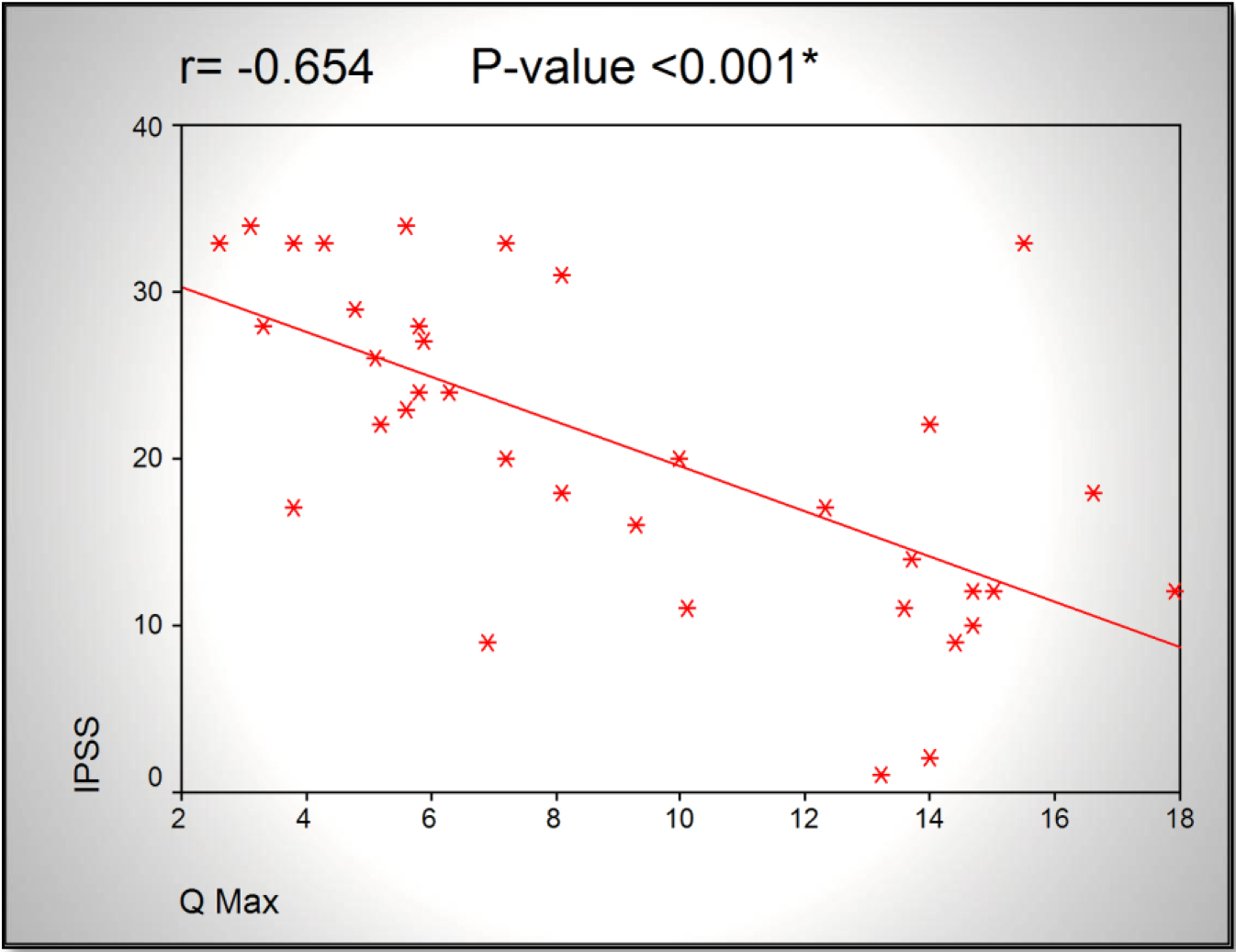
Figure 1.Scatter chart showing an inversely proportional relationship between Qmax and IPSS.

IJNUS 2019-102_Shady Emara_F2

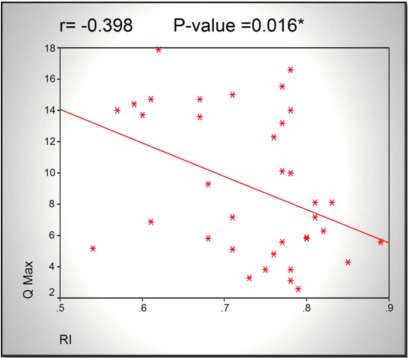
Figure 2. Scatter chart showing an inversely proportional relationship between RI and Qmax.

IJNUS 2019-102_Shady Emara_F3

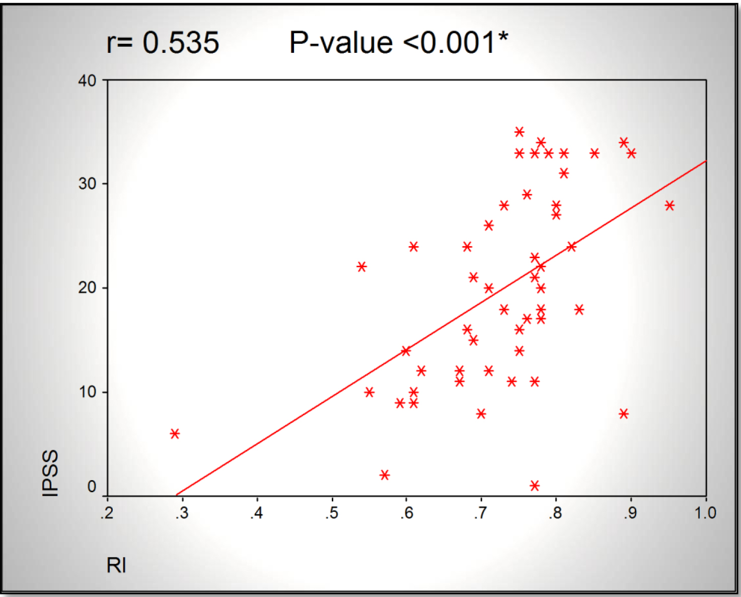
Figure 3. Scatter chart showing a directly proportional relationship between RI and IPSS.

#Sensitivity and specificity of RI:

Positivity of the test was assumed to be RI >0.71 (the upper limit of RI of normal prostatic capsular artery from Kojima study).

The diseased group was assumed to be those with Qmax< 10 ml/sec. (according to cut off established by Nitti et al 90% of men with a Qmax of less than 10 mL/sec are obstructed).

Discussion

Thanks to doppler imaging invention RI measurement in patients with LUTS has become a promising parameter for the diagnosis of BPH. It was found that a hyperplastic prostate tissue pushed the capsule out as it grew thus increasing the intraprostatic pressure as well as RI. The increase of the intraprostatic pressure is equally distributed throughout the whole prostate, so the increase of RI was found in both peripheral and transition zones [1]. In a Turkish study, the authors have intervened with Afluzosin XL 10 mg given to 34 patients with LUTSs for a month. They have found significant relationship between RI, Qmax, IPSS, and PSA. The mean RI value was 0.72+0.06 before medication and decreased significantly to 0.66+0.04 after the treatment (p<0.05). There was no relationship between RI and age (r=0.23, p>0.05). This study also depended on uroflowmetry rather than urodynamics [7].

In a study by Kojima M and colleges, they investigated the relationship between the resistive index (RI) of the prostate as measured by transrectal power Doppler with age, transrectal ultrasound planimetry and parameters of pressure-flow study.  A total of 140 elderly patients with lower urinary tract symptoms and no previous treatment for lower urinary tract symptoms, prostate cancer, bladder dysfunction or urethral stricture were investigated. A mean RI of 0.72±0.06 (range 0.59–0.88) was measured in patients with BPH versus a mean value of 0.64±0.04 (range 0.55–0.71) in those with a normal prostate (P<0.0001). The strongest correlation was found between RI and pdet (r = 0.401, P<0.005), followed by pdetQmax (r = 0.360,P<0.01) and the Abrams-Griffiths number (r = 0.330, P<0.05). This study depended on urodynamics to obtain the Pdet, thus bladder outlet obstruction index BOOI could be calculated and correlated with the RI. On the otherside, the authors didn’t mention IPSS as one of parameters for judging degree of bladder outlet obstruction [6]. The reason for the increase in RI in BPH has not been established, but it may be because the growing hypertrophic prostate pushes the capsule outward and thereby increases intraprostatic pressure and RIs [8].

In our study, 28 patients out of 52 (54%) were diagnosed obstructed i.e., Qmax less than 10 ml/sec, 21 (40%) patients were equivocal i.e., Qmax 10–15 ml/sec, and 3 patients (6%) were not obstructed i.e., Qmax more than 15 ml/sec. We have correlated between the resistive index, Qmax, IPSS, PSA, age, prostate volume, and adenoma volume. There was a significant increase in RI correlated to decrease in Qmax (r = –0.398, p < 0.016). Also there was significant increase in RI correlated to increase in IPSS (r = 0.535, p < 0.001). AS regard Qmax, there was significant decrease in Qmax correlated to increase in IPSS (r = –0.654, p < 0.001).

Conversely, no relation was found between degree of obstruction and other parameters; age, PSA, prostate volume, adenoma volume, residual volume.

At a cutoff of 0.71 the resistive index distinguished patients with and without bladder outlet obstruction with 71% sensitivity and 75% specificity, reflecting BOO severity in patients with BPH. At cut off of 0.8, RI is highly specific 100%, so it can strongly confirm the diagnosis of obstruction. Our results are consistent with those of Zhang X et al 2012, at nearly equal resistive index (0.71 in our study and 0.69 in Zhang study), the resistive index had sensitivity 71% compared to 78% in Zhang study. While specificity was 75% in our study, it was 86% in Zhang study.

The value of measuring the prostatic resistive index vs. pressure-flow studies in the diagnosis of bladder outlet obstruction caused by benign prostatic hyperplasia: TRUS is less invasive, cheaper and less time-consuming than pressure flow study, and measures prostatic size, which is useful in planning management [9]. Spectral waveform measurements by power Doppler transrectal ultrasonography may be useful in differentiating prostate cancer from benign hypertrophy [2]. One point of criticism was that we used uroflowmtery instead of urodynamics for assessing bladder outlet obstruction. However we obviated cases that may have detrouserhypocontractlity by excluding patients older than 70 years, excluding patients with suspected neurogenic element, and patients with very large residual volumes suggesting chronic retention.

Comparing results of our study with those of other studies:

Mean age:

Table 7. Comparing patient age in different studies

Study

Mean age (years)

Our study

63.9

Osama et al 2012

66.8

Hitoshi et al 2009

71.1

Zhang X et al 2012

67.5

Mean prostatic volume:

Table 8. Comparing prostate volume in different studies.

Study

Mean prostatic volume (grams)

Our study

82.9

Osama et al 2012

75.1

Hitoshi et al 2009

71.6

Zhang X et al 2012

53.5

Limitations of the study

When comparing values of RIs between IPSS groups (mild, moderate, severe), there was overlap between groups, i.e., some patients with mild symptoms had higher RI than some patients with moderate symptoms, and some patients with moderate symptoms had higher RI than some patients with severe symptoms, we attribute this overlap to the following:

Cases with only enlarged median lobe. It is hypothesized that an enlargement of the median lobe may not impact RI value as it does not impose increased resistance to capsular arteries. The association of intravesical prostatic protrusion (IPP) could add for a more precise diagnosis in this scenario [1]. There is some sort of selection bias. This group of age (55–70) mostly, will have cardiovascular risk factors placing further burdens on their prostatic blood flow. Prostate RI values are highly linked to overall metabolic syndrome and smoking in addition to BPH [10]. So, we recommend a study upon younger population in conjunction with cardiologists for assessing cardiovascular risk factors, thus excluding all factors than can influence RI other than pathology of BPH. IPSS questionnaire is sometimes a difficult task for the patient, and they tend to just complete it carelessly, this is due to many factors: poor vision in old age (which is the case of most patients with BPH), low level of education, or lack of interest.

Conclusion

RI can be used as a modality for assessing BPH patients and anticipating success of surgery. RI is a good indicator for degree of bladder outlet obstruction due to BPH, rather than other parameters as prostate volume, adenoma volume, residual volume, and PSA. Further research in this field will even allow the use of this modality to investigate other pathologies affecting the prostate and can be used also to evaluate the outcome of management.

Recommendation

We recommend a study upon younger population in conjunction with cardiologists for assessing cardiovascular risk factors like atherosclerosis, hyperlipdemia, and smoking. Thus excluding all factors than can influence RI other than pathology of BPH. Further studies in larger cohorts are required to validate the reliability of prostate capsular artery RI.

References

  1. Abdelwahab O, El-Barky E, Khalil MM, Kamar A (2012) Evaluation of the resistive index of prostatic blood flow in benign prostatic hyperplasia. International braz j urol 38: 255–257. [Crossref]
  2. Ahmet Tuncay Turgut, Esin Ölçücüoğlu, Pinar Koşar, Pinar Özdemir Geyik, Uğur Koşar, et al. (2007) et al. Power Doppler Ultrasonography of the Feeding Arteries of the Prostate Gland. Journal of Ultrasound in Medicine 26: 875–883.
  3. Yencilek E, Koyuncu H, Arslan D, Bastug Y (2014) The measurement of the prostatic Resistive Index is a reliable ultrasonographic tool to stratify symptoms of patients with benign prostatic hyperplasia. Medical Ultrasonography 16: 208–213. [Crossref]
  4. Ozden C, Gunay I, Deren T, Bulut S, Koparal S, et al. (2009) Effect of Doxazosin on prostatic resistive index in patients with benign prostate hyperplasia. Fırat Tıp Dergisi 14: 171–174.
  5. Tsuru N, Kurita Y, Masuda H, Suzuki K, Fujita K (2002) Role of Doppler ultrasound and resistive index in benign prostatic hypertrophy. International Journal of Urology 9: 427–430. [Crossref]
  6. Kojima M, Ochiai A, Naya Y, Okihara K, Ukimura O, et al. (2000) Doppler Resistive Index in Benign Prostatic Hyperplasia: Correlation with Ultrasonic Appearance of the Prostate and Infravesical Obstruction. European Urology 37: 436–442. [Crossref]
  7. Ayhan Karaköse, Turgut Alp, Numan Doğu Güner, Bekir Aras, Sabahattin Aydın (2010) The role of Doppler ultrasonography and resistive index in the diagnosis and treatment of benign prostate hyperplasia. TürkÜrolojiDergisi / Turkish Journal of Urology 36: 292–297.
  8. Kwon SY, Ryu JW1, Choi DH, Lee KS (2016) Clinical Significance of the Resistive Index of Prostatic Blood Flow According to Prostate Size in Benign Prostatic Hyperplasia. International Neurourology Journal 20: 75–80. [Crossref]
  9. Aldaqadossi HA, Elgamal SA, Saad M (2012) The value of measuring the prostatic resistive index vs. pressure-flow studies in the diagnosis of bladder outlet obstruction caused by benign prostatic hyperplasia. Arab Journal of Urology 10: 186–191. [Crossref]
  10. Baykam MM, Aktas BK, Bulut S, Ozden C, Deren T, et al. (2015) Association between prostatic resistive index and cardiovascular risk factors in patients with benign prostatic hyperplasia. The Kaohsiung Journal of Medical Sciences 31: 194–198. [Crossref]

The Introduction of Researches of Myofascial Release and Case Reports

Abstract

Myofascial release (MFR) is a technique for resolving fascial restriction; i.e., the fascia trapped with moderate pressure is continuously expanded to expand collagen fibers as well as fascial elastin fibers. In recent years fascia has increasingly been studied, as the roles and importance of fascia have become apparent. In many case reports pain and postural alignment have been designated as the outcome, and changes before and after MFR have been observed. Controlled studies have included a variety of researches for the presence or absence of the effects of MFR on patients with certain diseases, comparison of MFR with other techniques, and basic studies on the effects of MFR in healthy persons. It has been believed, however, that systematic reviews are of various quality levels because of the obscure content of intervention and insufficient exclusion of bias in spite of the favorable effects and the moderate quality of MFR techniques. The future task confronting us is thought to accumulate controlled studies, which will allow acquiring definite blinding and distinctly explaining fascial changes by detailed intervention methods.

Introduction

Myofascial release (MFR) is a technique for relieving fascial restriction; i.e., the fascia trapped with moderate pressure is expanded continuously, by which collagen fibers, as well as fascial elastin fibers, are expanded. Since MFR yields no any pain to the person treated by MFR without use of any specific tool, it can be used for every disease over all age groups; i.e., it is available for acute/chronic pain, restricted range of motion (ROM), conditioning in children and the aged, sports injury, and so on [1]. Some investigators have reported the origin of MFR. MFR is a fruit of soft tissue mobilization according to an American physical therapist, John F. Barnes [2], one of the Structural Integration (Rolfing®) techniques developed by an American biochemist, Ida P. Rolf [3], and a product of the technique developed by Thomas W. Myers [4], the author of “Anatomy Train”, who directly received training from Ida P. Rolf.

In recent years the roles and importance of fascia have become apparent, and at the same time fascia is being increasingly studied. Despite that MFR exerts the effects non-invasively on fascia via the superficial skin and fat layer, many MFR researches have designated changes in physical function, including changes in alignment and ROM, as the outcome. For this reason, the questions of whether fascia can be actually found or not and of how fascia changes remained. In recent years, however, imaging-out of fascia by an ultrasound imaging diagnostic device and observation of changes in the properties of fascia have become possible. This article introduces some previous researches for MFR with the author’s case reports. Self-MFR and foam roller MFR are excluded from the present study.

Previous Researches

Case reports

Barnes has reported treatment of a 35-year-old female patient who has suffered from thoracic outlet syndrome for 2 years. The 30-minute treatment including expansion of her upper limbs and MFR of the iliac muscle was conducted twice to three times a day for 2 weeks. Her pain was reduced, swing of her upper limbs during walking was normalized, kyphosis was improved, her body trunk and pelvis were restored to a median position, and the right-to-left load became even [5]. Le Bauer et al. have reported treatment of an 18-year-old female patient, who has suffered from bimodal scoliosis for 6 years. The 60-minute treatment including MFR involving her body trunk and expansion of her both lower limbs was conducted twice a day for 2 weeks. Postural alignment, X-ray images, pain, the condition with scale 22 based on the Scoliosis Research Society, and ROM of thoracolumbar rotation were markedly improved [6].

Martin has reported treatment of a female patient with diffuse systemic sclerosis. The treatment included 11 sessions of MFR involving the head and neck and 9 sessions of MFR involving her body trunk, and it took 60 minutes for each session. The treatment was conducted for 5 months, and symptoms of Raynaud’s phenomenon, thoracic mobility, and orificial distance were improved [7]. Walton has reported treatment of a 35-year-old female patient with primary Raynaud’s phenomenon. The 45-minute treatment including MFR of the region ranging from the neck to the dorsal surface of the chest and expansion of her upper limbs was conducted for 3 weeks. The duration and frequency of the appearance of Raynaud’s phenomenon and the severity of pain were decreased [8]. Many case reports have designated pain and postural alignment as the outcome and observed changes before and after MFR.

Controlled studies

Barnes et al. have divided 10 orthopedic outpatients into an MFR group of 6 patients who were treated with MFR [of the quadriceps muscle of thigh (QMT), iliopsoas muscle, and the contralateral iliopsoas muscle] for 10 minutes and a control group of 4 patients who were subjected only to lie on a bed for 10 minutes, and compared both groups concerning lateral tilt angle of the pelvis [the mean difference in the distance between the right and left anterior superior iliac spine (ASIS) and the central point at patient’s feet]. The difference in the distance was significantly reduced in MFR group, increasingly showing the symmetric form of the pelvis [9]. Takeda et al. have conducted MFR of the greater pectoral muscle and smaller pectoral muscle in 25 patients with retentive hemiplegia, and compared the angle of abduction of the shoulder on the affected side, speed and the degree of easiness of patients’ daily living lives, and 10-meter walking speed before and after MFR. They have reported the significant improvement in the abduction angle and the speed of the patients’ daily living lives [10]. Marszaiek has conducted MFR of the head, neck, upper limbs, and the upper body trunk in 40 patients who have undergone total laryngectomy. The esophageal pressure was significantly decreased after MFR, having led to easy training of esophageal phonation [11]. Some other reports have shown that MFR of the head and neck in patients with the forward head posture has induced the significant improvement in the craniospinal angle, neck disability index, and cervical ROM [12, 13] and that MFR of the body trunk involving the low back in low back pain patients has induced significant improvement in pain and the influence of low back pain on daily living activities [14–16].

Kain et al. have compared each ROM of flexion, extension, and abduction of the shoulder between an MFR group of 18 healthy subjects who underwent precordial MFR for 3 minutes and a hot pack group of 13 healthy subjects who underwent hot pack for 20 minutes. Both groups showed significantly increased ROM, compared to that before the implementation, except that only the flexion angle was significantly higher in the MFR group than in the hot pack group [17]. Henley et al. have compared heart rate on a tilt (50°) table, normalized ECG, and respiration rate between an MFR group of 17 healthy subjects who underwent MFR of the neck for 2 minutes and a pseudo-MFR group of 17 healthy subjects with their neck only touched by rater’s hands. Tachycardiac rate and normalized ECG were significantly increased in both groups, compared to those at rest, whereas the tachycardiac rate and the normalized ECG were lower in the MFR group than in the pseudo-MFR group [18].

Kuruma et al. have compared ROM of knee joint flexion, muscle stiffness, and reaction time among a QMT-MFR group of 10 healthy subjects who underwent MFR of the QMT for 8 minutes, a hamstrings (H)-MFR group of 10 healthy subjects who underwent MFR of H for 8 minutes, and a stretching group of 10 healthy subjects who underwent stretching of QMT. All groups significantly showed improvement in ROM, while reaction time was significantly reduced in the QMT-MFR and H-MFR groups [19]. Ichikawa et al. have compared muscle stiffness and the fascial transmission distance on ultrasonic images among an MFR group of 12 healthy subjects who underwent MFR of the lateral great muscle for 4 minutes, 10-min-hot-pack group of 12 healthy subjects who underwent hot pack for 10 minutes, and 20-min-hot-pack group of12 healthy subjects who underwent hot pack for 20 minutes. There were significant changes in muscle stiffness and the fascial transmission distance only in the MFR group [20].

We have compared angles of active and passive extension and elevation of lower limbs and muscle strength (extension/flexion of the knee joint) before intervention and for 6 days after intervention among an H-MFR group of 10 healthy subjects who underwent MFR of hamstrings (H), a QMT (re-education)-MFR group of 10 healthy subjects who underwent muscle re-education exercises of QMT (40 times at muscle strength of 40% of 1 repetition maximum) following MFR of H, and an H (re-education)-MFR group of 10 healthy subjects who underwent muscle re-education exercises of H following MFR of H. Improvements in the extension and elevation angles for the lower limbs and the muscle strength of knee flexion were much more in the H (re-education)-MFR group than in two other groups. There were also significant differences between those 6 days after and before the implementation. In the H-MFR group there were significant differences in the angle of extension and elevation of lower limbs and muscle strength of knee flexion between those for 4 days after and before MFR [21]. To investigate the fascial properties after MFR, we clarified intra-rater reliabilities [ICC (1, 1)] 4 days after measurements of superficial and deep fascial transmission distances on ultrasound images of lateral head of the gastrocnemius muscle by using an ultrasound imaging diagnostic device and measurement of muscle stiffness according to real-time tissue elastographic function (superficial layer: 0.89; deep layer: 0.98; muscle stiffness: 0.90) [22]. We compared ROM of ankle dorsal flexion, muscle strength of ankle plantar flexion, fascial transmission distance, and muscle stiffness before and after intervention and for 4 days after intervention between an MFR group of 17 healthy subjects who underwent MFR of the lateral head of gastrocnemius muscle for 3 minutes and a stretching group of 17 healthy subjects who underwent static stretching for 3 minutes. In both groups, ROM and fascial transmission distance were increased and muscle stiffness was decreased immediately after the intervention, compared to those before intervention. Immediately after the intervention muscle strength was increased in the MFR group and decreased in the stretching group, while ROM, muscle strength, and fascial transmission distance were increased and muscle stiffness was decreased 4 days after the intervention than those before the intervention only in the MFR group [23]. Thus, there have been a variety of controlled studies including comparative studies on the presence/absence of the effects of MFR on patients with certain diseases and between MFR and other techniques, as well as basic researches of the effects of MFR on healthy persons.

Systematic reviews

Yang et al. [24] have inspected 1329 references in the literature concerning chest physiotherapy for pneumonia in adults in 2010, which included 6 references of randomized controlled trials (434 subjects). As a result, it was revealed that osteopathic therapy including MFR allowed admission period and the duration required for intravascular and systemic antibiotic treatment having been decreased, although any symptom of pneumonia or X-ray finding was not improved [22]. Yuan et al. have investigated minutely 532 references in the literature concerning treatment for fibromyalgia in 2015, and 2 references about randomized trials of MFR (145 subjects) were included in meta-analysis. As a result, it was revealed that MFR had moderate evidence of its effects particularly on pain, anxiety, and depression [25]. McKenney et al. have examined closely 88 references in the literature to investigate the quality and reliability of MFR in 2013, and 10 references of randomized trials were included. Ajimsha et al. have also investigated 3 systematic reviews in 2019. The thus-described researchers’ studies have provided evidence of the favorable effects of MFR and the moderately technical quality, but according to them, it has various degrees of quality for the reason that the intervention contents are obscure and that bias is insufficiently removed. They have brought their researches to a conclusion by saying that individual systematic review will become a beginning toward future investigation of higher quality [26, 27].

Case reports

The author encountered 2 patients who acquired characteristic improvement as a result of MFR. These cases are introduced below. The first case was a male patient in his 50s, a physician, whose chief complaint was low back pain. When he tried to stand up after morning medical examination, he could not stand up because of low back pain. As for sites of low back pain, he had both lumbar regions, but the pain was particularly severe in the right region. He had no idea of any event by which low back pain was manifested in his recent daily activities. According to inquiries about his past history, he had right second metatarsal capital fracture 6 months ago. He has been unable to bear any load on the affected site and shown claudication because of pain for a while. At present, he had no pain in the right second metatarsal bone. He felt low back pain in getting-up and standing positions and during walking. Since he had pain when load was given to the affected site, evaluation was started with his feet on the assumption that the right second metatarsal capital fracture was responsible for low back pain. Subsequently, high-density regions were recognized in the right long extensor muscle of great toe, right anterior tibial muscle, lateral head of the right gastrocnemius muscle, right biceps muscle of thigh, right iliac muscle, bilateral lumbar iliocostal muscle, and bilateral lumbar quadrate muscles. Except for the lumbar quadrate muscles, it was considered that claudication to avoid using the second metatarsal bone resulted in the condition in which fascial dysfunction has spread along the anterior and posterior motion arrangement (referred to the concept of fascia and fascial approach) (Figure 1). Faced with this situation, we considered the feet as the cause of the condition, and we conducted MFR on each of the right long extensor muscle of great toe, right anterior tibial muscle, and lateral head of the right gastrocnemius muscle for 3 minutes. After MFR, low back pain was reduced from score 8 to score 3 based on the Numerical Rating Scale. When MFR was conducted on each of the bilateral lumbar iliocostal muscles for 2 minutes, low back pain disappeared and he felt no physical disorder at his low back. His subsequent course also appeared favorable.

IJOT 19 SI - 104_Yasuki Katsumata_F1

Figure 1. Fascia showing the ascending spread of high-density areas.

The second case was a male patient in his 80s, and diagnosed as having had left middle cerebral arteriosclerosis. Owing to (rt-PA) thrombolysis, paralysis was improved from complete paralysis to moderate right hemiplegia. It was improved even to mild paralysis by 3-week rehabilitation, and he acquired retentive self-supporting in a standing position and walking without support with light assistance. However, improvement of function of swallowing was worse than that of physical function. It was assumed from postural evaluation that anterior cephalic presentation and unbalance between the right and left postural alignments (effortive on the non-affected side) inhibited movements of the masticatory muscle and muscles of tongue. On this assumption, MFR of the suboccipital muscles, left sternocleidomastoid muscle, suprahyoid muscles, posterior region of neck, and upper fibers of left trapezius muscle, and expansion of the left upper limb were conducted for 40 minutes a day for 3 days. As a result, the anterior cephalic presentation was improved (Figure 2), the right and left postural alignments showed symmetric balance (Figure 3), and the swallowing function was also improved (Table 1).

IJOT 19 SI - 104_Yasuki Katsumata_F2

Figure 2. Postural alignment on the sagittal plane (rightward motion) before and after the treatment.

IJOT 19 SI - 104_Yasuki Katsumata_F3

Figure 3. Postural alignment on the frontal plane (ante-motion) before and after the treatment.

Table 1. Evaluation of the swallowing function before and after the treatment.

Before intervention

After intervention

Swallowing

Swallowed after several times

Swallowed after once or twice

The amount ingested

1/3 spoonful

a spoonful

Pharyngeal residue

(+)

(±)

Cough

(+) immediately after meals

(+) after some mouthfuls

Tongue protrusion

(-)

(+)

Conclusion

Establishment of evidence of the effects of MFR seems to be delayed, while approach to fascia is increasingly spreading along with the increasing recognized importance of fascia. The future task confronting us is thought to accumulate controlled studies, which will allow distinctly explaining fascial changes under the condition of definite blinding by detailed intervention methods.

References

  1. Takei H (2001) Myofascial Release. Rigakuryoho Kagaku. Apr: 103–107 (Japanese).
  2. Barnes JF (1990) How It Bagan Myofascial Release the search for excellence. Washington, USA: National Library of Medicine Pg No: 1–2.
  3. Yasushi F (2005) An Outline of Rolfing. Japanese Journal of Complementary and Alternative Medicine. Feb: 37–43(Japanese).
  4. Earls J, Myers TW (2010) An Introduction to Fascial Release Technique Fascial Release for Structural Balance Chichester, UKB: Lotus Publishing Pg No: 4–16.
  5. Barnes JF (1996) Myofascial release in treatment of thoracic outlet syndrome. J Bodyw Mov Ther  Jan: 53–57.
  6. LeBauer A, Brtalik R, Stowe K (2008) The effect of myofascial release (MFR) on an adult with idiopathic scoliosis. J Bodyw Mov Ther 12: 356–363. [crossref]
  7. Martin MM (2008) Effects of the myofascial release in diffuse systemic sclerosis. J Bodyw Mov Ther Apr: 1–9.
  8. Walton A (2008) Efficacy of myofascial release techniques in the treatment of primary Raynaud’s phenomenon. J Bodyw Mov Ther Pg No: 274–280.
  9. Barnes MF, Gronlund RT, Little MF, Personius WJ (1997) J Bodyw Mov Ther. Oct: 289–296.
  10. Takeda S, Takahashi K, Kawasaki T, Kaneko T, et al. (2005) Ijikinouso cchuukatamahi kanja Mahisoku kyoubukingunn henokinnmakuriri- sunoouyou [abstract] Rigakuryouhougaku  32(Suppl 2): ID-868 (Japanese).
  11. Marszaiek S (2009) Estimation of influence of myofascial release techniques on esophageal pressure in patients after total laryngectomy. Eur Arch Otorhinolaryngol May: 1305–1308.
  12. Kim J, Kim S, Shim J, Kim H (2018) Effects of McKenzie exercise, Kinesio taping, and myofascial release on the forward head posture. J Phys Ther Sci Pg No: 1103–1107.
  13. Aggarwal A, Shete AV, Palekar TJ (2018) Efficacy of Suboccipital and Sternocleidomastoid Release Technique in Forward Head Posture Patients With Neck Pain: A Randomized Control Trial. Int J Physiother Pg No: 149–155.
  14. Tozzi P1, Bongiorno D, Vitturini C (2011) Fascial release effects on patients with non-specific cervical or lumbar pain. J Bodyw Mov Ther 15: 405–416. [crossref]
  15. Ajimsha MS, Daniel B, Chithra S (2014) Effectiveness of myofascial release in the management of chronic low back pain in nursing professionals. J Bodyw Mov Ther 273–281.
  16. Arguisuelas MD, Lison JF, Domenech-Fernandez J, Martinez-Hurtado I (2019) Effects of myofascial release in erector spinae myoelectric activity and lumbar spine kinematics in non-specific chronic low back pain: Randomized controlled trial. Clin Biomech (Bristol, Avon) 27–33.
  17. Kain J, Martorello L, Swanson E, Sego S (2010) Comparison of an indirect tri-planar myofascial release (MFR) technique and a hot pack for increasing range of motion. J Bodyw Mov Ther 63–67.
  18. Henley CE, Ivins D, Mills M, Wen FK, et al. (2008) Osteopathic manipulative treatment and its relationship to autonomic nervous system activity as demonstrated by heart rate variability a repeated measures study. Osteopath Med Prim Care 2–7.
  19. Kuruma H, Takei H, Nitta O, Furukawa Y, et al. (2006) Kinmakuriri-su to sutorecchingu womochiita rigakuryouho ukouka no hikakukentou [abstract] Rigakuryouhougaku 2006; 34 (Suppl 2) ID-259 (Japanese).
  20.  Ichikawa K, Takei H, Usa H, Mitomo S, et al. (2015) Comparative analysis of ultrasound changes in the vastus lateralis muscle following myofascial release and thermotherapy: a pilot study. J Bodyw Mov Ther 327–336.
  21. Katsumata Y, Takei H, Hori T, Hayashi H (2016) Influences of muscle re-education exercises for myofascial extensibility and muscle strength after myofascial release. Rigakuryoho Kagaku 99–106.
  22. Katsumata Y, Takei H, Hayashi H, Ichikawa K (2017) Intra- and Inter-rater Reliabilities of measurements of fascial displacement and muscle stiffness by using ultrasound images. Rigakuryoho Kagaku 215–220 (Japanese).
  23. Katsumata Y, Takei H, Sasaki Y, Watanabe K (2019) Ultrasonographic changes in fascial properties over time after myofascial release. Integr J Orthop Traumato 1–6.
  24. Yang M, Yuping Y, Yin X, Wang BY, et al. (2010) Chest physiotherapy for pneumonia in adults. Cochrane Database Syst Rev CD006338.
  25. Yuan SL, Matsutani LA, Marques AP (2015) Effectiveness of different styles of massage therapy in fibromyalgia: a systematic review and meta-analysis. Man Ther 257–264.
  26. McKenney K, Elder AS, Elder C, Hutchins A (2013) Myofascial release as a treatment for orthopaedic conditions: a systematic review. J Athl Train 522–527.
  27. Ajimsha MS, Shenoy PD (2019) Improving the quality of myofascial release research – A critical appraisal of systematic reviews. J Bodyw Mov Ther 561–567.

Fascial Manipulation® for Trigger Finger (Snapping Finger)

Summary

A 41-year-old female patient, who developed trigger finger after she repeated cervical sprain several times, underwent myofascial evaluation and treatment, which were based on Fascial Manipulation®, in addition to evaluation by physical therapy, and favorable results were obtained. She showed symptoms of trigger finger, which suddenly occurred, for 5 months. Palliative treatment was the only method for the symptoms, and they did not reach improvement. The site and tissue, which are responsible for the condition, were specified first on evaluation by physical therapy. Subsequently addition of exercise test and palpation test for fascia in view of a past history and timeline may appropriately approach to problems with high-density sites and force transmission of the fascia related to pain.

Introduction

Many cases of trigger finger have been believed to be idiopathic, and the symptoms occur spontaneously. Some reports have indicated the relevance to occupational or repetitive activities [1]. For the pathogeneses, much attention was paid to specification of sites of myofascial dysfunction in view of a past history and living activity level and routes of force transmission, as well as conventional tests and evaluation. This article describes favorable results of the myofascial evaluation and treatment, which were based on Fascial Manipulation® (FM®) and conducted in addition to evaluation by physical therapy, in a patient who developed trigger finger after she repeated cervical sprain several times.

Roles of fasciae

Fascia has been explained at the International Conference of Scientific Research of Fascia, as follows: “Fascia, a soft tissue constituent of the connective tissue system all over the human body, forms a 3-D matrix in the whole body to support structures “[2]. Fascia spread over all organs, muscles, bones, and nerve fibers to cover them. The definition of fascia includes aponeurosis, ligament, tendon, retinaculum, articular capsule, capsules of organs and vessels, epineurium, meninges, periosteum, and intra- and intermuscular fibers of all fasciae. All of them indicate that fasciae have important roles in muscular biomechanics, coordination of muscular peripheral movements, and maintenance of proprioceptor and postures.

Some muscle fibers of epimysium enter the deep fascia; i.e., 37% of muscle origins and insertions enter the deep fascia and intermuscular septum (myofascial expansion) without insertion and the inserted tendon [3]. When fascial dysfunction occurs, muscle spindle and nociceptor are stimulated, spreading along the fascial arrangement via the deep fascia. For instance, aponeurotic fasciae cover the whole muscles of the upper limb, and collagen fiber bundles are arranged in different directions in the aponeurotic fasciae. The thoracic muscles receive tension at a proximal site by insertion of various fasciae, enabling to slide between them and inferior muscles. The brachial fasciae are connected at a proximal site to axillary fascia, greater pectoral fascia, deltoid fascia, and dorsolateral fascia, while they are connected to antebrachial fascia at a distal site. The mediolateral intermuscular septum is originated from the brachial fascia, by which the upper arm is divided into the front and the rear parts as segments. At the elbow the brachial fascia is reinforced by the anterior and rear retinacula, and the anterior retinaculum is composed of the brachial biceps aponeurosis. The brachial biceps aponeurotic expansion branches off two directions. In one direction a fiber bundle extends like a bow obliquely and medially below and binds at the antebrachial fascia. Inside the elbow many muscle fibers of the round pronator muscle and radial carpal flexor are inserted into the antebrachial fascia from the inside. In the other direction collagen fiber bundles are running in parallel to a median line of the forearm in a longitudinal direction. This fibrous expansion reaches the antebrachial fascia between the radial carpal flexor and the humeroradial muscle. Therefore, when the brachial biceps (muscle) tendon is extended at a proximal site, two force lines appear in a medial direction corresponding to the coved fibers and in a direction longitudinally running along the central part of the forearm.

On movements of the upper limbs in various directions, fascial expansion activates fascial proprioceptor with a specific moving pattern and extends a specific site of the brachial fascia, connecting different sites to transmit force. Owing to the relationship between the muscle and fascia coordinative movement to the periphery is realized by performance of movement in a correct direction and correct recognition [2, 4].

Fascia has a role in enhancement of muscle sliding. There is hyaluronic acid in loose connective tissue between deep fascial layers and between epimysium and endomysium, which acts as a lubricant [5]. When hyaluronic acid aggregation is induced by trauma, overuse, etc., fascial layer sliding is restricted. Contraction of the epimysium causes tendon extension due to high density of epimysium, and the extension stimulates the articular receptor to lead to its excitement and pain around the joint. When the body has pain, it responds to the pain with secondary compensation by a posture to avoid the pain. The change in base tension due to the compensation will be controlled by up-and-down tension on the competitive or ipsilateral side, leading to increased complication of the symptoms [6].

FM®

The subjects of FM® treatment include the point [referred to by Centre of Coordination (CC)] on the epimysium, to which one-way muscle strength converges, and the point [referred to by Centre of Fusion (CF)], to which force of adjacent two deep fascia (aponeurotic fascia) units converges. The body is divided into 14 segments, and a functional unit related to movement in each direction is called as fascial unit. All the segments include 6 CC points. There are 6 directions of movement: Sagittal plane (antemotion: AN and retromotion: RE); frontal plane (lateromotion: LA and mediomotion: ME); and horizontal plane (extrarotation: ER and intrarotation: IR). Each fascial unit is designated from the movement direction and segment. For example, the fascial unit of anterior movement of CU (elbow) is designated as AN-CU. There are 4 directions of movement of CF: Anterio-lateral (Ante-Latero: AN-LA); anterior-medial (Ante-Medio: AN-ME); retrolateral (Retro-Latero: RE-LA); and retromedial (Retro-Medio: RE-ME) [6,7]. CC forms the one-way continuous arrangement (called as fascial arrangement) associated with movement direction along the sagittal, frontal, and horizontal planes [8]. For example, the facial arrangement of anterior movement of the upper limbs is composed of 5 fascial units, i.e., AN-SC (scapula), AN-HU (upper arm), AN-CU, AN-CA (carpus), and AN-DI (finger), and anterior movement of the upper limbs is induced by the arrangement. CF has a fascial diagonal line, which appears on a diagonal line of fascial arrangement, and a fascial spiral, which integrates articular elements with retinaculum to influence wide-range pain. It comes to be important for treatment which arrangement has a problem [6, 7].

Pathogeneses of Trigger Finger (Snapping Finger)

Trigger finger is tenosynovitis of the flexor tendon due to imbalance between the tendon sheath and the flexor tendon passing the sheath. Transmission disorder occurs in the tendon sheath to lead to pain, swelling, and heat sensation of fingers. It has been reported that thickening of the tendon sheath, ligamentous intrathecal narrowing, edematous enlargement of the tendon itself, and so on are responsible for these conditions [9]. The augmentation of the symptoms early in the morning and amelioration of the symptoms by day are frequently observed. When they advance, a snapping phenomenon develops, and it may ultimately result in secondary contracture of the Proximal Inter Phalangeal (PIP) joint. The symptoms also frequently appear in a plurality of fingers. It has been believed that the phenomenon is one of the most common causes of hand pain in adults. It has also been reported that the prevalence is ca. 2% of the general population, and tends to be high in women in their fifties or sixties. The prevalence in women in the later stages of pregnancy is also high, and the condition is also characterized by its frequent occurrence due to overuse of hand and as sports injury. It frequently occurs in patients with diabetes, rheumatoid arthritis, or those under the conditions such as amyloidosis, in which systemic accumulation of proteins occurs. As for the treatment, some investigators have reported evidence of moderate efficacy of conservative intervention including the short-term use of Non-Steroidal Anti-Inflammatory drug (NSAID) [10]. The orthotic treatment has also been widespread [11]. In case of conservative therapy, surgical treatment may also be selected when any improvement is not achieved by conservative therapy.

Treatment case

1. General information

A patient is a 41-year-old woman, housewife.

The chief complaints included flexion contracture of and resting pain in the left thumb MP joint and thumb movement pain, and she grasped with difficulty because of pain.

Approximately 5 months ago she suddenly had left thumb pain and restricted Range of Motion (ROM) at the time of rising from her bed. In the early stage the pain was gradually reduced by day, but in the next morning she repeated pain and restricted ROM. The pain gradually augmented even by day. She visited a hospital, and received intrathecal steroid injection with a diagnosis of trigger finger. Even so, the symptoms were not improved. Subsequently she had an attempt to receive acupuncture as well, but the pain augmented. Her left thenar swelling also appeared, and she could do daily living activities (ADL), including clothespin pinching, taking out coins, grasping dish and mobile phone, etc., with difficulty. Thus, she came to interfere with the whole range of housework.

Diagnosis: Trigger finger (snapping finger)

Past history:

20 years of age: Cervical sprain-due to numbness in the region ranging from neck to left hand (traffic accident)

25 years of age: Surgery for right inguinal hernia

30 years of age: Cervical sprain-due to numbness in the region ranging from neck to left hand (traffic accident). Treated by cervical collar fixation

36 years of age: Cervical sprain-due to numbness in the region ranging from neck to both hands (traffic accident)

38 years of age: Right 5th metatarsal fracture

39 years of age: Cervical sprain (a violent fall)

In her late thirties she repeated pain around the scapula once or twice a year.

41 years of age: Lt Thumb trigger finger (snapping finger)

2. Evaluation by physical therapy

Pain: Resting pain (+), movement pain (+), numbness (-)

Active movement: ROM restriction in all directions of left thumb CM joint, in association with pain with score 8 based on the Numerical Rating Scale (NRS).

Passive movement: ROM restriction in all directions of left thumb CM joint, in association with NRS 8 pain.

Neurological test: Various neurological tests (-)

End feel: Empty

Joint play test: Hypermobility of C4th/5th and 5th/6th; low mobility of TH1st/2nd.

Muscle tightness: Brachioradial muscle, long palmar muscle, round pronator muscle, biceps muscle of arm, scalenus, and smaller pectoral muscle.

Observation of posture: Round back and forward head.

Observation of motion: Difficult movements of grasping and pinching.

3. Hypothesis

This patient developed numbness in her both upper limbs after she sustained cervical sprain several times. Since she had a past history of cervical collar fixation, her cervical vertebrae were examined. Various neurological tests are negative at present. She repeated cervical sprain, and had the imbalanced trunk because of coexistence of hypermobility of the cervical vertebrae with low mobility of the thoracic vertebrae. The patient may have been forced to have compensation for various postures under the situation with her unstable neck. It was further considered that the poor alignment accelerated excessive tension of her neck and chest to have led to tension stress to her left thumb through fascial arrangement and expansion from the trunk to the upper limbs. On the hypothesis that the stress spread from the cervicothoracic vertebrae downward, fascia was evaluated.

4. Palpation test [High density level (*~***)]: Comparative palpation test was conducted in TH (thorax), SC, and CA. LT LA-CA***, Bi LA-TH***, Lt LA-SC**, Rt LA-CL (neck)**, Lt ME-CA**, and Lt ME-CU**.

Palpation test revealed high density at the above-described sites, indicating remarkable areas of high density on the frontal plane arrangement.

5. Treatment

First treatment: Lt LA-CA (Figure 1), Lt LA-CU, Lt LA-DI (Figure 2), Lt ME-DI (Figure 3), and Lt ME-CA (Figure 4) (++).

IJOT 19 SI - 103_Atushi Yoshida_F1

Figure 1. Lt LA-CA.

IJOT 19 SI - 103_Atushi Yoshida_F2

Figure 2. Lt LA-DI.

IJOT 19 SI - 103_Atushi Yoshida_F3

Figure 3. Lt ME-DI.

IJOT 19 SI - 103_Atushi Yoshida_F4

Figure 4. Lt ME-CA.

Second treatment: Lt LA-CA, Lt LA-SC (Figure 5), Rt LA-CL, Lt ME-CU, and Bi LA-TH (Figure 6) (+++).

IJOT 19 SI - 103_Atushi Yoshida_F5

Figure 5. Lt LA-SC.  

IJOT 19 SI - 103_Atushi Yoshida_F6

Figure 6. Lt LA-TH.

6. Treatment results

Although pain on grasping movement was reduced and ROM was improved after the first treatment, she complained of tension on her neck and upper back. One week later she received the second treatment, and pain on pinching movement, restricted ROM, and a sensation of tension on her upper back disappeared.

Discussion

The patient repeated cervical sprain, and had numbness in the region ranging from her neck to fingers. However, the region was not consistent with the dermatome of the C4th/5thor 5th/6th, which showed cervical hypermobility, and the site of numbness varied day by day. The patient’s condition repeated remission and exacerbation. Her life in such a situation is presumed to have caused various compensatory postures and activities. One of these causes is fascial compensation. Excessive tension of her trunk, which is originated from cervical instability, is considered to have received stress through fascial expansion to the hand along the arrangement of fascial connection. For this reason arrangement of fascial balance between the proximal and distal positions may have led to reduction in symptoms by intervention along the arrangement.

Conclusion

This article described the importance of evaluation and treatment with FM® from a musculofascial viewpoint for a patient who developed trigger finger after she repeated cervical sprain several times.

It has been believed that the occurrence of trigger finger is idiopathic. The symptoms appear spontaneously and have correlation with occupational or repetitive activities. The condition shows compensatory movements due to fascial dysfunction very frequently. Not only palliative treatment of the present symptoms but also specification of the causative sites and tissue by physical therapeutic evaluation may make an appropriate approach possible to resolve problems with the high-density site of pain and force transmission by addition of movement test and precise palpation test for fascia in view of a past history and the timeline. It is further important for trigger finger patient to do exercise for correction of compensatory movements after improvement in fascial sliding and the high-density site and to advance the movement to functional movement and to ADL movement.

References

  1. ……………………………
  2. Atsushi Yoshida (2019) The interaction between muscle and fascia (myofascial chain).  Spine & Spinal Cord. 32: 301–306.
  3. …………….
  4. Stecco C (2018) Atlas of Functional Anatomy of Fascial System.  Hitoshi Takei (Tr.). Ishiyaku Publishers, Inc. : 234–291.
  5. Hitoshi Takei (2014) Expansion of Systemic and Therapeutic Technique.  H. Takei, et al. (Ed.). KYODO ISHO SHUPPAN CO., LTD., Tokyo.
  6. Atsushi Yoshida (2015) Practical approach to muscle and fascia (Special Issue: Manipulative physical therapy for sports injury). The Journal of Clinical Sports Medicine. 32: 1000–1004.
  7. Stecco L et al (2011) Fascial Manipulation—Theory Edition. H. Takei (Tr.) Ishiyaku Publishers, Inc., Tokyo.
  8. Schleip et al (2015) Membrane and Fascia. Up-to-date knowledges and therapeutical approach. H. Takei (Tr.), Ishiyaku Publishers, Inc., Tokyo, 343–349.
  9. Misako Nishimori: Pathological characteristics of tenosynovitis of the flexor tendon (trigger finger) on ultrasonic images of the joint.  Japanese Journal of Medical Ultrasound Technology. 38: 2013.
  10. ……………….
  11. ………………..

Treatment for low back pain using Fascial Manipulation

Introduction

Fascial Manipulation® (FM®), a modality of manipulative physical therapy originated with an Italian physical therapist, Luigi Stecco, is classified roughly into two types, i.e., FM® for musculoskeletal dysfunction and FM® for internal dysfunction.  In the FM® for musculoskeletal dysfunction, a route to fascial compensation is revealed from results of inquiries, exercise test, and palpation test, and then points of Center of Coordination (CC) and Center of Fusion (CF), which are associated with the compensation, are treated.  In general, FM® is therapeutically designed to recover the feature of sliding of the deep fascia and to improve patient’s pain, Range of Motion (ROM), and muscle strength [1,2]. Focusing on low back pain, which physical therapists and physicians frequently encounter and treat in clinical settings, practical cases of FM® for musculoskeletal dysfunction are mentioned through 2 case reports in this article.

Practical cases of FM®

Case 1 – Ascending Fascial Compensation

General information

A 32-year-old woman, a care worker, has started playing badminton since her age of 10 years.  At present she plays badminton about once a month.  The physician who examined the patient made a diagnosis of myofascial low back pain, as any distinct finding on X-ray or MRI image was observed, and treated the patient by physical therapy.

Inquiries

The chief complaint of the patient was left low back pain (at the level of the 4th-5th lumbar vertebrae).  She had the pain 6 months ago without manifestation by any overt symptom.  It was caused by the long-time standing position and assistance for transfer activities during the work.  She had no pain in her sitting or lying position.  The most severe pain showed score 7 based on the Numerical Rating Scale (NRS). The patient has always been feeling physical disorder at her medial left scapula since 3 months ago (NRS: 1-2).

Inquiries about past histories revealed that the patient had fracture of the distal end of the right radius one year ago and received the 4-week treatment by plaster fixation.  She had pain in the lateral region of the left elbow joint 10 years ago.  The longest past history was left ankle joint inversion sprain 17 years ago.  It was treated by plaster fixation for 3 weeks, and it needed 4 months to have fully recovered. The patient had no dysesthesia at any terminal point (head, fingers, or toes), surgical history, or non-contributory internal past history.

Hypothesis

In FM® a hypothesis is built up regarding a route to fascial compensation from temporal/spatial viewpoints on the basis of the results of inquiries [1]. Figure 1 shows a timeline of information, which was collected on inquiries about the chief complaint (the most severe pain at present), its associated pain, and past histories of he patient.  Figure 2 shows a body chart including the same information as that in Figure 1.

IJOT 19 SI - 102_Daisuke Ogawa_F1

Figure 1. A timeline (case 1).

IJOT 19 SI - 102_Daisuke Ogawa_F2

Figure 2. A body chart (case 1).

Several hypotheses can be built up about the route to fascial compensation from Figures 1 and 2.  When the occurrence of low back pain as chief complaint in a standing position is taken into consideration, however, insufficient sliding of the deep fascia may have been induced by long-term plaster fixation of the left ankle during the treatment of ankle inversion sprain [1], probably leading to the ascending fascial compensation and left low back pain in the patient.

Evaluation by the therapist

(1) Exercise test

On the basis of the above-mentioned hypothesis, two segments, i.e., pelvic girdle (PV) and ankle joint (TA), were selected for exercise test.  As a result, the same type of pain (NRS: 6) as the chief complaint, was induced to PV by pelvic anterior tilt movement in a standing position, while no marked finding was observed in TA.

(2) Palpation test

The segments selected first for palpation test were PV, i.e., segment of the chief complaint, TA, i.e., the origin of the fascial compensation, and the hip joint (CX) localized between the PV and TA segments.  As for these segments, all CC points (anterior, rearward, inward, outward, internal rotation, and external rotation) were palpated. As a result of palpation test for CC, there was no difference in the number of the points at which findings of high density were observed, or the degree of high density among sagittal planes (anterior/rearward), frontal planes (inward/outward), and horizontal planes (internal rotation/external rotation), suggesting that fascial diagonal or fascial spiral, rather than fascial arrangement, is involved with fascial compensation.  Therefore, palpation test for CF points of the above-mentioned three segments was conducted, revealing that CF of left RE-LA-PV1 (Figure 3) showed a large area of high density and had remarkable pain associated with irradiating pain.  As other findings, left RE-LA-TA2 and left Re-LA-CX showed moderately high density.

IJOT 19 SI - 102_Daisuke Ogawa_F3

Figure 3. Palpation and treatment for RE-LA-PV1 CF.

It was considered from the results of palpation test for the PV, TA, and CX that a left RE-LA diagonal or a left AN-ME spiral was involved with the patient’s chief complaint.  Faced with this situation, CF points were palpated at RE-LA and AN-ME of segments of toes (PE) and knee joint (GE) on the left side and low back (LU), and thorax (TH) on both sides.  As a result, left RE-LA-TH showed findings of a large area of high density, and left RE-LA-PE3 and RE-LA-LU on both sides showed findings of moderately high density.  It was judged from these findings that a left RE-LA diagonal was mostly involved with the patient’s chief complaint.  Then, the patient was treated based on the evaluation.

Treatment

In FM® the CC/CF points treated are selected, and routes to fascial compensation are taken into consideration even on determining the treatment order [1, 2].  In general, since CC/CF points of segments with the chief complaint frequently show serious pain, the treatment rarely starts with the segments. In this patient the treatment started with RE-LA-PE3 (Figure 4) and RE-LA-TA2 (Figure 5), which were localized at the left ankle joint, i.e., the estimated origin of fascial compensation.  As a result of the judgment of the efficacy of the treatment of these CF points from the exercise test results, pain on the pelvic anterior tilt movement was reduced to 50% of that before the treatment.  Consequently, the hypothesis built up was judged to be valid, and the treatment of the RE-LA diagonal was advanced.

IJOT 19 SI - 102_Daisuke Ogawa_F4

Figure 4. Palpation and treatment for RE-LA-PE3 CF.

IJOT 19 SI - 102_Daisuke Ogawa_F5

Figure 5. Palpation and treatment for RE-LA-TA2 CF.

CF points of the left RE-LA-PE3 were treated first, followed by those of the left RE-LA-TA2, left RE-LA-TH, left RE-LA-LU, left RE-LA-CX, left RE-LA-PV, and right RE-LA-LU, in that order.  After all these CF points were treated, exercise test was conducted again.  As a result, the left low back pain on pelvic anterior tilt movement was fully resolved, and the patient had no pain on any other low back movement.

Case 2 – Descending Fascial Compensation

General information

A 54-year-old man, a viola player, has been practicing the viola for 4-8 hours almost every day since he was a child.  According to his reminiscence, he has taken the same posture, i.e., putting the viola on his left shoulder and settling it with his neck, for a long time.  The physician who examined him recognized the narrow intervertebral space of L3/4 and L4/5 on X-ray images, made a diagnosis of lumbar disc disease, and treated the patient by physical therapy.

Inquiries

The chief complaint of the patient was left low back pain (at the level of the 1st-3rd lumbar vertebrae).  He had the pain 6 years ago without manifestation by any overt symptom.  He had the pain particularly during getting up at the time of rising from his bed and in a long-time sitting position.  The most severe pain showed score 5 based on NRS.

The patient has been suffering from left shoulder pain (NRS: 4) since 7 years ago, as well as the left low back pain. Inquiries about past histories revealed that the patient had left elbow joint pain 10 years ago, right elbow joint pain 12 years ago, and neck pain 20 years ago.  He had no past history of either lower extremity. He had no headache or numbness in any finger/toe.  He had no surgical history or noncontributory internal past history.

Hypothesis

Figure 6 shows a timeline of information, which was collected on inquiries about the chief complaint, its associated pain, and past histories of the patient.  Figure 7 shows a body chart including the same information as that in Figure 6. In this patient, his past histories were restricted to his upper body, and he had low back pain as the chief complaint in such an occasion as that without body weight bearing on lower extremities; it occurred during getting up and taking a sitting position for a long time.  Based on these situations, it was considered that the patient took a specific posture because of playing a viola and the overuse of the neck and upper extremities led to insufficient sliding of the deep fascia [1], which was responsible for the descending fascial compensation.

IJOT 19 SI - 102_Daisuke Ogawa_F6

Figure 6. A timeline (case 2).

IJOT 19 SI - 102_Daisuke Ogawa_F7

Figure 7. A body chart (case 2).

Evaluation by the therapist

(1) Exercise test

On the basis of the above-mentioned hypothesis, two segments, i.e., low back region (LU) and shoulder joint (HU), were selected for exercise test.  Consequently, low back pain was induced as a chief complaint by extension movement and right flexion movement of the low back region.  On the other hand, shoulder pain was induced to the same site as that where the patient felt pain during abduction movement of the left shoulder.  ROM on active movement was 120°.

(2) Palpation test

The segments selected first for palpation test were LU, i.e., the segment of chief complaint, the cervical vertebra (CL) involved with the longest past history, and HU, i.e., the segment of its associated pain.  As for these segments, all 6 CC points were palpated. As a result of palpation test, RE-CL on both sides (Figure 8) and left RE-LU (Figure 9) showed high-density areas, and had remarkable pain associated with irradiating pain.  As other findings, RE-HU and AN-LU on the left side and right RE-LU showed moderately high density.  When the frequency of high density was compared among the sagittal, frontal, and horizontal planes, it was highest on the sagittal planes.

IJOT 19 SI - 102_Daisuke Ogawa_F8

Figure 8. Palpation and treatment for RE-CL CC.

IJOT 19 SI - 102_Daisuke Ogawa_F9

Figure 9. Palpation and treatment for RE-LU CC.

From the results of palpation test for LU, CL, and HU, it was judged that left fascial arrangement on the sagittal plane was most involved with the patient’s chief complaint.  To find latent CC points, anterior (AN) and rearward (RE) CC points of segments of the shoulder girdle (SC), thorax (TH), and pelvis (PV) on both sides were palpated.  As a result, RE-TH, RE-SC, and AN-PV on the left side showed findings of moderately high density.

Treatment

The treatment started with the CC points of the RE-TH of the adjacent TH segment (Figure 10) because of remarkable tenderness in CC points of CL (RE-CL on both sides), i.e., the estimated origin of fascial compensation.  The exercise test following the treatment of the CC points revealed that the pain on low back extension and right low back flexion decreased to 50% of that before treatment.  Furthermore, the pain during shoulder abduction movement was reduced to 20% of that before treatment, and the restricted ROM was almost resolved.  From the results, the built-up hypothesis was judged to be valid, and treatment of the points on the sagittal planes was advanced. CC points of the left RE-TH were treated first, followed by those of the left RE-SC, RE-CL on both sides, left RE-HU, RE-LU on both sides, and left AN-LU, in that order.  When RE-CL points were palpated again after the treatment of the RE-SC, tenderness was reduced.  Therefore, they were included in the subjects of treatment. After all the above-mentioned CC points were treated, exercise test was implemented again.  As a result, the patient had no pain in his low back or shoulder during any movement.

IJOT 19 SI - 102_Daisuke Ogawa_F10

Figure 10. Palpation and treatment for RE-TH CC.

Conclusion

In this article the treatment using FM® for 2 patients with low back pain was surveyed.  They had left low back pain in common.  Particularly noteworthy is the fact that they were different from each other regarding the segments evaluated and the CC/CF points treated despite the feature common to them.  It is important for implementation of the treatment appropriate for the individual patient to collect information about pain at present and in the past as accurately as possible on inquiries.  On the occasion of information collection, specific attention should be paid to trauma, immobilization, and overuse, because they may lead to increased mucosity associated with aggregation (high density) of hyaluronic acid in the deep fascia ad to adversely influence the sliding system of the deep fascia [1].  It should also be mentioned that setting-up of the hypotheses about routes to fascial compensation on the basis of information collected on inquiries before the start of exercise test and palpation test was important for evaluation and treatment to proceed smoothly. This article did not describe any concrete method of exercise or palpation test or position of each point of CC/CF as space is limited.  The author would be obliged if the readers would be confirmed in FM®-related publications.

References

  1. Luigi Stecco, Antonio Stecco (2018) Fascial Manipulation Practical Part – First Level. Padova: Piccin Nuova Libraria S.p.A.
  2. Luigi Stecco, Carla Stecco (2019) Fascial Manipulation Practical Part – Second Level. Padova: Piccin Nuova Libraria S.p.A.

Manual Physiotherapy of Fascia -Introduction to Muscle Pain Relief, Myofascial Release, and Myofascial Manipulation

Fascial Dysfunction

Fascial degeneration can be caused by various factors (Table 1). Injury, disuse, lack of exercise due to circulatory failure, repetitive movement, and persistent poor posture can cause twisting of collagen fiber bundles and densification of the fascia, eventually leading to dehydration, hardening, and gelation of the fascial matrix. Aggregation of hyaluronic acid due to overuse and sustained muscle contraction can also limit myofascial gliding [1–3]. Generally, fascial dysfunction is caused by 1) densification of the fascia, 2) gelation of the fascial matrix, and 3) aggregation of hyaluronic acid. Fascial dysfunction reduces the gliding property and mobility of the fascia and all underlying tissues such as muscles, thereby limiting the maintenance of antigravity posture as well as smooth, functional, and efficient movements. Fascia is composed of the superficial fascia, deep fascia (aponeurotic fascia), epimysium, perimysium, and endomysium (Figure 1). The superficial fascia is in the subcutaneous tissue while the deep fascia covers muscles and connects the whole body in 14 different arrangements. The epimysium is a thin membrane that covers muscles; it connects to the perimysium to cover muscle bundles and to the endomysium to cover muscle fibers. Muscle fibers enter from the epimysium into the deep fascia and connect muscles across joints along 14 different arrangements (Figure 2). Because the epimysium, perimysium, and endomysium are connected to each other, muscle spindles attached to the endomysium are over activated, resulting in increased alpha-motor neuron excitability. Moreover, poor gliding of muscle fiber results in reduced muscular flexibility and output.

Table 1. Causes of fascial degeneration.

Mechanical

Acute: sprain, fractures, direct trauma

Chronic: excessive use, posture, work, sports

Physical

Temperature: heat, cold, wind, humidity

Mental strain: anguish, conflict, depression

Chemical

Nutrition: overnutrition, unbalance, addiction

Endocrine: hormones

Infection

Metabolism

Immobilization:

Development of abnormal small networks between collagen fibers

Alteration of collagen turnover mechanics (synthesis and degradation)

Cleavage of new collagen fibers

Change in quantity and quality of amorphous substance due to reduced water and glycosaminoglycans (GAGs)

IJOT 19 SI - 101_Hitoshi Takei_F1

Figure 1. Superficial fascia, deep fascia, epimysium, perimysium, endomysium

IJOT 19 SI - 101_Hitoshi Takei_F2

Figure 2. Muscle fibers enter from epimysium into the deep fascia

All traction forces exerted by muscle spindles on the endomysium converge simultaneously on the epimysium. In the simplest fascial unit, traction forces are transmitted along the same muscle and converge on the midpoint. Even in a more complex fascial unit formed by many different muscle motor units, these forces converge on a single point. This exact point on the epimysium where muscle force vectors converge is referred to as the Center of Coordination (CC). The point where vectors from two adjacent fascial units converge in a multiplanar, diagonal, composite motion method (anterior-lateral, anterior-medial, and rear-lateral, rear-medial) is referred to as the Center of Fusion (CF). The human body can be divided into 14 segments: scapula (sc), humerus (hu), elbow (cu), carpus (ca), and fingers (di), which constitute the upper limbs; head (cp), neck (cl), thorax (th), lumbar (lu), and pelvis (pv), which constitute the trunk; and hip (cx), knee (ge), talus (ta), and toes (pe), which constitute the lower limbs. Abbreviations for body segments are written in Latin [1,2] (Table 2).

Table 2. Body segments and terms used to represent their abbreviations.

Japanese

Latin

Latin

English

Anatomical parts included

手指

DI

Digiti

fingers

Intercarpal and interphalangeal joints, interosseous muscles of the hand

手根

CA

Carpus

wrist

Radiocarpal joint, extensor carpi radialis muscle, and extensor carpi ulnaris muscle

CU

Cubitus

elbow

Elbow joint, brachial fascia, biceps brachii muscle, triceps brachii muscle, brachioradial muscle

上腕

HU

Humerus

shoulder

Glenohumeral joint, deltoid muscle, biceps brachii muscle, supraspinous muscle

肩甲骨

SC

Scapula

scapula

Scapulothoracic and collar joints, trapezius muscle, serratus anterior muscle, rhomboideus muscle

頭部

CP

Caput

head

Skull and temporomandibular joint, eye muscles, temporalis muscle

Neck

CL

Collum

neck

Cervical spine, cervical fascia, iliocostalis cervicis muscle

胸郭

TH

Thorax

thorax

Thoracic spine, thoracolumbar joint, iliocostalis thoracis muscle, pectoral muscles

腰部

LU

Lumbi

lumbar

Lumbar spine, fascia, iliocostalis lumborum muscle, rectus abdominis muscle

骨盤

PV

Pelvi

pelvis

Sacroiliac joint, pubic symphysis, gluteal muscles, abdominal oblique muscle, rectus abdominis muscle

CX

Coxa

thigh

Hip joint, thigh, internal obturator muscle, pubic muscle, piriform muscle

GE

Genu

knee

Knee joint, femoral fascia, quadriceps femoris muscle, biceps femoris muscle

距骨

TA

Talus

ankle

Ankle joint (talocrural joint), lower leg fascia, gastrocnemius muscle, tibialis muscle

足趾

PE

Pes

foot

Intertiparal and interphalangeal joints, fascia, interosseous muscles of foot

There are 6 arrangements of CCs and 8 arrangements of CFs connecting these segments; thus, at least one of these 14 arrangements is affected in fascial dysfunction. The wavy collagen fibers of the epimysium and perimysium/endomysium connect to the tendon. When the tendon stimulates mechanoreceptors and nociceptors in a joint, the patient feels pain around the joint. The area where the patient feels or perceives pain is referred to as the Center of Perception (CP). Thus, therapists should be aware that the problem is not in the joint, but in the fascia. Successful treatment of fascial dysfunction relieves muscle/fascial pain and improves muscular output/flexibility and motor paralysis, resulting in improved exercise performance and activities of daily living.

Treatment of Fascial Dysfunction

Treatment for fascial dysfunction includes muscle pain relief as an indirect approach, and myofascial release and Fascial Manipulation® (FM) as direct approaches (Table 3). General assessments include current history of pain and concomitant pain, detailed history taking, alignment, Range of Motion (ROM) during exercise, muscle strength, abnormal sensation, and determination of the site of pain by palpation. Motion assessment (active/passive motion, stretching, resistance exercise) is then performed to determine whether there is any pain, ROM restriction, and/or muscle weakness. These assessments are combined with assessment of CCs and CFs by palpation to assess each segment and arrangement. Balance between agonist and antagonist muscles should also be considered when performing treatment.

Table 3. Therapeutic techniques for fascial dysfunction.

Procedure

Description

Muscle pain relief (MPR)

A myofascial treatment technique based on strain-counterstrain with some original modifications developed by Takei taking into account the fascial arrangement. This technique is effective for relieving pain in center of coordination (CC) on epimysium where vectors of muscle strength converge, by having a patient passively take an easy posture that is least painful and thereby causing the muscle spindle to be shortened passively to reduce or suppress inappropriate proprioceptive activity.

Myofascial release

This technique is intended to influence the fascial tissue all over the body and aims to release and unravel twisted fascia, change the viscosity of the fascial matrix, and adjust muscular/fascial balance, rather than simply stretching the fascia. Concepts of CC and fascial arrangement have further improved its therapeutic effect.

Fascial manipulation®

fascial manipulation®

Therapeutic targets are the CC and the center of fusion (CF), which is a wider region or a point where forces from multiple fascial units converge. For a densified CC, assessment and treatment should be performed along the fascial arrangement. Take sufficient time to rub each CC to correct the viscosity of matrix. Balance between agonist and antagonist muscles should also be taken into consideration.

CFs are involved in the coordination of complex movements. Assessment and treatment should be performed along the diagonal and spiral fascial lines. Apply lower pressure than for CCs to increase friction glide.

Muscle Pain Relief

Muscle Pain Relief (MPR) is a technique based on the therapeutic principle of Strain-Counterstrain (S-CS) with some original modifications. The technique was developed by Takei as a treatment for muscle/fascial pain, taking into account the fascial arrangement. S-CS, also referred to as ‘positional release,’ is a technique used to relieve pain by moving a body part affected by somatic dysfunction to an easy, less painful position to reduce or suppress the inappropriate proprioceptive activity responsible for the somatic dysfunction [4–12]. However, this technique does not involve whole-segment assessment/treatment along the anatomical fascial arrangement and focuses on treating muscle pain at each part. Moreover, in S-CS, “tender points” are considered to indicate somatic dysfunction, whereas the therapeutic targets of MPR are CCs on the epimysium where muscle force vectors converge. CCs are scientifically defined points based on the anatomical fascial arrangement [1,2].

Therapeutic Principle

A muscle spindle is located in parallel with the course of muscle fibers and senses the length of a muscle and the degree of change thereof [13,14]. In the middle and adjacent parts of the muscle spindle are sensory receptors known as the primary and secondary endings, which are innervated by group Ia and II sensory nerve fibers, respectively. The middle part of the muscle spindle is non-contractile and contains a receptor formed by annulo-spiral endings while both its ends form a contractile intrafusal muscle fiber that connects to an extrafusal muscle fiber. The intrafusal muscle fiber at both ends is innervated by gamma-motor neurons, which only innervate intrafusal muscle fibers, and beta-motor neurons that innervate both the extra- and intrafusal muscle fibers via a single axonal branch. Activation of these neurons causes both ends of the spindle to contract. This force is too weak to cause muscle tension but does increase the tension of the muscle spindle, thereby enhancing its sensitivity as a receptor. Excitation of the muscle spindle or gamma efferent fibers and subsequent muscle contraction results in increased impulse from the primary endings (group Ia fibers). Taking a joint position that allows this strained and activated muscle spindle to be shortened passively leads to decreased afferent firing from the primary endings and decreased alpha- and gamma-motor neuron firing in the central nervous system, resulting in relaxation of the extrafusal muscle fibers [4–8, 15–17].

General principles of treatment

Therapists with minimal experience should try various postures and identify those which are comfortable and uncomfortable based on feedback from the patient. The optimal posture should relieve pain. If pain/tenderness is successfully relieved, the patient will perceive it distinctly. As more experience is gained, it will be easier to feel changes with the fingertips and find an ideal posture. Therapists with more experience can tell that the ideal posture has been achieved even when the patient is still in pain. Even such patients are likely to have pain relief in about 30 seconds.

Actual treatment procedure

The MPR techniques are applied to CCs all over the body. In MPR, tender points in specific areas of the musculoskeletal system are identified and used for both diagnostic and therapeutic monitoring purposes. Once a CC is identified, it is necessary to find a position that can reduce both tenderness and the sensitivity of the tissue felt by the therapist. What is important here is to understand the action of each muscle three-dimensionally. It is important to find a position that can reduce pain three-dimensionally, taking into account composite factors such as flexion/extension, adduction/abduction, and external/internal rotation, rather than a position that simply shortens the muscle to the maximum extent. During treatment, keep the finger on the CC, but with a lighter touch than during diagnosis, to feel changes in the tissue. Feel with the fingertips that tension is released and ask the patient if pain/tenderness is released while pressing the point intermittently. Hold this posture for about 90–120 seconds. Then, slowly return the patient to the normal posture and perform reassessment. The following part of the section describes example treatment procedures for Antemotion (AN) of the upper limbs.

Example treatment cases

AN-SC: Pectoralis minor (Figure 3)

IJOT 19 SI - 101_Hitoshi Takei_F3

Figure 3. MPR for AN-SC (pectoralis minor)

CC: Located inferior to the coracoid process and on the belly of the pectoralis minor and the coracoclavipectoral fascia.

CP: Pain in the shoulder, clavipectoral fascia, and acromioclavicular joint (CC and CP are close).

Treatment position: Supine position. The CC-side upper limb is placed across the front of the body. Scapula: Tilted anteriorly, rotated inferiorly, and depressed.

AN-CU: Biceps brachii (Figure 4)

IJOT 19 SI - 101_Hitoshi Takei_F4

Figure 4. MPR for AN-CU (biceps brachii)

CC: Located just below the deltoid attachment and lateral to the belly of the biceps brachii.

CP: Pain at the anterior elbow, often at the epicondyle or distal biceps brachii tendon.

Treatment position: Supine position. Shoulder joint: Flexed to 90°, slightly to moderately abducted (or slightly to moderately adducted for the short head). Elbow: Moderately flexed. Forearm: Supinated.

Myofascial Release (MFR)

The purpose of MFR is to restore the normal function of muscles and other structures by reversing fascial twisting and to improve the mobility and stretchability between muscles or between muscles and other structures. The deepest fascial tissue forms a dural tube that wraps and supports the central nervous system and impaired dural mobility may limit the physiological movement of the skull and sacrum, causing various forms of dysfunction [18–21]. Because the fascial tissue forms a systemic network, MFR is often combined with cranio-sacral therapy [18]. Although similar therapeutic techniques have traditionally been applied in osteopathy, the MFR technique described here was systematically established by John F. Barnes et al. and is intended to release and unravel fascial twisting, rather than simply stretching the fascia [18,22–25]. Based on this technique, Takei et al. incorporated the concepts of CCs and fascial arrangement to establish their original therapeutic principles and techniques (Takei’s concept). This modification has made MFR a more effective technique.

What is “release”?

The objective of MFR, in particular, deep myofascial release, is to release densified and cross-linked collagen and elastin fibers and change the viscosity of the fascial matrix (intercellular material) from gel to sol. Barriers formed by the collagenous component cannot be corrected forcibly. Instead, applying gentle and sustained stretching and pressure can change the viscosity or density of the matrix and release the restriction caused by collagen fibers, resulting in a change in tissue length. First, apply pressure down to the deep fascia. Then, while keeping the pressure, apply gentle stretching motions to the site of fascial restriction, causing the elastic component to be stretched by the initial stretch applied to the fiber complex. The elastic element is slowly pulled like an elastic or spring coil until the hand applying the stretch stops at a tough barrier formed by the collagenous component. It should be kept in mind that elastin fibers have shape-memory properties and if stretching stops here, they return to their original length due to elasticity. Although barriers formed by the collagenous component cannot be corrected forcibly, applying sustained stretch can cause gradual stretching of collagen fibers due to the viscoelasticity of elastin fibers [26]. The stretched elastin fibers allow the tissue to regain its original shape and flexibility, resulting in restoration of the proper biomechanical alignment of the skeleton. Barriers formed by the collagenous fibers cannot be corrected forcibly. Lower load (gentle pressure) is more effective than higher load (fast, pressure applied) in changing the viscosity of the matrix [18]. Applying gentle and sustained stretching and pressure over 90 seconds to 3 minutes (5 minutes maximum) can change the viscosity or density of the matrix and release the restriction caused by collagen fibers, resulting in a change in the tissue length.

Precautions during release

After successful myofascial release, many patients experience an emotional change known as “somatoemotional release.” Just as emotional stress causes physical tension, physical stress causes emotional tension. Thus, releasing the fascial tissue from physical stress also results in emotional release [18,19,21].

Goal of myofascial release

The goal of myofascial release is to release fascial restriction and restore the overall musculoskeletal balance leading to a balanced posture. Acquisition of a structurally balanced posture will permit normalization of the center-of-gravity line and the symmetrical functioning of the entire musculoskeletal system. Applying gentle stretching to the fascial restriction elicits heat, which is a vasomotor response that increases blood flow in the affected area, improves lymph drainage, reorganizes the fascial tissue, and most importantly resets the sensory mechanism of soft-tissue proprioception [18,19–21]. This activity will reprogram the central nervous system, allowing a normal functional range of motion without eliciting old pain patterns [27]. The final goal is to achieve optimal function and performance with the least amount of energy. Because this technique is mild, MFR is applicable to various signs and symptoms. Systemic contraindications include malignant tumors/cancer, aneurysms, acute rheumatoid arthritis, and systemic/local infection; local contraindications include hematomas, open wounds, sutured wounds, and fracture sites during the healing process.

Actual treatment procedure

The three basic MFR techniques are 1) longitudinal release, 2) transverse release, and 3) pulling or traction (Fig. 5). Longitudinal release is a technique used to stretch the fascia while gently applying pressure so as to sandwich the CC, taking into account the fascial arrangement, and to keep stretching after feeling the restriction of elastin fibers until the restriction of collagen fibers is released and myofascial release is achieved. Transverse release is a technique used to release the fascia on the transverse plane while simultaneously feeling the ventral and dorsal connections of the deep fascia. Pulling is a technique that is used to easily move the upper or lower limbs in various directions while releasing the fascia distally. While performing release, the therapist should be relaxed and feel as if their palm or finger pulps were fused with the patient’s skin. While applying pressure down to the deep fascia while stretching the skin, the deep fascia is also stretched. In the initial phase of release, the elastic component is slowly pulled like a spring coil. Then, maintain the pressure for 90 seconds to 3 minutes (5 minutes maximum) to release the collagen component, causing the tissue to soften like melting butter. Pressure reaches the deeper layers gradually. The time required to complete the procedure will decrease with improved technique. Successful release will allow elastin, a constituent of elastin fiber, to help restore the original shape and flexibility of the tissue. The following part of this section describes representative treatment procedures for Lateromotion (LA) of the upper limbs.

IJOT 19 SI - 101_Hitoshi Takei_F5

Figure 5. Three basic techniques for myofascial release

Representative treatment cases

LA-CX: Tensor Fascia Lata (Figure 6)

IJOT 19 SI - 101_Hitoshi Takei_F6

Figure 6. Release of LA-CX (tensor fascia lata)

CC: Located inferior to the anterior superior iliac spine and on the tensor fascia lata.

CP: Pain in the lateral thigh around the tensor fascia lata. Numbness at a lower part of the lateral thigh.

Treatment position: Lateral position, with the lower leg placed forward and the upper leg placed slightly backward. Place your hands crossed over the CC (cross-hand technique) to apply pressure and stretch.

LA-TA: Extensor Digitorum Longus (EDL) (Figure 7)

CC: Located between the proximal one-third and middle one-third of the lower leg, anterior to the fibula and on the EDL. Another located on the peroneus tertius.

CP: Pain in the lateral ankle. Pain secondary to ankle sprain.

Treatment position: Lateral position. Apply pressure and stretch to the EDL at the middle one-third of the lower leg (slightly above the mid-point) and anterior to the fibula.

IJOT 19 SI - 101_Hitoshi Takei_F7

Figure 7. Release of LA-TA (extensor digitorum longus)

Fascial Manipulation®

The therapeutic principle of FM consists of mechanical (movement – friction), physical (heat – inflammation) and chemical (metabolism – repair) elements. The therapeutic targets are CCs and CFs. CCs are located in the 6 fascial units that move various body segments in 3 spatial planes (anterior and rearward movements in sagittal plane, medial and lateral movements in frontal plane, and internal and external rotation in horizontal plane). CFs are involved in multiplanar composite movements on diagonal lines and spirals (anterior-lateral [AN-LA], anterior-medial [AN-ME], rear-lateral [RE-LA], and rear-medial [RE-ME]). Differences between CC and CF are shown in
table 4. FM is also effective in evaluating and treating the musculoskeletal system affecting internal dysfunction, including visceral, vascular, and glandular dysfunction; in treating sensory organs in the head, including the face; and in treating the superficial fascia for lymphatic/immunological, dermatological/thermoregulatory, fat/metabolism, and neurogenic/psychogenic disorders [28]. An alternative treatment approach for lymphatic/immunological, dermatological/thermoregulatory, fat/metabolism and neurogenic/psychogenic disorders is to divide each of the trunk, upper, and lower limbs into 4 areas (AN-LA, AN-ME, RE-LA, and RE-ME) and treat the superficial fascia in each area.

Table 4. Differences between center of coordination (CC) and center of fusion (CF)

CC

CF

Located on the muscle belly and coordinates fascial units through the epimysium, perimysium, and endomysium.

Located on the tendon and coordinates the motion method through the retinaculum and fascial spiral.

Located in body parts that correspond to the three spatial planes.

Located in the intermediate zone (diagonal line) between two planes near the joint.

Mobilized when force is required or when the muscle insertion into the fascia is tensioned (arranged).

Mobilized by retinacular tension applied either directly (via the tendon) or indirectly (via movement of the bone to which the retinaculum is attached).

Actual assessment procedure

Fascial dysfunction may occur on the fascial arrangements where fascial units in each segment involved in local pain are arranged on the frontal, sagittal, and horizontal planes (Figure 8); the fascial diagonal lines on these planes (Figure 9); and the fascial spirals involved in extensive pain (Figure 10). Motion assessment is performed to assess the entire bone-nerve-myofascial complex or individual fascial units instead of individual muscles, by moving each segment in a specific direction. Each CC is located slightly away from their corresponding CPs and pain is only detectable on assessment by palpation. Based on the results of motion and assessment by palpation, it is necessary to identify densified and degenerated fasciae, treat the fasciae to reverse fascial degeneration, and continue verifying hypotheses and results.

IJOT 19 SI - 101_Hitoshi Takei_F8

Figure 8. Example fascial arrangement: Sagittal view of the fascial arrangement involved in backward movement of the lower limb (adapted from reference 1 with some modifications)

Center of coordination: IJOT 19 SI - 101_Hitoshi Takei_F8a  Center of perception (site of pain): IJOT 19 SI - 101_Hitoshi Takei_F8b

IJOT 19 SI - 101_Hitoshi Takei_F9

Figure 9. Example diagonal lines: Centers of fusion (CFs) on rear-lateral diagonal lines2)

IJOT 19 SI - 101_Hitoshi Takei_F10

Figure 10. Example fascial spiral: A RE-LA (rear-lateral) spiral originating from the rear lateral aspect of the hand and foot.

Actual treatment procedure

FM should be performed on a densified area that needs to be treated by applying deep pressure to the area (CC or CF) while applying friction for a sufficient length of time to generate heat. This heat helps correct the viscosity of the matrix and initiates inflammatory processes required for healing. This technique should be continued until fascial correction is achieved and pain resolves. Increased temperature promotes the gel-to-sol transition and results in a corrected fascial matrix. In general, the viscosity transition of a densified fascia can be achieved in several minutes. Sudden release of free nerve endings results in reduced densified loci, leading to improved motor coordination, normalized joint motion trajectory, and subsequent reduction of associated pain. This results in elimination of a fibronectin network that interferes with the functionality of CCs. Immediately after treatment, patients may perceive improvement in symptoms and local warmth around the treated area. With no swelling, they feel even better than before treatment. A small depression due to change in loose connective tissue may occur in this area. After 10 minutes, some patients may notice worsening of symptoms and local pain. This is due to increased blood flow to the area and swelling formed as a consequence of the exudation phase. FM prevents matrix binding to allow for a new orientation of fibroblasts. During several hours after the fascial inflammation phase, neutrophils appear following macrophages and are removed simultaneously with newly formed necrotic material. Myofibroblasts are activated and produce new type-III collagen fibers.

During the following 3 days, a small hematoma may appear at the treated area, which may worsen symptoms temporarily depending on predisposing factors. At this time, the use of anti-inflammatory compresses or medications should be avoided because they inhibit normal inflammatory reaction. Patients in good condition should also refrain from walking longer than usual or going shopping or to a fitness gym. By 5 days after treatment, reduced local pain, improved fascial tension balance, and resolution of symptoms and swelling should be observed. During the next 20 days, the initial type-III collagen fibers are gradually arranged along the traction line and are replaced by more stable type-I collagen fibers. It is important to inform patients in advance of the possibility of these reactions.

Example treatment cases

AN-GE: Lateral aspect of rectus femoris (Figure 11)

IJOT 19 SI - 101_Hitoshi Takei_F11

Figure 11. Fascial manipulation on AN-GE (lateral aspect of rectus femoris)

CC: Located at half of the length of the thigh and on the vastus intermedius between the rectus femoris and vastus lateralis.

CP: Pain in the inguinal region and the medial thigh. Pain in the muscles attached to the pubic bone.

Treatment position: Supine. Apply pressure and friction with a knuckle or elbow placed on the fascia lata in the lateral aspect of the rectus femoris between the patella and the inguinal ligament.

RE-PV: Iliocostalis lumborum (Figure 12)

IJOT 19 SI - 101_Hitoshi Takei_F12

Figure 12. Fascial manipulation on RE-PV (iliocostalis lumborum)

CC: Located at the L5 level and medial to the posterior superior iliac spine on the quadratus lumborum muscle originating from the iliolumbar ligament.

CP: Pain at a site medial to the sacrum, piercing in nature, may diffuse along the posterior thigh/lower leg.

Treatment position: Prone. Apply pressure and friction with the elbow placed between the fifth lumbar spine and the anterior superior iliac spine.

RE-LA-LU: Latissimus dorsi (Figure 13)

IJOT 19 SI - 101_Hitoshi Takei_F13

Figure 13. Fascial mobilization on RE-LA-LU (latissimus dorsi)

CF: Located at the center of the latissimus dorsi at the costal attachment of the upper margin of the serratus posterior inferior and the iliocostalis.

CP: Back pain occurs on torsion, lateral bending, or extension.

Treatment position: Prone. Apply a lower pressure and a slightly broader friction than for CC treatment (fascial mobilization) to the center of the latissimus dorsi at the costal attachment of the upper margin of the serratus posterior inferior and the iliocostalis.

Three treatment techniques for fascial dysfunction were described. Of these, muscle pain relief is an indirect treatment technique and is less effective than others for physical improvement of fascial dysfunction. Still, causing no inflammatory reaction, this technique is effective for persons with low pain threshold, children, the elderly, and athletes scheduled to participate in an event on the same or following day. Myofascial release and FM are both direct treatment techniques, although the former is more effective for those people sensitive to pain and those athletes scheduled to participate in an event on the following day. FM is most likely to cause inflammatory reaction among these techniques, and therefore requires sufficient patient orientation and accurate assessment. Therapists should also be able to select the most suitable technique for each patient.

References

  1. Takei H (2011) Fascial Manipulation, Theoretical. Ishiyaku Publishers Tokyo.
  2. Takei H (2011) Fascial Manipulation, Practical. Ishiyaku Publishers Tokyo.
  3. Takei H (2013) Fascial manipulation. In: Shimada T, Arima Y and Saito H (eds.) Physiotherapy practice based on clinical thinking: Guidance for Clinical Application of Recent Findings for Unexperienced and Young Physical Therapists – Musculoskeletal physiotherapy, Bunkodo, Tokyo, 46–60.
  4. Jones LH, Kusunose RS (1995) Strain and Counterstrain. Course taken in San Francisco, Jones Institute, INC.
  5. Kusunose RS (2003) Strain and Counterstrain. Advanced and cranials syllabus. Course taken in Seattle, Jones Institute, INC.
  6. Jones LH (1995) Jones Strain and Counterstrain. Jones Strain-CounterStrain, Inc., Boise, ID.
  7. Jones LH: Strain and counterstrain. The American Academy of Osteopathy, Indianapolis, IN, 1981.
  8. Kusunose RS (1993) Strain and counter strain. In: Basmajian JV, Nyberg R (eds.), Rational manual therapies. Williams & Wilkins,Baltimore 323–333.
  9. Jones LH (1964) Spontaneous release by positioning. DO 1:109–116.
  10. Jones LH (1973) Foot treatment without hand trauma. Journal of the American Osteopathic Association 72: 481–489.
  11. Mitchell FL, Moran PS, Pruzzo NA (1979) An evaluation and treatment mannual of osteopathic muscle energy procedures. Mitchell, Moran and Pruzzo,Valley Park, Pg-no: 1–3.
  12. Korr IM (1975) Proprioceptors and Somatic Dysfunction. Journal of the American Osteopathic Association 74: 638–650.
  13. Takei H (2004) Structure of Locomotor System. Kinematics (Edited by Maruyama H). Chugai-Igakusha, Tokyo, Pg-no: 5–54
  14. Takei H (2008) Color Atlas of Palpation and Functional Anatomy. Vol.2. Bunkodo, Tokyo.
  15. Lee DG Principles and practice of muscle energy and functional techniques. In: boyling JD & Palastanga N (eds.), Grieve’s modern manual therapy(2nd ed), Churchill.
  16. Sydenham RW (1994) Manual therapy techniques for the thoracolumbar spine. In: Donatelli RA, Wooden MJ (eds.), Orthopaedic Physical therapy(2nd ed), Churchill Livingstone, New York, Pg no: 421–465.
  17. Nakamura Y (1996) Reflexes. Edited by Hoshi T et al., Review of Medical Physiology, Maruzen Publishing, Tokyo, Pg no: 123–132.
  18. Barnes JF (1990) Myofascial release. John F.barnes,P.T. and Rehabilitation Services, Inc., Pennsylvania.
  19. Swenson C (1995) Craniosacral therapy. Course taken in Mineapollis,The upledger institute, INC.
  20. Upledger JE, Vredevoogd JD (1983) Craniosacral therapy. Eastland Press Seattle.
  21. Upledger JE (1987) Craniosacral therapy. Eastland Press Seattle.
  22. Takei H (2007) Myofascial Release In: Development of Therapeutic Techniques of Different Categories, 2nd Edition, Edited by Nara I et al., Kyodo Isho Shuppan, Toyo, Pg no: 95–128.
  23. Takei H (2005) Myofascial Release. In: Advanced Illustrated Physiotherapy Technical Guide, Edited by Hosoda K et al., Bunkodo, Tokyo, Pg no: 709–729.
  24. Takei H (2000) Overview of myofascial release approaches. Manipulation 15: 14–20.
  25. Ward RC (1993) Myofascial release concepts. In: by Basmajian JV & Nyberg R (eds.), Rational manual therapies, Williams & Wilkins, Baltimore, Pg no: 223­241.
  26. Twomley L, Taylor J (1982) Flexion,creep,dysfunction and hysteresis in the lumbar vertebral column. Spine 7: 116­122.
  27. Barnes JF, Smith G (1987) The body is a self­correcting mechanism.Physical Therapy Forum, 8: 8­9.
  28. Takei H (2017) Fascial Manipulation for Internal Dysfunctions (Theoretical). Ishiyaku Publishers, Tokyo.

The Addition of Valproic Acid to Concurrent Radiation Therapy and Temozolomide Improves Patient Outcome: A Correlative Analysis of RTOG 0525, SEER and A Phase II NCI Trial

DOI: 10.31038/CST.2020511

Abstract

Purpose/Objective(s): Valproic Acid (VPA) is an antiepileptic agent with HDACi (histone deacetylase inhibitor) activity shown to radiosensitize glioblastoma (GBM) cells. We evaluated the addition of VPA to standard radiation therapy (RT) and temozolomide (TMZ) in an open- label, phase II study (NCI-06-C-0112). The intent of the current study was to compare our patient outcomes with modern era standard of care data (RTOG 0525) and general population data (SEER 2006–2013).

Materials/Methods: 37 patients with newly diagnosed GBM were treated in a phase II NCI trial with daily VPA (25 mg/kg) in addition to concurrent RT and TMZ (2006 – 2013) and 411 patients with newly diagnosed GBM were treated in the standard TMZ dose arm of RTOG 0525 (2006 – 2008). Using the SEER database, adult patients (age > 15) with diagnostic codes 9440- 9443 (third edition (IDC-O-3) diagnosed between 2006 – 2013 were identified and 6083 were included in the analysis. Kaplan-Meier method was used to estimate OS and PFS. The effect of patient characteristics and clinical factors on OS and PFS was analyzed using univariate analysis and a Cox regression model. A landmark analysis was performed to correlate recurrence to OS and conditional probabilities of surviving an additional 12 months at diagnosis, 6, 12, 18, 24 and 30 months were calculated for both the trial data and the SEER data.

Results: Updated median OS in the NCI cohort was 30.9m (22.2- 65.6m), compared to RTOG 0525 18.9m (16.8–20.3m) (p= 0.007) and the SEER cohort of 11m. Median PFS in the NCI cohort was 11.1m (6.6 – 49.6m) compared to RTOG 0525 with a median PFS of 7.5m (6.9–8.2m) (p = 0.004). Younger age, class V RPA and MGMT status were significant for PFS in both the NCI cohort and the RTOG 0525 cohort, in addition KPS was also significant for OS. In comparison to RTOG 0525, the population in the NCI cohort had a more favorable KPS and RPA, and a higher proportion of patients receiving bevacizumab after protocol therapy however with the exception of RPA (V) (8% vs 18%) (0.026), the effects of these factors on PFS and OS were not significantly different between the two cohorts.

Conclusion: Previously reported improvements in PFS and OS with the addition of VPA to concurrent RT and TMZ in the NCI phase II study were confirmed by comparison to both a trial population receiving standard of care (RTOG 0525) and a contemporary SEER cohort. These results provide further justification of a phase III trial of VPA/RT/TMZ.

Introduction

In the United States, primary brain tumors represent 2% of tumor subtypes with 23,000 new cases and 14,000 deaths per year with grade 4 glioblastoma (GBM) the most common. Standard therapy consists of maximal surgical resection followed by concurrent radiation therapy (RT) and temozolomide (TMZ) followed by adjuvant TMZ, which results in an overall survival (OS) of 27.2% at 2 years and 9.8% at 5 years [1]. Although, the efficacy of this therapy remains limited, attempts to increase the effectiveness of the RT/TMZ protocol [2, 3] have not been successful.

Since the pattern of recurrence following the RT/TMZ combination indicates failure in or adjacent to the initial RT treatment volume, enhancing the effectiveness of RT could lead to an improved therapeutic response. It is this premise that prompted the use of histone deacetylase inhibitors (HDACi) [4, 5]. Inhibition of HDAC activity has been shown to selectively increase tumor cell radiosensitivity in a variety of in vitro models and enhance radiation-induced growth delay of subcutaneous human tumor xenografts [4, 5]. HDACi reduces the repair of DNA double strand breaks (DSBs) leading to radiation-induced cell death [4, 5].

Valproic acid (VPA), a non-enzyme-inducing antiepileptic drug (non-EI-AED), is orally bioavailable, crosses the blood-brain barrier and has minimal toxicity and thus, it provides an attractive option as a radiation sensitizer. In 2006 we initiated a study designed to investigate the safety, tolerability and effectiveness of concomitant RT/TMZ and relatively high dose VPA followed by adjuvant TMZ in patients with newly diagnosed GBM. The previously published median OS in the study was 29.6 months (range: 21–63.8 months) with a PFS of 10.5 months (range: 6.8–51.2 months) while toxicity was similar to that of other phase II studies involving RT/TMZ [6].

Over the past 10 years the reported median survival data for GBM has increased from 14 months to around 20 months [7]. The reasons for this increase are likely multifactorial including a combination of superior surgical resection, earlier initiation of systemic therapies at first recurrence and the management of patients within subspecialized neuro-oncology teams. Since our Phase II NCI trial did not include a standard of care arm, we compared the outcome of the patients treated on our Phase II trial with concurrent VPA with the outcomes of patients who received standard of care concurrent RT and TMZ in the modern era. Thus, we performed a secondary analysis of the RTOG 0525 standard of care arm in conjunction with our NCI data. The most recent molecular RPA based analysis of the RTOG 0525 standard arm included MGMT, Ki-67, mTOR and survivin in addition to age, KPS, extent of resection, and neurologic function, and revealed the median OS times for the three classes as 21.9, 16.6 and 9.4m [7]. Since both the NCI and the RTOG cohorts represent patients treated on trial who as a result tend to have superior outcomes, an additional comparison with data from GBM patients in the SEER database, who are more likely to be more representative of the GBM patient population at large, was also conducted. The intent was to assess the outcome of patients in the Phase II VPA trial in comparison with both modern era GBM patients treated on trial (RTOG 0525) and the population at large (SEER).

Methods and Materials

Patient population

NCI Phase II study of VPA concurrent with chemoirradiation (CRT)

The NCI study was a two center, open-label, phase II study (NCI-06-C-0112) that was conducted in patients with histologically confirmed GBM, aged 18 years or older and a life expectancy greater than 8 weeks, with surgery no more than 6 weeks prior to enrollment. Pathology review was obtained in all patients. Patients were required to have an ECOG performance status ≤ 2 and adequate hematological, renal and hepatic function. Exclusion criteria included previous VPA, chemotherapy or radiotherapy treatment, a known disorder of urea metabolism and any history of a second malignancy other than non-melanoma skin cancer or cervical cancer < 3 years since diagnosis. The concurrent use of sulfamethoxazole, salicylates or naproxen was not allowed. The protocol was reviewed and approved by the NCI Institutional Review Board, and written informed consent was signed by all patients. 37 patients with newly diagnosed GBM were treated in a phase II NCI trial with daily VPA (25 mg/kg) in addition to concurrent RT and TMZ 2006 – 2013.

RTOG 0525 population

The RTOG 0525 study examined the effect of dose dense TMZ on 833 patients randomized to two arms (dose dense vs standard of care). Inclusion and exclusion criteria were largely similar to those of the phase II NCI study (patients older than age 18 years with a newly diagnosed, histologically confirmed GBM, KPS of at least 60 and adequate hematologic, renal, and hepatic function). Having verified that RTOG 0525 shares inclusion and exclusion criteria with our own study, we were specifically interested in the 411 patients who were randomized to and received standard of care in order to facilitate comparison with the phase II NCI study patient population. A secondary analysis request was submitted to NRG for the baseline characteristics (age, sex, KPS, type of surgical intervention, RPA class and MGMT status) of the patient population randomized to standard of care arm in RTOG0525. To further compare the impact of adjuvant treatment between these two populations, we requested the number of cycles of adjuvant TMZ the patient received and whether the patient did or did not receive Bevacizumab. In order to compare OS and PFS as the relevant endpoints we requested time to death or progression for the standard of care arm from initiation of treatment.

SEER population

Using the SEER database, adult patients (age > 15) with diagnostic codes 9440–9443 (third edition (IDC-O-3) diagnosed between 2006 – 2013 were identified and 6083 were included in the analysis. The intention was to analyze the GBM population captured in SEER over a similar time span as the patient populations captured in the NCI study and the RTOG 0525 studies.

Statistical Analysis

Pretreatment characteristics of the Phase II NCI study population and the RTOG 0525 population were compared using log rank test. Outcomes between the two studies were compared using log rank test and cox regression model for confounders. Kaplan-Meier method was used to estimate OS and PFS. The effect of patient characteristics and clinical factors on OS and PFS was analyzed using univariate analysis and a Cox regression model. A landmark analysis [8, 9] was performed to assess residual survival of additional 12 months.

Results

The NCI cohort represents 37 patients on the NCI phase II trial. Patient characteristics including the patient’s performance status and RPA class as well as treatment details and progression and survival outcomes were available, however MGMT status was only available in 51% of the patients as many patients were accrued prior to standard MGMT testing (Table 1). The RTOG 0525 cohort represents 411 patients included on the standard of care arm of RTOG 0525. Similar to the NCI cohort, patient’s characteristics are available and MGMT status was available in 91% of the patients in this cohort (Table 1). In comparison to RTOG 0525, the population in the NCI cohort had a more favorable KPS and RPA, and a higher proportion of patients receiving bevacizumab as salvage (Table1). However, with the exception of RPA (V) (8% vs 18%), the effects of these factors on PFS and OS were not significantly different between the two cohorts (Table 2 and Table 3). Median OS in the NCI cohort was 30.9m (22.2- 65.6m), compared to RTOG 0525 18.9m (16.8- 20.3) (p= 0.003) (Figure 1), and SEER cohort 11m (supplemental table). Younger age, KPS and class V RPA, were significant for OS in both the NCI cohort and the RTOG 0525 cohort while MGMT status was only significant for the RTOG 0525 cohort (Table 2). Median PFS was 11.1 and 7.5m in the NCI study and the RTOG study respectively (Figure 2). PFS was superior in the NCI study as compared to the RTOG study at 6, 12 and 24 months (p=0.0005) (Figure 2). Younger age, class V RPA and MGMT status were significant for PFS in both the NCI cohort and the RTOG 0525 cohort (Table 3). The SEER cohort represents a population of patients captured in the US SEER database. Unlike the NCI or RTOG cohorts, patient’s performance status, RPA class and MGMT status as well as the extent of systemic management and PFS were not recorded within the database and therefore were not available for comparison.

Table 1. Pretreatment  characteristics. Recursive partitioning analysis (RPA), gross total resection(GTR), sub-total resection (STR), valproic acid (VPA), methylguanine-DNA methyltransferase (MGMT), epidermal growth factor receptor (EGFR)

NCI

RTOG 0525

n

%

n

%

P

Age (y)

median

54.3 (range 31–72)

57 (range 22–84)

0.183

Sex

Male

25

68

239

58

Female

12

32

172

42

0.347

RPA

3

13

35

85

21

4

16

43

251

61

5

3

8

75

18

0.026

Unknown/missing

5

14

0

0

KPS

<=90

18

49

321

78

100

19

51

90

22

<0.001

Resection

GTR

19

51

230

56

STR

17

46

167

41

biopsy

1

3

14

3

0.671

MGMT status

methylated

9

24

122

30

unmethylated

10

27

254

62

0.272

unknown

18

49

35

8

BEV given

No

15

40

296

72

Yes

21

57

115

28

<0.001

unknown

1

3

0

0

Table 2. Univariate analysis for OS.

NCI

RTOG 0525

Difference in HR

HR

95% CI

p-value

HR

95% CI

p-value

Pvalue

Age (continuous variable)*

1.6

1.0–2.4

0.046

1.3

1.2–1.4

<0.001

0.399

Age: 50–60 years

2.2

0.8–6.1

0.147

1.6

1.2–2.1

0.002

0.564

Age: > 60 years

3.2

1.0–10.0

0.043

1.8

1.4–2.4

<0.001

0.331

KPS (<=90)

2.7

1.1–6.4

0.029

1.5

1.1–1.9

0.007

0.205

RPA (class IV)

1.8

0.6–5.0

0.266

1.5

1.1–2.1

0.004

0.773

RPA (class V)

5.7

1.3–26.1

0.024

2.2

1.5–3.2

<0.001

0.231

Extent of resection=STR

1.4

0.6–3.1

0.383

1.1

0.9–1.4

0.448

0.53

Avastin (yes)

0.7

0.3–1.6

0.389

0.7

0.5–0.9

0.002

1.00

MGMT (unmethylated)

3.6

0.9–13.9

0.068

1.9

1.5–2.5

<0.001

0.390

*HR corresponds to increase of age by 10 years

Table 3. Univariate analysis for PFS.

NCI

RTOG 0525

Difference in HR

HR

95% CI

p-value

HR

95% CI

p-value

p-value

Age (continuous variable)*

1.3

0.9–2.0

0.156

1.2

1.1–1.3

<0.001

0.59

Age: 50–60 years

1.6

0.6–4.2

0.297

1.4

1.1–1.8

0.008

0.775

Age: > 60 years

2.9

1.0–8.1

0.048

1.5

1.2–1.9

0.002

0.231

KPS (<=90)

1.8

0.8–3.8

0.128

1.1

0.8–1.4

0.517

0.21

RPA (class IV)

1.4

0.5–3.6

0.517

1.2

0.9–1.6

0.128

0.829

RPA (class V)

12.2

2.4–62.9

0.003

1.7

1.2–2.4

0.002

0.021

Extent of resection=STR

1.1

0.5–2.4

0.743

1.1

0.9–1.3

0.482

0.90

Avastin (yes)

1.4

0.6–3.1

0.462

1.3

1.0–1.6

0.029

0.89

MGMT (unmethylated)

3.9

1.0–14.6

0.045

1.6

1.2–2.0

<0.001

0.187

*HR corresponds to increase of age by 10 years

CST 2020-501_Andra Krauze_F1

Figure 1. Overall survival (OS) comparison NCI phase II study, RTOG 0525 and SEER 2006–2013.

CST 2020-501_Andra Krauze_F2

Figure 2. Kaplan-Meier analysis of progression free survival (PFS) between RTOG 0525 and the phase II NCI study examining the addition of Valproic acid (VPA) to concurrent radiation (RT) and temozolomide (TMZ).

Since significant factors that underlie the ability to analyze survival are not available across the all three data sets, a landmark analysis was used to estimate the survival probabilities in each of the data sets conditional on the patients having survived at least 6 months. From the analysis, with a landmark time of 6m, the percent of patients surviving an additional 12m was 77, 57 and 43 in the NCI study, RTOG 0525 and SEER respectively (Table 4). The difference was statistically significant at the initiation of treatment, at 6m and at 18m. VPA patients’ survival was superior to both RTOG and SEER patients up until 30m when they coalesced to a similar likelihood of surviving an additional 12m (Figure 3).

Table 4. Landmark analysis. Probability and 95% CI of surviving additional 12 months.

NCI

RTOG

SEER

Time from initiation of treatment (months)

Probability of surviving additional 12 months

Lower 95% CI

Upper 95% CI

Probability of surviving additional 12 months

Lower 95% CI

Upper 95% CI

P

Probability of surviving additional 12 months

Lower 95% CI

Upper 95% CI

P-value*

0

0.92

0.83

1

0.70

0.66

0.75

<0.001

0.45

0.44

0.47

0.000

6

0.77

0.64

0.92

0.57

0.52

0.62

0.010

0.43

0.42

0.45

<0.001

12

0.61

0.46

0.81

0.49

0.43

0.55

0.167

0.43

0.41

0.44

0.032

18

0.71

0.55

0.92

0.51

0.45

0.59

0.049

0.48

0.46

0.51

0.016

24

0.73

0.53

1

0.62

0.53

0.72

0.385

0.56

0.53

0.59

0.165

30

0.69

0.47

1

0.61

0.5

0.75

0.610

0.62

0.58

0.65

0.587

*Comparing survival probability between NCI and SEER

CST 2020-501_Andra Krauze_F3

Figure 3. Landmark analysis – Kaplan-Meier survival estimate vs. timing of recurrence using landmark analysis setting the landmark time at 6 months.

Discussion

In recent years the published outcomes of GBM patients on trial has improved as compared to published Stupp data [1, 7], nonetheless, outcomes for GBM patients remain poor. Between 2006 and 2013 we carried out a Phase II trial with the goal of investigating the safety, tolerability and effectiveness of concomitant RT/TMZ and relatively high dose of VPA followed by adjuvant TMZ in patients with newly diagnosed GBM [6]. In order to compare the outcome of our Phase II NCI study with modern GBM treatment and outcomes, we performed a secondary analysis of the standard of care arm of RTOG 0525. To ensure adequate comparison with the GBM population at large, we also carried out a SEER analysis spanning the same time period as the previous two trials (2006–2013). The NCI study and RTOG study patients were sufficiently similar to allow for a meaningful analysis although the NCI patients had superior KPS, RPA and use of Bevacizumab. None of these factors were found to have a statistically significant impact on the analysis. We found that the NCI study patients had a superior PFS and OS compared to either the RTOG 0525 patients or the SEER patients, who in turn had the poorest survival.

Median OS for the NCI patients far surpassed RTOG 0525 and the SEER cohort outcomes at 30.9m (22.2–65.6). It also surpassed other modern published GBM data [2,3,7]. The effect observed on OS was sustained to 30 months post initiation of treatment. In recent years, landmark analyses have been employed in order to contextualize outcome results by clarifying the relationship between progression and survival [8, 9]. We carried out a landmark analysis on the premise that those patients that had not died at the 12 month time point may have superior biological behavior possibly distinguished by biomarkers such as MGMT, Ki-67, survivin or mpTOR as well as other as yet undiscovered biomarkers which may correlate with the administration of VPA. The analysis suggests a significant benefit to the administration of VPA with 71% of patients having a probability of surviving another 12 months at the 18m time point in the NCI study as compared to 51% in the RTOG 0525 and 48% in the SEER cohort. The data also showcases that fact that the modern day RTOG 0525 cohort, presumably representing a highly selected, superior performing population nonetheless has probability of surviving another 12 months that is very similar to the SEER cohort once they pass the 6m time point. By contrast the NCI VPA treated cohort approaches similar probabilities of survival to the SEER cohort much later, approaching 30 months. This could indicate a potential alteration in tumor biology that occurs in patients treated with VPA which could be explored further in larger cohorts.

In our phase II study we explored the effectiveness of VPA as a radiosensitizer [6] and the hypothesis that VPA favorably alters tumors response continues to be explored in the literature [10–18]. While a recent analysis of four contemporary randomized clinical trials [14] showed no improvement in outcome to the addition of VPA, dose dependency was not addressed in this analysis and existing data suggests that the effect of VPA is dose dependent [15]. By contrast a 2014 meta-analysis suggested improved survival of patients with VPA administration [16, 17] although dose response was not addressed. It is possible that the effects of VPA may include modification of tumor behavior that may be both disease and dose dependent. Biomarker studies aimed at exploring possible avenues underlying the effects of VPA are ongoing within the NCI study cohort and in the literature at large [18].

There are several limitations to our analysis, including the fact that the number of patients on the standard of care arm in RTOG 0525 (411) greatly exceeded the number of patients in the NCI study (37), and that MGMT status was unknown in 49% of NCI study patients, as the bulk of the study was carried out preceding the era of wide spread MGMT methylation testing. In the phase II NCI study time to death or progression was calculated from the initiation of VPA which preceded the initiation of RT and TMZ by 1 week, while in RTOG 0525 time to death or progression was calculated from initiation of concurrent CRT and it was not possible to account for this discrepancy, although the difference of 1 week is unlikely to significantly alter our conclusions. In addition, progression on RTOG 0525 was determined according to Macdonald criteria, whereas the NCI study used RECIST criteria, although both studies accounted for pseudoprogression in determining response. However since SEER does not capture patient characteristics such as KPS, RPA, progression data or MGMT status, a comparison of these characteristics between the NCI study and RTOG 0525 and SEER was not possible. We understand that while anticonvulsant (AED) usage was collected on RTOG 0525, the use of VPA specifically, as a type of AED was not collected.

Conclusion

Previously reported improvements in PFS and OS with the addition of VPA to concurrent RT and TMZ in the NCI phase II study were confirmed in comparison to both a trial population receiving standard of care (RTOG 0525) and a contemporary SEER cohort. These results warrant further consideration of VPA for analysis in a phase III trial.

Declarations

Ethics approval and consent to participate

This study reports on data collected from humans. This research was exempt from NCI IRB approval as one of the six exemptions to the regulatory requirements are described in section 46.101(b) of 45 CFR 46, subsection (4): Research involving the collection or study of existing data, documents, records, pathological specimens, or diagnostic specimens, if these sources are publicly available or if the information is recorded by the investigator in such a manner that subjects cannot be identified, directly or through identifiers linked to the subjects.

Supplemental Table. Comparison of PFS and OS between NCI and RTOG  0525 study cohort. Log-rank test was employed to compare PFS and OS between NCI and RTOG 0525 study cohort and between the  NCI and SEER cohort.

NCI (n=37)

RTOG 0525 (n=411)

SEER GBM 2006–2013
(n=6083)

PFS

OS

PFS

OS

OS

# of events (%)

30 (81)

27 (73)

374 (91)

320 (78)

5359 (88)

median (months)(95% CI)

11.1 (8.0,51.9)

30.9 (22.2, 65.6)

7.5 (6.9, 8.2)

18.9 (16.8, 20.3)

11

6 months (%)

78.4 (66.2, 92.8)

97.3 (92.2, 100)

61 (56.5,65.9)

91.9 (89.3,94.6)

65.5 (64.3,66.7)

12 months (%)

45.9 (32.4,65.2)

91.7 (83.2,100)

30 (25.9,34.8)

70.4 (66.1,75)

45.5 (44.2,46.7)

24 months (%)

37.8 (25,57.2)

56.4(41.9,75.8)

14.4(11.3,18.2)

34.2 (29.9,39.2)

20.7 (19.6,21.8)

p-value*

0.0005*

0.003*

<0.001**

*Log-rank test comparing PFS and OS between NCI and RTOG0525 study cohort;

**log-rank test comparing OS between NCI and SEER cohort

Availability of data and material

The datasets supporting the conclusions of this article are included within the article and its additional files.

Funding

This work was supported in part by the Centers for Cancer Research, NCI. #ZIASC 010372.

Authors’ contributions

AVK conceived the study, participated in its design and coordination, collected patient data, performed statistical data analysis and drafted the manuscript.

MSD, CMG, DJH, SS, RL treated patients included in the original phase II study and RTOG 0525 (MG) and collected patient data.

JS performed the statistical data analysis.

KC, PJT conceived the original NCI phase II study.

KC and AVK conceived the secondary analysis and participated in draft of the manuscript.

Acknowledgements

This work was supported in part by the intramural program of the NCI under funding ZIA-SC- 010373.

List of Abbreviations

CRT – Concurrent Chemoirradiation CNS – Central Nervous System

EORTC – European Organisation for Research and Treatment of Cancer GBM – Glioblastoma

KPS – Karnofsky Performance Status MRI – Magnetic Resonance Imaging NCI – National Cancer Institute

OS – Overall Survival

PFS – Progression Free Survival

RPA – Recursive Partitioning Analysis RT – Radiation Therapy

TMZ – Temozolomide

References

  1. Stupp R, Hegi ME, Mason WP, van den Bent MJ, Taphoorn MJ, et al. (2009) European Organisation for Research and Treatment of Cancer Brain Tumour and Radiation Oncology Groups; National Cancer Institute of Canada Clinical Trials Group. Effects of radiotherapy with concomitant and adjuvant temozolomide versus radiotherapy alone on survival in glioblastoma in a randomised phase III study: 5-year  analysis of the EORTC-NCIC trial. Lancet Oncol 10: 459–466.
  2. Gilbert MR, Dignam JJ, Armstrong TS, Terri S. Armstrong, Jeffrey S. Wefel, Deborah T. Blumenthal, et al. (2014) A randomized trial of bevacizumab for newly diagnosed glioblastoma. N Engl J Med 370: 699–708.
  3. Chinot OL, Wick W, Mason W, Roger Henriksson, Frank Saran, et al. (2014) Bevacizumab plus radiotherapy-temozolomide for newly diagnosed glioblastoma. N Engl J Med 370: 709–722.
  4. Camphausen K, Cerna D, Scott T, Sproull M, Burgan WE, et al. (2005) Enhancement of in vitro and in vivo tumor cell radiosensitivity by VPA. Int J Cancer 114: 380–386.
  5. Camphausen K, Scott T, Sproull M (2004) Enhancement of xenograft tumor radiosensitivity by the histone deacetylase inhibitor MS-275 and correlation with histone hyperacetylation. Clin Cancer Res 10: 6066–6071.
  6. Krauze AV, Myrehaug SD, Chang MG, Holdford DJ, Smith S, Shih J, et al. (2015) A Phase 2 Study of Concurrent Radiation Therapy, Temozolomide, and the Histone Deacetylase Inhibitor Valproic Acid for Patients With Glioblastoma. Int J Radiat Oncol Biol Phys 92: 986–992.
  7. Erica Hlavin Bell, Stephanie L. Pugh, Joseph P. McElroy, Mark R. Gilbert, Minesh Mehta, et al. (2018) Molecular- Based Recursive Partitioning Analysis (RPA) Model for Glioblastoma in the Temozolomide Era: A Correlative Analysis Based Upon NRG Oncology RTOG 0525. JAMA Oncol Author manuscript; available in PMC 2018 Jun 1.
  8. Prados M, Cloughesy T, Samant M, Fang L, Wen PY, et al. (2011) Response as a predictor of survival in patients with recurrent glioblastoma treated with bevacizumab. Neuro Oncol 13: 143–151.
  9. Polley MY, Lamborn KR, Chang SM, Butowski N, Clarke JL, et al. (2010) Six-month progression-free survival as an alternative primary efficacy endpoint to overall survival in newly diagnosed glioblastoma patients receiving temozolomide. Neuro Oncol 12: 274–282.
  10. Ochiai S, Nomoto Y, Yamashita Y, Watanabe Y, Toyomasu Y, et al. (2016) Roles of Valproic Acid in Improving Radiation Therapy for Glioblastoma: a Review of Literature Focusing on Clinical Evidence. Asian Pac J Cancer Prev 17: 463–466.
  11. Redjal N, Reinshagen C, Le A, Walcott BP, McDonnell E, et al. (2016) Valproic acid, compared to other antiepileptic drugs, is associated with improved overall and progression- free survival in glioblastoma but worse outcome in grade II/III gliomas treated with temozolomide. J Neurooncol 127: 505–514.
  12. Eckert M, Klumpp L, Huber SM (2017) Cellular Effects of the Antiepileptic Drug Valproic Acid in Glioblastoma. Cell Physiol Biochem 44: 1591–1605.
  13. Thotala D, Karvas RM, Engelbach JA, Garbow JR, Hallahan AN, et al. (2015) Valproic acid enhances the efficacy of radiation therapy by protecting normal hippocampal neurons and sensitizing malignant glioblastoma cells. Oncotarget 6: 35004–35022.
  14. Happold C, Gorlia T, Chinot O, Gilbert MR, Nabors LB, et al. (2016) Does Valproic Acid or Levetiracetam Improve Survival in Glioblastoma? A Pooled Analysis of Prospective Clinical Trials in Newly Diagnosed Glioblastoma. J Clin Oncol 34: 731–739.
  15. Riva G, Butta V, Cilibrasi C, Baronchelli S, Redaelli S, et al. (2016) Epigenetic targeting of glioma stem cells: Short-term and long-term treatments with valproic acid modulate DNA methylation and differentiation behavior, but not temozolomide sensitivity. Oncol Rep 35: 2811–2824.
  16. Yuan Y, Xiang W, Qing M, Yanhui L, Jiewen L, et al (2014) Survival analysis for valproic acid use in adult glioblastoma multiforme: a meta-analysis of individual patient data and a systematic review. Seizure 23: 830–835.
  17. Lu VM, Texakalidis P, McDonald KL, Mekary RA, Smith TR (2018) The survival effect of valproic acid in glioblastoma and its current trend: a systematic review and meta-analysis. Clin Neurol Neurosurg 174: 149–155.
  18. Adam Louis Cohen, Leigh Neumayer, Rachel Factor, Kenneth Boucher, Mark L. Wade, et al. (2016) A phase 1 window of opportunity study of valproic acid (VPA) in breast cancer testing a gene expression biomarker. Journal of Clinical Oncology 34: 1084–1084.

Vegetation in Semi-Arid Areas as a Direct Meso and Macro Climatic Factor: First Evidence of Duplicate Climate Protective Effect of Large Scale Afforestation?

Abstract

Management of climate via vegetation mainly focuses on the CO₂ sequestration activity of plants. Ecologists and Meteorologists so far agree that vegetation has an impact on micro and meso climatic level. Settlement of new vegetation on bare steppe ground over thousands of square km created within short time as seen in a “Great Green Wall” (GGW) – this still is a “new” engineering event, climatic evaluation of greening of entire regions is only starting. Large scale vegetation in semi-arid areas may have a role as direct meso – and macro climatic factor, developing over decades. Discrepant results are found in simulation models (afforestation related risk of heat in same or neighboring region) versus biophysical analysis of satellite data (warming effect of deforestation in dry climate). In trying to explain this discrepancy the reported effects of large scale afforestation in the Chinese GGW on regional and continental climate are reviewed, as reported for model regions sized a few thousand square km. Long term data showing a mitigating effect on wind, temperature and dryness, an important function of trees in breaking hot dry desert wind, a change to moderately humid climate and the critical minimum density of tree cover are reported. Potential errors underlying the simulation models are being discussed. We derive that the first signs of a potential direct meso and macroclimatic effect of additional vegetation in dry semi-arid and arid areas may become visible in the Chinese GGW, which would mean a duplicate climate mitigating effect here. As more and more afforestation areas of this GGW are established this effect is expected to develop in even larger regions during the next two decades.

Keywords

semi-arid, macro climatic, afforestation, CO₂ independent, climate protection, Great Green Wall

Introduction

There is an increasing interest in managing climate, globally. The topic of managing global climate by means of additional vegetation so far is focused mainly on the CO₂ sequestration activity of plants. Natural climate solution projects are aiming to gain a maximum amount of CO₂ fixation, therefore plantation projects were started preferably in regions where high amount of CO₂ can be sequestered within short time, ie where fast growth of trees is supported by humidity of the local climate. The direct climatic impact of vegetation observed in hot dry regions is: breaking of hot desert winds, cooling effect via evapotranspiration and shadow, increasing water storage capacity of the ground, introduction of a hydrate cycle, etc. Ecologists and Meteorologists agree in that direct effects of vegetation can be demonstrated on micro and meso climatic level. The reason for limiting it to a local and regional scale possibly is because the settlement of new tree vegetation over ten thousands of square km, developing, e.g. on bare steppe ground within short time as seen in the “Great Green Walls” (GGW)– this rarely happened before in human history, so there was no opportunity to observe a macro climatic impact. If afforestation of a huge area with desert-like climate and formerly very sparse vegetation has an impact on climate – how long would it take for such new „savannah plantation“ to really show an impact on the dominating semi-arid (almost desert like) climate?

Evidence of such effects of vegetation so far can only be shown indirectly from analysing the meteorological outcome of large scale deforestation, which is leading to weather extremes. If taking place on several continents at the same time (as is the case with tropical forests) such deforestations are expected to bear risk of global temperature rise [1]. Climatic evaluation of the newly existing large scale GGW in Northern China is only starting [2, 3]. This “North Shelterbelt Development Program” was built on the Southern edges of the Gobi and Taklamakan deserts, predominantly in semi-arid climate, an area measuring up to 4,800 km from West to East.

The oldest GGW was started in the early 1970s in Algeria (1,500 km), and the so far largest GGW is planned since 2005 in the South (Sahel) and North of the Sahara Desert. Today the idea is to create a network of vegetation areas over a territory of more than 7,500 km from coast to coast across the North African continent. It is coordinated by the African Union Commission [4, 5]. New large scale afforestation in hot dry climate needs several decades to get established, vegetation here may directly reduce ground temperature, cause regularity of precipitation and humidity of soil and air. Additional evidence of trees and shrubs in semi-arid areas to have a possible cooling effect on surface temperature is coming from the biophysical investigation of vegetation changes on the energy balance in a global context [6]. On the other hand, two studies simulating the impact of large scale afforestation in semi-arid climate are reviewed here which are finding a risk of surface temperature warming in the planted area or the neighboring regions. The warming trend typically found in simulations is connected to the expected changes in albedo. To better understand the discrepant finding I will review the first long-term real life climate data published for the Chinese GGW.

Review

Afforestation in dry climate – Biophysical analysis and Simulation models

Only recently it has become possible to evaluate the effects of vegetation changes on the energy balance in a global context by means of satellite data analysis. Duveiller et al. [6] have shown that the conversion of forests into grassland or agricultural land in dry climate will lead to rise in mean land surface temperatures. The local effects of vegetation loss or land degradation are an increase in the reflected portion of the short wave radiation, and this was most significant in dry climate regions. The resulting emitted long wave radiation is higher in dry regions and lower in northern latitudes. In addition, vegetation loss will lead to strongly reduced latent heat stream, particularly in tropical climate.

„The type of vegetation covering the landscape has a direct influence on local climate through its control of water and energy fluxes. The albedo (brightness) of the vegetation cover will determine how much energy is reflected back into space as shortwave radiation. Its roughness determines how much mixing of air occurs between the atmosphere and the vegetation canopy. The depth and structure of its rooting system can determine how much soil moisture and groundwater might be tapped and thus how much heat can be dissipated through evapotranspiration or latent heat flux. The balance of all these surface properties determines the direct influence of vegetation on the surface energy budget and ultimately on the local temperature” [7]. It therefore seems that changes in surface properties resulting in reduced number of trees in regions with dry and warm climate can lead to a local warming effect. Can we derive from this finding that, vice versa plantation of trees on bare ground in dry climate will have a cooling effect on surface temperatures? The albedo changing effect of vegetation cover is a strong factor in current climate simulation models. Typically, these models are finding that albedo will be reduced by vegetation, i.e. in comparison with the highly reflective bare ground of steppe or desert, the reduced reflection of sun heat radiation will lead to warming of surface temperature via the non-reflected portion absorbed by vegetation.

Simulation of a Western African GGW [8] has investigated how a seamless vegetation cover with evergreen broad leafed plants in a several hundred km wide area (here called „Savannah“) in the South of the Sahel would impact the number of days with extreme hot temperature, since heat waves are becoming more frequent in some areas of the world and they could as well become a risk for man and agriculture here in the South of the Sahel. The simulation is finding that indeed the number of days with extremely hot temperature will increase over the Savannah region, whereas temperature reduction will be found in the „Guinea“ region in the South along the Ivory Coast and in the Sahel region in the North. The increase in days with hot temperature in the afforested „Savannah“ region would predominantly occur during the dry season. At the end of this article it is stated that further analysis work is needed due to some uncertainty factors in order to come to more robust conclusions but that afforestation would lead to increased risk of heat waves in the „Savannah“ and a reduced risk for regions of comparable size in the North and South of it. Another investigation has been conducted to simulate afforestation in the East of South Africa [9], and the results are similar: In the simulated scenario afforestation would lead to reduced albedo and an increase in surface temperature over the plantation area, as well as a certain cooling effect on the neighbouring regions. Some areas would become more dry, other areas of South Africa may get more precipitation than before. Therefore, afforestation could lead to unfavourable changes in local climate in unpredictable areas, which is why besides the positive biogeochemical impact of large scale afforestation also its possible biophysical effects needed to be considered. In trying to overcome the dilemma of the conflicting results, I will review the first real life climate data published for the world´s largest GGW in China, separated by their potential regional (meso climatic) and continental (macro climatic) effects.

Examples of direct meso climatic effects of vegetation in semi-arid climate

The Chinese state and part of its population have been tackling the “Northern Shelter Belt” project since the 1970’s by planting a reported 66 billion trees along the roads, ditches, ponds, and cultivated land ridges, with the aim of a total of 100 billion trees and shrubs planted by 2050.Today these activities are supported by increasingly sophisticated technology resulting in the (re-) greening of steppes and even sand deserts in a gigantic large scale, on an area of 4,800 x 1,500 km. By 2050 these measures are hoped to improve soil degradation on 40% of China´s total area [2, 3].  A detailed case study by Zhuang et al. [10] published in 2017 is based on long-term data from a ”show case“ region of 152,000 hectars (an area of about 50 x 30 km) in Northern Jiangsu. Some 132,600 hectares of the total ground had been desertified until the early 1950´s when afforestation with millions of trees was started here as one of the first regions in the fight against desertification. It is not reported but the proximity to the Yellow River may have made afforestation easier. A marked improvement of the regional climate data is reported: air humidity has increased, the number of days with dust winds is decreased and the formerly steppe landscape was transformed into a green patchwork of forests and agriculture. Reliable publications of detailed afforestation related climate parameters are still rare, therefore the findings are presented in more detail.

The authors claim that today, “the formerly extremely severe climate along the old course of the Yellow River has been fundamentally changed. The improved quality of the regional environment is verified by the greatly increased productivity and welfare of the people. The saline alkali soil has been treated, along with poverty, transforming a beggar’s hometown into a modern region, famous as a producer of food, fruits, vegetables and wood.“ [10]. Regional climate data for the last 66 years were documented by the Fengxian Meteorological Bureau. Data are showing a reduction in strong wind days per year by 80%, reduction in maximum wind speed from 26 to 11 m/sec and reduction of the average wind speed over the ground by 90%. The forested area has been expanded within 60 years, starting from 3% in the 1950´s to 36.9% in the 2010´s. This would have transformed the long term trend of sand storms and desertification into more humid climate in which catastrophic droughts have become rare, despite the underlying global warming mega trend. The local climate has benefitted from reduced temperature extremes, reduced strength and frequency of sand storms and more days with fog.

Precipitation data before / after afforestation are not presented in this paper. However, from 1958 to 1980 the average relative humidity in June had been between 55 and 80%, then during the last 30 years it has varied from 78 to 90%. The increase in relative humidity possibly would result from an increase in evapotranspiration of trees and shrubs and on the other hand from the markedly reduced frequency of strong winds and decreased average yearly wind speed. The number of foggy days per year in this region is reported to have increased from 10 to 20 days (1958 -1971), to 18 to 35 days (1972 – 2000), and 35 to 45 days (2001 – 2013). Before 1960 there were 1 to 22 days with hot dry wind per year, this value has gone down to 0 to 6 (1981 – 2005) and 0 to 3 per year (2005 – 2013). This finding is interesting as it is showing an important impact of vegetation on hot dry desert wind that had caused extreme temperatures in the past – and it contradicts the expected role of a reduced albedo that is to be assumed for an increase in vegetation coverage by 33%. Today this feature of hot dry desert winds seems to have mostly gone and a reduced average wind speed is caused by the additional vegetation. In China, as in many other countries a recent trend of warming and increase in droughts is found, as shown for the period from 1982 to 2011 in [7]. Despite this fact, Zhuang et al report that the June average temperatures have remained constant over the last 60 years in this Northern Jiangsu region. Given the global warming trend (with a reported increase of about 1.5 degrees for China during the last three decades) this arguably may be considered a net decrease of surface temperature.

The authors conclude that, “with constant application of reforestation for 50 years, the regional climate in the old course of Yellow River has improved greatly, from its former long term status as a region of sandstorms and desertification, into a region that can be considered as being intermediate between mesic and humid in weather, and with few natural disasters. Sandstorms, dry-hot wind and saline alkali soil have been eliminated at the root source, along with poverty of the local population.”[10]. The authors propose that, “even though a single or several plots of trees might be net consumers of water in arid and half arid region, millions of trees may have a ‘‘mass effect function on improving regional climate.’’

Furthermore, based on long term climate data a „critical mass“, i.e. a minimum number of trees per area required to find measurable climatic effects of vegetation was discovered. In the hostile semi-arid basic climate a reported 16% and higher tree coverage had led to the moderately sub humid conditions observed today. Less marked results so far are reported in another example. The arid Kubuqi desert is located in the Ordos prefecture of Inner Mongolia, an Autonomous Region in the Northwest of China. Here, a total area of almost 6,000 square km of sand desert has been greened. This achievement was sponsored by a private ecology and investment company, Elion Research Ltd. since 1988 [11, 12]. “Emerging private enterprises such as Elion have played an important role in desertification control and governance in the Kubuqi Desert with the support of local government in terms of policies, planning, and infrastructure construction” [12]. Along the south bank of the Yellow River, Elion has established shelter forest in a belt of 242 km length and 5 to 20 km wide, consisting of trees, bushes and grass. Kubuqi has a temperate continental arid monsoon climate (Köppen class BWk, desert climate), with a long cold winter and warm short summer. January is the coldest month with average of –11.7ºC, July is the hottest month with average of 22.1ºC [12].

In a newspaper article precipitation is reported to have increased during the last 30 years from 100 mm to more than 400 mm in 2018 in this part of the desert [11]. However, there is a constant risk for such reports to originate from biased source. A reliable report including meteorological long term data published by the United Nations (UNEP) in 2015 [12] has found only around 10 % increase in precipitation. The shape of the main tree plantation area is a stretched, rather narrow belt. Evapotranspiration is reported to be generally low due to the low temperatures in autumn and winter. Precipitation results published in [12] are between 260 and 280 mm from the 1960´s to the 2000´s, and 310 mm for the 2010´s decade.

As to sand storms, the UNEP report concludes: “The Kubuqi Project area displays a consistent greening trend that could have caused a decrease in dust storms. This is supported by evidence from the meteorological records at Hangjin Qi which indicated that the number of sandstorm days per year decreased dramatically after the 1970s. Although the decreasing trend was evident before the Kubuqi Project started it has continued until now.”

Days of sandstorm per year until 1985 was between 10 and 50, and since then has decreased to 0 to 8 days.

Annual air temperatures recorded at Hangjin Qi station seems to follow the continental trend as given in [7].

The UNEP report identifies a risk typical for large scale afforestation in semi-arid areas: “While there is currently some risk of overuse of the water table, that is… mitigated by the fact that high water use species, such as non-native vegetables and trees, are only a portion of the developed area, the remainder being mostly plants native to desert areas.” The report recommends “a thorough assessment of water resources before extending to new areas so that the risk of water table depletion can be managed in terms of planting the appropriate species at suitable densities for the local hydrological conditions” [12]. In summary, in both example regions which may belong to the most advanced areas of the Chinese GGW, a reduction in sand storms and events of strong wind can be found following afforestation. In addition, for Jiangsu region an increase in air humidity and constant temperatures over the last 6 decades are found which on basis of global warming trend could indicate a slight cooling effect resulting from afforestation. This may be evidence of direct effects of afforestation on meso climatic level, leading to mitigation of dryness, heat, wind and sand storms in semi-arid and arid climate. Regional transformation from semi-arid to now moderately humid climate was reported.

Direct macro climatic effect of vegetation

During the last three decades, increased drought severity has led to loss of biomass in China, particularly around the year 2000 [7]. This trend clearly will have impacted the Chinese GGW afforestation efforts but plantations may have recovered since then. However, significant increase of forested area in Northern China also has been confirmed for other regions of the GGW. In a study published in 2013 the forested area in the district of Yulin (Shaanxi province) was analysed by mapping afforestation and deforestation from 1974 to 2012. Here, the forested area grew from 14.8% (380,394 hectares) in 1974 to 43.9% (1,128,380 hectares) in 2010. This was determined in a validated evaluation of time series stacks taken by Landsat satellite [13]. The semi-arid continental climate here has an average annual precipitation as low as 400 mm, falling mostly in the hot months of July and August.

In the last century sand and dust from the Gobi and Taklamakan deserts have been reported to be blown over thousands of km, leading to regular heavy air pollution in the capital of Beijing, and even causing coloration of rain and surfaces in Korea and Japan. These dust storm events, so called “Yellow dragon”, probably have been worsened in the last century by deforestations and over use of vegetation and ground water in the climatically sensitive semi-arid Northern territories of China, thereby leading to desertification of wide areas. A publication of Feng Wan et al. (2013) is showing that the frequency of sand storms of different strength in China indeed has gone down since 1954. According to this study, until 2010 the last strong sand storm in Beijing has been registered in 1995 [2]. The reduction of these events has been connected by local meteorologists to the large scale fixation of sand dunes and steppes of Northern and Northwest China. Evidence is given in a study (2015) of time trends in vegetation index in the GGW region, showing that, when compared with adjacent regions the GGW has improved the vegetation index and effectively reduced dust storm intensity (frequency, visibility, duration) in Northern China [14]. The Normalized Vegetation Difference Index (NDVI) is a measure of green vegetation cover from satellite imagery. For this parameter time trends were analyzed together with rainfall and dust storm data from weather stations. An index of dust storm intensity was deployed that takes frequency, visibility, and duration of dust storm events into account. The study found that NDVI was not related to rainfall trends, whereas dust storm intensity was decreased, resulting from increase in NDVI.

An investigation published by the same author in 2016 [15] has analysed air pollution data as generated by 186 observational stations across China. Average NDVI values in the 20-km radius of the 186 stations for six selected years in the period from 1983 to 2003 were analysed. Tan concludes that sand storms and dust storm intensity had decreased markedly during this time period in the area of the GGW and that in parallel the vegetation had recovered here. Thus, reduction in sand and dust storm events seems to be the first and most obvious climatic change introduced by afforestation. It is mentioned in all studies on the subject and noticed on regional as well as on continental level.

Discussion

The biophysical analysis of satellite derived data by Duveiller et al. [6] is showing that in dry climate, when compared to any other form of vegetation, forests have a cooling effect on surface temperature. This finding is surprising and it may necessitate a correction of the existing albedo simulation models for this climate zone. The review of simulation results in contrast suggests that afforestation of steppes and desert bordering areas may lead to a rise in surface temperature and risk of extreme hot temperatures in the same or neighbouring regions.

The West African simulation study [8] is mentioning uncertainty factors to be considered, e.g., choice of simulation model, and definition of extreme heat. At least for the vegetation found naturally in this climate it is fair to say that it would not show dark green colour throughout the year: Leaves and bark of sclerophylls often show bright wax cover, white „hair“, spines, prickles or thorns reflecting the sun light, thereby protecting them from UV radiation. In the typical savannah landscape trees are not standing very close and the grass in between will show light yellow colour during the hot dry season, i.e. for 7 to 9 months of the year. During this time fresh green leaves will dry out and fall off, they typically do not exist on the local species during most of the year. Therefore it seems doubtful whether the standard used here (“evergreen broad leafed plants“) can be applied to simulations of semi-arid conditions. Any existing or newly developed savannah vegetation cover that is adapted to this climate would probably not present dark green colour during dry season thus have a lower effect on albedo most time of the year.

With more and more simulations and investigations being undertaken to analyse the climatic impact of trees and forests scientists are now heavily discussing the overall net contribution of afforestation on global warming. In this situation it may help to search for afforestation related real life (semi-arid) climate data. The dilemma being that for such experiment we would need 1. about 50 years of time to establish tree vegetation cover in semi-arid area, 2. perfect baseline regional climate data and 3. to come to a reliable conclusion the temperature rise of global warming trend over these decades is to be taken into account. Afforestation in the Chinese example areas more or less is those 50 years ahead. By using long term climate data collected in one and the same meteorological station an interesting regulation mechanism was found that may not be as predominant in simulation models [10]. In the Jiangsu region, an actual tree coverage as high as 36% (starting from 3%) led to significantly reduced wind speed so that days of hot dry desert wind and extreme temperature in this region are almost gone. Where did the heat go, has it led to warming of the neighbouring regions?

We do not know, but certainly part of the energy will have gone into evapotranspiration of the newly developed forests. In the context of a GGW we need to ”think big“, we should find similar, maybe weaker cooling trends in other parts of the gigantic large Chinese GGW. The example described in above is a simple cause-and-effect relationship but it seems to have large meso climatic effect. It is questionable whether simulation would have shown that the vegetational impact on wind speed would by far overweight the impact of reduced albedo in the investigated region – and probably to some degree in all surrounding regions that have been enriched with vegetation. Albedo change and reduction in wind speed – these are only two of the factors of the complex regional interaction between vegetation, ground and climate. Other single factors that speak against warming effect of afforestation in dry hot climate which seem difficult to analyse or simulate are:

  1. Shade: Shade reduces temperature, increases humidity, leading to constant soil moisture and thereby an increased uptake of rare precipitation. In this climate partial shadow may enable life, whereas absence of shadow does not. On a ground that is entirely dried out water can stay for long time without being taken up. During this time the majority of precipitation may already have run away in a wadi.
  2. Root system: Deep root penetration of the ground will give it structure that allows for infiltration and long term storage of precipitation in deeper zones of the ground, leading to rise of the ground water level. Strong main roots will break up soil compaction in deep ground, fibre roots will increase the water holding capacity of desert sand… All of which will contribute to the water cycle, thereby increasing the cooling effect via evapotranspiration. In this climate zone water is of ultimate importance as it dominates life here in a “all or nothing rule”.

Can these and other biophysical single factors related to afforestation be simulated appropriately, with their specific intensity and meaning in semi-arid regions? Today, where would we get reference data to underlie a realistic simulation, even if these were given for an area of ”only“ 1,500 square km, like the Jiangsu region in China? When in this climate it takes at least 4, 5 or more decades until such „test area“ is established? Probably it is not a simple task to simulate an overall cooling effect of new vegetation that may evolve to its full extent in nature only after 5 to 7 decades, as can be derived from review of dry climate ecological data [16].

Often questions around publication of data of the Chinese GGW are raised: Where do data come from, what is the source? Analysts may be over motivated to sell a positive outcome of such huge project leading to biased reporting of results. As shown in the Kubuqi example, true facts (increase in precipitation) can be mixed with “half truth” (100 mm instead 260 mm initial value, 400 mm instead of 310 mm averaged value today) which is disappointing as it may mask any helpful interpretation based on true data. The UNEP (2015) report in this respect seems trustworthy, doing only interpretation of long term data, gathered from a local weather station.

Likewise, climate data from the Jiangsu region do meet these criteria. They are also underlined by positive agro economical facts on the development from steppe land in the 1950´s to farming land and fruit garden today. The authors even complain that, because harvests here are so rich farmers would now start to cut trees on the field borders in order to gain more arable land, they see a risk that very soon such behaviour could bring back the old days of hot sand storms.

The Northern Jiangsu region seems to be a “show case” or “model” region: Its´ proximity to the Yellow River is likely to have enabled irrigation of young plants, maybe there is a high water table as in the example of Kubuqi where the stretched narrow green belt was built along the banks of Yellow River. Here a high water table in a few meters depth is reported which clearly has made afforestation easier. Other regions of the Chinese GGW may not have this luxury. Their development into a state of 16, 20 or more percent tree cover when transition to sub-humid climate can be expected (as in Jiangsu) – this is likely to take more years here.

In this review we do not cover the question of which kind of species or vegetation to be chosen for which climate situation. Reports of the Chinese GGW make clear that also plantation of grassland and shrubs is part of the afforestation campaign. The high mortality rate of trees in this climate and a preferably lower water consumption rate of grassland are typical points of criticism of scientists [17]. Today China looks back on three generations of large scale planting efforts, and correction of some of the ecological parameters has been and will need to be done.

Any improvement of climate parameters may only develop over years and decades, hand in hand with the establishment of the new vegetation. Such improvement likely will be counteracted by the effects of global warming. It is therefore difficult to measure any balancing climate effect of new vegetation since these two activities minimize each other. In addition, the larger the region being analysed the more difficult it seems to relate any change in climate parameters to afforestation activity. Long term investigations over the next decades will show whether a still growing new vegetation cover in semi-arid Northern China, besides sand storm events also will modify temperature and humidity on a continental level, similar to the reports on regional level.

Conclusion

It is surprising that we may be able to already find meso and macro climatic effects of vegetation only 50 years after the first plantations were started. In comparison to afforestation in humid climate, newly planted vegetation in semi-arid climate is expected to need significantly more time to take root and get established. Based on semi-arid ecological observations it may take up to 70 years until new vegetation in steppes is well established [16] and only then would also have developed its´ full climatic potential for increased deposition of precipitation in the ground, for the activation of hydrate cycle, formation of clouds, reduction of wind speed, and stabilized surface temperatures. Similarly, a recent report from a Chinese science journalist indicates that it is expected to take another 20 years until we will see the full spectrum of positive results from the Chinese GGW that was started in 1978 (“France 24”, online news 2018). We need to „think big“ in terms of geography – and time. The ability of such plantation to develop, spread and expand further, this certainly can be used as a measure of persistence and success of semi-arid afforestation.

Striking discrepancy was found between the theoretical impact of albedo changes outweighing afforestation results in simulation studies when compared to the importance of wind breaking activity of vegetation on the border of deserts, as seen in real life. The difficult afforestation of steppes and desert border regions may be of high value, functioning as a „vegetational climate barrier“, in addition to the climate protective effect via CO₂ fixation. Here the desert climate parameters are being controlled, vegetation here is buffering the climatic impact of deserts on their adjacent regions.

The first results from Jiangsu region with a size of about 30 x 50 km are showing a threshold with 16 to 20 % of minimum tree cover that is leading to beneficial regional climate changes, i.e. an increase in humidity that is enabling agricultural production in an area dominated by hostile semi-arid climate before. Especially in semi-arid and arid climate it seems obvious that vegetation should have a minimum density over a larger area, a certain minimum percentage in order to show climatic impact and to support or enable agriculture via humidity and precipitation induced by the additional vegetation.

Current natural climate solution projects are focused on maximum fixation of CO₂ amounts, consequently plantation projects were supported preferably in regions where high amount of CO₂ can be sequestered within short time, i.e. where fast growth of trees is supported by humidity of the local climate. In the semi-arid climate of desert border regions however, viability of vegetation depends on a certain regularity of precipitation, additional vegetation may create a duplicate climate mitigating effect, leading to additional humidity and reduced surface temperatures on formerly bare ground.

What if many or most of the desert bordering regions and semi-arid areas with signs of desertification, globally are considered as GGW candidates, getting re-greened in order to maintain soil fertility and a balanced regional and continental climate? Regions in question for respective activities are the Sahel, South Africa, the entire region from Syria to Pakistan, parts of India, and Australia. GGWs and networks of existing and new vegetation in desert bordering areas may be stabilizing in many regards, leading to a more balanced climate regionally and perhaps, globally – in addition to the benefit for agriculture and economy.

Acknowledgement

I would like to thank Professor Dr. Klaus Becker, University of Hohenheim, Germany for all helpful feedback and discussion of the topic.

References

  1. Sven Ploeger, Frank Boettcher: Klimafakten“, Westend Verlag GmbH, Frankfurt (2013). ISBN 978-3-86489-048-2. Pg No: 124–125.
  2. China’s ‘Great Green Wall’ Fights Expanding Desert by Alexandra Petri E (2017) National Geographic, Apr 21.
  3. Feng Wan, Xubin Pan, Dongfang Wang, ChongyangShen, Qi Lu (2013) Combating desertification in China: Past, present and future“. Land Use Policy 31: 311–313.
  4. World leaders renew commitment to strengthen climate resilience through Africa’s Great Green Wall“. Article based on The African Union Commission Press Release, Paris, France, 02 December 2015. In: The African Union, Link: http://www.au.int/en/
  5. Eduardo Mansur in Great Green Wall’ initiative offers unique opportunity to combat climate change in Africa. UN agency. 17 November 2016. Link: http://www.un.org/sustainabledevelopment/blog/2016/11/great-green-wall-Ca-un-agency/
  6. Gregory Duveiller, Giovanni Forzieri, Eddy Robertson, Wei Li, Goran Georgievski, et al. (2018) Biophysics and vegetation cover change: a process-based evaluation framework for confronting land surface models with satellite observations. Earth Syst Sci Data 10: 1265-1279, https://doi.org/10.5194/essd-10-1265-2018
  7. WAD – World Atlas of Desertification, European Commission, Joint Research Center Update 21.11.2018, Link: https://wad.jrc.ec.europa.eu/
  8. Odoulami RC, Abiodun BJ, Ajayi AE, Diasso UJ, Saley MM (2017) Potential impacts of forestation on heatwaves over West Africa in the future. Ecological Engineering 102: 546–556.
  9. Myra Naik, Babatunde J (2016) Potential impacts of forestation on future climate change in Southern Africa”. Int. Journal of Climatology 36: 4560–4576.
  10. Jia-Yao Zhuang, Jin-Chi Zhang, Yangrong Yang, Bo Zhang, Juanjuan Li (2017) Effect of forest shelter-belt as a regional climate improver along the old course of the Yellow River, China. AgroforestSyst 91: 393–401.
  11. Li Yang: Kubuqi a successful example of desert greening.China Daily, Updated: 2018-08-06, 07:39h.
  12. UNEP: Review of the Kubuqi Ecological Restoration Project: A Desert Green Economy Pilot Initiative.” 2015. United Nations Environment Programme, Nairobi.
  13. Liangyun Liu,Huan Tang, Peter Caccetta, Eric A. Lehmann, Yong Hu,Xiaoliang Wu (2013) Mapping afforestation and deforestation from 1974 to 2012 using Landsat time-series stacks in Yulin District, a key region of the Three-North Shelter region, China Environ Monit Assess. 185: 9949–9965.
  14. Minghong Tan, Xiubin Li (2015) Does the Green Great Wall effectively decrease dust storm intensity in China? A study based on NOAA NDVI and weather station data. Land Use Policy 43: 42–47.
  15. Minghong Tan (2016) Exploring the relationship between vegetation and dust-storm intensity (DSI) in China. Journal of Geographical Science 26: 387–396.
  16. Lorenz Huebner (2019) Der Gruene Rettungsring. MitvernetzterSteppenbegruenung global der Klimakrisebegegnen”.OekomVerlag, Munich, Germany.
  17. Alexandra E. Petri (2017) China’s ‘Great Green Wall’ Fights Expanding Desert”. National Geographic Link: https://news.nationalgeographic.com/ 2017/04/china-great-green-wall-gobi-tengger desertification/