Archives

Presurgical MRSA Screening and Subsequent Decolonization in Elective Instrumented Neurosurgery: A Case Descriptive Study

DOI: 10.31038/JCRM.2019254

Abstract

Background

Staphylococcus aureus is one of the main microorganisms causing a surgical site infection. Methicillin resistant staphylococcus aureus (MRSA) surgical site infection treatment may be difficult, requires long-term antibiotic treatment, especially in cases of instrumented procedures, deteriorates the clinical result, and generates a high medical and social cost. Preoperative colonization with MRSA is a risk factor of SSI’s

Purpose

To identify the prevalence of MRSA colonization of patients scheduled for elective and instrumented neurosurgery and the success rate of current MRSA decolonization protocol. Many studies have addressed MRSA colonization rate and impact of MRSA decolonization. However, large studies on this topic in elective and instrumented neurosurgery are sparse.

Materials and methods

A total of 1749 patients, scheduled for elective instrumented neurosurgery, were included for this study. All patients were screened for MRSA and those who were diagnosed as MRSA carriers underwent decontamination preoperatively. The medical files of the patients, who screened MRSA positive, were searched for risk factors of MRSA carriage. In addition, information of postsurgical MRSA positive cultures was collected for detection of surgical site infection caused by MRSA.

Results

The colonization rate of patients scheduled for elective instrumented neurosurgery was 0.74%. After completing the first decontamination protocol, all MRSA carriage was eliminated. At least one risk factor for MRSA carriage was reported for 11 of the 13 patients, MRSA carriers. One patient, who was preoperatively MRSA negative, had an MRSA surgical site infection.

Conclusion

The prevalence of MRSA carriage in elective, instrumented neurosurgery was 0.74% and no resistance was observed against our decolonization protocol. Preoperative MRSA screening can be used to reduce possible complications caused by MRSA after surgery. The preferred strategy for screening and decontamination depends on several, mostly local factors.

Keywords

MRSA screening; MRSA prevalence; MRSA decolonization; Surgical Site Infection; neurosurgery; screening strategy

Introduction

Staphylococcus aureus is one of the main microorganisms causing a surgical site infection (SSI). Methicillin resistant staphylococcus aureus (MRSA) SSI treatment may be difficult, requires long-term antibiotic treatment, especially in cases of instrumented procedures, deteriorates the clinical result, and generates a high medical and social cost [1]. Preoperative colonization with MRSA is a risk factor of SSI’s [2].

S. aureus and MRSA are most frequently identified in the anterior nares. Other common extra-nasal sites are the skin, pharynx and perineum [3]. Several risk factors for MRSA carriage have been identified in the literature and are listed in Table 1 [4–13].

Table 1. Risk factors for MRSA carriage

Male

Older than 75 years

Work in healthcare sector

Hospitalization or surgery during the previous 12 months

Prolonged hospital stay

Close human interaction (elderly home, incarceration, …)

Concomitant diseases such as:

Ischemic heart disease

Tumor

Diabetes Mellitus

Chronic renal insufficiency

Peripheral vascular disease

HIV infection

Antibiotic usage in the past 6 months

Hemodialysis

Injection drug use

Men having sex with men

Farming

*MRSA: methicillin resistant staphylococcus aureus; HIV: human immunodeficiency virus

Preoperative screening and subsequent decolonization of MRSA positive patients prior to surgery is a well-known strategy to reduce the risk of SSI’s with MRSA [14].

Although systematic screening and targeted decolonization involves an additional cost and effort, it may reduce expenditures due to a decrease in complications correlated with MRSA infection [15].

This study examines (a) the prevalence of MRSA colonization in a population of patients scheduled for elective and instrumented neurosurgery, (b) the success rate of MRSA decolonization, (c) the occurrence of a SSI in patients who underwent elective surgery and (d) the presence of risk factors (Table 1) for MRSA carriage in the colonized group.

Materials and Methods

From April 2012 until June 2015, preoperative screening for MRSA carriage was performed in 1997 patients who were scheduled for a neurosurgical procedure in AZ Nikolaas. All urgent and non-instrumented interventions were excluded for this study, which resulted in a final database including 1749 elective and instrumented neurosurgical procedures. Most frequent procedures were posterior lumbar interbody arthrodeses (772), anterior cervical discectomies and arthrodeses (531), screw implantations (129) and anterior lumbar interbody arthrodeses (125). MRSA screening was performed 2 to 3 weeks prior to surgery either at the clinical laboratory of AZ Nikolaas, the general practitioner’s office, at home or abroad. At the clinical laboratory of AZ Nikolaas, screening was performed at three different body sites (anterior nares, pharynx and perineum). These samples were obtained by using swabs suitable for aerobes and anaerobes (Nuova Aptaca, Canelli, Italy). Screening that was performed at AZ Nikolaas was at a cost of €21.6 per patient. Screening outside the hospital (at general practitioner’s office, at home or screening abroad) involved a swab of the anterior nares and was performed at an unknown cost.

Within 24 hours of sampling, swabs were soaked in enrichment broth containing NaCl 6,5% and streaked onto ChromID MRSA (bioMérieux, Marcy l’ Etoile, France). These agar plates contain cefoxitin to inhibit oxacillin susceptible S. aureus strains. The agar plate was incubated for 24–48 hrs at 35±2°C in ambient air. Growth of green colonies was suspected for MRSA, these colonies were identified by means of mass spectrometry (Bruker Biotyper, Germany). S. aureus strains were confirmed for their resistance to cefoxitin by disk diffusion (ROSCO tablets) using EUCAST antimicrobial breakpoint criteria.

In case of a positive MRSA screening, the surgeon contacted the patient to ask his approval for an MRSA decolonization procedure. This decolonization procedure implies: a 2% mupirocin ointment which was topically applied to the anterior nares 3 times daily for 5 days, daily bathe and 1–2 hair washes with 40mg/ml chlorhexidine glucoronate solution or 10% povidone-iodine gel for 5 days. On the 8th day after the start of the decolonization protocol, a new MRSA screening was executed. If tested negative, two consecutive screenings took place on day 10 and 11. If tested positive, a second decolonization was performed. Surgery was performed when the patient initially screened negative or in case of three consecutive negative screening results after the MRSA decolonization procedure. The total cost of a decolonization procedure with three consecutive screenings was €89.3 per patient.

The medical records of presurgical MRSA positive patients were searched for the presence of risk factors shown in Table 1. We registered the results of all MRSA screenings, if screening was carried out in the hospital and the occurrence of SSI caused by MRSA. Furthermore, data of all pre- and postsurgical positive MRSA cultures of neurosurgical patients were collected, for the same time period, from the database of the department of Microbiology. All data were compiled using Excel (Version 15.19.1, 2016, Microsoft, Redmond, WA, USA) for subsequent analyses. This study was approved by the medical ethics committee of AZ Nikolaas, reference number EC17023.

Results

The MRSA colonization rate in our patients undergoing elective instrumented neurosurgery was 0.74% (13 of 1749). Of all screenings, 1227 (70.2%) were performed in AZ Nikolaas and 522 (29.8%) outside the hospital. Of the thirteen MRSA positive screenings, eight (62%) were performed in the hospital lab and five (38%) in other labs. The detection rate using samples from three different body sites was 0.65% (8 of 1227) and 0.96% (5 of 522) in case only the anterior nares were sampled.

After completing the first decolonization protocol, none of the initially MRSA positive patients screened positive again.

Of the thirteen pre-surgical MRSA positive patients, twelve medical files included information about risk factors for MRSA carriage. This search revealed that three patients were male, one was older than 75 years, two were active in the healthcare sector at the moment of surgery and three were working on a farm. In the period of 12 months prior to surgery, three patients had been hospitalized and two of them had undergone surgery.

Assessing the underlying diseases, one patient was known with diabetes mellitus, one with chronic kidney disease and two with peripheral vascular disease (Table 2).

Table 2. Presence of risk factors in MRSA positive patients

Risk factor*

Number of patients

%

Male

3

25%

Older than 75 years

1

8%

Active in healthcare sector

2

17%

Farming

3

25%

Hospitalization previous 12 months

3

25%

Surgery previous 12 months

2

17%

Diabetes mellitus

1

8%

Chronic kidney disease

1

8%

Peripheral vascular disease

2

17%

* One patient can have more than one risk factor; MRSA: methicillin resistant staphylococcus aureus

At least one risk factor was present in eleven (92%) MRSA colonized patients. There were no declared relations with the other assessed risk factors.

No surgical site infection occurred in the preoperative MRSA carrying and decolonized patients. Of all patients who underwent instrumented neurosurgery, one preoperative MRSA negative patient had a deep incisional MRSA SSI, 48 hours after operation, for which reoperation was necessary.

Discussion

To determine the role of MRSA screening in elective instrumented neurosurgery, defining the prevalence of MRSA colonization and MRSA related SSI is essential. Studies identifying preoperative MRSA colonization in elective instrumented neurosurgery are scarce and the local MRSA prevalence must be taken into consideration when interpreting the results.

This study included data of 1749 patients and found a MRSA colonization rate of 0.74%. This is comparable to the reported MRSA prevalence of 0.4% in Belgium [16].

None of the 13 preoperative MRSA positive patients had an SSI. However, one preoperative MRSA negative patient had an SSI caused by MRSA. Although the carriage of MRSA is a known risk factor for surgical site infections with MRSA, Kawabata et al. reported no added value of MRSA nasal swab cultures in spinal surgery for predicting SSI [17].

Evaluation of the screening was only performed for MRSA and not for methicillin sensitive Staphylococcus aureus (MSSA). A significant part of surgical site infections is caused by MSSA and screening for MSSA followed by decolonization may result in a greater reduction of SSI [18].

An important aspect in MRSA screening is the anatomical site sampled for screening. Screening from multiple body sites such as a combination of nasal, throat and perineal or groin sampling perform better than nasal screening alone [19]. We could not verify this statement in our study since the MRSA colonization rate was slightly lower when screening was performed at three different body sites (0.65%) in comparison with sampling of the anterior nares only (0.96%). This could not be elaborated in more detail because we lack the MRSA culture method of the clinical laboratories other than the one of AZ Nikolaas.

Another option for reducing SSI after instrumented surgery is universal decolonization of patients. The latter approach may be more effective in reducing the rates of MRSA SSI infection in comparison to screening and selective decolonization and may also reduce hospitalization cost [20]. However, it should be kept in mind that widespread usage of decolonizing agents can induce an increased resistance against these agents [21] and may compromise the capacity of monitoring the emergence of new clones of S. aureus if previous screening is not performed [22]. Baratz et al. concluded that although an MRSA screening and decolonization protocol reduces the nasal carriage of MRSA in patients undergoing total joint arthroplasty, 22% of the patients remained colonized. This was partly explained by mupirocin resistance [23]. In our study, we did not observe regrowth of MRSA after decolonization procedures on patients. Denis et al. reported a MRSA sensitivity of >90% for mupirocin in Belgium [24].

Of all searched risk factors, there was not a particular one which was remarkably present in MRSA colonized patients this may be due to the low MRSA prevalence. Noteworthy, eleven of the twelve patients had at least one risk factor. De Wouters et al. showed that selective screening of patients based on the presence of risk factors for MRSA colonization does not allow detecting the MRSA carriers when MRSA prevalence is low [25]. The identification of risk factors in individual patients may be interesting, but implementation of this time-consuming patient-based query is not standard.

There are different approaches for reducing the postoperative burden of MRSA SSI such as preoperative screening with subsequent decolonization, screening of high-risk patients with decolonization or universal decolonization. Hereby, the main goal should be a decrease of the MRSA colonization rate and prevention of postoperative complications caused by MRSA SSI. When comparing the abovementioned strategies, the local prevalence of MRSA carriage, a possible increase of resistance against decolonizing agents and the cost-effectiveness of the different approaches should be considered.

In conclusion, preoperative MRSA screening is a tool, which can be used to reduce possible complications caused by MRSA after surgery. In our study, the prevalence of MRSA carriage in elective, instrumented neurosurgery was 0.74% and no resistance was observed against our decolonization protocol. Considering the fact that an SSI requires long-term antibiotic treatment, which in case of MRSA infection should be administered intravenously, the cost of screening and decontamination seems justified.

Competing interest

The authors report no conflict of interest.

Funding information

This expenses for this study were covered by the department of neurosurgery

Abbreviations

MRSA: methicillin resistant staphylococcus aureus

MSSA: methicillin sensitive staphylococcus aureus

S. aureus: staphylococcus aureus

SSI: surgical side infection

References

  1. Anderson, D.J., et al., (2009) Clinical and Financial Outcomes Due to Methicillin Resistant Staphylococcus aureus Surgical Site Infection: A Multi-Center Matched Outcomes Study. Plos One, 4(12). [Crossref]
  2. Cassir, N., et al., (2015) Risk factors for surgical site infections after neurosurgery: A focus on the postoperative period. Am J Infect Control, 43(12): p. 1288–91. [Crossref]
  3. Wertheim, H.F., et al., (2005) The role of nasal carriage in Staphylococcus aureus infections. Lancet Infect Dis, 5(12): p. 751–62. [Crossref]
  4. Harbarth, S., et al., (2006) Evaluating the probability of previously unknown carriage of MRSA at hospital admission. Am J Med, 119(3): p. 275 e15–23. [Crossref]
  5. Dorado-Garcia, A., et al., (2013) Risk factors for persistence of livestock-associated MRSA and environmental exposure in veal calf farmers and their family members: an observational longitudinal study. BMJ Open, 3(9): p. e003272. [Crossref]
  6. Rogers, C., et al., (2014) Duration of colonization with methicillin-resistant Staphylococcus aureus in an acute care facility: a study to assess epidemiologic features. Am J Infect Control, 42(3): p. 249–53. [Crossref]
  7. Couderc, C., et al., (2014) Fluoroquinolone use is a risk factor for methicillin-resistant Staphylococcus aureus acquisition in long-term care facilities: a nested case-case-control study. Clin Infect Dis, 59(2): p. 206–15. [Crossref]
  8. Zervou, F.N., et al., (2014) Prevalence of and risk factors for methicillin-resistant Staphylococcus aureus colonization in HIV infection: a meta-analysis. Clin Infect Dis, 59(9): p. 1302–11. [Crossref]
  9. Nguyen, D.B., et al., (2013) Invasive methicillin-resistant Staphylococcus aureus infections among patients on chronic dialysis in the United States, 2005–2011. Clin Infect Dis, 57(10): p. 1393–400. [Crossref]
  10. Centers for Disease, C. and Prevention, (2003) Methicillin-resistant staphylococcus aureus infections among competitive sports participants–Colorado, Indiana, Pennsylvania, and Los Angeles County, 2000–2003. MMWR Morb Mortal Wkly Rep, 52(33): p. 793–5. [Crossref]
  11. Centers for Disease, C. and Prevention, (2001) Methicillin-resistant Staphylococcus aureus skin or soft tissue infections in a state prison–Mississippi, 2000. MMWR Morb Mortal Wkly Rep, 50(42): p. 919–22. [Crossref]
  12. Centers for Disease, C. and Prevention, (2006) Methicillin-resistant Staphylococcus aureus skin infections among tattoo recipients–Ohio, Kentucky, and Vermont, 2004–2005. MMWR Morb Mortal Wkly Rep, 55(24): p. 677–9. [Crossref]
  13. Diep, B.A., et al., (2008) Emergence of multidrug-resistant, community-associated, methicillin-resistant Staphylococcus aureus clone USA300 in men who have sex with men. Ann Intern Med, 148(4): p. 249–57. [Crossref]
  14. Lefebvre, J., et al., (2017) Staphylococcus aureus screening and decolonization reduces the risk of surgical site infections in patients undergoing deep brain stimulation surgery. J Hosp Infect, 95(2): 144–147(1532–2939). [Crossref]
  15. Slover, J., et al., (2011) Cost-effectiveness of a Staphylococcus aureus screening and decolonization program for high-risk orthopedic patients. J Arthroplasty, 26(3): p. 360–5. [Crossref]
  16. den Heijer, C.D., et al., (2013) Prevalence and resistance of commensal Staphylococcus aureus, including meticillin-resistant S aureus, in nine European countries: a cross-sectional study. Lancet Infect Dis, 13(5): p. 409–15. [Crossref]
  17. Kawabata, A., et al., (2017) Methicillin-resistant Staphylococcus Aureus Nasal Swab and Suction Drain Tip Cultures in 4573 Spinal Surgeries: Efficacy in Management of Surgical Site Infections. Spine (Phila Pa 1976), [Crossref]
  18. Bode, L.G., et al., (2010) Preventing surgical-site infections in nasal carriers of Staphylococcus aureus. N Engl J Med, 362(1): p. 9–17. [Crossref]
  19. Senn, L., et al., (2012) Which anatomical sites should be sampled for screening of methicillin-resistant Staphylococcus aureus carriage by culture or by rapid PCR test? Clinical Microbiology and Infection, 18(2): p. E31-E33. [Crossref]
  20. Huang, S.S., et al., (2013) Targeted versus universal decolonization to prevent ICU infection. N Engl J Med, 368(24): p. 2255–65. [Crossref]
  21. Hernandez-Porto, M., et al., (2014) Risk factors for development of methicillin-resistant Staphylococcus aureus-positive clinical culture in nasal carriers after decolonization treatment. Am J Infect Control, 42(7): p. e75–9. [Crossref]
  22. Humphreys, H., et al., (2016) Staphylococcus aureus and surgical site infections: benefits of screening and decolonization before surgery. J Hosp Infect, 94(3): p. 295–304. [Crossref]
  23. Baratz, M.D., et al., (2015) Twenty Percent of Patients May Remain Colonized With Methicillin-resistant Staphylococcus aureus Despite a Decolonization Protocol in Patients Undergoing Elective Total Joint Arthroplasty. Clin Orthop Relat Res, 473(7): p. 2283–90. [Crossref]
  24. Denis, O., et al., (2006) In vitro activities of ceftobiprole, tigecycline, daptomycin, and 19 other antimicrobials against methicillin-resistant Staphylococcus aureus strains from a national survey of Belgian hospitals. Antimicrob Agents Chemother, 50(8): p. 2680–5. [Crossref]
  25. de Wouters, S., et al., (2015) Selective Methicillin-Resistant Staphylococcus Aureus (MRSA) screening of a high risk population does not adequately detect MRSA carriers within a country with low MRSA prevalence. Acta Orthop Belg, 81(4): p. 620–8. [Crossref]

Acceptability and Accuracy of Cervical Cancer Screening Using a Self-Collected Veil for HPV DNA Testing by Multiplex Real-Time PCR among Adult Women in sub- Saharan Africa

DOI: 10.31038/JCRM.2019253

Abstract

The cross-sectional GYNAUTO-CHAD study compared the acceptability and HPV DNA diagnostic accuracy of clinician-collected endocervical sample with swab (as reference collection) and genital self-collection method with a veil (V-Veil-Up Gyn Collection Device, V-Veil-Up Pharma Ltd., Nicosia, Cyprus) in adult African women. Five of the 10 districts of N’Djamena were randomly selected for inclusion. Peer educators contacted adult women in in community churches and mosques or women association networks to participate to the survey and to come to the clinic for women’s sexual health “La Renaissance Plus”. A clinician performed a pelvic examination and obtained an endocervical specimen using flocked swab. Genital secretions were also obtained by self-collection using veil. Both clinician- and self-collected specimens were tested for HPV and HR-HPV DNA using multiplex real-time PCR. Acceptability of both collection methods was assessed; test positivity was compared by assessing methods agreement, sensitivity and specificity. A total of 253 women (mean age, 35.0 years) was prospectively enrolled. The prevalence of HPV infection was 22.9%, including 68.9% of high risk-HPV (HR-HPV), with unusual HR-HPV genotypes distribution and preponderance (≈70%) of HR-HPV targeted by Gardasil-9® vaccine. Veil-based genital self-collection showed high acceptability (96%), feasibility and satisfaction. Self-collection by veil was non-inferior to clinician-based collection for HR-HPV DNA molecular testing, with “good” agreement between both methods, high sensitivity (95.0%; 95%CI: 88.3–100.0%) and specificity (88.2%; 95%CI: 83.9–92.6%). Remarkably, the rates of HPV DNA and HR-HPV DNA positivity were significantly higher (1.67- and 1.57- fold, respectively) when using veil-based collected genital secretions than clinician-collected cervical secretions by swab. In conclusion, self-collection of genital secretions using the V-Veil-Up Gyn Collection Device constitutes a simple, highly acceptable and powerful tool to collect genital secretions for further molecular testing and screening of oncogenic HR-HPV that could be easily implemented in the national cervical cancer prevention program in Chad.

Keywords

Cervical cancer; HPV detection and genotyping; Self-collection; Clinician-collection; Veil; Sub-Saharan Africa

Introduction

High risk-human papillomavirus (HR-HPV) genotypes are responsible for 7.7% of all cancers in developing countries [1–3]. In sub-Saharan Africa, cervical cancer associated with persistent cervical HR-HPV infection is become the most common cancer in women in many countries, with more than 75,000 new cases and nearly 50,000 deaths registered each year [4–8]. Cervical cancer is a potentially preventable disease, including primary prevention with HPV prophylactic vaccination for women early before the first sexual intercourse, and secondary prevention mainly based on early molecular detection of cervical HR-HPV and cervical smear with Pap test for cytology [7,10]. In order to increase the coverage of screening programs in resource-limited countries, self-sampling of genital samples intended for molecular testing constitutes a promising alternative to Pap smear screening [11–17]. Self-sampling may be easily carry out individually by women at home without special medical qualification and special assistance [18, 19], and allows women to preserve their intimacy [13, 20, 21]. Molecular detection of HR-HPV using self-collected genital secretions (collected at home or at health care center) has proven to be nearly as sensitive as molecular screening performed on samples collected by clinician in specialized health care facility [12, 22–31]. In the African context, self-sampling of genital secretions was generally well accepted and easily feasible [12–14, 16, 17, 30, 32–36], and it may furthermore facilitate the screening of cervical cancer in remote populations far from large health care centers [21, 34–37]. Finally, self-sampling may be especially valuable as an alternative method of cervical cancer screening as a method to enroll women who otherwise would not participate in population-based cervical cancer screening [17], and particularly in resources-constrained areas [10, 28]. Chad is a country of around 15 million people, including more than 3 million women aged more than 25 years [38, 39]. In 2016, Mortier and colleagues reported that HIV-infected Chadian women were at high-risk for low and high-grade cervical lesions, suggesting unsuspected high burden of cervical HPV infection in Chad [40], as further reported in the capital city N’Djamena [41]. However, cervical cancer prevention in Chad remains largely insufficient [40, 42–44]. We recently demonstrated in Chadian women that a novel genital veil (V-Veil-Up Gyn Collection Device, V-Veil-Up Pharma Ltd., Nicosia, Cyprus) constitutes a useful self-collection device to collect female genital secretions for accurate molecular detection of genital bacterial sexually transmitted infections (STIs) [45]. Finally, the main objective of the present study was to assess the acceptability, feasibility and accuracy of the self-sampling V-Veil-Up Gyn Collection Device in adult women living in Chad to collect genital secretions for diagnosing HPV infections by multiplex real-time PCR.

Materials and methods

Study design

The cross-sectional GYNAUTO-CHAD study compared the acceptability and HPV DNA diagnostic accuracy of a clinician-collected endocervical sample with swab and a cervicovaginal self-collection method with veil device in adult women living in N’Djamena, Chad, recruited from the community. The 2015 Standards for Reporting of Diagnostic Accuracy (STARD) guidelines were used for reporting the study [46, 47].

Enrolment and selection criteria

Adult asymptomatic women were recruited from the community after randomization of 5 districts selected out of the 10 districts of N’Djamena, as previously in extenso described [41,45]. After oral consent, the selected women were invited, with paid transportation, to come to the clinic “La Renaissance Plus”, N’Djamena, which is one of the main settings for women’s sexual health in Chad, and to participate in the study. Childbearing-aged and older women living in N’Djamena regularly attend the clinic “La Renaissance Plus” for gynecological examinations and for obstetrical services. The inclusion criteria were being a volunteer, having given signed informed consent, being aged between 25–65 years (consistent with current cervical cancer screening recommendations [7]), being sexually active, having no genital troubles at physical examination, being not menstruating, having no sexual intercourse for at least 48 hours (as recommended for HPV molecular testing in female genital secretions [48]) and having completed the questionnaire. Exclusion criteria included age less than 25 years and more than 65 years, having genital troubles, having menstruations, having recent sexual intercourse less than 48 hours, not willing to participate to the study or to answer the face-to-face questionnaire to collect data. Note that the menstrual cycle phases were not taken into account, since it has been previously demonstrated that they do not affect HPV detection in female genital secretions [49].

Clinical visit procedures and genital samples collection

The Figure 1 depicts the overview of the one-time clinical visit procedures of the GYNAUTO-CHAD study.Women eligible for the study were received by a medical staff (preferably nurse) who explained the progress of the step-by-step protocol and had them to sign the informed consent (Figure 1). After having signed the informed consent form, the selected women benefited from free HIV and hepatitis B (HBV) and C (HCV) testing, by multiplex HIV/HCV/HBsAg immunochromatographic rapid test (Biosynex, Strasbourg, France) [50], clinical services including gynecological examination, family planning counseling, STIs diagnosis, laboratory analysis when necessary and appropriate treatment for those suffering from gynecologic disorders, HIV or other genital infections. All women received an information session on HIV and STIs. At inclusion, a standardized interview was conducted at the clinic “La Renaissance Plus”, by experienced counselors, using a face-to-face questionnaire, to collect socio-demographic characteristics and behavioral data, including age, marital status, social occupation, education level, residence location in N’Djamena, history of STI, HIV status, birth control method, genital hygiene during menses, sexual behavioral characteristics such as the number of lifetime sexual partners and the age at first sexual intercourse, and assessment of knowledge regarding cervical cancer. In order to eliminate any possible bias of sampling method and timing, the participants were further randomly selected to collect the genital secretions by clinician-based swab sampling first, followed by the veil-based self-sampling after the nurse-training, or by the veil-based self-sampling first followed by the clinician-based swab sampling. Thus, after completion of the socio-demographic questionnaire, all the biological specimen were sampled and processed in the following order: i) Samples specific for each patient for medical exams according to the medical prescription following the consultation; ii) Endocervical swab collected by a doctor [Method 1] or self-collection of genital secretions using the V-Veil-Up Gyn Collection Device [Method 2] according to the randomization. The gold standard Method 1 was carried out by a doctor using a flocked swab (Copan Diagnostic Inc., California, USA). Briefly, after placing the speculum (without lubricant prior to insertion), the physician used the swab to perform cervical sampling by introducing it into the cervical canal and performing 5 rotations before being removed and immediately placed in its plastic container. The swab was then placed in the cold (ice pack).

JCRM-2019_Bélec Laurent_F1

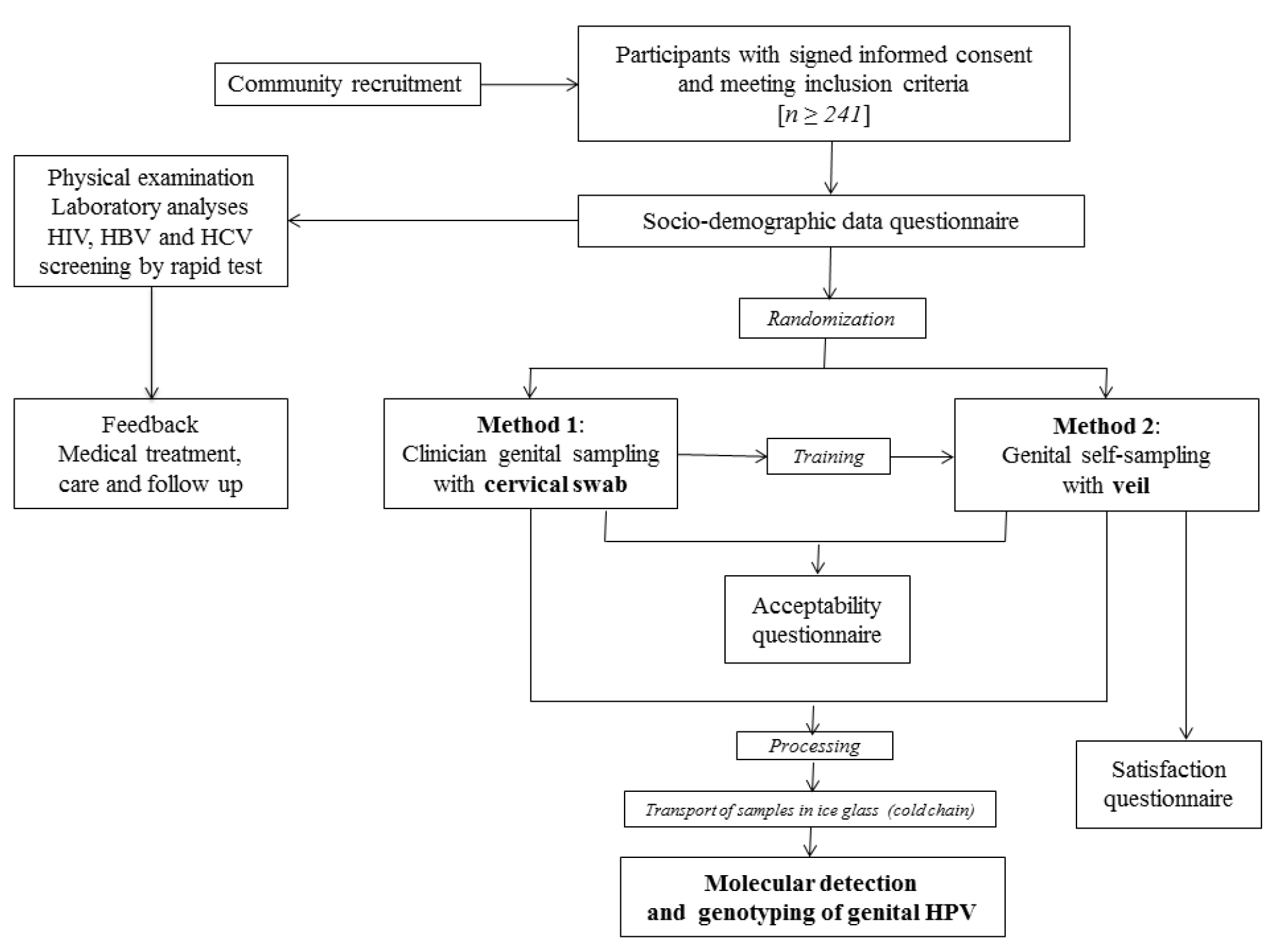
Figure 1. Flow diagram of the GYNAUTO-CHAD study. The GYNAUTO-CHAD study consisted in community-based recruitment of at least 261 adult women to be referred to the gynecologic clinic “La Renaissance Plus”, N’Djamena, Chad. The participants meeting the inclusion criteria were subjected to physical examination and care when needed, and tested for 3 chronic viral infections endemic in Chad (HIV, HBV and HCV) by capillary-based immunochromatographic rapid test, and filled in the face-to-face socio-demographic questionnaire. Afterwards, the participants were trained for self-sampling collection using the V-Veil-Up Gyn Collection Device (V-Veil-Up Pharma Ltd.) and randomly submitted to the sampling procedure with Method 1 (clinician-based collection of cervical secretions by swab, as gold standard) followed by the Method 2 (self-collection by veil) or inversely. The acceptability and satisfaction questionnaire were then administrated to the study women and collected samples were processed before molecular detection and genotyping of genital HPV infection.

For the self-collection Method 2, the study participant firstly received from a nurse a 15-minutes training on how to use the V-Veil-Up Gyn Collection Device for vaginal self-sampling, as previously reported [45]. After instructing the participant, the nurse leaved the sampling room and the participant then performed herself the self-sampling, without any help from the nurse. The participant followed the instructions for use of the V-Veil-Up Gyn Collection Device. Briefly, the study woman inserted the veil into her vagina, leaved it in-place for one hour; then removed it with the string, and returned it to the nurse. The study nurse did not witness veil insertion and removal. The nurse placed the veil impregnated with genital secretions into the dedicated collection box and closed it correctly with the cap. The veil collection box consisted of a 15 mL plastic box that contained 10 mL of phosphate-buffered saline (PBS) solution to prevent drying of the sample. The nurse verified that the PBS buffer completely submerged the veil and checked that the identification number in the label on the collection box corresponded effectively to the participant. The veil in its box was then placed in the cold (ice pack). After returning the veil specimen, a second nurse administered acceptability and satisfaction questionnaires on the woman’s experiences about the pelvic examination and clinician-based collection and the veil-based self-collection. To minimize bias, the study nurse who performed the pelvic examination was in another room and did not participate in the post-test questionnaire administration. The objectives of the acceptability questionnaire was to evaluate the study women’s experiences related to the perception of care, comfort, privacy, embarrassment, or pain associated to each collection method. The satisfaction questionnaire consisted in questions regarding the ability to understand the instructions for use of the V-Veil-Up Gyn Collection Device and its component and to perform self-collection, including home collection, and also assessed difficulties encountered during veil-collection.

Genital samples processing

Each genital sample was transported in ice packs within an hour after collection to be stored at -80°C at the virology laboratory of the hôpital Général de Référence Nationale, N’Djamena, Chad. Swabs and veils were further transported in frozen ice packs to the virology laboratory of the hôpital Européen Georges Pompidou, Paris, France, for molecular analyses.

Nucleic acid extraction

DNA was extracted from the tip of swab specimens using the DNeasyBlood and Tissue kit (Qiagen, Hilden, Germany), as recommended by the manufacturer. After extraction, DNA was concentrated in 100 μL of the elution buffer provided in the extraction kit and stored at -80°C before HPV DNA detection and genotyping, as described previously [51]. Veil samples soaked with genital secretions within PBS buffer were carefully removed from their collection box and placed into a syringe to be drained by pulling the syringe’s plunger into a 15 mL tube. The whole genital secretions were then vigorously vortexed to homogenize the fluids and finally aliquoted in 1.5 mL cryotubes (Eppendorf, Hambourg, Germany) and store at -80°C before the nucleic acid extraction procedure. In order to avoid any contamination between different specimens, the working area was sterilized between the processing of each specimen and all the consumables including gloves, syringe, forceps were for single use and were immediately discarded together with the box container. Finally, the nucleic acid extraction procedure was carried out with the DNeasy Blood and Tissue kit (Qiagen), in 1 mL of the concentrated cervicovaginal veil-collected specimen and extracted DNA was placed in 100 μL of the elution buffer provided in the extraction kit and stored at -80°C before HPV DNA detection and genotyping.

HPV detection and genotyping

HPV detection and genotyping was performed on both the clinician- and self- collected specimens using the CE IVD-marked multiplex real-time PCR assay Anyplex™ II HPV28 (Seegene, Seoul, South Korea), as described previously [52]. The kit contains specific primers targeting 28 HPV, and is based on Seegene’s proprietary DPO™ and MuDT™ technologies [53], which allow to avoid mismatch priming and to quantify each target in a single fluorescence channel, respectively. According to the HPV classification nomenclature provided by the International Agency for Research on Cancer (IARC) [54] Anyplex™ II HPV28 technology allows to detect 28 HPV genotypes in a single specimen, including 13 high-risk types (HR-HPV -16, -18, -31, -33, -35, -39, -45, -51, -52, -56, -58, -59, and -68), 9 low-risk (LR) types (LR-HPV -6, -11, -40, -42, -43, -44,-53, -54 and -70) and then, 6 genotypes classified as possibly carcinogenic (HPV-26, -61, -66, -69, -73 and -82). Briefly, 5µL of swab- or veil- extracted DNA were added into two reaction mixtures (20 µL) containing each other, one of the primers sets A and B [52]. The DNA amplification and the genotyping process were carried out in 2 reactions performed on the CFX96™ real-time PCR instrument (Bio-Rad, Marnes-la-Coquette, France) [52]. The Anyplex™ II HPV28 genotyping test has been found to be suitable for HPV detection and genotyping in cervical secretions [52, 55–58]. Data recording and interpretation were automated with Seegene viewer software (Seegene), according to the manufacturer’s instructions. A sample was considered positive for any HPV if containing any of the 28 types targeted by the Anyplex™ II HPV28 detection test; positive for multiple HPV when containing at least 2 types of the 28 HPV types included in genotypic test; HR-HPV positive and multiple HR-HPV positive when containing respectively at least 1 HR-HPV type and at least 2 high-risk types belonging to the 13 high-risk types targeted by the Anyplex™ II HPV28 detection test, irrespective of the presence of LR-HPV. The virology laboratory was accredited in 2013 by the Comité Français d’Accréditation (COFRAC) according to the ISO 15189 norma for the biological markers “HPV detection” and “HPV genotyping”.

Sample size

We hypothesized that Method 2 (self-sampling) would be non-inferior to Method 1 (flocked swab as gold standard), with a tolerated difference of Δ in the detection rate of HPV infections by molecular analysis between the two methods of collection. The requested minimum number (n) of subject to include was obtained by using Epi Info version 3.5.4 (CDC, Atlanta, USA), and by setting 95% confidence level, 80% statistical power, and considering estimated HPV prevalence of two methods in Chad. There are no data on the prevalence of genital HPV infections among women living in the Chad. In order to estimate the HPV DNA positivity in our study population, we used prevalences of genital HPV detection from comparable populations of women living in other Central African countries previously published in the literature, including 12.5% in Democratic Republic of the Congo [59], 18.5% and 34.0% in Cameroon [60, 61], and 22.2% in Rwanda [62]. Based on this assumption, we estimated the mean prevalence (P1) of HPV DNA test results to be 21.7% in the clinician-collected arm. We conducted a non-inferiority comparison with the hypothesis that the difference in HPV DNA positivity between the veil-based self-collection and clinician-collection methods would be less than 10%. With Δ of 10%, the requested minimum number (n) of subject to include was at least 241 participants.

Statistical analyses

Data was entered into an Excel database and analyzed using IBM® SPSS® Statistics 20 software (IBM, SPSS Inc, Armonk, New York, USA). Means and standard deviations (SD) were calculated for quantitative variables and proportions for categorical variables. The results were presented along with their 95% confidence interval (CI) using the Wilson score bounds for categorical variables. The overall prevalences of HPV DNA detection [any genotypes, HR-genotypes and HPV genotypes targeted by the 9-valent Gardasil-9® vaccine (Merck & Co. Inc., New Jersey, USA)] between the two collection methods were compared using the Mac Nemar’s test for paired data. The Wilcoxon’s test of paired data was used for comparison of the mean notes according to the Likert scale of acceptability of the two methods (veil-based self-collection versus swab-based clinician-collection). The agreement between the two collection methods was estimated by Cohen’s κ coefficient, and the degree of agreement was determined as ranked by Landlis and Koch [63]. Percent agreement corresponded to the observed proportion of identical results between veil-based self-collection compared to swab-based clinician-collection. Note that the acceptability of the clinician-based collection by swab and that of the veil self-collection were assessed using an arbitrary quantitative Likert scale [64] based on four different scale ranging from 1 (most difficult), 2 (difficult), 3 (easy) to 4 (= very easy or comfortable). Similarly, the satisfaction regarding the veil self-collection method was assessed using another arbitrary quantitative Likert scale based on four different scale ranging from 1 (less favorable), 2 (moderately favorable), 3 (favorable) to 4 (= most favorable). The mean and standard deviation for Likert scale data were calculated for each acceptability and satisfaction item using face-to-face questionnaires. The clinician-collected HPV DNA test results were used as the reference standard to estimate the sensitivity and specificity, with corresponding 95%CI, of the veil-collection method.

Results

Characteristics of study population

A total of 271 women from the 23 inclusion sites accepted to participate to the study, as previously reported [41,45] (Figure 2). After physical examination, 18 women were excluded because of genital troubles (vaginal discharge: 5; suspicion of STI: 3; genital bleeding: 5; sexual intercourse less than 2 days: 5). Finally, a total of 253 women (mean age, 35.0 years; range, 25–65) referred to the clinic “La Renaissance Plus” were consecutively and prospectively included in the study. Their socio-demographic characteristics, past history of STIs, sexual behavior, contraception and practices of feminine hygiene during menstruation and genital toilet have previously reported [45]. Using multiplex HIV/HCV/HBsAg rapid test, 9 study women (3.5%; 95% CI: 1.3–5.8) were infected by HIV-1, 19 (7.5%; 95% CI: 4.3–10.8) by HBV (positivity for HBsAg) and 8 (3.2%; 95% CI: 1.1–5.3) were seropositive for HCV. Most women (31.6%; 95% CI: 25.9–37.4) were young, aged from 25 to 29 years, engaged in life couple with a male partner (78.3%; 95% CI: 73.2–83.3), with a relatively high education level (32.1%; 95% CI: 26.3–37.7 and 30.4%; 95% CI: 24.7–36.1, in high school level and university, respectively); but most of them were unemployed (54.2%; 95% CI: 48.1–60.3). The majority of study women (82.2%; 95% CI: 77.5–86.9) reported having only one regular sexual partner in their life, while about 20% reported to have had up to 5 different sexual partners. Generally, the study women began sexual activity at 16 to 20 years (56.2%; 95% CI: 50.1–62.3), whereas some of them (13.8%; 95% CI: 9.6–18.1) started their sexual life earlier, before the age of 16 years. The vast majority of women (74.4%) did not take any birth control methods. Concerning the feminine hygiene during menstruation, most women (90.3%) were using sanitary napkins, while a minority (13.0%) used commercially available tampons. Genital (vulva or vagina) toilet was the rule, including post-coital toilet with water and finger in 90.3%. Finally, none of the women included in the GYNAUTO-CHAD study had ever been screened for cervical cancer and nor vaccinated against HPV infection.

JCRM-2019_Bélec Laurent_F2

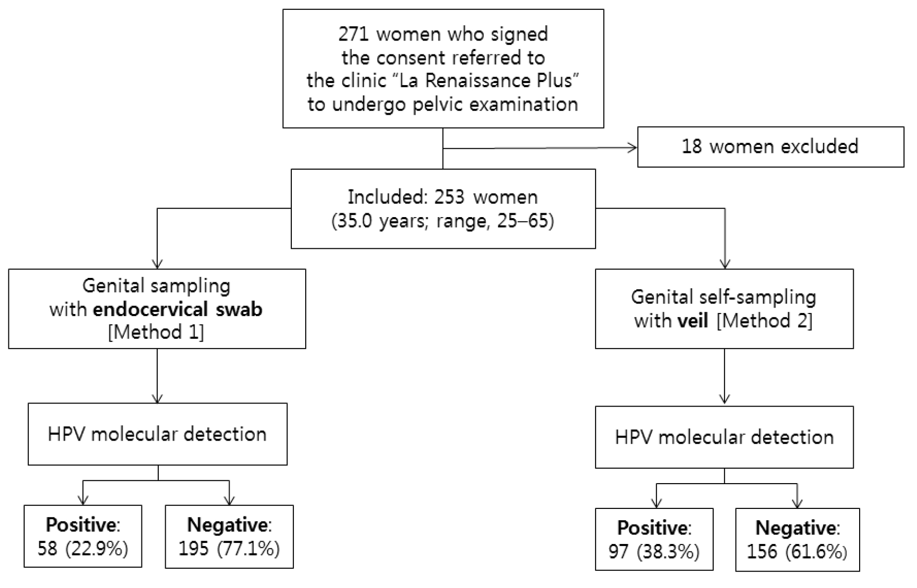
Figure 2. Flow diagram of study recruitment, specimen collection, and HPV test results by multiplex real-time PCR.

Acceptability of collection methods

Participants reported feeling much better cared for during the veil-based self-collection (mean note of 3.1 according to the Likert scale of acceptability) compared to swab-based clinician-collection (mean note of 1.4; P < 0.02) and also more in privacy handled during self-collection (mean note of 3.1) compared to clinician-collection (mean note of 1.4; P < 0.005) (Table 1). There were no other significant differences in embarrassment, discomfort or genital pain between the two collection methods (Table 1). When asked to choose one collection method, 243 (96.0%) of study women responded that they would prefer the self-collection method. Furthermore, most participants (237; 89.7%) reported that they would be willing to perform veil-collection at home and bring the specimen with them to clinic.

Table 1. Acceptability of veil-based self-sampling using the V-Veil-Up Gyn Collection Device (V-Veil-Up Pharma Ltd.) compared to swab-based clinician-collection for HPV DNA testing among 253 study women living in N’Djamena, Chad.

Acceptability items*

Veil-based self-collection [mean (SD)]

Swab-based clinician-collection [mean (SD)]

P-value**

How well cared for did you feel?

3.1 (0.8)

1.4 (0.5)

0.011

How well was your privacy handled during the test?

3.1 (0.5)

1.4 (0.5)

0.003

Did you feel embarrassed?

3.3 (1.2)

3.1 (1.4)

0.835

Did the test cause you any genital discomfort?

3.1 (1.3)

3.1 (1.2)

1.000

Did the test cause you any genital pain?

2.9 (1.4)

2.5 (1.4)

0.700

* The scale of acceptability was assessed by a Likert scale ranging from 1 (most difficult) to 4 (= most favorable); the results are mean ± 1 standard deviation (SD);

** Statistical comparisons were assessed by Wilcoxon’s test for paired data.

Satisfaction of self-sampling using the V-Veil-Up Gyn Collection Device

The results of the face-to-face satisfaction questionnaire regarding veil-based self-sampling using the V-Veil-Up Gyn Collection Device are shown in the Table 2. In addition, most women (231; 91.3%) reported that the instructions for use written in French were easy to read and to understand, while the verbal explanations on how to use the collection device showed higher mean note according to the Likert scale of satisfaction (written versus oral explanation: 2.9/4 and 3.6/4, respectively). A significant number of participants (76; 30.0%) reported difficulties in correctly interpreting schemas. The large majority of women (245; 96.8%) were able to recognize correctly the component’s device, with high notes (3.6/4). In addition, the veil was generally (243; 97.6%) correctly placed with the applicator and removed with the string. Difficulties on understanding how to place the veil deep within the vaginal cavity were frequently encountered in one-third of participants (86; 33.9%) with a low mean note of 0.9/4. All items concerning the general satisfaction of the V-Veil-Up Gyn Collection Device showed high mean notes from 2.9 to 3.3. Discomfort when carrying the veil concerned only urges to urinate. Genital pain when placing or wearing the veil was reported in a minority of women (10; 3.9%), all being more than 45 years-old. Finally, only 12 (4.7%) women reported some difficulties with performing the self-collection.

Table 2. Satisfaction questionnaire regarding veil-based self-sampling using the V-Veil-Up Gyn Collection Device (V-Veil-Up Pharma Ltd.) among 253 study women living in N’Djamena, Chad.

Variables*

Veil-based

self-collection

[mean (SD)]

95%CI

Understanding of instruction for use

Instruction for use in French language

2.9 (1.1)

[2.7-3.0]

Verbal explanation of instruction for use

3.6 (0.5)

[3.5-3.7]

Anatomic sketches

2.4 (1.1)

[2.2-2.5]

Understanding of component’s device

Device has three components (veil ; applicator and string)

3.6 (0.4)

[3.6-3.7]

Veil includes pocket for drug or cream

3.6 (0.5)

[3.6-3.7]

Correct use of the veil

Applicator to be placed in the pocket

3.7 (0.5)

[3.6-3.7]

String to be used to remove the veil after use

3.8 (0.4)

[3.8-3.7]

Place the veil deep within the vaginal cavity

0.9 (0.1)

[0.9-1.0]

General satisfaction

Keeping the veil into the vagina for 60 minutes

3.1 (0.8)

[3.0-3.2]

Removing the veil impregnated with genital secretions with the string

3.3 (0.7)

[3.2-3.4]

Comfort when carrying the veil

3.3 (1.2)

[3.2-3.5]

Genital pain when placing or wearing the veil

2.9 (1.4)

[2.7-3.1]

General opinion about veil-based self-sampling

3.1 (0.5)

[3.0-3.1]

* The scale of satisfaction was asses by a Likert scale ranging from 1 (= less favorable) to 4 (= most favorable); the results are mean ± 1 standard deviation (SD); 95% confidence intervals (CI) are given in brackets.

Prevalences of HPV detection and genotypes distribution by collection methods

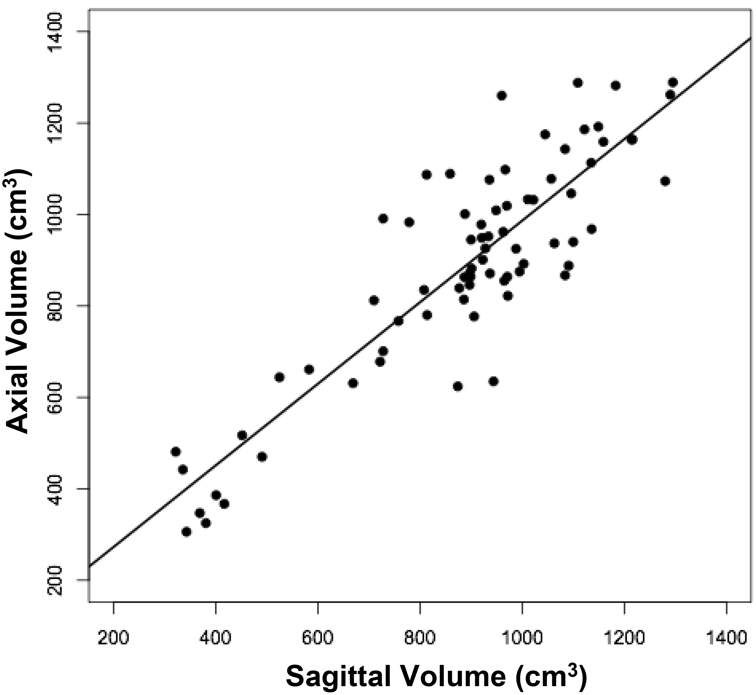
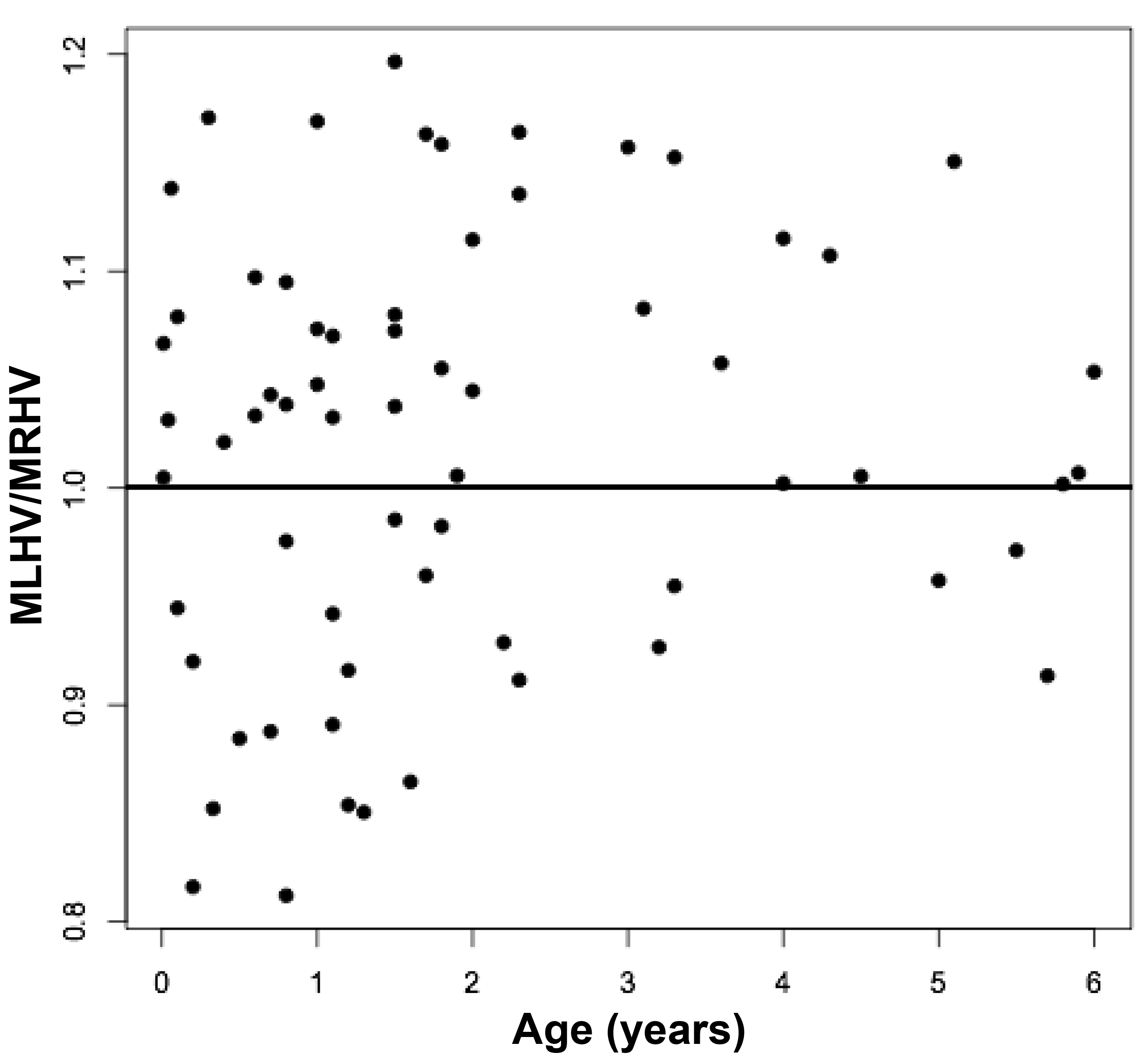
All 253 study participants had paired clinician-collected and self-collected specimens obtained for laboratory testing. All secretions from swab and veil specimens were positive for the ubiquitous b-globin gene, used as internal control of cell sampling of the Anyplex™ II HPV28 kit. Results from each of the collection method are presented in Tables 3, 4, 5 and 6 and in Figures 3, 4 and 5. Of the clinician-collected specimens included in the analysis, 58 women were positive for genital HPV DNA giving a total HPV prevalence of 22.9% (95% CI: 17.8–28.1), with 68.9% (40/58; 95% CI: 57.1–80.8) harboring cervical HR-HPV infection, providing a total HR-HPV prevalence of 15.8% (95% CI%: 11.3–20.3), as shown in the Table 3. The whole distribution of HPV genotypes in HPV-DNA positive cervical samples is detailed in the Figure 3. The Gardasil-9® vaccine HR-HPV type 58 was the predominant genotype (7/58; 12.1%), followed by the HR-HPV types 31, 35 and 56 and the LR-HPV types 42 and 44 with a prevalence of 10.3% (6/58). The 9-valent vaccine HR-HPV types 16, 45 and 52 and also the LR-HPV types 53 and 70 were present [prevalence of 8.6% (5/58)]. These HPV genotypes were followed by the HR-HPV types 18 and 51, 59 and 68 and the LR-HPV types 6 and 54 and finally the possibly oncogenic HPV types 73 and 82 with a prevalence of 6.8% (4/58). The HR-HPV-39 was present only in 3 women (5.2%) and none of the HPV positive samples was simultaneously positive for HPV-16 and HPV-18.

JCRM-2019_Bélec Laurent_F3

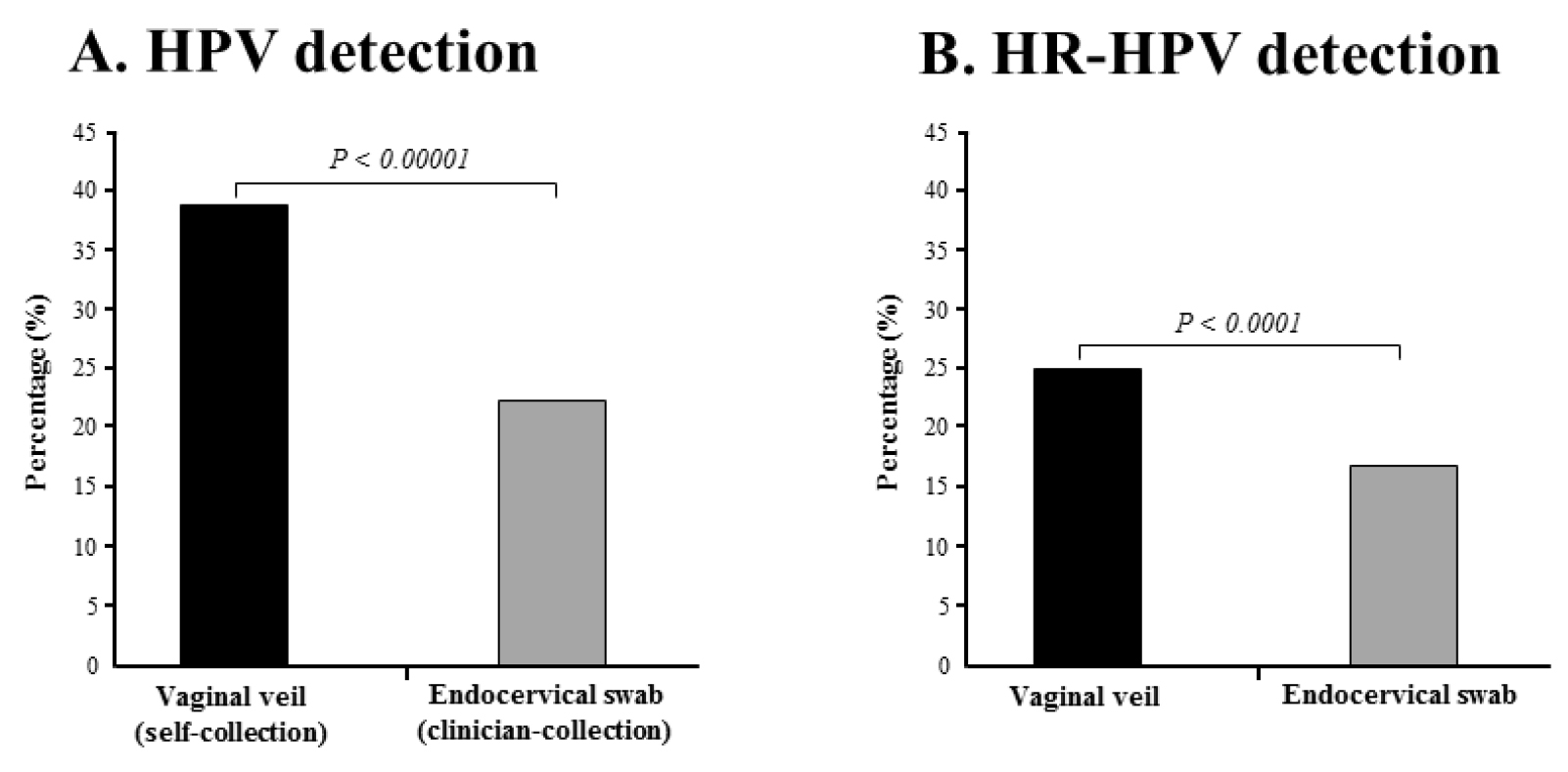
Figure 3. Percentages of detection by multiplex real-time PCR assay Anyplex™ II HPV28.
HPV DNA (A) and HR-HPV DNA (B) in paired genital secretions obtained by gold standard clinician-collected endocervical swab and by self-collection using the V-Veil-Up Gyn Collection Device (V-Veil-Up Pharma Ltd.) among 253 study women living in N’Djamena, Chad. P-values of the comparison between the two collection methods using the Mac Nemar’s test for paired data are indicate in italic.

Table 3. HPV DNA detection by clinician-collected swab and by self-collected veil among the 253 study adult women living in N’Djamena, in Chad, and included in GYNAUTO-TCHAD study.

Study women
(N=253)

Characteristics

n (%) [95%CI]*

HPV DNA detection using endocervical swab**

HPV DNA

58 (22.9) [17.8-28.1]

HR-HPV DNA

40 (15.8) [11.3-20.3]

Multiple types of any HPV among HPV-positive swabs

16 (27.6) [16.1–39.1]

Multiple types of HR-HPV among HR-HPV-positive swabs

10 (25.0) [11.6–38.4]

Any 9-valent vaccine types*** among HPV-positive swabs

29 (50.0) [37.1–62.9]

9-valent vaccine HR-HPV types among HR-HPV-positive swabs

27 (67.5) [52.9–82.1]

HPV DNA detection using self-collected veil****

HR-HPV DNA

97 (38.3) [32.4-44.3]

HR-HPV DNA

63 (24.9) [19.6-30.2]

Multiple types of any HPV among HPV-positive veils

42 (43.3) [33.4–53.2]

Multiple types of HR-HPV among HR-HPV-positive veils

16 (25.4) [14.6–36.2]

Any 9-valent vaccine types*** among HPV-positive veils

48 (49.5) [39.5–59.4]

9-valent vaccine HR-HPV types among HR-HPV-positive veils

43 (68.3) [56.8–79.7]

* The frequency of each variable is presented with their 95% confidence interval in brackets;

** HPV testing using endocervical secretions obtained by clinician-collected flocked swab;

*** The 9-valent Gardasil-9® vaccine (Merck & Co. Inc.) is effective against HPV genotypes 6, 11, 16, 18, 31, 33, 45, 52 and 58;

**** HPV testing using cervicovaginal fluid collected from self-administered veil (V-Veil-Up Gyn Collection Device, V-Veil-Up Pharma Ltd.) introduced within the vaginal canal during 60 minutes.

95%CI: 95% confidence interval; HBV: Hepatitis B virus; HCV: Hepatitis C virus; HIV: Human immunodeficiency virus; STI: Sexual transmitted infection; HPV: Human papillomavirus; HR-HPV: High-risk human papillomavirus: SD: Standard deviation.

Of the veil-based self-collected specimens included in the analysis, 97 women showed genital shedding of HPV DNA that represented an overall HPV prevalence of 38.3% (95% CI: 32.4–44.3). Among these HPV positive women, 64.9% [(63/97); 95% CI: 55.45–74.4] were positive for HR-HPV genotypes giving a total HR-HPV prevalence of 24.9% (95% CI: 19.6–30.2) (Table 3). The whole distribution of HPV genotypes in HPV-DNA positive cervical samples collected by veil is detailed in the Figure 3. The distribution of HPV genotypes in the HPV DNA-positive women revealed that the LR-HPV genotype 42 (13/97; 13.4%) was the predominant genotype, followed by the HPV54 (12/97; 12.4%), HPV70 (11/97; 11.3%). The Gardasil-9® vaccine HR-HPV type 58, 52 and 31 were the predominant HR-HPV genotypes (9/97; 9.3%), followed by HPV16 (8/97; 8.2%), HPV18, HPV35, HPV45 and HPV68 (7/97; 7.2%), HPV39 (5/97; 5.2%) and finally HPV33 (2/97; 2.1%). The percent agreements between the two collection methods to detect any HPV, HR-HPV and 9-valent vaccine HPV genotypes were 83.0%, 89.3% and 91.7%, respectively, and all Cohen’s κ coefficients were between 0.61 to 0.80, demonstrating “good” agreement [56] (Table 4).

Table 4. Two-by-two tables of cervicovaginal specimens self-collected using the V-Veil-Up Gyn Collection Device (V-Veil-Up Pharma Ltd.) compared to clinician-collected endocervical swab specimens for the detection by multiplex real-time PCR of any HPV genotypes, HR-HPV genotypes and HPV genotypes targeted by the 9-valent Gardasil-9® vaccine (Merck & Co. Inc.).

Any HPV genotypes

HR-HPV
genotypes

9-valent vaccine HPV genotypes

Clinician-collected
swab specimen

Clinician-collected
swab specimen

Clinician-collected
swab specimen

Positive
(n=58)

Negative
(n=195)

Positive
(n=40)

Negative
(n=213)

Positive
(n=29)

Negative
(n=224)

Veil-based self-collected specimen

Positive
(N*=97)

56

41

Positive
(N***=63)

38

25

Positive
(N$=48)

28

20

Negative
(N**=156)

2

154

Negative
(N****=190)

2

188

Negative
(N£=205)

1

204

Estimate

95% CI

Estimate

95% CI

Estimate

95% CI

Sensitivity (%)

96.5

91.8–100.0

95.0

88.3–100.0

96.5

89.8–100.0

Specificity (%)

78.9

73.3–84.7

88.2

83.9–92.6

91.1

87.3–94.8

Agreement (%)

83.0%

89.3%

91.7%

Cohen’s κ coefficientµ

0.611

0.675

0.682

* : Total number of veil based-self collected specimens positive for any HPV;

** : Total number of based-self collected specimens negative for any HPV;

*** : Total number of veil based-self collected specimens positive for HR-HPV;

**** : Total number of veil based-self collected specimens negative for HR-HPV;

$ : Total number of veil based-self collected specimens positive for any HPV genotypes targeted by the 9-valent Gardasil-9® vaccine (Merck & Co. Inc.) (HPV -6, -11, -16, -18, -31, -33, -45, -52 and -58);

£ : Total number of veil based-self collected specimens negative for any HPV genotypes targeted by the 9-valent Gardasil-9® vaccine;

µ : The Cohen’s k coefficient was interpreted according the Landis and Koch scale [56]: For k value 0, the agreement is considered to be less than what would be expected by chance; for º values 0.01 0.20, only a slight agreement is present; for º values 0.21 0.40, the agreement is considered to be fair; for º values 0.41 0.60, the agreement is said to be moderate; for º values 0.61 0.80, the agreement is considered good; and finally, for º values 0.81 0.99, the agreement is said to be almost perfect.

HPV: Human papillomavirus; HR-HPV: high-risk human papillomavirus.

Using clinician-collected swab as the reference collection method, the sensitivities and specificities of the self-collected veil to detect HPV, HR-HPV and 9-valent vaccine HPV genotypes were 96.5% (95% CI: 91.8 – 100.0%) and 78.9% (95% CI: 73.3 – 84.7%), 95.0% (95% CI: 88.3 – 100.0%) and 88.2% (95% CI: 83.9 – 92.6%), and 96.5% (95% CI: 89.8 – 100.0%) and 91.1% (95% CI: 87.3 – 94.8%), respectively (Table 4). Overall, the percentage of test positivity for HPV DNA was 1.67-fold higher in self-collected specimens than in clinician-collected specimens (38.3% versus 22.9%; P-value < 0.00001) (Figure 3A). The percentage of test positivity for HR-HPV DNA was 1.57-fold higher in self-collected specimens than in clinician-collected specimens (24.9% versus 15.8%; P-value < 0.0001) (Figure 3B). When considering the distribution of the 28 HPV genotypes detected by multiplex real-time PCR assay Anyplex™ II HPV28 detected in paired genital specimens, all genotypes but two (HPV-59 and HPV-82), were more frequently detected by self-collection using the V-Veil-Up Gyn Collection Device than by clinician-collected endocervical swab (Figure 4).

JCRM-2019_Bélec Laurent_F4

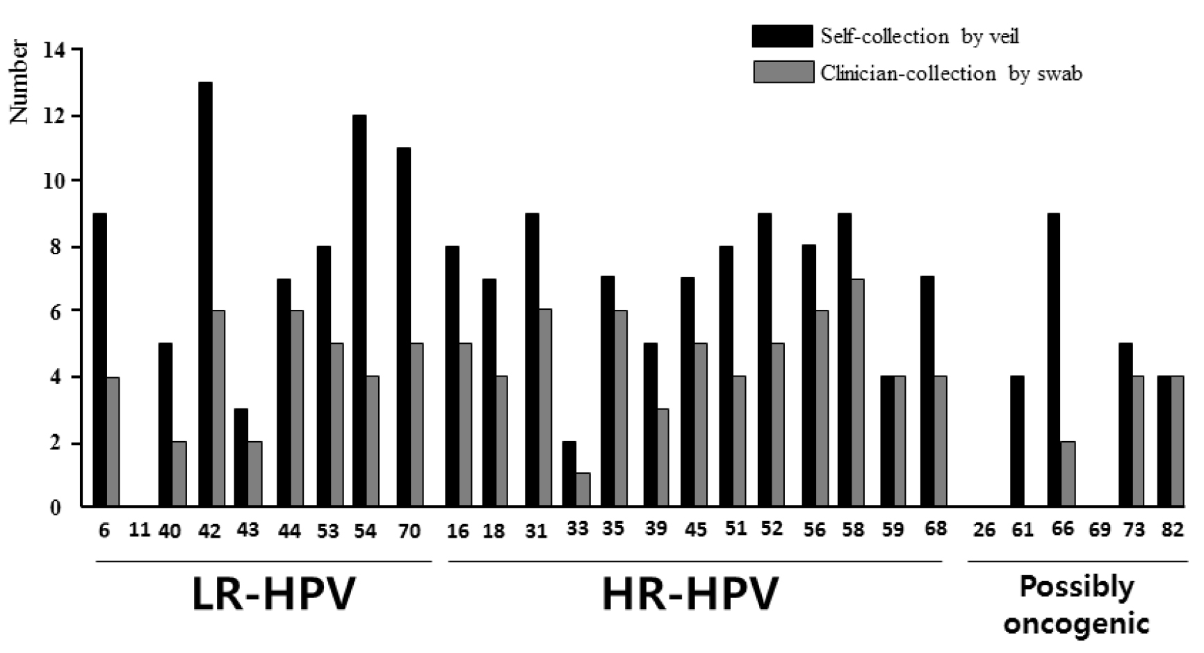
Figure 4. Distribution of the 28 HPV genotypes detected by multiplex real-time PCR assay Anyplex™ II HPV28.
The HPV DNA detection was carried out in paired genital secretions obtained by clinician-collected endocervical swab and by self-collection using the V-Veil-Up Gyn Collection Device (V-Veil-Up Pharma Ltd.) among 253 study women living in N’Djamena, Chad. LR-HPV: Low risk- human papillomavirus; HR-HPV: High-risk human papillomavirus.
The 28 HPV genotypes detected by the Anyplex™ II HPV28 kit include 9 low-risk types (LR-HPV), 13 high-risk types (HR-HPV) and 6 genotypes classified as possibly carcinogenic. The HPV genotypes -6, -11, -16, -18, -31, -33, -45, -52 and -58 which are targeted by the 9-valent Gardasil-9® vaccine (Merck & Co. Inc.) are highlighted in grey.

Among the 253 study participants, the mean numbers (± 1 SD) of HPV and HR-HPV detected when using the self-collected veil [1.84±0.96 (range, 1–10) and 1.43±0.64 (range, 1–5), respectively] were similar to those obtained when using the swab-collection [1.79±1.14 (range, 1–9) and 1.5±0.75 (range: 1–5), respectively]. The differential efficiency of detecting HPV and HR-HPV between the two collection methods was better evidenced when considering paired results by genotype. Thus, the correspondence between the 7,084 (=253 x 28) results obtained from the 253 paired swab-collected and veil-collected genital specimens to detect the 28 HPV genotypes included in Anyplex™ II HPV28 kit was further analyzed, genotype by genotype, and depicted in Table 5. The use of self-collection by veil allowed detecting 101 (84+17) additional HPV of all types by reference to the use of swab in 89 (35.2%) participants, while the use of swab allowed detecting only 7 additional HPV in 7 participants (2.8%) by comparison to the use of veil. When considering only the correspondence between the 3,289 (=253 × 13) paired results for oncogenic HR-HPV (Table 6), the use of veil allowed detecting 38 (34+4) additional HR-HPV in 35 (13.8%) study women, while the use of swab allowed detecting only 3 additional HPV in 3 participants (1.2%) by comparison to the use of veil. The Figure 5 depicts some relevant examples of paired results obtained by clinician-collected endocervical swab and self-collected veil using the multiplex real-time PCR assay Anyplex™ II HPV28, showing the capacity of the veil to allow the detection of oncogenic HR-HPV that could not be detected from the paired swab specimens. Finally, genital infections with multiple HPV genotypes were more frequently detected using the veil collection device than swab collection [43.3% (42/97); 95% CI: 33.4–53.2 versus 27.6% (16/58); 95% CI: 16.1–39.1; P < 0.001], while the mean number of HR-HPV detected using positive genital secretions collected by veil was quite similar to that of cervical secretions collected by swab [1.7 HR-HPV genotypes (range, 1 to 5) versus 2.3 HR-HPV (range, 1 to 5)].

Table 5. Correspondence between the 7,084 (= 253 × 28) results obtained from the 253 paired swab-collected and veil-collected genital specimens to detect the 28 HPV genotypes included in Anyplex™ II HPV28 kit (Seegene).

LR-HPV

HR-HPV

Possibly oncogenic

6

11

40

42

43

44

53

54

70

16

18

31

33

35

39

45

51

52

56

58

59

68

26

61

66

69

73

82

Swab

Veil

Number of cases per genotype

Total

Negative

Negative

244

253

248

240

248

244

245

241

242

244

246

244

250

246

248

246

245

244

244

244

249

245

253

249

244

253

248

249

6,891

Positive

Positive with same genotype*

4

0

2

6

0

4

5

4

5

4

4

6

0

6

3

5

4

5

6

7

4

3

0

0

2

0

4

4

97

Positive

Positive with different genotypes **,a

0

0

0

0

1b

2c

0

0

0

0

0

0

1d

0

0

0

0

0

0

0

0

0

0

0

0

0

0

0

4

Negative

Positive

5

0

3

7

3

3

3

8

6

4

3

3

2

1

2

2

4

4

3

2

0

4

0

4

7

0

1

0

84

Positive

Negative

0

0

0

0

2

2

0

0

0

1

0

0

1

0

0

0

0

0

0

0

0

1

0

0

0

0

0

0

7

* i.e., positivity using veil for the same HR-HPV genotype using swab;

** i.e., positivity using veil for at least one another HR-HPV genotype using swab;

a A total of 17 additional HPV genotypes were detected using veil collection;

b Additional HPV genotypes detected using veil collection were HPV -16, -52, -53, -54, -70 and -73;

c Additional HPV genotypes detected using veil collection were HPV -43 and -54;

d Additional HPV genotypes detected using veil collection were HPV -6, -31, -43, -51, -54, -59, -66, -68 and -66.

NA: Not attributable; HPV: Human papillomavirus; HR-HPV: high-risk human papillomavirus; LR-HPV: low-risk human papillomavirus.

JCRM-2019_Bélec Laurent_F5

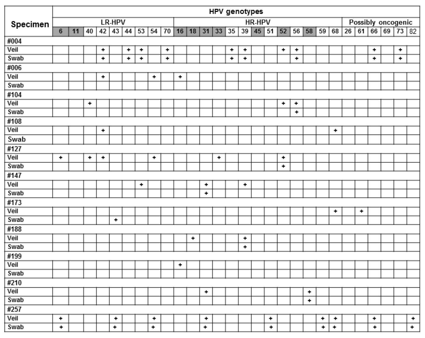
Figure 5. Relevant examples of paired results obtained by gold standard clinician-collected endocervical swab and self-collected veil.
Participants #006, #108, #199 and #257 were negative by clinician-collected swab, whereas they were positive by paired self-collected veil, with supplementary detection by veil of oncogenic HR-HPV, including HPV-16 in #006 and #199, HPV-68 in #108, and HPV-31, HPV-51 and HPV-68 in #257. Participants #004, #104, #127, #147, #173, #188 and #210 were positive by clinician-collected swab, and paired self-collected veil allowed supplementary detection of several oncogenic HR-HPV (HPV-18 in #188; HPV-31 in #210; HPV-33 in #127, HPV-39 in #147, HPV-52 in #004 and #104; HPV-68 in #173). Interestingly, all positive HR-HPV detections by clinician-collected swab were also detected by self-collected veil. Positive result for a given genotype is indicated by cross; negative result by white box. All swab and veil specimen were positive for b-globin internal control of the Anyplex™ II HPV28 kit (not shown).

Table 6. Correspondence between the 3,289 (= 253 × 13) results obtained from the 253 paired swab-collected and veil-collected genital specimens to detect the 13 HR-HPV genotypes included in Anyplex™ II HPV28 kit (Seegene).

HR-HPV genotypes

16

18

31

33

35

39

45

51

52

56

58

59

68

Swab

Veil

Number of cases per genotype

Total

Negative

Negative

244

246

244

250

246

248

246

245

244

244

244

249

245

3,195

Positive

Positive with same genotype*

4

4

6

0

6

3

5

4

5

6

7

4

3

57

Positive

Positive with different genotypes**,a

0

0

0

1b

0

0

0

0

0

0

0

0

0

1

Negative

Positive

4

3

3

2

1

2

2

4

4

3

2

0

4

34

Positive

Negative

1

0

0

1

0

0

0

0

0

0

0

0

1

3

* i.e., positivity using veil for the same HR-HPV genotype using swab;

** i.e., positivity using veil for at least one another HR-HPV genotype using swab;

a A total of 4 additional HR-HPV genotypes were detected using veil collection;

b Additional HR-HPV genotype detected using veil collection was HR-HPV -31, -51, -59 and -68.

NA: Not attributable; HPV: Human papillomavirus; HR-HPV: high-risk human papillomavirus.

Discussion

In the present study, the acceptability and HPV DNA diagnostic accuracy of a novel genital veil (V-Veil-Up Gyn Collection Device) was assessed as female genital self-sampling device to collect cervicovaginal secretions. Interestingly, all specimens collected by the veil were found positive for the ubiquitous b-globin gene, demonstrating that they contained cellular DNA, which made HPV detection possible by molecular testing. The results showed high acceptability (96%), feasibility and satisfaction of the veil-based genital self-collection, which was non-inferior to clinician-based collection as reference for HPV DNA molecular testing, with “good” agreement between the two collection methods, high sensitivity of 95.0% and specificity of 88.2%. Outstandingly, the rates of HPV DNA and HR-HPV DNA positivities were significantly higher when using veil-based collected genital secretions than clinician-collected cervical secretions by swab. The self-collection by veil allows detecting 12.7-fold more additional oncogenic HR-HPV in 1 of 8 (12.5%) participants than the detection allowed by the swab-based collection, likely originating from non-cervical areas of the vaginal cavity, including vaginal cul-de-sacs, vaginal walls and vulva. Taken together, our observations highlight that veil-based self-collection of genital secretions appears a convenient tool to collect in a gentle way genital secretions for accurate molecular HPV detection and genotyping that could be easily implemented in the cervical cancer prevention program in Chad.

Most previous studies conducted in sub-Saharan African countries depict high HR-HPV prevalences and wide heterogeneity in the distribution of the main HR-HPV in women [59–62, 65–79]. Our observations confirm that women living in Chad also form a neglected high-risk group for cervical HR-HPV infection and consequently for cervical cancer. The very high prevalence of cervical HR-HPV in adult women clearly demonstrates that cervical HR-HPV infection in Chad constitutes a major public health problem, which remains largely unsuspected. Therefore, there is an urgent need for implementing a cervical cancer prevention program in Chad, as recommended by the World Health Organization (WHO) [80]. According to Mortier and colleagues, the cytology-based cervical cancer screening in women in Chad is feasible with low cost and easy to interpret visual technics; and could be integrated in existing healthcare structures [40]. For these women carrying cervical HR-HPV infection, only secondary prevention with regular screening for precancerous lesions by cytology and the monitoring of the viral persistence by HPV molecular testing, remains the only alternative to prevent the disease progression into invasive cervical cancer. However, in the context of Chad, a very low-income country, there is a serious lack of pathologist specialists, thereby making conventional cytology not suitable and reinforcing on the other hand the great necessity to implement HPV DNA testing with molecular technologies [7]. Indeed, HPV DNA testing constitutes an alternative to cytology for cervical cancer screening, which is furthermore highly sensitive and reproducible [7]. HPV DNA molecular testing could promote the “screen-and-treat” strategy recommended by the WHO to prevent cervical cancer in developing countries [80], thus allowing to maximize the medical support in a single visit and avoiding the loss of women positive for HR-HPV.

Taking into account that most adult Chadian women are living in remote rural areas, or far away of adequate healthcare facilities, self-collection of genital specimen carried out at home by women themselves could represent a relevant alternative allowing increasing the coverage of screening when coupled with adapted HPV DNA testing by molecular biology [7]. In the GYNAUTO-CHAD study, we have had the opportunity to evaluate the acceptability and HPV DNA diagnostic accuracy of a novel genital veil (V-Veil-Up Gyn Collection Device) as female genital self-sampling device to collect cervicovaginal secretions, previously found accurate for the molecular detection of cervicovaginal bacterial infections [45]. Veil-based self-collection proved to be a particularly well acceptable method easily collecting genital secretions within our cohort of community-recruited adult Chadian women. Thus, the veil was in the vast majority of participants (97.6%) correctly placed with the applicator and removed with the string, without any difficulties. When asked to choose one collection method, the vast majority (96.0%) of study women responded that they would prefer the self-collection method, demonstrating high acceptability of the genital sampling using the V-Veil-Up sampler device. Although most women (91.3%) reported that the instructions for use in French were easy to read and to understand, with correct recognizing of the component’s device, the verbal explanations by the nurse on how to use the collection device were better appreciated, particularly to correctly interpret the schemas of the instructions for use, and how placing the veil deep within the vaginal cavity. These observations are in keeping with the frequent ignorance of female genital anatomy in study participants (not shown), who were not generally taking any birth control method, and were not using tampons for feminine hygiene during menstruation. However, in practice, the manipulation of the veil was almost correct, perhaps in relationship with the very frequent usage of genital toilet in study women. Thus, while the majority of participants were not already familiar with using tampons (only 13% in our study population), the genital manipulations during veil-based self-collection were easy to carry out, which might lead to greater preference for the veil much over than other unfamiliar methods, such as a brush or a swab. These findings are reminiscent to the high acceptability of the use of vaginal tampons for self-collection reported in African women living in South Africa [13, 30]. These observations suggest that a large proportion of African women might actually prefer self-collection methods not necessitating good knowledge of the female genital anatomy to other self-collection methods such as brush or swab, for which the women must specifically target their cervix. Furthermore, the answers of study participants demonstrated high satisfaction of the V-Veil-Up Gyn Collection Device. Thus, very few women reported difficulties when performing the veil-based collection and nearly all women reported positive experiences with collection. Only a minority (4.7%) of participants reported some difficulties with performing the self-collection, most frequently genital pain when placing or wearing the veil in a minority of women (3.9%), all being more than 45 years-old, likely because of vaginal dryness in women being in the menopause period.

Otherwise, our observations also point the potential interest of using a supervised self-collection strategy among African women, in which oral counselling processes are aided at all times by a healthcare or non-healthcare professional as a counsellor to understand the instructions for use, the genital anatomy, and provide counselling with a very high rate of acceptability and satisfaction of self-collection. The evidence of high acceptability for supervised strategies was previously reported for another self-collection of capillary blood or saliva during HIV self-testing, especially in resource-constrained settings [81]. Other advantages of veil are that it is inexpensive and easily accessible. Finally, providing options for self-collection based upon women’s preferences is likely to increase screening coverage, and our data suggest that veil is an acceptable option. The percent agreements between clinician-based collection and veil-based self-collection to detect any HPV, HR-HPV and 9-valent vaccine HPV genotypes were above 80%, and all Cohen’s κ coefficients were between 0.61 to 0.80 demonstrating “good” agreement between collection methods [63]. Although it exists no data on the performance of self-collected specimens by veil for HPV DNA testing for which to compare our results, several previous reports evaluating the use of self-collection by vaginal tampons and vaginal lavages for HPV DNA or HR-HPV mRNA may be useful to contextualize our results, since tampons and lavage as well as veil do not target particularly the cervix but are the reflect of the whole secretions of the vaginal cavity [82]. Thus, our findings of agreement between the two collection methods with the kappa-statistic are relatively similar to previous reports evaluating HR-HPV DNA detection by self-collection using vaginal tampons with clinician-collection as reference, with Cohen’s κ coefficients ranging from 0.49 [83], 0.55 [84], 0.50 [12], 0.63 [49], 0.70 [85], 0.75 [84] to 0.76 [86] or vaginal lavage with Cohen’s κ coefficients ranging from 0.47 [18], 0.53 [18], 0.64 [87], 0.65 [88], 0.71 [89] to 0.78 [88], thus indicating “moderate” to “good” agreements [63]. Similarly, the performances of HR-HPV mRNA testing using self-collected vaginal tampons by reference to clinician-collected specimens, with Cohen’s κ coefficient of 0.54 indicating “moderate” agreement [30], were slightly below to the agreement of the veil.

Out of 40 HR-HPV-positive clinician-collected specimens, 38 veil-collected specimens were also positive for HR-HPV, corresponding to a sensitivity of 95.0%. Using vaginal tampon, Adamson and colleagues reported much lower sensitivity of 77.4% of vaginal tampons to detect HR-HPV mRNA by reference to clinician collection by swab [30]. A wide range of sensitivities of tampon collection using clinician-collection as the reference were reported to detect HR-HPV DNA, ranging from 59% to 94% [12, 21, 23, 84, 90–94] and always lower than the sensitivity of the veil observed in our hands. Similarly, the reported sensitivities of vaginal lavage to detect HR-HPV ranged from 88% to 90% [88]. It remains unclear whether these differences are due to different duration of collection time, different order of specimen collection, or whether they reflect the differences in testing methods. One reason for the lower sensitivity of the tampon-based collection might be due to sampling location. The clinician-collected specimen, obtained directly from the cervix, preferentially collects cervical cells in the transformation zone, whereas the tampon-method provides a mix of cells from both the cervix and vagina, and therefore might not collect enough cells from the transformation zone [82]. In contrast, the high sensitivity with the veil to detect cervical HR-HPV demonstrates that the veil likely retains significant amount cells originating from the cervix and more than a simple vaginal tampon. It is possible that extending the time of holding the veil might increase the sensitivity, but it also might lead to decreased acceptability [21]. Finally, it is important to note that the reported sensitivities of self-sampling by vaginal tampons in addition with our own sensitivity with the veil are only for molecular detection of HPV, since no pathological data were recorded to predict dysplastic or pre-invasive lesions such as CIN 2+.

Likewise, of the 213 clinician-collected specimens negative for HR-HPV DNA, 188 veil-collected specimens were also negative for HR-HPV DNA, corresponding to a specificity of 88.2%. The specificity of the veil is of the same order to those previously reported for self-collection to detect cervical HR-HPV DNA by vaginal tampons, ranging from 80% to 92% [12, 21, 84, 90, 91], but higher than that previously reported for self-collection by tampons to detect cervical HR-HPV mRNA (77.7%) [30]. The difference in sampling location between the clinician-based collection using swab targeting the endocervix and the self-collection by veil or tampons collecting global cervicovaginal secretions might explained the higher rate of positive results by veil or tampons than by swab, since the veil as well as vaginal tampons might have picked up vulvovaginal HPV infections, which do not necessarily coincide with cervical infections [82, 94].

Because clinical management and research usually depend on single-point detection of HPV, it is important to use the collection method the most capable to detect HPV by molecular biology. The cumulative presence of HPV in female genital tract is always greater than its point prevalence, suggesting that single-point sampling is less than 100% sensitive [49]. Otherwise, the vaginal epithelium represents a much greater surface area than the cervical epithelium and as such offers a greater number of potentially HPV-infected cells to collect. Thus, the self-sampling approach using veil might not only sample the cervix, but it will also sample the vaginal epithelium, with a potentially greater likelihood of detecting HPV. Indeed, vaginal epitheliums together with the cervix epithelium provides a potentially higher number of HPV-infected cells than the cervix alone. Remarkably, in the present study, the percentages of test positivity for HPV DNA and HR-HPV DNA were 1.67-fold and 1.57-fold higher, respectively, in self-collected specimens by veil than in clinician-collected specimens. Furthermore, when considering the distribution of the 28 HPV genotypes detected by multiplex real-time PCR assay Anyplex™ II HPV28 in paired genital specimens, the vast majority (92.8%) of genotypes were more frequently detected by self-collection using the V-Veil-Up Gyn Collection Device than by clinician-collected endocervical swab. In more than one-third (35.2%) of participants, the self-collection by veil allowed detecting nearly 14.4 (101/7)-fold more additional HPV (not detected by swab) than those detected using the clinician-collection by swab. Likewise, the use of veil allowed detecting 12.6 (38/3)-fold more additional HR-HPV in 1 of 8 (13.8%) participants than the use of swab. These findings suggest that the veil is able significantly releasing genital cells for HPV molecular testing, likely better than vaginal tampon. Indeed, cell clusters embedded in a rayon-covered cotton core tampon are not easily separated from the sampling device [48]. Our observations also demonstrate the high capacity of the veil to allow the detection of oncogenic HR-HPV present within the vaginal cavity that could not be detected from the paired swab specimens. Finally, the veil was more efficient to detect oncogenic HR-HPV in whole cervicovaginal secretions than the swab used to collect cervical secretions. Indeed, the veil collects all types of cervicovaginal secretions of the vaginal cavity, not exclusively the cervical secretions, and thus allows detecting non-cervical HPV. Non-cervical HPV are a priori located at non-cervical vaginal areas (vaginal cul-de-sacs, vaginal walls and vulva). Another possibility may be also to consider that cervicovaginal HPV could also come from the male sexual partner, as previously envisaged [48]. Indeed, recent unprotected vaginal intercourse might affect HPV detection because false-positive tests could result from detecting another person’s HPV DNA, or false- negative tests could occur because vaginal penetration could mechanically remove HPV-infected cells. However, we had verified as an exclusion criterion that participants had not had sexual intercourse for at least 48 hours, as recommended for HPV molecular testing in female genital secretions to exclude the risk to catch semen-associated HPV or male-derived exfoliated HPV-infected epithelial cells [48, 49]. Nevertheless, the detection of HR-HPV in vaginal secretions constitutes strong biological evidence that the woman is exposed to oncogenic HPV, which is the basis of molecular HPV screening. Women screened positive for HR-HPV by veil should then be referred for new cervical molecular testing or cervical Pap smear. Indeed, it is well known that an HPV-positive result, regardless of the cytology result, may cause anxiety, stress and concern [95], making mandatory the triage of women found HPV-positive using veil-collected vaginal secretions

Study limitations

Our study had several strengths. First, we tried to limit the selection bias of the study population in order to make this survey as much representative as possible of the female population in Chad. Howver, the prevalences for HIV-1, HBV and HCV in study population was in accordance with the high endemicity of these three major chronic viral infections in Chad [96, 97]. Second, we recruited and screened a large sample of community-recruited women who represent a high-risk primary screening population. Third, both collection methods were performed sequentially on the same day, allowing for direct comparison of the samples collected. Fourth, we were able to assess both the acceptability as well as the performance of the veil-collection method for HPV DNA testing. However, our study has limitations. Thus, the participants could be not completely representative of the adult women community of Chad, especially regarding the prevalences of HIV and cervical HR-HPV, and the genotypes distribution of cervical HPV. Another limitation is that we were not able to directly evaluate which collection method could be the most favorable to further care HPV-positive women. Finally, we did not perform any pathological evaluation, including Pap smear or cervical biopsies on study participants and do not know the true disease status of these women.

Conclusion

Our observations confirm the high burden of cervical oncogenic HR-HPV infection in Chadian women, and point the potential risk of further development of HPV-associated cervical precancerous and neoplastic lesions in a large proportion of women in Chad. Cervical cancer, its diagnosis and prevention, is thus one of the most important public health challenges that Chad has to face in a near future. Self-collection of genital secretions using the V-Veil-Up Gyn Collection Device constitutes a simple, highly acceptable and powerful tool to collect genital secretions for further molecular testing and screening of oncogenic HR-HPV that could be easily implemented in the national cervical cancer prevention program in Chad. In regions of the world where access to care is limited due to socioeconomic reasons or clinician-collected samples may be limited due to personal and/or sociocultural concerns, self-collection method by veil may provide a way to extend screening to an underserved population.

Abbreviations

COFRAC: Comité Français d’Accréditation; HBV: Hepatitis B virus; HCV: Hepatitis C virus; HIV: human immunodeficiency virus; HPV: Human papillomavirus; HR-HPV; High risk-HPV; LR-HPV; Low risk-HPV; STI: Sexually transmitted infection; WHO: World Health Organization

Declarations

Ethical approval and consent to participate

The study was formally approved by the Scientific Committee of the Faculty of Health Sciences of the University of N’Djamena, constituting the National Ethical Committee. All included women gave their informed signed consent to participate to the study. For each included woman, the record of the consent to participate to the study was documented on each questionnaire. This consent procedure was formally approved by the Ethical Committee. All individual results of HPV detection and genotyping as well as HIV, HBV and HCV serologies were given to each study participant, and women harboring cervical HR-HPV were further retained at the clinic “La Renaissance Plus”, screened for cervical lesions and women showing positive cervical cytology were cared. Furthermore, the study results have been in extenso reported to health authorities of Chad during the national congress of gynecologists and midwives, held from 13 to 17 of November 2018 in the Centre d’Etudes et de Formation pour le Développement (CEFOD), N’Djamena, Chad.

Availability of data and materials

The datasets analyzed during the current study is available from the corresponding author on reasonable request.

Funding

No grant was received for the study.

Authors’ contributions

ZAN, DS, RSMB, DK and LB have conceived and designed the research; DS and AMM carried out the ethical issues; RSMB, LR, MMT and DV carried out the experiments; ZAN, RSMB and STW performed statistical analyses; ZAN, RSMB, STW and HP analyzed the results; ZAN, RBMB, CA, HP, DV and LB drafted the manuscript.

Acknowledgement

Zita Aleyo Nodjikouambaye is a PhD student from the Ecole Doctorale en Infectiologie Tropicale, Franceville, Gabon. Ralph-Sydney Mboumba Bouassa is a PhD student from the Ecole Doctorale en Infectiologie Tropicale, Franceville, Gabon, benefiting from a scholarship of the Gabonese Government and is holder of merit from the Agence Universitaire de la Francophonie.The authors are grateful to Bernard Chaffringeon, V-Veil-Up Pharma Ltd., Nicosia, Cyprus, for providing the V-Veil-Up Gyn Collection Devices and the multiplex PCR kits for the study. We are greatly appreciative to all women who participated in our study.

References

  1. Scheurer ME, Tortolero-Luna G, Adler-Storthz K. (2005) Human papillomavirus infection: biology, epidemiology, and prevention. Int J Gynecol Cancer. 15(5): 727–46. [Crossref]
  2. Parkin DM. (2006) The global health burden of infection-associated cancers in the year 2002. Int J Cancer. 118(12): 3030–44. [Crossref]
  3. Subramanya D, Grivas PD. (2008) HPV and cervical cancer: : updates on an established relationship. Postgrad Med. 120(4): 7–13. [Crossref]
  4. De Vuyst H, Alemany L, Lacey C, Chibwesha CJ, et al. (2013) The burden of human papillomavirus infections and related diseases in sub-saharan Africa. Vaccine. 31 Suppl 5: F32–46. [Crossref]
  5. Ferlay J, Soerjomataram I, Dikshit R, Eser S, et al. (2015) Cancer incidence and mortality worldwide: sources, methods and major patterns in GLOBOCAN 2012. Int J Cancer. 136(5): E359–86. [Crossref]
  6. World health Organization, 2015. Projections of mortality and causes of death, 2015 and 2030. (Last accessed July 2018). Available at: http://www.who.int/healthinfo/global_burden_disease/projections/en/
  7. Mboumba Bouassa RS, Prazuck T, Lethu T, Jenabian MA, et al. (2017) Cervical cancer in sub-Saharan Africa: a preventable noncommunicable disease. Expert Rev Anti Infect Ther. 15(6): 613–627. [Crossref]
  8. Finocchario-Kessler S, Wexler C, Maloba M, Mabachi N, et al. (2016) Cervical cancer prevention and treatment research in Africa: a systematic review from a public health perspective. BMC Womens Health. 16: 29. [Crossref]
  9. Adegoke O, Kulasingam S, Virnig B. (2012) Cervical cancer trends in the United States: a 35-year population-based analysis. J Womens Health (Larchmt). 21(10): 1031–7. [Crossref]
  10. Kuhn L, Denny L, Pollack A, Lorincz A, et al. (2000) Human papillomavirus DNA testing for cervical cancer screening in low-resource settings. J Natl Cancer Inst 92(10): 818–25. [Crossref]
  11. Petignat P, Faltin DL, Bruchim I, Tramèr MR, et al. (2007) Are self-collected samples comparable to physician-collected cervical specimens for human papillomavirus DNA testing? A systematic review and meta-analysis. Gynecol Oncol. 105(2): 530–5. [Crossref]
  12. Alidjinou EK, Ebatetou-Ataboho E, Sané F, Moukassa D, et al. (2013) Cervical samples dried on filter paper and dried vaginal tampons can be useful to investigate the circulation of high-risk HPV in Congo. J Clin Virol. 57(2): 161–4. [Crossref]
  13. Mahomed K, Evans D, Sauls C, Richter K, et al. (2014) Human papillomavirus (HPV) testing on self-collected specimens: perceptions among HIV positive women attending rural and urban clinics in South Africa. Pan Afr Med J. 17: 189. [Crossref]
  14. Tamalet C, Halfon P, Retraite LL, Grob A, et al. (2016) Genotyping and follow-up of HR-HPV types detected by self-sampling in women from low socioeconomic groups not participating in regular cervical cancer screening in France. J Clin Virol. 78: 102–7. [Crossref]
  15. Mbatha JN, Galappaththi-Arachchige HN, Mtshali A, Taylor M, et al. (2017) Self-sampling for human papillomavirus testing among rural young women of KwaZulu-Natal, South Africa. BMC Res Notes. 10(1): 702. [Crossref]
  16. Modibbo F, Iregbu KC, Okuma J, Leeman A, et al. (2017) Randomized trial evaluating self-sampling for HPV DNA based tests for cervical cancer screening in Nigeria. Infect Agent Cancer. 12: 11. [Crossref]
  17. Campos NG, Tsu V, Jeronimo J, Njama-Meya D, et al. (2017) Cost-effectiveness of an HPV self-collection campaign in Uganda: comparing models for delivery of cervical cancer screening in a low-income setting. Health Policy Plan. 32(7): 956–968. [Crossref]
  18. Nobbenhuis MA, Helmerhorst TJ, van den Brule AJ, Rozendaal L, et al. (2002) Primary screening for high risk HPV by home obtained cervicovaginal lavage is an alternative screening tool for unscreened women. J Clin Pathol. 55(6): 435–9. [Crossref]
  19. Garland SM, Tabrizi SN. (2004) Diagnosis of sexually transmitted infections (STI) using self-collected non-invasive specimens. Sex Health. 1(2): 121–6. [Crossref]
  20. Jones HE, Wiegerinck MA, Nieboer TE, Mol BW, et al. (2008) Women in the Netherlands prefer self-sampling with a novel lavaging device to clinician collection of specimens for cervical cancer screening. Sex Transm Dis. 35(11): 916–7. [Crossref]
  21. Gravitt PE, Belinson JL, Salmeron J, Shah KV. (2011) Looking ahead: a case for human papillomavirus testing of self-sampled vaginal specimens as a cervical cancer screening strategy. Int J Cancer. 129: 517–527. [Crossref]
  22. Harper DM, Noll WW, Belloni DR, Cole BF. (2002) Randomized clinical trial of PCR-determined human papillomavirus detection methods: self-sampling versus clinician-directed–biologic concordance and women’s preferences. Am J Obstet Gynecol. 186(3): 365–73. [Crossref]
  23. Herrington CS. (2002) Self testing for human papillomaviruses. J Clin Pathol. 55(6): 408–9. [Crossref]
  24. Bidus MA, Zahn CM, Maxwell GL, Rodriguez M, et al. (2005) The role of self-collection devices for cytology and human papillomavirus DNA testing in cervical cancer screening. Clin Obstet Gynecol. 48(1): 127–32. [Crossref]
  25. Holanda F Jr, Castelo A, Veras TM, de Almeida FM, et al. (2006) Primary screening for cervical cancer through self sampling. Int J Gynaecol Obstet. 95: 179–184. [Crossref]
  26. Morris BJ, Rose BR. (2007) Cervical screening in the 21st century: the case for human papillomavirus testing of self-collected specimens. Clin Chem Lab Med. 45(5): 577–91. [Crossref]
  27. Gök M, Heideman DA, van Kemenade FJ, Berkhof J, et al. (2010) HPV testing on self collected cervicovaginal lavage specimens as screening method for women who do not attend cervical screening: cohort study. BMJ. 340: c1040. [Crossref]
  28. Arbyn M, Verdoodt F, Snijders PJ, Verhoef VM, et al. (2014) Accuracy of human papillomavirus testing on self-collected versus clinician-collected samples: a meta-analysis. Lancet Oncol. 15(2): 172–83. [Crossref]
  29. Porras C, Hildesheim A, González P, Schiffman M, et al. (2014) Performance of self-collected cervical samples in screening for future precancer using human papillomavirus DNA testing. J Natl Cancer Inst. 107(1): 400. [Crossref]
  30. Adamson PC, Huchko MJ, Moss AM, Kinkel HF, et al. (2015) Acceptability and Accuracy of Cervical Cancer Screening Using a Self-Collected Tampon for HPV Messenger-RNA Testing among HIV-Infected Women in South Africa. PLoS One. 10(9): e0137299. [Crossref]
  31. Arbyn M, Smith SB, Temin S, Sultana F, et al. (2018) Collaboration on Self-Sampling and HPV Testing. Detecting cervical precancer and reaching underscreened women by using HPV testing on self samples: updated meta-analyses. BMJ. 363: k4823. [Crossref]
  32. Senkomago V, Ting J, Kwatampora J, Gukare H, et al. (2018) High-risk HPV-RNA screening of physician- and self-collected specimens for detection of cervical lesions among female sex workers in Nairobi, Kenya. Int J Gynaecol Obstet. 143(2): 217–224. [Crossref]
  33. Elliott T, Kohler RE, Monare B, Moshashane N, et al. (2019) Performance of vaginal self-sampling for human papillomavirus testing among women living with HIV in Botswana. Int J STD AIDS.: 956462419868618. [Crossref]
  34. Fall NS, Tamalet C, Diagne N, Fenollar F, et al. (2019) Feasibility, Acceptability, and Accuracy of Vaginal Self-Sampling for Screening Human Papillomavirus Types in Women from Rural Areas in Senegal. Am J Trop Med Hyg. 100(6): 1552–1555. [Crossref]
  35. Fitzpatrick MB, Dube Mandishora RS, Katzenstein DA, McCarty K, et al. (2019) hrHPV prevalence and type distribution in rural Zimbabwe: A community-based self-collection study using near-point-of-care GeneXpert HPV testing. Int J Infect Dis. 82: 21–29. [Crossref]
  36. Fitzpatrick MB, El-Khatib Z, Katzenstein D, Pinsky BA, et al. (2019) Community-based self-collected human papillomavirus screening in rural Zimbabwe. BMC Public Health. 19(Suppl 1): 603. [Crossref]
  37. Racey CS, Withrow DR, Gesink D. (2013) Self-collected HPV testing improves participation in cervical cancer screening: a systematic review and meta-analysis. Can J Public Health. 104(2): e159–66. [Crossref]
  38. Institut National de la Statistique, des Études Économiques et Démographiques (INSEED), Ministère de la Santé Publique (MSP) et ICF International, 2014–2015. Enquête Démographique et de Santé et à Indicateurs Multiples (EDS-MICS 2014–2015). Rockville, Maryland, USA : INSEED Mai 2016, MSP et ICF International. (Last accessed: December 2018). Available at: https://dhsprogram.com/pubs/pdf/fr317/fr317.pdf
  39. Institut National de la Statistique, des Etudes Economiques et Démographiques (INSEED), Ministère de L’Économie et de la Planification du Développement. République du Tchad. TCHAD-POPULATION 2018. (Last accessed: December 2018). Available at: http://www.inseed-td.net/index.php/thematiques/statistique-demographique/population
  40. Mortier E, Doudéadoum N, Némian F, Gaulier A, et al. (2016) Feasibility of cervical smear in HIV-positive women living in Chad. Bull Soc Pathol Exot. 109(3): 180–4. [Crossref]
  41. Mboumba Bouassa RS, Nodjikouambaye ZA, Sadjoli D, Adawaye C, et al. (2019) High prevalence of cervical high-risk human papillomavirus infection mostly covered by Gardasil-9 prophylactic vaccine in adult women living in N’Djamena, Chad. PLoS One. 14(6): e0217486. [Crossref]
  42. Alliance for Cervical Cancer Prevention. The Case for Investing in Cervical Cancer Prevention. Seattle: ACCP; 2004. Cervical Cancer Prevention Issues in Depth, No. 3. (Last accessed: July 2018). Available at: http://screening.iarc.fr/doc/RH_accp_case.pdf
  43. United Nation (UN). Department of Economic and Social Affairs, Population Division. World Population Prospects: The 2017 Revision. Population of Chad (2018 and historical). (Last accessed: July 2018). Available at: http://www.worldometers.info/world-population/chad-population/
  44. ICO/IARC Information Centre on HPV and Cancer: Chad, Human Papillomavirus and Related Cancers, Fact Sheet 2017. (Last accessed: July 2018). Available at: http://www.hpvcentre.net/statistics/reports/TCD_FS.pdf
  45. Nodjikouambaye ZA, Compain F, Sadjoli D, Mboumba Bouassa RS, et al. (2019) Accuracy of Curable Sexually Transmitted Infections and Genital Mycoplasmas Screening by Multiplex Real-Time PCR Using a Self-Collected Veil among Adult Women in Sub-Saharan Africa. Infect Dis Obstet Gynecol. 2019: 8639510. [Crossref]
  46. Bossuyt PM, Reitsma JB, Bruns DE, Gatsonis CA, et al. (2003) Standards for Reporting of Diagnostic Accuracy. Towards complete and accurate reporting of studies of diagnostic accuracy: the STARD initiative. BMJ. 326(7379): 41–4. [Crossref]
  47. Cohen JF, Korevaar DA, Altman DG, Bruns DE, et al. (2016) STARD 2015 guidelines for reporting diagnostic accuracy studies: explanation and elaboration. BMJ Open. 6(11): e012799. [Crossref]
  48. Baay MF, Francois K, Lardon F, Van Royen P, et al. (2011) The presence of Y chromosomal deoxyribonucleic acid in the female vaginal swab: possible implications for human papillomavirus testing. Cancer Epidemiol. 35(1): 101–3. [Crossref]
  49. Harper DM, Longacre MR, Noll WW, Belloni DR, et al. (2003) Factors affecting the detection rate of human papillomavirus. Ann Fam Med. 1(4): 221–7. [Crossref]
  50. Robin L, Mboumba Bouassa RS, Nodjikouambaye ZA, Charmant L, et al. (2018) Analytical performances of simultaneous detection of HIV-1, HIV-2 and hepatitis C- specific antibodies and hepatitis B surface antigen (HBsAg) by multiplex immunochromatographic rapid test with serum samples: A cross-sectional study. J Virol Methods. 253: 1–4. [Crossref]
  51. Mboumba Bouassa RS, Mbeko Simaleko M, Camengo SP, Mossoro-Kpinde CD, et al. (2018) Unusual and unique distribution of anal high-risk human papillomavirus (HR-HPV) among men who have sex with men living in the Central African Republic. PLoS One. 13(5): e0197845. [Crossref]
  52. Estrade C, Sahli R. (2014) Comparison of Seegene Anyplex II HPV28 with the PGMY-CHUV assay for human papillomavirus genotyping. J Clin Microbiol. 52(2): 607–12. [Crossref]
  53. Lee Y-J, Kim D, Lee K, Chun J-Y. (2014) Single-channel multiplexing without melting curve analysis in real-time PCR. Sci Rep. 4: 7439. [Crossref]
  54. Muñoz N, Bosch FX, de Sanjosé S, Herrero R, et al. (2003) Epidemiologic classification of human papillomavirus types associated with cervical cancer. N Engl J Med. 348(6): 518–27. [Crossref]
  55. Kwon MJ, Roh KH, Park H, Woo HY. (2014) Comparison of the Anyplex II HPV28 assay with the Hybrid Capture 2 assay for the detection of HPV infection. J Clin Virol. 59(4): 246–9. [Crossref]
  56. Latsuzbaia A, Tapp J, Nguyen T, Fischer M, et al. (2016) Analytical performance evaluation of Anyplex II HPV28 and Euroarray HPV for genotyping of cervical samples. Diagn Microbiol Infect Dis. 85(3): 318–322. [Crossref]
  57. Marcuccilli F, Farchi F, Mirandola W, Ciccozzi M, et al. (2015) Performance evaluation of Anyplex™ II HPV28 detection kit in a routine diagnostic setting: comparison with the HPV Sign® Genotyping Test. J Virol Methods. 217: 8–13. [Crossref]
  58. Pasquier C, Sauné K, Raymond S, Boisneau J, et al. (2017) Comparison of Cobas® HPV and Anyplex™ II HPV28 assays for detecting and genotyping human papillomavirus. Diagn Microbiol Infect Dis. 87(1): 25–27. [Crossref]
  59. Sangwa-Lugoma G, Ramanakumar AV, Mahmud S, Liaras J, et al. (2011) Prevalence and determinants of high-risk human papillomavirus infection in women from a sub-Saharan African community. Sex Transm Dis. 38(4): 308–15. [Crossref]
  60. Kunckler M, Schumacher F, Kenfack B, Catarino R, et al. (2017) Cervical cancer screening in a low-resource setting: a pilot study on an HPV-based screen-and-treat approach. Cancer Med. 6(7): 1752–1761. [Crossref]
  61. Catarino R, Vassilakos P, Jinoro J, Broquet C, et al. (2016) Human papillomavirus prevalence and type-specific distribution of high- and low-risk genotypes among Malagasy women living in urban and rural areas. Cancer Epidemiol. 42: 159–66. [Crossref]
  62. Ngabo F, Franceschi S, Baussano I, Umulisa MC, et al. (2016) Human papillomavirus infection in Rwanda at the moment of implementation of a national HPV vaccination programme. BMC Infect Dis. 16: 225. [Crossref]
  63. Landis JR, Koch GG. (1977) The measurement of observer agreement for categorical data. Biometrics. 33(1): 159–74. [Crossref]
  64. Likert R. (1932) A Technique for the Measurement of Attitudes. Archives of Psychology. 140: 1–55.
  65. Akarolo-Anthony SN, Famooto AO, Dareng EO, Olaniyan OB, et al. (2014) Age-specific prevalence of human papilloma virus infection among Nigerian women. BMC Public Health. 14: 656. [Crossref]
  66. Mbulawa ZZ, Coetzee D, Williamson AL. (2015) Human papillomavirus prevalence in South African women and men according to age and human immunodeficiency virus status. BMC Infect Dis. 15: 459. [Crossref]
  67. Mbulawa ZZA, van Schalkwyk C, Hu NC, Meiring TL, et al. (2018) High human papillomavirus (HPV) prevalence in South African adolescents and young women encourages expanded HPV vaccination campaigns. PLoS One. 13(1): e0190166. [Crossref]
  68. Akarolo-Anthony SN, Al-Mujtaba M, Famooto AO, Dareng EO, et al. (2013) HIV associated high-risk HPV infection among Nigerian women. BMC Infect Dis. 13: 521. [Crossref]
  69. Manga MM, Fowotade A, Abdullahi YM, El-Nafaty AU, et al. (2015) Epidemiological patterns of cervical human papillomavirus infection among women presenting for cervical cancer screening in North-Eastern Nigeria. Infect Agent Cancer. 10: 39. [Crossref]
  70. Ogembo RK, Gona PN, Seymour AJ, Park HS, et al. (2015) Prevalence of human papillomavirus genotypes among African women with normal cervical cytology and neoplasia: a systematic review and meta-analysis. PLoS One. 10(4): e0122488. [Crossref]
  71. Catarino R, Vassilakos P, Tebeu PM, Schäfer S, et al. (2016) Risk factors associated with human papillomavirus prevalence and cervical neoplasia among Cameroonian women. Cancer Epidemiol. 40: 60–6. [Crossref]
  72. Kennedy NT, Ikechukwu D, Goddy B. (2016) Risk factors and distribution of oncogenic strains of human papillomavirus in women presenting for cervical cancer screening in Port Harcourt, Nigeria. Pan Afr Med J. 23: 85. [Crossref]
  73. Petrelli A, Di Napoli A, Giorgi Rossi P, Rossi A, et al. (2016) Prevalence of Primary HPV in Djibouti: Feasibility of Screening for Early Diagnosis of Squamous Intraepithelial Lesions. J Low Genit Tract Dis. 20(4): 321–6. [Crossref]
  74. Traore IMA, Zohoncon TM, Ndo O, Djigma FW, et al. (2016) Oncogenic Human Papillomavirus Infection and Genotype Characterization among Women in Orodara, Western Burkina Faso. Pak J Biol Sci. 19(7): 306–311. [Crossref]
  75. Traore IM, Zohoncon TM, Dembele A, Djigma FW, et al. (2016) Molecular Characterization of High-Risk Human Papillomavirus in Women in Bobo-Dioulasso, Burkina Faso. Biomed Res Int. 2016: 7092583. [Crossref]
  76. Cubie HA, Morton D, Kawonga E, Mautanga M, et al. (2017) HPV prevalence in women attending cervical screening in rural Malawi using the cartridge-based Xpert® HPV assay. J Clin Virol. 87: 1–4. [Crossref]
  77. Edna Omar V, Orvalho A, Nália I, Kaliff M, et al. (2017) Human papillomavirus prevalence and genotype distribution among young women and men in Maputo city, Mozambique. BMJ Open. 7(7): e015653. [Crossref]
  78. Ginindza TG, Dlamini X, Almonte M, Herrero R, et al. (2017) Prevalence of and Associated Risk Factors for High Risk Human Papillomavirus among Sexually Active Women, Swaziland. PLoS One. 12(1): e0170189. [Crossref]
  79. Mbatha JN, Taylor M, Kleppa E, Lillebo K, et al. (2017) High-risk human papillomavirus types in HIV-infected and HIV-uninfected young women in KwaZulu-Natal, South Africa: implications for vaccination. Infect Dis (Lond). 49(8): 601–608. [Crossref]
  80. World Health Organization (WHO). Human papillomavirus vaccines: WHO position paper, October 2014. (Last accessed: December 2018). Available at: http://www.who.int/wer/2014/wer8943.pdf?ua=1.
  81. Pant Pai N, Sharma J, Shivkumar S, Pillay S, et al. (2013) Supervised and unsupervised self-testing for HIV in high- and low-risk populations: a systematic review. PLoS Med. 10(4): e1001414. [Crossref]
  82. The National Institute for Health Research (NIHR) Horizon Scanning Center. New and emerging self-sampling technologies for Human Papillomavirus (HPV) testing; March 2014; University of Birmingham; United Kingdom. (Last accessed: December 2018). Available at: http://www.io.nihr.ac.uk/wp-content/uploads/migrated/New-and-emerging-technologies-for-self-sampling-for-cervical-cancer-screening-HPV-REVIEW.pdf
  83. Harper DM, Hildesheim A, Cobb JL, Greenberg M, et al. (1999) Collection devices for human papillomavirus. J Fam Pract. 48(7): 531–5. [Crossref]
  84. Jones HE, Allan BR, van de Wijgert JH, Altini L, et al. Agreement between self- and clinician-collected specimen results for detection and typing of high-risk human papillomavirus in specimens from women in Gugulethu, South Africa. J Clin Microbiol. 2007;45: 1679–1683. [Crossref]
  85. Fairley CK, Chen S, Tabrizi SN, Quinn MA, et al. (1992) Tampons: a novel patient-administered method for the assessment of genital human papillomavirus infection. J Infect Dis. 165(6): 1103–6. [Crossref]
  86. Coutlée F, Hankins C, Lapointe N. (1997) Comparison between vaginal tampon and cervicovaginal lavage specimen collection for detection of human papillomavirus DNA by the polymerase chain reaction. The Canadian Women’s HIV Study Group. J Med Virol. 51(1): 42–7. [Crossref]
  87. Morrison EA, Goldberg GL, Hagan RJ, Kadish AS, et al. (1992) Self-administered home cervicovaginal lavage: a novel tool for the clinical-epidemiologic investigation of genital human papillomavirus infections. Am J Obstet Gynecol. 167(1): 104–7. [Crossref]
  88. Deleré Y, Schuster M, Vartazarowa E, Hänsel T, et al. (2011) Cervicovaginal self-sampling is a reliable method for determination of prevalence of human papillomavirus genotypes in women aged 20 to 30 years. J Clin Microbiol. 49(10): 3519–22. [Crossref]
  89. Brink AA, Meijer CJ, Wiegerinck MA, Nieboer TE, et al. (2006) High concordance of results of testing for human papillomavirus in cervicovaginal samples collected by two methods, with comparison of a novel self-sampling device to a conventional endocervical brush. J Clin Microbiol. 44(7): 2518–23. [Crossref]
  90. Ogilvie GS, Patrick DM, Schulzer M, Sellors JW, et al. (2005) Diagnostic accuracy of self collected vaginal specimens for human papillomavirus compared to clinician collected human papillomavirus specimens: a meta-analysis. Sex Transm Infect. 81(3): 207–12. [Crossref]
  91. Lack N, West B, Jeffries D, Ekpo G, et al. (2005) Comparison of non-invasive sampling methods for detection of HPV in rural African women. Sex Transm Infect. 81(3): 239–41. [Crossref]
  92. Stewart DE, Gagliardi A, Johnston M, Howlett R, et al. (2007) Self-collected samples for testing of oncogenic human papillomavirus: a systematic review. J Obstet Gynaecol Can. 29(10): 817–28. [Crossref]
  93. Schmeink CE, Bekkers RL, Massuger LF, Melchers WJ. (2011) The potential role of self-sampling for high-risk human papillomavirus detection in cervical cancer screening. Rev Med Virol. 21(3): 139–53. [Crossref]
  94. Winer RL, Lee SK, Hughes JP, Adam DE, et al. (2003) Genital human papillomavirus infection: incidence and risk factors in a cohort of female university students. Am J Epidemiol. 157: 218–226. [Crossref]
  95. McCaffery K, Waller J, Forrest S, Cadman L, et al. (2004) Testing positive for human papillomavirus in routine cervical screening: examination of psychosocial impact. BJOG 111(12): 1437–43. [Crossref]
  96. UNAIDS. UNAIDS data 2017. July 2017. (Last accessed: December 2018). Available at: http://www.unaids.org/en/resources/documents/2017/2017_data_book
  97. Bessimbaye N, Moussa AM, Mbanga D, Tidjani A, et al. (2014) [Seroprevalence of HBs Ag and of anti-HCV antibodies among HIV infected people in N’Djamena, Chad]. Bull Soc Pathol Exot. 107(5): 327–31. [Crossref]

Current Trends in the Field of Bioplastics and Nanotechnology: Polylactide-ZnO Nanocomposites Designed with Multifunctional Properties

DOI: 10.31038/NAMS.2019246

Abstract

The most recent developments in the field of biobased materials are linked to nanotechnology. In order to enlarge the applications of biopolymers and to increase their performances, a large variety of nanofillers can be effectively used to produce bionanocomposites characterized by specific or multifunctional properties. Polylactide (PLA), a biodegradable polyester obtained from renewable resources, has a keyposition in the market of modern biopolymers, being one of the most promising candidates considered for further developments. The addition into PLA of surface modified nanofillers (organo-modified layered silicates, zinc oxide, graphite derivatives, carbon nanotubes, etc.) is considered as a powerful method for obtaining specific end-use characteristics and major improvements of properties.

The case study highlights recent developments, current results and trends in the field of bionanocomposites based on PLA, taking as a key example the original production of PLA-ZnO nanocomposites assessing multifunctional properties (UV screening, antibacterial activity, etc). Utilization of specifically surface-treated ZnO nanoparticles has been the main requirement to limit PLA degradation during melt-compounding and processing at high temperature. To illustrate the possibility to improve and design the properties of these nanocomposites, a special section is devoted to the effects of addition of masterbatches and selected additives (chain extenders, nucleating agents, plasticizers), recent developments that can pave the way to the larger utilization of these new biomaterials. Moreover, are emphasized the last tendencies strongly evidenced in the case of PLA, i.e., the high interest to diversify its properties and uses by moving from packaging (“disposables”) to technical applications (“durables”).

Keywords

Biopolymers; Poly(lactic acid); PLA; Nanocomposites; Nanofillers; ZnO; Silane; Additives; Multifunctional properties; UV protection; Antibacterial activity.

The “Green” Challenge: Current Interest for New Developments in the Field of Biopolymers and of Polylactide-Based (Nano)Composites

The important increase of demands for utilization of biopolymers is ascribed to a huge number of factors including the consumer requests for more environmentally sustainable products, development of new bio-based feed stocks, consideration of recycling options, increasing of price and of restrictions for the use of polymers with high “carbon footprint” of petrochemical origin, particularly in such applications as packaging, automotive, electrical and electronics industry, etc. [1–3]. Moreover, according to a recent report published by BCC Research (Global Markets and Technologies for Bioplastics (PLS050B) – February 2019), for the global bioplastics market (bio-based/non-biodegradable and biodegradable) a compound annual growth rate (CAGR) of 11.7% is estimated for the period 2018–2023.

From the category of biopolymers (Figure 1), poly (lactic acid) or polylactide (PLA) belongs undoubtedly to the most promising candidates considered for further developments, because of its renewability, biodegradability, biocompatibility, good thermal and mechanical properties. Following the current technical progress, PLA grades produced from lactide monomers of high optically purity are characterized by melting temperatures in the range 170–180 °C, while those of PLA stereocomplexes can be even higher than 220 °C [4]. Regarding the mechanical properties, PLA is characterized by a noticeable high tensile strength (50–70 MPa) and rigidity (i.e. Young’s modulus is given in the range 2000–3000 MPa), but it also has some drawbacks, e.g., the brittle behaviour and low ductility, therefore PLA modification is highly considered to have improved characteristics [2,5].

NAMS-2019_Marius Murariu_F1

Figure 1. Global production capacities (2018) for bioplastics by polymer type (adapted, source European Bioplastics, nova-Institute (2018))

PLA is currently receiving a great attention for conventional utilization such as packaging materials, as well as production of textile fibers. As this biodegradable polyester is considered as an important alternative for the partial substitution of polymers of petrochemical origin, there is therefore a strong demand to extend the range of PLA properties [5]. The last tendencies show as evidence that improved PLA products and new grades with higher added value are especially required for engineering applications (transportation, electronic and electrical devices, mechanical and automotive parts, etc.). Consequently, for a larger utilization the profile of PLA properties is tuned up by combining the polyester matrix with reinforcing fibres, micro- and nano-fillers, flame retardants, impact modifiers, plasticizers, other additives of speciality. Furthermore, in order to produce more performant “bio-based” products, there is also the growing trend for the production of blends of biopolymers [6] with petrochemical-based plastics (NB: in the absence or presence of nanofillers [7,8]) and this is seen as a possibility to extend their market as durable products/materials in cars, cell phones, and many other applications.

On the other hand, in relation to the production of PLA nanocomposites, it is important to remind that the polymer-based nanocomposites are known to be a radical alternative to conventionally micro-filled polymers due to their improved characteristics (high strength and rigidity, thermal stability, barrier properties, flammability resistance, electrical and optical, or other specific properties) obtained at low nanofiller loadings as low as 1–5 wt.%. The transition from micro- to nanoparticles yields dramatic changes in the properties of polymers since many important chemical and physical interactions are governed by the properties of high surface nanoscale-dispersed fillers having different morphologies (Figure 2). Thus, the addition into PLA matrix of adequately modified nanofillers with 1–3D nano-dimensions (e.g., organo-modified layered silicates (OMLS), silver, zinc oxide (ZnO), graphite/graphene derivatives, carbon nanotubes (CNT), silica, polyhedral oligomeric silsesquioxanes (POSS), magnetite, (bio) nanoparticles such as starch and cellulose nanocrystals, etc.) is considered as an interesting approach that can lead to major improvements of PLA characteristic features (mechanical, thermal, barrier, etc.) [2]. Furthermore, these nanocomposites can be characterized by specific end-use properties such as anti-UV and anti-bacterial, antistatic to conductive electrical characteristics, enhanced wear resistance, fire-retardancy, superparamagnetic properties, increased biodegradability, higher crystallization speed, and so on. Still, it is assumed by us that especially the “durable” applications are requiring more and more new high-performance materials/nanocomposites showing multifunctional properties.

NAMS-2019_Marius Murariu_F2

Figure 2. Nanofillers with “1–3D” nano-dimensions that are currently used to produce PLA nanocomposites (adapted from [2,10])

As it comes out from the State of the Art, as well as by considering the R&D topics conducted by Authors’ research group, many developments related with the field of nanotechnology are focused on the original production of novel bionanocomposites such as based on bio-sourced and biodegradable PLA [2,9]. Furthermore, designing polymer nanocomposites with multifunctional properties can be considered as one of the last key tendencies. For better illustration of these trends, selected results relied upon the original production of innovative nanocomposite materials using PLA as polyester matrix and ZnO as nanofiller, are summarized hereinafter as representative case study.

PLA-ZnO Nanocomposites with Multifunctional Properties, a Case Study

ZnO is well-known environmentally friendly and multifunctional inorganic filler characterized by effective antibacterial function and intensive ultraviolet absorption [11,12]. Until now, ZnO as well as other zinc-related compounds have been successfully utilized as effective catalysts for lactide polymerization and in “unzipping” depolymerization of PLA that allows its chemical recycling. In this context, it is reasonable to expect that the dispersion of untreated ZnO nanoparticles within PLA matrix will generate its dramatic degradation, especially at high temperature, e.g., along with its melt-processing [13]. Clearly, this is the main reason explaining the low number of studies regarding the production of PLA-ZnO nanocomposites using the melt-compounding approach.

Utilization of specific surface treated ZnO nanoparticles, a main requirement

The first objective was to make PLA matrix less susceptible to the catalytic action of ZnO nanoparticles (NPs) during melt-compounding and subsequent film/fiber or injection molding processing. Our studies have indeed revealed that the addition of untreated ZnO (NPs with a morphology like “rods” of length up to 100 nm, diameter of ~15–30 nm) leads to the dramatic degradation of PLA matrix. Thus, various filler surface treatments with selected additives (stearic acid, stearate derivatives, (fatty) amides, etc.) were tested but they have shown low effectiveness. Contrary to the untreated nanofiller, surface-treated ZnO by a specific silane containing lipophilic caprylyl groups (i.e., 4% triethoxycaprylylsilane) was found to lead to nanocomposites characterized by noticeable thermo-mechanical performances (e.g., tensile strength in the interval 55–65 MPa), while the onset of thermal degradation was significantly increased by 20 to 40 °C with respect to the samples containing 1–5% non-treated nanofiller [13]. Such improvements in view of their utilization in production of films or fibers, injection/extruded products, etc, were ascribed to the effect of –Si-O-Si-O- layers, which cover the surface of nanofiller and behave as barrier, effectively limiting the catalytic degradation effect of ZnO on the surrounding polyester matrix. Furthermore, as highlighted by TEM (Transmission Electron Microscopy) images (Figure 3), the surface coating by silane allows for a finer dispersion and distribution of ZnO nanoparticles through the PLA matrix. Regarding the specific end-use applications of PLA-ZnO (silane-treated) nanocomposites, they show multifunctional properties such as antibacterial effects (against both gram-positive and gram-negative bacteria), barrier and UV protection [13,14]. Indeed, films of PLA-ZnO nanocomposites assess an effective UV protection (Figure 4) evidenced on an amount of nanofiller as low as 1%. On the other hand, mats of PLA-ZnO nanocomposite fibers display a faster antibacterial action as evidenced at 3% ZnO loading (Table 1)[13,15] due to the high surface area of the related fibers. Following these promising results, higher quantities of nanocomposites were produced by melt-compounding PLA (various molecular weights) with ZnO(s) (silane-treated) using laboratory twin-screw extruders and tested for the first time with promising results to produce films and fibers. Lastly, we assume that the melt-blending approach successfully developed by us to produce these specific bionanocomposites can have larger applicability with respect to other techniques, such as solvent casting or 3D-printing method.

NAMS-2019_Marius Murariu_F3

Figure 3. TEM pictures at different magnifications of PLA -1% ZnO nanocomposites obtained by melt-compounding (twin-screw extruders) attesting for the good nanofiller dispersion within PLA matrix.

NAMS-2019_Marius Murariu_F4

Figure 4. UV-vis spectra of PLA- ZnO(s) (silane-treated) films compared to the neat PLA proving the total UV screening in the case of nanocomposites.

Table 1. Results of antibacterial tests (24h) for knitted fabrics (PLA and PLA/3% ZnO) on: (a) gram-positive and (b) gram-negative bacteria, [13]

Type of bacteria

Sample

Average (log CFU)

Growth
(G)

Antibacterial activity (A)

0 h

24 h

a) Staphylococcus aureus gram-positive bacteria

PLA (C)

4.69

6.90

F = 2.21

(A = F – G)
A = 4.3

PLA/3% ZnO

4.66

2.57

G = -2.09

b) Klebsiella pneumoniae gram-negative bacteria

PLA (C)

4.66

7.63

F = 2.97

A = 6.67

PLA/3% ZnO

4.70

1.00

G = -3.70

Abbreviation: CFU = colony forming units; A = antibacterial activity; C= control/reference sample; F = (logC24 − logC0) and G = (logT24 − logT0) represent respectively the growth values in presence of neat PLA sample (control/without ZnO), while G corresponds to the growth values in presence of treated samples (PLA- 3% ZnO nanocomposites).
(NB: Antibacterial activity >3.0 means reduction in bacteria number > 99.9 %)

Recent progress in designing PLA-ZnO nanocomposites with tailored properties

In the great majority of cases, the properties of polymer nanocomposites can be improved, designed and “tailored” to answer to the requirements of end-use applications. As mentioned before, PLA-ZnO nanocomposites were successfully tested in the production of fibers, films or other items, showing multifunctional properties (protection against UV radiation, antibacterial, barrier, etc.). However, for some specific requests they can have some limitations (e.g., low ductility and crystallization rate, relatively low stability at high temperature and long residence time), which can affect their processing and final performances of products.

It is also worth recalling that PLA is very sensitive to temperature, shear and hydrolysis during melt-processing. Besides, in many cases the mixing of PLA with additives and nanofillers is followed by the important drop of molecular weights, together with the loss of thermal, rheological and mechanical properties. Unfortunately, in the case of industrial applications and especially at high processing temperature and/or long residence time, PLA and its nanocomposites do not show the advanced stability that can be required by end users, since the decrease of molecular parameters can strongly affect their melt-fluidity and processing ability, thermal and mechanical properties. Therefore, the control of thermal degradation of PLA-ZnO nanocomposites represents a major challenge.

Utilization of chain-extenders: To improve the processing and performances of PLA nanocomposites such as their stability at high temperature, the addition of selected chain-extenders (CE) can be considered [16]. Indeed, some recent studies revealed that the co-addition of nanofiller (ZnO) and of epoxy functional styrene-acrylate oligomeric CE (Joncryl® ADR 4300F) leads to significant enhancements of the properties (molecular, rheological, thermal, etc.) of PLA-ZnO nanocomposites. As one key result, adding 1% CE into nanocomposites the PLA molecular weights are found to be nearly twofold higher. Moreover, as it is shown in Table 2 the samples containing CE were characterized by a higher T5% (the onset of thermal degradation), while the isothermal tests at high temperature (220°C and 240°C) proved a very significant gain in thermal stability at longer residence time [16]. CE addition also plays a key role refining the processability by extrusion of relatively highly filled nanocomposites (e.g., with 3–5% ZnO) to produce films. This is ascribed to the rheological improvements, i.e., low MFI, increased viscosity and melt-strength in the molten state. The good dispersion/distribution of ZnO nanoparticles at nanoscale level was evidenced once more by TEM, whereas the specific end-use properties following ZnO addition are once more confirmed (e.g., UV protection).

Table 2. Effects of CE addition on initial decomposition temperature (T5%) and max. decomposition temperature (Td) of PLA–ZnO(s) nanocomposites as determined by TGA (under airflow, 20 °C/min)

Sample
composition

Temperature of 5% weight loss (T5%), °C

Temperature of max. rate of degradation (Td), °C

1% ZnO(s)

325

361

1% ZnO(s) /0.5% CE

330

367

1% ZnO(s) /1% CE

336

365

3% ZnO(s)

313

354

3% ZnO(s) /0.5% CE

317

360

3% ZnO(s) /1% CE

325

361

5% ZnO(s)

307

353

5% ZnO(s) /1% CE

318

357

PLA- (20–40)% ZnO as masterbatch: To offer more flexibility to the potential users in relation to the choice of loading in ZnO NPs and to lead to more competitive products by better control of PLA molecular weights and processing, the effects of masterbatch (MB) addition on the properties of PLA nanocomposites have been studied [17]. First, highly filled PLA-ZnO MBs containing up to 40% silane-treated ZnO(s) have been successfully produced by melt-compounding. Subsequently these MBs have been used for producing films containing up to 3% ZnO(s) nanofiller. A shorter residence time of PLA in presence of ZnO (recognized for its degrading effect) using the MB approach is seen as the way to lead to nanocomposites (products) characterized by improved properties. Some key-advantages conferred by utilization of MB techniques in the production of PLA-ZnO(s) nanocomposite films are mentioned hereafter.

  • Processing: a better extrusion ability is typically observed by processing blends of virgin PLA and MBs (PLA- 40% ZnO(s)), which is ascribed to a higher viscosity of the molten polymer and to the lower degradation of PLA during extrusion (better molecular parameters)
  • Thermal properties: the films obtained via the MB approach show improved thermal parameters (the onset of temperature of degradation (T5%) is increased by ca. 20 °C) by comparing to those obtained using the traditional two-step method to produce films (i.e., melt-compounding to obtain nanocomposites, and then, reprocessing by extrusion to produce films)
  • Morphology: remarkable quality of ZnO dispersion trough PLA matrix even using highly filled MBs (i.e., 40% ZnO(s)).

PLA-ZnO nanocomposites with improved crystallization ability and increased ductility: It is important to remind that PLA shows several drawbacks such as the brittle behavior, high sensitivity to hydrolysis and low crystallization rate. Particularly, the low crystallization extent of PLA represents a major limitation with respect to many other thermoplastics. For instance, under usual injection molding conditions, i.e., at high cooling rates, mostly amorphous items can be obtained from most commercially available PLA grades. In fact, this is a kind of “Achilles’ heel” limiting PLA use in high-performance applications [18]. On another side, the degree of crystallinity does represent an essential parameter to control the degradation rate of PLA as well as its thermal resistance, optical, mechanical and barrier properties. Thus, to complete the panel of properties of PLA-ZnO nanocomposites by producing new formulations characterized by significant improvements in crystallization properties, the addition of different nucleating agents (NA) has been considered. A remarkable increase of the degree of crystallization and concomitant important enhancements in the rate of crystallization can be obtained by adding 0.5–1% phenylphosphonic acid zinc (PPA-Zn) as NA in PLA-ZnO(s) nanocomposites. Undeniably, by adding PPA-Zn the degree of crystallinity of PLA as determined by Differential Scanning Calorimetry (DSC) proved to be dramatically increased in the range 40–50% with respect to values of only 3% for nanocomposites without any NA. Furthermore, only nanocomposites containing NA show clear-cut crystallization properties during DSC cooling from the molten state (Figure 5).

NAMS-2019_Marius Murariu_F5

Figure 5. DSC analyses of PLA – ZnO(s) nanocomposites to show the effectiveness of nucleating agent (NA) addition on PLA crystallization properties (DSC method: cooling by 10°C/min from the molten state, followed by a second DSC heating by 10°C/min)

On the other hand, for applications requiring high ductility and impact resistance, addition of plasticizers such as tributyl citrate (TBC, 15 – 20%), is beneficial to tailor their mechanical properties (i.e., decrease of rigidity/Young’s modulus, increase of strain at break, etc.). Accordingly, it means that by finely tuning their formulation, PLA-based bionanocomposites can be delivered with desired mechanical properties (Table 3), going in the case of PLA-ZnO(s) nanocomposites from higher strength and rigidity, to materials with lower stiffness and increased ductility/strain at break [19].

Table 3. Effect of selected additives on the mechanical properties of PLA – 3% ZnO(s) nanocomposites (specimens type V, ASTM D638, v = 1 mm/min; abbreviations: CE = chain extender; NA = nucleating agent; TBC = Tributyl citrate (plasticizer))

Sample

Max. tensile strength, MPa

Young’s modulus,
MPa

Strain at break,
%

PLA- 3% ZnO

62 (± 1)

2300 (± 150)

4.9 (± 0.2)

PLA- 3% ZnO- 1% CE

65 (± 2)

2250 (± 250)

6.6 (± 3.0)

PLA- 3% ZnO- 1% NA

66 (± 2)

2600 (± 100)

4.2 (± 0.4)

PLA- 3% ZnO- 15% TBC

33 (± 2)

1850 (± 100)

200 (± 30)

Synergies of properties and realization of hybrid nanocomposites

By considering the recent trends, it is noteworthy mentioning that another direction of great attention in the field of bionanocomposites is the combination of nanofillers of different nature/morphology to produce hybrid nanocomposites with improved/multifunctional end-use characteristics. In this goal, ZnO (recognized for its photocatalytic properties [20] and antibacterial activity) can be combined with other NPs, e.g., silver nanoparticles [21, 22] to improve the antibacterial effects, while other properties such as UV screening will be preserved. Again, fine dispersion of the nanoparticles remains a challenge for advanced performances, whereas new experimental pathways comprising different synergies (e.g., between ZnO and other NPs), combinations of NPs and special techniques of production can undoubtedly increase the potential of these nanocomposites as “green” products for new applications.

As preliminary conclusion in relation to this case study, these selected examples are revealing that following the specific surface treatment of NPs (i.e., ZnO) and by addition of selected additives it is possible to produce PLA-based nanocomposites tailored with multifunctional properties (UV screening, antibacterial activity, barrier properties, self-cleaning…). As novelty, the production of PLA-ZnO nanocomposites via melt-compounding open the way to environmentally friendly new products that can be of further extrapolated at larger scale to produce fibres, films, other products (Figure 6). The possibility of chemical recycling at the end-use life (ZnO as catalyst) and the biodegradation as option are completing the panel of properties of these bionanocomposites.

NAMS-2019_Marius Murariu_F6

Figure 6. Semi-finished products (films, plates, fibers) produced at laboratory scale using the new PLA-ZnO nanocomposites.

Concluding Remarks and Future Prospects

To summarize, the following conclusions can be drawn in relation to the current trends in the field of biopolymers and particularly for the designing of PLA bionanocomposites with specific end-use properties:

  • High interest for utilization of biopolymers (PLA as one key-candidate) and promotion of environmentally friendly products obtained in the field of nanotechnology.
  • In response to the demand for enlarging PLA applications/properties, a large variety of nano-fillers (1–3D) can be effectively used to produce novel bionanocomposites with specific or multifunctional properties.
  • The adequate surface treatment of NPs is the key-solution for increased performances. Specific ZnO silanization was necessary to limit the decrease of PLA molecular and thermo-mechanical parameters, while the nanocomposites show excellent nanofiller dispersion and specific end-use characteristics.
  • PLA-ZnO nanocomposites: “tailored” formulations obtained by melt-compounding are available for extrapolation at larger scale. By considering the specific end-use properties, these nanocomposites are interesting as new materials for special packaging, textile products, electrical/electronic and household appliances, etc.

By considering the last information from the State of the Art, it is very clear that nanotechnology can further lead to an important technical progress in the field of bio-based materials. At the moment, some expectations are not totally confirmed, thus it can be assumed that this can be only a problem of time by considering that the industrial production of some biopolymers (e.g., PLA) is of recent date. However, in the case of biopolymers that have been initially considered for their biodegradability, it will be a hard work to attest their utilization in durable applications, because this needs a change of perception, that must follow the current state of the development. In this context, it is easier to implement the “nanotechnology” concept by using polymer matrices that have confirmed in the past as materials of high performance (e.g., engineering polymers) and having good resistance to aging. By considering the restrictions connected to the utilization of petrochemical polymers with high carbon footprint, association of nanotechnology and biopolymers can be successfully valorized on the market. Nevertheless, new bionanocomposites (such as the ones based on PLA) are very promising materials since they could show improved performances (high strength and rigidity, thermal stability, low flammability, antistatic to conductive electrical characteristics, anti-UV or antibacterial protection…) while maintaining the specific properties of biodegradability of the polymer matrix. Furthermore, it can be expected an increased interest for the implementation of new PLA grades in engineering (durable) applications without excluding the conventional uses, such as packaging materials, as well as production of fibers. As a final point, it can be assumed that the new bionanocomposites characterized by tailored or multifunctional properties can represent an excellent opportunity for the larger application of biopolymers.

Acknowledgments

Authors thank the Wallonia Region, Nord-Pas de Calais Region and European Community for the financial support in the frame of the IINTERREG IV – NANOLAC project. They also thank to Anne-Laure Dechief and Oltea Murariu for contribution in realization of experiments and all collaborators for helpfully discussions. Authors thank the European Commission and Wallonia Region (FEDER program 2014–2020) for the financial support in the frame of PROSTEM project (Biofunctional microcarriers for production and application at large scale of stem cells) and MACOBIO project (Low carbon footprint).

References

  1. Murariu M, Laoutid F, Dubois P, Fontaine G, Bourbigot S, et al. (2014) Chapter 21 – Pathways to Biodegradable Flame Retardant Polymer (Nano)Composites. In Polymer Green Flame Retardants, Papaspyrides, C.D.; Kiliaris, P., Eds. Elsevier: Amsterdam 709–773.
  2. Raquez JM, Habibi Y, Murariu M, Dubois P (2013) Polylactide (PLA)-based nanocomposites. Progress in Polymer Science 38: 1504–1542.
  3. Babu RP, O’Connor K, Seeram R (2013) Current progress on bio-based polymers and their future trends. Prog Biomater 2: 8.
  4. Tsuji H (2016) Poly(lactic acid) stereocomplexes: A decade of progress. Advanced Drug Delivery Reviews 107: 97–135.
  5. Murariu M, Dubois P (2016) PLA composites: From production to properties. Advanced Drug Delivery Reviews 107: 17–46.
  6. Nofar M, Sacligil D, Carreau PJ, Kamal MR, Heuzey MC (2019) Poly (lactic acid) blends: Processing, properties and applications. International Journal of Biological Macromolecules 125: 307–360.
  7. Ebadi-Dehaghani H, Khonakdar HA, Barikani M, Jafari SH (2015) Experimental and theoretical analyses of mechanical properties of PP/PLA/clay nanocomposites. Composites Part B: Engineering 69: 133–144.
  8. Ploypetchara N, Suppakul P, Atong D, Pechyen C (2014) Blend of Polypropylene/Poly(lactic acid) for Medical Packaging Application: Physicochemical, Thermal, Mechanical, and Barrier Properties. Energy Procedia 56: 201–210.
  9. Basu A, Nazarkovsky M, Ghadi R, Khan W, Domb AJ (2017) Poly(lactic acid)-based nanocomposites. Polymers for Advanced Technologies 28: 919–930.
  10. Kumar AP, Depan D, Singh Tomer N, Singh RP (2009) Nanoscale particles for polymer degradation and stabilization—Trends and future perspectives. Progress in Polymer Science 34: 479–515.
  11. Shankar S, Wang LF, Rhim JW (2018) Incorporation of zinc oxide nanoparticles improved the mechanical, water vapor barrier, UV-light barrier, and antibacterial properties of PLA-based nanocomposite films. Materials Science and Engineering: C 93: 289–298.
  12. Kim I, Viswanathan K, Kasi G, Sadeghi K, Thanakkasaranee S, et al. (2019) Poly(Lactic Acid)/ZnO Bionanocomposite Films with Positively Charged ZnO as Potential Antimicrobial Food Packaging Materials. Polymers 11: 1427.
  13. Murariu M, Doumbia A, Bonnaud L, Dechief AL, Paint Y, et al. (2011) High-Performance Polylactide/ZnO Nanocomposites Designed for Films and Fibers with Special End-Use Properties. Biomacromolecules 12: 1762–1771.
  14. Pantani R, Gorrasi G, Vigliotta G, Murariu M, Dubois P (2013) PLA-ZnO nanocomposite films: Water vapor barrier properties and specific end-use characteristics. European Polymer Journal 49: 3471–3482.
  15. Doumbia AS, Vezin H, Ferreira M, Campagne C, Devaux E (2015) Studies of polylactide/zinc oxide nanocomposites: influence of surface treatment on zinc oxide antibacterial activities in textile nanocomposites. Journal of Applied Polymer Science 2015: 132.
  16. Murariu M, Paint Y, Murariu O, Raquez JM, Bonnaud L, et al. (2015) Current progress in the production of PLA–ZnO nanocomposites: Beneficial effects of chain extender addition on key properties. Journal of Applied Polymer Science  2015: 132.
  17. Murariu M, Benali S, Paint Y, Bonnaud L, Dubois P (2015) In Adding value in production of PLA – ZnO nanocomposites through novel techniques, Conference proceedings MdC, Mons, Belgium.
  18. Murariu M, Dechief AL, Ramy-Ratiarison R, Paint Y, Raquez JM, et al. (2015) Recent advances in production of poly(lactic acid) (PLA) nanocomposites: a versatile method to tune crystallization properties of PLA. Nanocomposites 1: 71–82.
  19. Murariu M, Benali S, Raquez JM, Dubois P (2017) In Designing the properties of PLA – ZnO nanocomposites for new applications, Conference proceedings BIOPOL, Mons, Belgium.
  20. Therias S, Larché JF, Bussière PO, Gardette JL, Murariu M, et al. (2012) Photochemical Behavior of Polylactide/ZnO Nanocomposite Films. Biomacromolecules 13: 3283–3291.
  21. Shameli K, Ahmad MB, Yunus WMZW, Ibrahim NA, Rahman RA, et al. (2010) Silver/poly (lactic acid) nanocomposites: preparation, characterization, and antibacterial activity. Int J Nanomedicine 5:573–579.
  22. Chu Z, Zhao T, Li L, Fan J, Qin Y (2017) Characterization of antimicrobial poly (lactic acid)/nano-composite films with silver and zinc oxide nanoparticles. Materials 2017: 10.

Animal Models of Tinnitus: A Review

DOI: 10.31038/OHT.2020111

Synopsis

Animal models have significantly contributed to understanding the pathophysiology of chronic subjective tinnitus. They are useful because they control etiology, which in humans is heterogeneous; employ random group assignment; and often use methods not permissible in human studies. Animal models can be broadly categorized as either operant, or reflexive, based on methodology. Operant methods use variants of established psychophysical procedures to reveal what an animal hears. Reflexive methods do the same using elicited behavior, e.g., the acoustic startle reflex. All methods contrast the absence of sound and presence of sound, since tinnitus cannot by definition be perceived as silence.

Keywords

Animal models, acoustic startle reflex, operant behavioral methods, tinnitus, psychophysics

Key Points

  1. At present there is no standard animal model of tinnitus. Two contemporary types of models are reflexive and operant; each has positive and negative features.
  2. Reflexive models trace their origin to an experiment of Turner et al. [1]; operant models trace theirs to an experiment of Jastreboff et al. [2].
  3. Caution is advised to distinguish between animal tinnitus studies that independently confirm the presence of tinnitus, and those that do not.

Introduction

Tinnitus in the present review refers to chronic subjective tinnitus, which has no identifiable acoustic correlate. Despite the common name, “ringing in the ears,” its source(s) appear to be primarily in the central nervous system rather than the auditory periphery. Acute tinnitus commonly follows a single exposure to high-level sound or a high dose of aspirin, and typically resolves within minutes to hours. As such it is not of medical concern. In contrast, chronic tinnitus, estimated to affect 35 – 50 million adults in the US [3], most commonly follows auditory trauma or chronic hearing loss and often persists for a lifetime[4]. It has been estimated that about five percent of those experiencing chronic tinnitus seek medical treatment. Although common, and recognized since the time of Galen [5], the pathophysiology of tinnitus is incompletely understood. This contributes to the absence of generally effective treatments, although a standard of care has been established [6, 7]. Tinnitus is typically perceived as a simple sound, a ringing or buzzing sensation, but its pathophysiology is far from simple.

Animal Tinnitus Models

Tinnitus appears to be a primitive hearing disorder. This is not to say that its pathology is simple, but rather that it derives from basic neurophysiological mechanisms likely to be present in animals as well as humans [8]. Animal models have been available since 1988 [2], and have contributed significantly to understanding the neuroscience of tinnitus[9,10]. Although animal models only approximate the human condition, their advantages over clinical studies are several. Most notably: (a) they directly control etiology, (b) they permit application of many experimental tools, from behavioral to molecular, and (c)random assignment to experimental groups enables the use of more powerful inferential statistics as well as attribution of cause. The key problem in developing an animal tinnitus model is objective and reliable assessment, rather than induction. In humans tinnitus can be induced by many conditions. These conditions have in common the reduction of peripheral signal to the brain[11–13].In animals, tinnitus has been induced using systemic treatment with salicylates [2, 14–17], ototoxic exposure [18–20], surgical disruption of the cochlea [21], and acoustic over exposure[19, 22–24]. These methods draw upon factors known to affect tinnitus in humans. The key to solving the assessment problem was provided by Jastreboff and colleagues [25]. Although tinnitus might sound like anything to an animal (or human), it can never sound like silence. All animal models of tinnitus use behavioral methods that differentiate how animals respond to sound versus silence. Typically animal studies also include one or more normal-hearing control groups. Although considerable effort has been invested in finding valid and reliable direct measures of tinnitus that do not involve behavior, at present behavioral methods are used exclusively for at least two reasons: There is no procedure for either reliably producing or determining tinnitus alone, without potential confounds. A presumptive tinnitus state might be derived from associated phenomena such as hearing loss, hyperacusis, or drug side effects. Behavioral methods enable such confounds to be more clearly sorted out. It should be noted that many presumptive tinnitus animal experiments have examined the effects of conditions likely to cause tinnitus, such as high-level sound exposure or ototoxic damage, without directly confirming the presence of tinnitus. These experiments can be informative about the consequences of auditory insults, but should be interpreted cautiously with respect to tinnitus. Not all humans exposed to acoustic trauma, or other insults develop tinnitus [26]. Similarly it has been shown that not all animals exposed to tinnitus-inducing procedures display evidence of tinnitus[27–29]. Therefore, experiments that only examine the consequence of manipulations that typically produce tinnitus, without objective confirmation, are likely to include animals without tinnitus and therefore could be reporting the effects of something other than tinnitus. Unfortunately there is no generally accepted, or standard, animal model of tinnitus against which others can be validated. Existent models have their respective strengths and weaknesses. For overview purposes, animal models can be divided into two broad categories: Models that interrogate animals about their auditory experience, and models that examine alteration of an auditory reflex. Interrogative models, hereafter called operant models, loosely following the terminology of Skinner [30], examine the effect of tinnitus on voluntary, or emitted behavior that is modified by training in an acoustic environment. These models have the general advantage of relying on auditory perception. As such, animals evaluate what they are hearing and differentially respond on the basis of their evaluation. Because operant methods require animals to report what they are hearing, they have conceptual features in common with the interrogation of humans with tinnitus, i.e., analogous to asking “what do you hear?” Operant models tap into functions in many brain areas, including areas outside those commonly defined as auditory. Although this aspect of operant models might be considered a shortcoming, it is also a strength, in that contemporary research has shown tinnitus to be mediated by widely distributed alterations in brain function[11, 31–34]. A shortcoming of operant models is that they require training and motivating subjects, interventions that can be both time consuming and requiring careful experimental control. In contrast, reflexive animal models rely on unconditioned reflexes, such as the acoustic startle response, and do not require either training or motivation management. Reflexive methods, such as sound gap inhibition of acoustic startle (GPIAS), are also rapid, and therefore well suited to determining the time course of tinnitus development. These features probably account for the current widespread use of GPIAS in animal tinnitus experiments. Although widely used, GPIAS models are not without their own issues and complexities. A further consideration is that the acoustic startle reflex, on which GPIAS is based, depends primarily on brainstem circuits [35]. Therefore the neurophysiological substrate driving the reflexive behavior assessed by GPIAS, might not have the same substrate indicated by operant models.

GPIAS Models

Animal research: More than ten years ago a new method for tinnitus screening in laboratory animals was introduced by Turner and colleagues [1]. This paradigm utilizes the acoustic startle reflex which is ubiquitously expressed in mammals and consists of contraction of the major muscles of the body following a loud and unexpected sound [36] (Fig.1, A). This reflex is reduced when preceded by a silent gap embedded in a soft background noise or tone (Fig.1, B). Gap detection is typically assessed by the ratio between the magnitude of the startle stimulus presented alone (no-gap trial) and trials in which a gap preceded startle stimulus (gap trials), also known as gap-prepulse inhibition of the acoustical startle (GPIAS) [1]. Reduced inhibition, following acoustic trauma or sodium salicylate treatments is assumed to reflect tinnitus perception: When tinnitus is qualitatively similar to the background noise, it “fills in” the gap and hence, reduces inhibition (Figure 1).

OHT-19-101_Alexander Galazyuk_F1

Figure 1. Schematic description of the GPIAS assay for tinnitus. A.A startle wideband noise stimulus 20 ms duration (vertical bar) is inserted into a narrowband noise or pure tone background without gap (no gap; top row) and with a gap (middle and lower rows)20 to 50 ms duration and presented 50 ms before the startle. B.An animal startle responses to the startle stimulus. The response amplitude shown by the height of the startle response waveform (top row). In animals without tinnitus, the gap greatly suppresses the startle response amplitude (middle row). In animals with tinnitus (bottom row), the gap is filled by the tinnitus (shaded rectangular within the gap) and the startle response ismuch less compared to the tinnitus free animals (middle row).

This method was enthusiastically adopted and is now widely used by many scientists in the field due to its relative simplicity over the other methods of tinnitus assessment. Since it is based on a reflex, the method is much cheaper and faster than other methods requiring training animals for weeks or months [22, 59]. It also allows for tinnitus screening of a large number of animals testing simultaneously in multiple testing boxes. Comparing of animals’ gap detection performances before and after tinnitus induction allows to separate tinnitus positive from tinnitus negative animals. The possibility of using this method for scientists with little experience in animal behavior and an opportunity to apply this methodology for tinnitus assessment in humans, made GPIAS to dominate in the field of tinnitus research. The GPIAS methodology has been improved upon over the last decade [37, 38]. It has been shown that careful considerations of GPIAS parameters such as the startle stimulus and background intensities, acoustical parameters of the gap of silence preceding the startle, and overall duration of a testing session, greatly improve results of GPIAS testing in laboratory animals [39].Recent research also demonstrated large variability in GPIAS measurements between different days of testing especially in mice [40]. Therefore averaging these results across multiple testing sessions greatly increases statistical power of the obtained data and improves the reliability of tinnitus assessments. Recent improvements to startle response magnitude assessments [41, 42] and various methods of startle response separation from animals’ ambient movements [41, 43] greatly improve GPIAS data analysis. In small rodents the whole body startle reflex is relatively easy to measure, but in larger, less active mammals, such as the guinea pig, it habituates very rapidly. Therefore the pinna reflex measurement technique has been suggested to be used instead of whole body startle reflex during GPIAS sessions [44, 45]. Despite years of using GPIAS for tinnitus assessment in various laboratory animals, the field continues to debate the original “filling-in” interpretation of the paradigm. In a study conducted on mice, the placement of the gap of silence either closer or further away from the proceeding startle stimulus could dramatically alter gap detection performance in mice [46]. Therefore the authors raised a doubt as to whether tinnitus is “filling-in” the gap, otherwise the gap placement before the startle should not have a large effect on animal’s gap detection performance. Importantly however, the most significant debates concerning GPIAS methodology on animals largely depend on successful demonstration that the method is capable of assessing tinnitus in humans.

Human research: One of the main advantages of GPIAS over other methods is that it can be used in both laboratory animals and humans [37]. Several research labs have attempted to apply GPIAS method on humans for tinnitus assessment. Eye blink was proposed to be used instead of whole body startle reflex in these studies. These experiments had a significant advantage over the animals’ studies because in humans, exact tinnitus parameters such as intensity and spectrum we can identified by tinnitus self-reports. If so, during GPIAS testing it is possible to match the background sound parameters to a person’s tinnitus characteristics which would theoretically optimize the success of the GPIAS. Unfortunately, in one of these studies it was found that gap detection performance in tinnitus patients did not depend on whether the individuals have tinnitus or not [47]. Another study showed a difference in dap detection performance between tinnitus patients and controls [48]. However this deficit was not linked to the tinnitus frequency. While these studies raised concerns and emphasized caution, they did not rule out a possibility that GPIAS deficits can indeed be interpreted as an indication of tinnitus. Indeed, if animals or humans constantly experience a phantom sound, it must still be present during the silent gap during GPIAS testing. Therefore a gap, even partially filled by tinnitus, would still be making gap detection more challenging especially when the background spectrum would closely match the spectrum of tinnitus. Further research on the improvements of GPIAS testing paradigm might help to detect gap detection challenges in tinnitus patients. The most recent work has attempted to directly measure human neurophysiological correlates of gap detection with cortical auditory evoked potentials (CAEP) recorded in the electroencephalogram (EEG) [49]. The N1 potentials in response to gaps of silence were recorded from scalp in normal tinnitus-free individuals. Such an approach does not require overt responses from the participant nor measures responses modulated by gaps. Gap-evoked cortical responses were identified in all conditions for the vast majority of participants. The N1 responses were independent on background noise frequencies or background levels. The authors recommend that this experimental design could be used in both animals and humans to identify tinnitus objectively.

Early Operant Models

A variety of operant methods for tinnitus determination in animals have been developed. Two early operant models, those developed by Jastreboff et al. [2] and Bauer et al. [22],illustrate many features common to these models. Operant models examine the effect of tinnitus on emitted behavior that has been modified by auditory training. Both methods are interrogative, in that they require subjects to respond differentially to auditory events. In the Jastreboff model, tinnitus was induced by high systemic doses of sodium salicylate. Rats were conditioned to stop licking a water spout by imposing a mild electric shock, at the end of random periods when the background sound (broad-band noise; BBN, 60 dB, SPL) was turned off, i.e., external silence. The animals were then tested with randomly-inserted silent periods, without shocks, following acute salicylate exposure (300 mg/kg). The salicylate-treated animals showed more persistent licking during the sound-off periods than controls without salicylate [2]. The interpretation was that salicylate induced tinnitus, as it is well known to do in humans, and masked the sound-off silence; therefore the rats continued to lick as they would have if sound were present. In an informative variant procedure, Jastreboff et al. demonstrated the obverse effect with animals that were lick-suppression trained while on salicylate [2]. In this variant, the rats suppressed licking more during sound-off test periods than non-salicylate controls. The interpretation was that suppression training, with tinnitus present, conditioned the animals to not lick when their tinnitus, a salient internal sound, was heard. A limitation of the Jastreboff salicylate lick-suppression model is that it was only suitable for determining acute tinnitus. Reasons for this limitation are twofold: tinnitus induced by salicylate treatment is temporary, subsiding within a day or so after discontinuing the drug, and more importantly, the tinnitus influence on licking was measured during extinction of conditioned suppression (there were no shocks when tinnitus testing).Extinction is a transient behavioral state.

A derivative operant method, well suited to assessing chronic tinnitus and still in use, was developed by Bauer and colleagues[14 22 23]. In the Bauer model, chronic tinnitus was induced using a single unilateral exposure to moderate-level tones (4 kHz at 80 dB SPL) in chinchillas, or high-level band-limited noise centered at 16 kHz (116 – 120 dB, SPL) in rats, for one hour, three or more months prior to tinnitus assessment. Unilateral exposure was used to preserve normal hearing in one ear. It also reflects a condition commonly associated with tinnitus in humans. Asymmetric acoustic trauma or hearing loss in humans is commonly associated with chronic tinnitus, including bilateral tinnitus [50]. All animals were trained to lever press for food pellets in the presence of broadband noise (BBN) (60 dB, SPL) and were tested for tinnitus using randomly introduced 1-min periods of either sound off, or tones at various levels. Lever pressing during sound-off periods was suppressed by delivering a lever-press-contingent foot shock at the end of sound-off periods. In other words, the animals could avoid the foot shock by not lever pressing during sound off. Tinnitus was indicated by decreased lever pressing when tested with tones in the vicinity of 20 kHz (Fig 2A), although tones of various frequency at various levels were tested. Control animals were not exposed to tinnitus induction but were otherwise treated and tested in parallel. The interpretation was that animals with chronic tinnitus could not hear true silence, but instead heard their tinnitus. Because they were trained to suppress lever pressing when their tinnitus was audible (during sound off periods), they suppressed lever pressing to stimulus-driven sensations that resembled their tinnitus[8, 22].Note that in the Bauer model testing and training are integrated into every session. This meant that chronic tinnitus could be measured with undiminished sensitivity over long periods. The model has been used to assess tinnitus in rats for as long as 17 months [22]. It was also found that a proportion of the exposed animals, typically 30 to 40 percent, did not develop tinnitus, although the audiometric profile of all exposed animals was equivalent (Fig. 2B).The Bauer model has also been used to determine acute tinnitus induced by systemic salicylate [14] as well as chronic tinnitus induced by ototoxic exposure [19]. (Figure 2)

OHT-19-101_Alexander Galazyuk_F2

Figure 2. Psychophysical discrimination functions obtained from three groups of rats; relative lever pressing, recorded as a suppression ratio (y-axis) is plotted against test-stimulus sound level (x-axis). A suppression ratio of 0 reflects no lever presses, while a suppression ratio of 0.5 reflects lever pressing at baseline rate preceding the test stimulus. Both experimental groups (n = 8 each; filled square data points) were unilaterally exposed to band-limited noise (120 dB, SPL, octave band centered at 16 kHz) six months prior to testing. The unexposed controls (n = 8; unfilled circular data points) were trained and tested in parallel. Panel A shows the average of 5 sessions using 20 kHz test tones. A subset of exposed subjects suppressed significantly more to the 20 kHz stimuli. The statistical difference between the Exposed-with-tinnitus and Unexposed groups is shown in the inset. Suppression behavior (average of 5 sessions) of the same animals tested with broad band noise (BBN), diagnostic for free-field hearing but not tinnitus, is shown in panel B. Data points are group means averaged over 5 test sessions; error bars indicate the standard error of the mean. Significance levels were determined using a mixed analysis of variance (n = 8 per group). SPL, sound pressure level.

Operant Model Variations

Experimenters have examined a number of variations in an attempt to improve operant models. Several excellent reviews of tinnitus models may be consulted for variant features [51–53]. The extended training required by the Bauer model negatively impacts throughput, and can be shortened by employing an unconditioned indicator such as licking a spout for water. A number of researchers have adopted this modification. Zheng and colleagues developed a model that incorporated many features of the Bauer model, using water deprived rats required to lick a spout for water instead of pressing a lever for food [54]. This considerably decreased training time, although it did not decrease the time required for tinnitus to appear after acoustic induction. A wrinkle that must be addressed when substituting licking for lever pressing is the episodic nature of licking. Spontaneous pauses in licking must be taken into account, so as notto count themas false positive suppressions. Zheng et al., used shortened test sessions to reduce this error. In another operant variation, using licking behavior, May and colleagues trained rats to lick to sound resembling their tinnitus, rather than suppressing to tinnitus-like sound [55]. Chronic tinnitus was induced using high-level sound exposure while acute tinnitus was induced using high-dose salicylate treatment. Episodic features of licking were controlled by using test periods of only a few minutes, and by using a tinnitus score normalized to each animal’s non-test lick rate. They found acoustic-induced chronic tinnitus with characteristics similar to 16 kHz tones, while acute salicylate induced tinnitus was similar to narrow-band noise between 8 and 22 kHz. Licking in combination with conditioned place preference has been used to indicate chronic acoustic-induced tinnitus in hamsters [56]. Two spouts were available from which to drink, each in a distinct location; animals were trained to use the non-preferred spout in the presence of an ipsi lateral external sound. Testing occurred in silence. Licking at the sound-conditioned (non-preferred) spout indicated tinnitus [29]. Using a variant of this method, Heffner trained rats to lick from visual-and-auditory cued left or right water spouts. After unilateral sound exposure, Heffner was able to use left vs right spout choice to indicate tinnitus lateral localization [57]. This informative experiment demonstrates how operant methods have been adapted to answer specific questions, such as tinnitus laterality.

Model Features: Pros and Cons

Using licking as an indicator requires water restriction, typically for 24 hrs. A nontrivial consideration is the physiological stress imposed by water deprivation. It has been shown that restricting water intake in rodents for 24 hrs leads to vasopressin and vascular-induced central neural changes that are reflected in physiological stress indicators and behavioral dysfunction [58]. An interesting lick suppression method not requiring water restriction, and its attendant physiological stress, was developed by Lobarinas and colleagues [59]. The motivation to lick for water was induced in rats by delivering “free” food pellets at regular intervals. Although the animals had to be food deprived, they did not have to be water deprived or extensively trained to lick. Since rats are prandial drinkers, distributed food delivery will induce licking, hence schedule-induced polydipsia (SIPAC). Once SIPAC stabilizes, licking can be suppressed to an acoustic signal, using an electric shock. Sound-off licking can then be compared between animals with tinnitus and those without, with the expectation that tinnitus animals will do less sound-off licking than non-tinnitus controls because their tinnitus provides an auditory signal for suppression. Variability of performance over time and between subjects, however, has been an issue for this model [51]. Unlike reflex-based animal models, operant models are obliged to motivate subjects to respond appropriately to sensory events. As some pet owners and all animal trainers know, animals will not comply with human requests unless they are motivated. Typically motivation is experimentally established by restricting access to food or water, or by imposing an aversive stimulus. These three strategies may be employed singularly or in combination to comprise a given method. Operant models described so far have in common the combined use of positive reinforcement, such as food or water, and punishment procedures, such as foot shock. It is well known that aversive stimulus control lends itself to more rapid conditioning than positive control [60]. With that in mind, some animal models have exclusively used aversive stimulus control to improve efficiency. Guitton et al., trained rats to jump from an electrified floor to an insulated pole when an auditory signal was present [61]. Since the task was moderately strenuous, the animals had a low spontaneous rate of jumping without foot shock. After salicylate treatment the animals were tested without sound and spontaneous pole jumps were recorded; an elevated number of jumps indicated tinnitus. Using this model, both group and individual comparisons could be made, with animals serving as their own control. A limitation was that the method does not lend itself cleanly to testing chronic tinnitus, and as a discrete-trial procedure the animals typically had to be handled between trials in order for a new trial to be initiated. Handling introduces a potential source of error that may not be entirely controlled by treatment blinding, since an increased number of spontaneous jumps would un-blind the experimenter. Relying exclusively on aversive control also interjects a stress factor. However stress could be considered a positive feature, since humans frequently comment that stress exacerbates their tinnitus.

Summary

Features of an Ideal Animal Tinnitus Model

Criteria of validity, sensitivity, and reliability have to be balanced against efficiency, cost, and throughput, in any animal model. An ideal model would be sensitive enough to detect low levels of tinnitus, yet clearly separate tinnitus from confounds such as hearing loss and hyperacusis. The sensitivity of an ideal model would not diminish with repeated testing, allowing measurement of chronic tinnitus and the use of extended test series necessary to test therapeutics. Sensitive and reliable models should also require a low number of animals. Determining validity is never as clear cut as determining reliability; however animal models should be validated against one another and against quantitative human data whenever possible. Tinnitus features such as pitch, loudness, and duration should be reflected in all models. Finally, a more direct, and ideally noninvasive, measure of tinnitus, not requiring extended psychophysical testing would be very advantageous.

Acknowledgement

Preparation of this manuscript was supported by research grantR01 DC016918 from the National Institute on Deafness and Other Communication Disorders of the U.S. Public Health Service (A.V.G.)

References

  1. Turner JG, Brozoski TJ, Bauer CA, Parrish JLMyers K et al. (2006) Gap detection deficits in rats with tinnitus: a potential novel screening tool. Behav Neurosci 120: 188–195. [Crossref]
  2. Jastreboff PJ, Brennan JF, Coleman JK, Sasaki CT (1988) Phantom auditory sensation in rats: an animal model for tinnitus. Behav Neurosci 102: 811–822. [Crossref]
  3. Shargorodsky J, Curhan GC, Farwell WR (2010) Prevalence and characteristics of tinnitus among US adults. The American journal of medicine 123: 711–718. [Crossref]
  4. Bauer CA (2018) Tinnitus. N Engl J Med 378: 1224–1231. [Crossref]
  5. Dan B (2005) Titus’s tinnitus. J Hist Neurosci 14: 210–213. [Crossref]
  6. Tunkel DEBauer CASun GHRosenfeld RMChandrasekhar SS et al. (2014) Clinical practice guideline: tinnitus executive summary. Otolaryngol Head Neck Surg 151: 533–541. [Crossref]
  7. Tunkel DE, Jones SL, Rosenfeld RM (2016) Guidelines for Tinnitus. JAMA 316: 1214–1215. [Crossref]
  8. Brozoski TJ, Bauer CA (2008) Learning about tinnitus from an animal model. Seminars in Hearing 29: 242–258.
  9. Kaltenbach JA (2011) Tinnitus: Models and mechanisms. Hear Res 276: 52–60. [Crossref]
  10. Brozoski TJ, Bauer CA (2016) Animal models of tinnitus. Hear Res 338: 88–97. [Crossref]
  11. Norena AJ, Farley BJ (2013) Tinnitus-related neural activity: theories of generation, propagation, and centralization. Hear Res 295: 161–171. [Crossref]
  12. Schaette R (2014) Tinnitus in men, mice (as well as other rodents), and machines. Hear Res 311: 63–71. [Crossref]
  13. Yang S, Bao S (2013) Homeostatic mechanisms and treatment of tinnitus. Restorative neurology and neuroscience 31: 99–108. [Crossref]
  14. Bauer CA, Brozoski TJ, Rojas R, Boley J, Wyder M (1999) Behavioral model of chronic tinnitus in rats. Otolaryngol Head Neck Surg 121: 457–62. [Crossref]
  15. Mahlke C, Wallhausser-Franke E (2004) Evidence for tinnitus-related plasticity in the auditory and limbic system, demonstrated by arg3.1 and c-fos immunocytochemistry. Hear Res 195: 17–34. [Crossref]
  16. Ruttiger L, Ciuffani J, Zenner HP, Knipper M (2003) A behavioral paradigm to judge acute sodium salicylate-induced sound experience in rats: a new approach for an animal model on tinnitus. Hear Res 180: 39–50. [Crossref]
  17. Yang G, Lobarinas E, Zhang L, Turner JStolzberg D et al. (2007) Salicylate induced tinnitus: behavioral measures and neural activity in auditory cortex of awake rats. Hear Res 226: 244–253. [Crossref]
  18. Alkhatib A, Biebel UW, Smolders JW (2006) Reduction of inhibition in the inferior colliculus after inner hair cell loss. Neuroreport 17: 1493–1497. [Crossref]
  19. Bauer CA, Turner JG, Caspary DM, Myers KS, Brozoski TJ (2008) Tinnitus and inferior colliculus activity in chinchillas related to three distinct patterns of cochlear trauma. J Neurosci Res 86: 2564–2578. [Crossref]
  20. Kaltenbach JA, Rachel JD, Mathog TA, Zhang J, Falzarano PR et al. (2002) Cisplatin-induced hyperactivity in the dorsal cochlear nucleus and its relation to outer hair cell loss: relevance to tinnitus. J Neurophysiol 88: 699–714. [Crossref]
  21. Zacharek MA, Kaltenbach JA, Mathog TA, Zhang J (2002) Effects of cochlear ablation on noise induced hyperactivity in the hamster dorsal cochlear nucleus: implications for the origin of noise induced tinnitus. Hear Res 172: 137–143. [Crossref]
  22. Bauer CA, Brozoski TJ (2001) Assessing tinnitus and prospective tinnitus therapeutics using a psychophysical animal model. J of the Assoc for Res in Otolaryngol 2: 54–64. [Crossref]
  23. Brozoski TJ, Bauer CA, Caspary DM (2002) Elevated fusiform cell activity in the dorsal cochlear nucleus of chinchillas with psychophysical evidence of tinnitus. J Neurosci 22: 2383–2390. [Crossref]
  24. Dehmel S, Pradhan S, Koehler S, Bledsoe S, Shore S (2012) Noise overexposure alters long-term somatosensory-auditory processing in the dorsal cochlear nucleus–possible basis for tinnitus-related hyperactivity?. J Neurosci 32: 1660–1671. [Crossref]
  25. Jastreboff PJ, Brennan JF, Sasaki CT (1988) An animal model for tinnitus. Laryngoscope 98: 280–286. [Crossref]
  26. Tyler RS, Erlandsson S (2000) Management of the tinnitus patient. In:Luxon LM (ed.). Textbook of audiological medicine. Oxford: Isis, Pg 571–578.
  27. Ahlf S, Tziridis K, Korn S, Strohmeyer I, Schulze H (2012) Predisposition for and prevention of subjective tinnitus development. PLoS One 7. [Crossref]
  28. Bauer CA, Wisner K, Sybert LT, Brozoski TJ (2013) The cerebellum as a novel tinnitus generator. Hear Res 295:130–139. [Crossref]
  29. Heffner HE, Harrington IA (2002) Tinnitus in hamsters following exposure to intense sound. Hear Res 170: 83–95. [Crossref]
  30. Skinner BF (1938) The behavior of organisms; an experimental analysis. New York, London,: D. Appleton-Century Company .
  31. Eggermont JJ, Roberts LE (2004) The neuroscience of tinnitus. Trends Neurosci 27: 676–82. [Crossref]
  32. Roberts LE, Eggermont JJ, Caspary DM, Shore SE, Melcher JR, et al. (2010) Ringing ears: the neuroscience of tinnitus. J Neurosci 30: 14972–14979. [Crossref]
  33. Brozoski TJ, Ciobanu L, Bauer CA (2007) Central neural activity in rats with tinnitus evaluated with manganese-enhanced magnetic resonance imaging (MEMRI). Hear Res 228: 168–179. [Crossref]
  34. Brozoski TJ, Wisner KW, Odintsov B, Bauer CA (2013) Local NMDA receptor blockade attenuates chronic tinnitus and associated brain activity in an animal model. PLoS One 8. [Crossref]
  35. Gomez-Nieto R, Horta-Junior Jde A, Castellano O, Millian-Morell L, Rubio ME et al. (2014) Origin and function of short-latency inputs to the neural substrates underlying the acoustic startle reflex. Frontiers in neuroscience 8. [Crossref]
  36. Koch M (1999) The neurobiology of startle. Progress in Neurobiology 59: 107–128. [Crossref]
  37. Galazyuk A, Hébert S (2015) Gap-Prepulse Inhibition of the Acoustic Startle Reflex (GPIAS) for Tinnitus Assessment: Current Status and Future Directions. Front Neurol 6. [Crossref]
  38. Shore SE, Roberts LE, Langguth B (2016) Maladaptive plasticity in tinnitus–triggers, mechanisms and treatment. Nat Rev Neurol 12: 150–60. [Crossref]
  39. Longenecker R, Galazyuk AV (2012) Methodological optimization of tinnitus assessment using prepulse inhibition of the acoustic startle reflex. Brain Res 1485: 54–62. [Crossref]
  40. Longenecker RJ, Galazyuk AV (2016) Variable effects of acoustic trauma on behavioral and neural correlates of tinnitus in individual animals. Front Behav Neurosci 10. [Crossref]
  41. Grimsley CA, Longenecker RJ, Rosen MJ, Young JW, Grimsley JM, et al. (2015) An improved approach to separating startle data from noise. J Neurosci Methods 253: 206–217. [Crossref]
  42. Gerum R, Rahlfs H, Streb M, Krauss P, Grimm J et al. (2019) Open(G)PIAS: r tinnitus screening and threshold estimation in rodents. Front Behav Neurosci 13. [Crossref]
  43. Choe Y, Park I (2019) Proposal of conditional random interstimulus interval method for unconstrained enclosure based GPIAS measurement systems. Biomed Eng Lett 9: 367–374.
  44. Berger JI, Coomber B, Shackleton TM, Palmer AR, Wallace MN (2013) A novel behavioural approach to detecting tinnitus in the guinea pig. J Neurosci Methods 213: 188–95. [Crossref]
  45. Wu C, Martel DT, Shore SE (2016) Increased Synchrony and Bursting of Dorsal Cochlear Nucleus Fusiform Cells Correlate with Tinnitus. J Neurosci 36: 2068–2073. [Crossref]
  46. Hickox AE Liberman MC (2014) Is noise-induced cochlear neuropathy key to the generation of hyperacusis or tinnitus?. J Neurophysiol 111: 552–564. [Crossref]
  47. Fournier P, Hébert S (2013) Gap detection deficits in humans with tinnitus as assessed with the acoustic startle paradigm: does tinnitus fill in the gap? Hearing research 295: 16–23. [Crossref]
  48. Gilani VM, Ruzbahani M, Mahdi P, Amali A, Khoshk MHN, et al. (2013) Temporal processing evaluation in tinnitus patients: results on analysis of gap in noise and duration pattern test. Iranian journal of otorhinolaryngology 25: 221–226. [Crossref]
  49. Paul BT, Schoenwiesner M, Hébert S (2018) Towards an objective test of chronic tinnitus: Properties of auditory cortical potentials evoked by silent gaps in tinnitus-like sounds. Hear Res 366: 90–98. [Crossref]
  50. Davis A, El Refaie (2000) A Epidemiology of Tinnitus. In: Tyler RS (ed.). Tinnitus Handbook. Clifton Park, NY: Delmar Cengage Learning, Pg 1–24.
  51. Hayes SH, Radziwon KE, Stolzberg DJ, Salvi RJ (2014) Behavioral models of tinnitus and hyperacusis in animals. Front Neurol 5. [Crossref]
  52. von der Behrens W (2014) Animal models of subjective tinnitus. Neural Plast 2014. [Crossref]
  53. Stolzberg D, Salvi RJ, Allman BL (2012) Salicylate toxicity model of tinnitus. Front Syst Neurosci 6. [Crossref]
  54. Zheng Y, Vagal S, McNamara E, Darlington CL, Smith PF (2012) A dose-response analysis of the effects of L-baclofen on chronic tinnitus caused by acoustic trauma in rats. Neuropharmacology 62: 940–946. [Crossref]
  55. Jones A, May BJ (2017) Improving the Reliability of Tinnitus Screening in Laboratory Animals. J Assoc Res Otolaryngol 18: 183–195. [Crossref]
  56. Heffner HE, Koay G (2005) Tinnitus and hearing loss in hamsters (Mesocricetus auratus) exposed to loud sound. Behav Neurosci 119: 734–742. [Crossref]
  57. Heffner HE (2011) A two-choice sound localization procedure for detecting lateralized tinnitus in animals. Behav Res Methods 43: 577–589. [Crossref]
  58. Faraco G, Wijasa TS, Park L, Moore J, Anrather J (2014) Water deprivation induces neurovascular and cognitive dysfunction through vasopressin-induced oxidative stress. Journal of cerebral blood flow and metabolism : official journal of the International Society of Cerebral Blood Flow and Metabolism 34: 852–860. [Crossref]
  59. Lobarinas E, Sun W, Cushing R, Salvi R (2004) A novel behavioral paradigm for assessing tinnitus using schedule-induced polydipsia avoidance conditioning (SIP-AC). Hear Res 190: 109–114. [Crossref]
  60. LeDoux JE (2000) Emotion circuits in the brain. Annu Rev Neurosci 23: 155-`184. [Crossref]
  61. Guitton MJ, Caston J, Ruel J, Johnson RM, Pujol R, et al. (2003) Salicylate induces tinnitus through activation of cochlear NMDA receptors. J Neurosci 23: 3944–3952. [Crossref]

Brain Volume during Human Development: A Comparison of Imagej and Linear Measures on MRI

DOI: 10.31038/IMCI.2019222

Abstract

Brain volumes of 73 infants, children, and adolescents were determined in three planes (sagittal, axial, coronal) using ImageJ, and these were then compared separately and collectively to those obtained using simple linear measurements. The “R” package was used for statistical analyses. Correlations were strong for all measured and measured to calculated comparisons, with r values of 0.87 – 0.93 (p <0.001).  Correlation of measured right and left cerebral hemispheric volume (means = 450 and 458 cm3, respectively) was r = 0.94 (p <0.001), and measured compared to calculated right or left cerebral hemispheric volumes were r = 0.90 and 0.86, respectively (p <0.001). The left cerebral hemisphere was greater in 43/73 (58%) brains. There was no correlation between the extent of the hemispheric volume percent differences or side to side asymmetries and age (r = -0.11; p = 0.34). The results indicate that calculated measurements of brain and cerebral hemispheric volumes are near identical to respective measurements obtained with ImageJ. The findings justify the use of linear measurements as a means of calculating regional and global brain volumes

Keywords

brain, development, ImageJ, linear measures, MRI

ImageJ (NIH image-processing program FIJI) is a widely available and frequently used software process to directly obtain a variety of regional and global measurements, including distances, areas, and volumes in multiple tissues and organs [1–6]. The image analysis program recently has been updated to allow for a more diverse and user friendly audience [7]. The brains of animals, including humans, has been extensively studied, both in vitro and in vivo [1–3, 5, 6]. However, few investigations have been accomplished to study macro- and micro-structural aspects of the brain during development [8]. Th major objective of the present investigation was to ascertain developmental aspects of brain growth in human infants, children, and adolescents using ImageJ and to compare the results to those obtained from the use of linear measurements. We have previously employed the latter method to estimate total brain volume as well as aspects of cerebral hemispheric asymmetry and corpus callosal structure [9–12]. The results of the correlative study authenticate the utility of using multiple linear measures and appropriate formulations to determine regional and global areas and volumes of the brain in health and disease [13].

Materials and Methods

Study Cohort

The sampled population included pediatric patients evaluated and managed by neurological, neurosurgical, and other personnel at the Weil Cornell Medical Center (WCMC) in New York, NY. A total of 73 individuals from a larger cohort of 123 patients was selected, each of whom had undergone a brain MRI scan for one of several reasons, and whose scan was interpreted as “normal” by a neuroradiologist, under the directorship of LAH. Eight individuals were 6 – 18 years of age, while the ages of the remaining 65 patients ranged from near birth to six years. Approximately 12 subjects (6 females; 6 males) were selected from each of the following age categories: 1 – 6, 7 – 12, 13 -18, and 19 – 24 months; 2 – 4, and 5 – 6 years. As discussed previously [9], these age categories were chosen to match the period of maximal brain expansion during the early years of postnatal development. Brain expansion is 95% complete by six years of age [9]. All patients were selected from the electronic files of WCMC, extending from January, 2013 through June, 2018. Inclusion criteria included: 1) birth through 18 years; 2) a brain MRI that was interpreted as normal; and 3) an occipto-frontal (head) circumference (OFC) above the fifth percentile for age and sex. Exclusion criteria included: 1) fetuses; 2) premature infants less than 36 weeks gestation with evidence of brain damage; 3) age equal to or greater than 19 years; 4) abnormal MRI scans, excluding normal variants; or 5) absent clinical information. To obtain an equal sex and age distribution in accordance with the age-specific categories (see above), eligible patients were included in the study until each age category was filled with a near equal number of males and females. Thereafter, the MRI scans were retrieved from the electronic files and reviewed. Specific brain measurements then were obtained (see below).

Patient Confidentiality and Institutional Approval

The protocol encompassing the research plan was approved by WCMC Institutional Review Board on July 14, 2017. Given that all data collected were retrospective in nature, a “Waiver of Informed Consent” was approved.

MRI Imaging Protocol

All brain MRI examinations were performed with or without contrast enhancement on a 1.5 or 3.0 T General Electric (GE Medical Systems, Milwaukee, Wisconsin) whole-body imager equipped with high performance gradients and a manufacture-supplied quadrature head coil. Whole brain 3 dimensional T2 weighted localizers, sagittal T1 and axial T1-weighted, T2-weighted, T2-FLAIR, and diffusion wighted images were routinely collected on all subjects at a maximum of 5 mm and a minimum of 1 mm thickness (the majority at 3 mm). To maximize proper alignment, the patients’ heads were positioned in the midline with the aid of a laser centering device focused on the nose, philtrum, and chin.  The axial acquisition of the brain was acquired parallel to the hard palate or parallel to a line joining the anterior and posterior commissures, while the coronal acquisitions were obtained perpendicular to the axial acquisition. All scans were performed for clinically indicated reasons. Infants under the age of 12 months were often fed, swaddled, and scanned without sedation. Despite these maneuvers, some infants required sedation for optimal image acquisition.

Measurements of Brain Volume

To measure brain volume in each of three planes (sagittal, axial, coronal), a modification of the Cavalieri principle was applied to sequential images selected from the Cornell database [1,4]. Between 12 and 18 equidistant images were selected depending upon the total number of images in each plane, ranging from 30 to 178. Screenshots of the entire squares with included images then were obtained and appropriately labeled for individual, dataset, and plane identification. The sets of screenshots then were placed into separate folders also labelled with the dataset number and the plane. Maximal brain length and height were recorded on a near mid-line sagittal image. The height measurement extended from the vertex to the level of the foramen magnum. Maximal length and width also were recorded on an axial image at the level of the frontal horns of the lateral ventricles. Lastly, maximal width and height were recorded on a coronal image at the level of the full appearance of the brain stem. The average of the length measurements was used for the total distance of the collective coronal images, the average of the width measurements for the sagittal images, and the average of the height measurements for the axial images.

Using ImageJ, the MRI images containing the linear measurements were inserted to ascertain their respective distances as determined by the algorithm. The values for these distances were then divided by their respective distances recorded on the screenshots, which resulted in two conversion ratios for each of the three planes. The two ratios from each plane then were averaged and ultimately applied to the calculation of brain volume in each of the three planes. Thereafter, the areas in cm2 for all the images in a single plane were determined using manual planimetry in ImageJ. The values were then added together and divided by the total number of images including the empty ones at the beginning and end of the series [1]. Thus, the average area of the entire series of images was obtained. The averaged area was then divided by the plane conversion ratio squared. The result was then multiplied by the maximal distance in cm to obtain the brain volume in cm3. As previously described, for the sagittal brain volume determination, the maximal width was used; for the axial volume, the maximal height determination was used; and for the coronal volume, the maximal length determination was used. Cerebral hemispheric volumes were determined in a similar manner using only the sagittal images. To ascertain the optimal number of measured images in each plane, a preliminary study was conducted on a single brain (#4). This individual was an 18 year old male, with a height of 182 cm (6.0 feet), a weight of 83 kg (183 lbs), and an occipito-frontal (head) circumference of 53 cm. There were a total of 43 axial images. The following brain volumes were ascertained using various numbers of areas in the volume calculations:

Number

Volume (cm3)

43

1,795

24

1,775

18

1,755

12

1,729

Eighteen and 12 brain images produced brain volumes that were 98 and 96%, respectively, of the brain volume using 43 images. Therefore, between 12 and 18 of the total number of images were assumed to provide a near perfect estimate of overall brain volume [4].

Calculation of Brain Volumes

The other method to determine total brain volume utilized a combination of linear craniometric measurements, which incorporated brain length, width, and height. This method has been described previously as well as the rationale for its use [9, 12–13]. Brain length measures included SCL, FCP, and ACL; brain width measures included AFQ, ASQ, and ATQ; and brain height measures included SFQ, SSQ, and STQ [9]. The component measures of length, width, and height were individually averaged to provide equal weighting of the three dimensions.  Total brain volume was then calculated according to the elliptical equation:

Brain volume (cm3) = (4/3) × pi (3.14) × r (length) × r (width) × r (height)

An adjustment equation was then applied to the volume measurements (Vannucci et al, 2019b):

Adjusted brain volume = (calculated brain volume × 1.2) + 11

For the calculated cerebral hemispheric volumes, the length measurements were ACLr1 and ACLr2, the width measurements were AHR, ASQr, and PHR for the right cerebral hemisphere, and a single coronal height measurement was CRH [11] Comparable “l” designations were determined for the left cerebral hemisphere. As with the whole brain measurements, an adjusted equation was applied to the cerebral hemispheric volume measurements (see above).

Data Analysis

The collected and tabulated data were subjected to statistical analyses by use of correlation and linear regression methods. Both predictor and response variables included the measured brain and cerebral hemispheric volumes in the sagittal, axial, and coronal planes, while other response variables included the calculated brain volume measurements. Two sample t tests also were performed. All statistical tests were performed and graphics produced using “R” software [14].

Results

The volumes of 73 brains were analyzed with ImageJ in the sagittal and axial planes and of 69 brains in the coronal plane. Table 1 shows the relationships between the three measured (ImageJ) variables, where the three correction coefficient (r) values were highly significant at 0.88 – 0.89 (see also Figure 1). Table 1 also shows the relationships between the brain volumes derived from the three separate planes and the combined volumes compared to the calculated brain volumes (see also Figure 2). All relationships were highly statistically significant (p<0.001), with r values ranging from 0.88 to 0.94, and slopes very close to 1.00. Right and left cerebral hemispheric volumes were measured in the 73 brains, with larger left hemispheres in 43 (58%) specimens (Figure 3a). One brain showed an identical hemispheric volume, while 11 brains possessed hemispheres with less than 10 cm3 difference (15%). Sixteen brains showed at least a 50 cm3 difference (22%), while only one brain showed greater than a 100 cm3 difference. The mean volume of the right cerebral hemisphere was 450 cm3, while that of the left hemisphere was 458 cm3, an overall 8 cm3 difference (p = 0.12). There was no correlation between the extent of the measured hemispheric volume differences or side-to-side asymmetries and age (r = -0.11; p = 0.34) (Figure 3b), which was also the case for calculated hemispheric volume differences and age (r = -0.12; p = 0.33). There was also no correlation between the extent of the hemispheric volume differences and calculated brain volume (r = -0.09; p = 0.46). Each measured cerebral hemispheric volume was then correlated with its respective calculated hemispheric volume (Table 1; Figures 3c and d). The percent difference between the measured and calculated right cerebral hemispheric volume ranged from 66 to 119%, with a mean of 97% (p = 0.15) (Figute 3e). The percent difference between the measured and calculated left cerebral hemispheric volume ranged from 60 to 125%, with a mean of 102% (p = 0.06) (Figure 3e).

Figure 1a

IMCI 19 - 114_Robert_F1a

Figure 1b

IMCI 19 - 114_Robert_F1b

Figure 1c

IMCI 19 - 114_Robert_F1c

Figure 1. Relationships between measured brain volumes in the sagittal, axial, and coronal planes.

Shown are linear regression plots, each comparing two of the three variables. Regression lines are shown. The correlation coefficient (r) and probability (p) values are shown in Table 1.

Table 1. Linear Regression Relationships between Measured and Calculated Brain Volumes.

VARIABLES

SLOPE

INTERCEPT

r

p

SV vs AV

0.89

94.0

0.88

<0.001

SV vs CV

0.93

72

0.89

<0.001

AV vs CV

0.91

87

0.89

<0.001

SV vs CBV

0.96

0.6

0.93

<0.001

AV vs CBV

0.89

115

0.88

<0.001

CV vs CBV

0.87

131

0.87

<0.001

Comb. vs CBV

0.99

29

0.93

<0.001

MRHV vs MLHV

1.00

7.2

0.94

<0.001

MRHV vs CRHV

0.88

24

0.90

<0.001

MLHV Vs CLHV

0.77

57.0

0.86

<0.001

The first variable is x, while the second variable is y.

Figure 2a

IMCI 19 - 114_Robert_F2a

Figure 2b

IMCI 19 - 114_Robert_F2b

Figure 2c

IMCI 19 - 114_Robert_F2c

Figure 2d

IMCI 19 - 114_Robert_F2d

Figure 2. Relationships between measured brain volumes and calculated brain volume.

Shown are linear regression plots, each comparing one of the three measured variables to the cal-culated variable.  Regression lines are shown.  The correlation coefficient (r) and probability (p) values are shown in Table 1.

Figure 3a

IMCI 19 - 114_Robert_F3a

Figure 3b

IMCI 19 - 114_Robert_F3b

Figure 3c

IMCI 19 - 114_Robert_F3c

Figure 3d

IMCI 19 - 114_Robert_F3d

Figure 3e

IMCI 19 - 114_Robert_F3e

Figure 3. Relationships between measured and calculated right and left cerebral hemispheric volumes.

Figures 3 a, c, and d are linear regression plots, each comparing the measured variables to each other and to their respective calculated variables.  Regression lines are shown.  The correlation coefficient (r) and probability (p) values are shown in Table 1.  Figure 3b correlates MLHV/MRHV with age to six years.  The horizontal line distinguishes the larger of the two hemispheres; MLHV above and MRHV below the line.  Figure 3e shows  boxplots of MRHV/CRHV and MLHV/CLHV.  The circles are outliers.

Abbreviations: MRHV, measured right cerebral hemispheric volume; MLHV, measured left cer-ebral hemispheric volume; CRHV, calculated right cerebral hemispheric volume; CLHV, calcu-lated left cerebral hemispheric volume.

The measured brain volumes were then correlated with age through seven years (Figure 4). The most dramatic increase in brain size occurs between birth and 18 months, with little further change thereafter. Such age related changes in brain size previously have been observed in the present and other cohorts of infants, children, and adolescents [9, 15]. Comparisons between measured and calculated brain volumes in different age groups were similar. Brain sizes in infants aged near birth to six months were 498 and 504 cm3, respectively (p = 0.95), while the sizes in infants aged 13 – 18 months were 931 and 961 cm3, respectively (p = 0.54), and in children aged 5 – 6 years were 1,092 and 1,145 cm3, respectively (p = 0.17).

Figure 4a

IMCI 19 - 114_Robert_F4a

Figure 4b

IMCI 19 - 114_Robert_F4b

Figure 4. Relationship between measured brain volumes and age.

Figure 4a represents a scattergram, while figure 4b represents boxplots at different ages.  The circles are outliers.

Discussion

The results of the present investigation serve several purposes. Firstly, the brain volumes measured in three separate planes were similar, providing justification for the use of ImageJ and our described procedure to obtain the individual volumes. Secondly, the measured and calculated brain volumes also were similar, providing additional justification for the use of linear measurements as a means of calculating regional and global brain volumes [9,12]. The measured and calculated cerebral hemispheric volumes were less similar, although the majority of the comparisons were within 90% of each other (Figure 3d). Accordingly, calculated measurements of brain and cerebral hemispheric volume are near identical to those of measurements obtained with ImageJ. As in the present study, we previously have examined side to side differences in calculated total cerebral hemispheric volume and found no consistency throughout development, although on a regional basis, the right frontal and left occipital lobes are wider than their left or right counterparts [11]. Right frontal and left occipital protrusions (petalias) also are present in the majority of individuals during development to complement the regional differences. Several other studies have addressed the issue of cerebral hemispheric asymmetries, most or all of which are discussed in Vannucci et al. [11].

There are numerous studies that utilize technologically advanced, computational methods to orient, visualize and measure cerebral hemispheric volumes and shapes as well as gray/white matter and gyral/sulcal patterns [16–21]. Frequently used techniques are Deformation-Based Morphometry (DBM), Tensor-Based Morphometry (TBM), and Voxel-Based Morphometry (VBM) [18, 20, 22, 23]. These methods have both advantages and limitations. The advantages relate to the investigators’ ability to properly orient the brain, to erode unwanted structures (e.g. skull, CSF, ventricles), and then to parcellate specific regions for comparative analyses. The limitations relate to the requirement for multiple steps in pre-processing, processing, normalization, and segmentation; which can reduce anatomical specificity. Thereafter, complex analytical assumptions (e.g. gaussian or Bayesian models) must be met in order for accurate global or regional comparisons to be made. In the present investigation, we found that our previously used simple linear measurements to ascertain regional and global brain volumes closely approximate those measured with one such advanced analytical technique, specifically Image [9, 10]. The method also allows for very accurate inter-hemispheric comparisons, so long as the MRI images are in proper alignment [11].

Acknowledgement

The authors thank Dr. Barry Kosoksky and his associates in the Department of Pediatrics (Child Neurology) and other members of the WCMC physician faculty for allowing us to obtain the clinical files of their patients.

Ethical Approval; Conflicts Of Interest; Funding

All procedures performed in our study involving human participants were in accordance with the ethical standards of the institutional and/or national committee and with the 1964 Helsinki declaration and its later amendments or comparable ethical standards. As indicated in Materials and Methods, the present human research effort was approved by the Weil Cornell Medical Center Institutional Review Board on July 14, 2017. Since the collection of data was retrospective in nature, a “waiver of informed consent” was approved.

This research did not receive any specific grant from funding agencies in the public, commercial, or not-for-profit sectors.

Abbreviations: SV, ImageJ sagittal volume, AV, ImageJ axial volume; CV, ImageJ coronal volume; CBV, calculated brain volume; comb., combined; MRHV, measured right cerebral hemispheric volume; MLHV, measured left cerebral hemispheric volume; CRHV, calculated right cerebral hemispheric volume; CLHV, calculated left cerebral hemispheric volume.

Reference

  1. García-Fiñana M, Cruz-Orive LM, MacKay CL, Pakkenberg B, Roberts N (2003) Comparison of MR imaging against physical sectioning to estimate the volume of human cerebral compartments. NeuroImage 18: 505–516.
  2. Pool M, Thiemann J, Bar-Or A, Fournier AE (2008) Neurite tracer: a novel ImageJ plugin for automated quantification of neurite outgrowth. J Neurosci Methods 168: 134–139.
  3. Brabec J, Rulseh A, Hoyt B, Vizek M, Horinek D, et al. (2010) Volumetry of the human amygdala – an anatomical study. Psychiatry Res 182: 67–72.
  4. Sahin B, Elfaki A (2012) Estimation of the volume and volume fraction of brain and brain structures on radiological images. NeuroQuantology 10: 87–97.
  5. Paletzki R, Gerfen CR (2015) Whole mouse brain image reconstruction from serial coronal sections using FIJI (Image J). Curr Protoc Neurosci 73: 1–21.
  6. Young K, Morrison H (2018) Quantifying microglia morphology from photomicrographs of immunohistochemistry prepared tissue using ImageJ. J Vis Exp doi: 10.3791/57648.
  7. Rueden CT, Schindelin J, Hiner MC, DeZonia BE, Walter AE, (2017) ImageJ: ImageJ for the next generation of scientific image data. BMC Bioinformatics 18: 529 (1–26).
  8. Khalsa SS, Geh N, Martin BA, Allen PA, Strahle J, et al. (2018) Morphometric and volumetric comparison of 102 children with symptomatic and asymptomatic Chiari malformation Type I. J Neurosurg Pediatr 21: 65–71.
  9. Vannucci RC, Barron TF, Lerro D, Antón SC, Vannucci SJ (2011) Craniometric measures during development using MRI. NeuroImage 56: 1855–1864.
  10. Vannucci RC, Barron TF, Vannucci SJ (2017) Development of the corpus callosum: An MRI study. Develop Neurosci 39: 97–106.
  11. Vannucci RC, Heier LA, Vannucci SJ (2019) a.  Cerebral asymmetry during development using linear measures from MRI. Early Human Develop. (in press).
  12. Vannucci RC, Vannucci SJ (2019) b. Brain growth in modern humans using multiple developmental databases. Am J Phys Anthropol 168: 247–261.
  13. Vannucci RC, Barron TF, Vannucci SJ (2012) Craniometric measures of microcephaly using MRI. Early Human Develop 88: 135–140.
  14. R Development Core Team (2009) R: A language and environment for statistical computing. Vienna: The R foundation for Statistical Computing  http://www.R-project.org.
  15. Vannucci RC, Vannucci SJ (2019) b. Brain growth in modern humans using multiple developmental databases. Am J Phys Anthropol 168: 247–261.
  16. Foundas AL, Leonard CM, Heilman KM (1995) Morphologic cerebral asymmetries and handedness. Arch Neurol 52: 501–506.
  17. Good CD, Johnsrude I, Ashburner J, Henson RNA, Friston KJ, (2001) Cerebral asymmetry and the effects of sex and handedness on brain structure: A voxel-based morphometric analysis of 465 normal adult human brains. NeuroImage 14: 685–700.
  18. Hervé P-Y, Crivello F, Perchey G, Mazoyer B, Tzourio-Mazoyer N (2006) Handedness and cerebral anatomical asymmetries in young adult males. NeuroImage 29: 1066–1079.
  19. Keller SS, Roberts N (2009) Measurement of brain volume using MRI: software, techniques, choices and prerequisites.  J Anthropol Sci 87: 127–151.
  20. Lyttelton OC, Karma S, Ad-Dab’bagh Y, Zatorre RJ, Carbonell F, (2009) Positional and surface area asymmetry of the human cerebral cortex. NeuroImage 46: 895–903.
  21. Narr KL, Bilder RM, Luders E, Thompson PM, Woods RP, (2007) Asymmetries of cortical shape: Effects of handedness, sex and schizophrenia. NeuroImage 34: 939–948.
  22. Ashburner J, Friston KJ (2000) Voxel-based morphometry-The methods.  NeuroImage 11: 805–821.
  23. Ashburner J (2009) Computational anatomy with the SPM software.  Mag Res Image 27: 1163–1174.

The Search for Solutions to Mysterious Anomalies in the Geologic Column

DOI: 10.31038/GEMS.2019114

Abstract

There is convincing evidence that soft tissue and other biomolecules have survived from the Mesozoic to the present, possibly because of their interaction with blood iron and/or carbonate adsorption. Here we present the results of investigations showing that ancient biomolecules and their decay products contain significantly higher percent Modern carbon (pMC = 14C/12C) values than diamond and coal. South African diamonds yielded pMC values of from 0.16 to 0.11 pMC, or ages of 52,000 to 55,000 Carbon-14 years before present (14C years BP) [Baumgardner et al., 2003]. Ten coal specimens from the United States from Eocene and Pennsylvanian strata were 0.33 to 0.16 pMC, or 46,000 to 52,000 14C years BP. By comparison, our field and lab study of ten dinosaurs from Texas to Alaska plus China yielded much higher pMC’s of 6.50 to 0.61, or 22,000 to 41,000 14C years BP after pretreatment to remove old and modern soil contaminants. The evidence for endogenous pMC was further enhanced by the δ13C range of -20.1 to -23.8 for collagen, -16.6 to -28.4 for bulk organic, and -3.1 to -9.1 for CO3 fractions. This data clarifies why such biomolecules have persisted. These unexpected results call for replication to determine whether they are anomalous. If not, the implication is that a portion of the geological time scale should be condensed, indicating a higher risk to Earth of meteorite impact due to greater frequency. We recommend systematic 14C dating of similar samples taken from different parts of the entire geologic column.

Keywords

Bone , Carbon-14, Dating Fossil , Dinosaur, Radiocarbon

Key points

Significant endogenous 14C was found in collagen and other fractions of dinosaur bones.

Thorough pretreatment of samples minimized potential contamination.

Confirmation through replication of our 14C test results could have enormous implications for man and science.

Introduction

This paper is based on poster B31E-0068, displayed December 17 at the 2014 AGU meeting, entitled: “A Comparison of δ13C and pMC values for Ten Cretaceous-Jurassic Dinosaur Bones from Texas to Alaska USA, China and Europe with that of Coal and Diamonds presented in the 2003 AGU meeting [1]. We also here include the pMC from the mosasaur reported by [2].

Soft tissue and collagen in dinosaur bones

In 2005, flexible soft tissue was reported in a Tyrannosaurus rex dinosaur femur bone [3], [4]. Further studies of other fossils confirmed that collagenous material was indeed endogenous in more than just the Tyrannosaurus rex femur. One such study by [2] discovered collagen in a marine reptile, a mosasaur. Accelerator Mass Spectrometer (AMS) 14C dating at Lund University, Sweden, yielded a pMC of 4.68 (24,600 14C years BP). We obtained collagen content of 0.35% extracted from cancellous bone in a Triceratops femur, and 0.2 % collagen from cancellous bone in a Hadrosaur femur [5]
(Table 1), with the former yielding a pMC of 2.16, or 30,890 ± 200 14C years BP, and the latter a pMC of 5.59, or 23,170± 170 14C years BP. It is not unusual to 14C-date such a low amount of collagen, provided other bone fractions are tested and concordant ages are obtained, as described by [6]. Collagen was extracted from both dinosaur femurs and purified by the widely used “modified Longin method”, which adds alkali to the Longin method [7]. The collagen content was the same as that for Kennewick Man’s first metatarsal: 0.3% [8]. Kennewick Man, found along a river bank in Kennewick, Washington, was assigned a pMC of 35.1, or radiocarbon age of 8,410 ± 40 14C years BP.

Table 1. 14C Results for dinosaur bone collagen & other fractions from TX to AK, Europe and China

Dinosaur

Lab/method/fraction

14C Years B.P.

δ13C/ pMC

Date of Report

Discovery Location

(a)

(b) (c)

(d)

(e)

1. Acrocanthosaurus

GX-15155-A/Beta/bio

>32,400

-8.3/<1.78

1/10/1989

TX

2. Acrocanthosaurus

GX-15155-A-AMS/bio

25,750 ± 280

-8.3/4.08

6/14/1990

TX

3. Acrocanthosaurs

AA-5786-AMS/bio/scrape

23,760 ± 270

/5.22

10/23/1990

TX

4. Acrocanthosaurus

UGAMS-7509a/AMS/bio

29,690 ± 90

-4.7/2.48

10/27/2010

TX

5. Acrocanthosaurs

UGAMS-7509b/AMS/bow

30,640 ± 90

-23.8/2.21

10/27/2010

TX

6. Allosaurus

UGAMS-02947/AMS/bio

31,360 ± 100

-6.6/1.98

5/1/2008

CO

7. Hadrosaur #1

KIA-5523/AMS/bow

31,050 + 230/-220

-28.4/2.10

10/1/1998

AK

8. Hadrosaur #1

KIA-5523/AMS/hum

36,480 + 560/-530

-25.5/1.07

10/1/1998

AK

9. Triceratops #1

GX-32372-AMS/col

30,890 ± 200

-20.1/2.16

8/25/2006

MT

10. Triceratops #1

GX-32647-Beta/bow

33,830 +2910/-1960

-16.6/1.38

9/12/2006

MT

11. Triceratops #1

UGAMS-04973a-AMS/bio

24,340 ± 70

-3.1/4.83

10/29/2009

MT

12. Triceratops #2

UGAMS-03228a-AMS/bio

39,230 ± 140

-4.7/0.76

8/27/2008

MT

13. Triceratops #2

UGAMS-03228b-AMS/col

30,110 ± 80

-23.8/2.36

8/27/2008

MT

14. Triceratops #3

UGAMS-11752-AMS/bow

33,570±120

-17.1/1.53

08/14/2012

MT

15. Triceratops #3

UGAMS-11752a-AMS/bio

41,010±220

-4.3/0.61

08/14/2012

MT

16. Hadrosaur #2

GX-32739-Beta/ext

22,380 ± 800

-16.0/6.19

1/6/2007

MT

17. Hadrosaur #2

GX-32678/AMS/w

22,990 ±130

-18.4/5.74

4/4/2007

MT

18. Hadrosaur #2

UGAMS-01935/AMS/bio

25,670 ± 220

-6.4/4.09

4/10/2007

MT

19. Hadrosaur #2

UGAMS-01936/AMS/w

25,170 ± 230

-15.7/4.36

4/10/2007

MT

20. Hadrosaur #2

UGMAS-01937/AMS/col

23,170 ± 170

-22.7/5.59

4/10/2007

MT

21. Hadrosaur #3

UGAMS-9893/AMS/bio

37,660 ± 160

-4.9/0.93

11/29/2011

ND

22. Stegosaurus

UGAMS-9891/AMS/bio

38,250 ± 160

-9.1/0.86

11/29/2011

CO

23. Psittacosaur

UGAMS-8824/AMS/bio

22,020 ± 50

-5.4/6.45

5/21/2011

China

24. Mosasaur

Lund, Sweden AMS Lab(f)

24,600

/4.8

2011

Belgium

FOOTNOTES TO TABLE 1

  1. Acrocanthosaurus, a carnivorous dinosaur excavated in 1984 near Glen Rose TX by C. Baugh and G.  Detwiler; in 108 Ma Cretaceous sandstone; identified by Dr. W. Langston of the University of TX at Austin.

    Allosaurus, a carnivorous dinosaur excavated in 1989 by J. Hall and A. Murray. It was found under an  Apatosaurus skeleton in the Wildwood section of a ranch west of Grand Junction CO in 150 Ma (Late Jurassic) sandstone of the Morrison Formation.

    Hadrosaur #1, a duck billed dinosaur. Bone fragments were excavated in 1994 along the Colville River by G. Detwiler and J. Whitmore in the Liscomb bone bed of the Alaskan North Slope; identified by J. Whitmore.

    Hadrosaur #2, a duck billed dinosaur. A femur bone was excavated in 2004 in clay in the NW ¼, NE ¼ of Sec.   32, T16N, R56 E, Dawson County, Montana by O. Kline of the Glendive Dinosaur and Fossil Museum. It was sawed open by O. Kline and H. Miller in 2005 to retrieve samples for C-14 testing.

    Triceratops #1, a ceratopsid dinosaur. A femur bone was excavated in 2004 in Cretaceous clay at 47º 6’ 18” by 104º 39’ 22” Montana by O. Kline of the Glendive Dinosaur and Fossil Museum. It was sawed open by O. Kline, Miller in 2005 to retrieve samples for C-14 testing.

    Triceratops #2, a very large ceratopsid-type dinosaur excavated in 2007 in Cretaceous clay at 47’ 02” 44N and  104’ 32” 49W by O. Kline of Glendive Dinosaur and Fossil Museum. Outer bone fragments of a femur were tested for C-14.

    Triceratops #3, a large (40 inch) brow horn was excavated in 2012 in Cretaceous clay at SW 1/4 of NE 1/4 of Sec. 14, T 15 N, R 56 E, Dawson County, Montana, elevation 2240 feet on a private ranch by a team led by O. Kline of Glendive MT Dinosaur and Fossil Museum. The outer bone fragments were tested for C-14 content. We asked for carbon and nitrogen content – Bulk C was 1.8 and N 0.05%.

    Hadrosaur #3, a duck billed dinosaur. Scrapings were taken from a large bone in Colorado in Cretaceous strata, excavated by J. Taylor of Mt. Blanco Fossil Museum, Crosbyton TX.

    Stegosaurus. Scrapings were taken from a rib still imbedded in the clay soil of a ranch in CO, partially excavated  in 2007 and 2009, in 150 Ma (Late Jurassic) strata by C. Baugh and B. Dunkel; identified by C. Baugh in 2014.

    Psittacosaurus, a small ceratopsian dinosaur whose name means “parrot lizard”. The tail bone is from the Gobi Desert, donated by Mt. Blanco Museum.

    Mosasaur – see Lindgren et al. 2011.

  2. GX is Geochron Labs, Cambrdge, MA; AA is the University of Arizona, Tuscon, AZ; UG is the University of Georgia, Athens, GA; KIA is Christian Albrechts Universität, Kiel, Germany; AMS is Accelerator Mass Spectrometry; Beta is the conventional method of counting Beta decay particles; Bio is the carbonate fraction of bioapatite. Bow is the bulk organic fraction of whole bone; Col is the collagen fraction; ext and w are charred exterior and whole bone fragments, respectively; Hum is humic
  3. Weight of samples:

    Sample size sent to RC lab, ≈ 170 g as required by Geochron in 1990 for GX-15155, conventional beta.

    Sample size sent to RC lab, excess CO2 from GX-15155 encapsulated in glass and sent to a lab in New Zealandfor AMS testing.

    Sample size sent to RC lab, ≈ 50 mg scrapings from Acro bone for AA-5786, AMS Sample size sent to RC lab, 6.4 g from femur for UGAMS-7509a & b, AMS Sample size sent to RC lab, ≈ 30 g for UGAMS-02947, AMS

    Sample size sent to RC lab, ≈ 5 g for KIA-5523, AMS.

    Sample size sent to RC lab, 146 g for GX-32647 – outer bone, conventional beta Sample size sent to RC lab, 2.3 g for GX-31950 – internal bone, AMS.

    Sample size sent to RC lab, 160 g for GX-32678-AMS & GX-32739 – outer bone, Conventional beta Sample size sent to RC lab, 56 g for UGAMS-01935, 01936, 01937, 01938 – internal bone, AMS.

  4. The quoted uncalibrated dates have been given in 14C years BP (Before Present, i.e. 1950), using the 14C half- life of 5568 years (conversion formulae: age = (5568 years) (log2 (100%/pMC)) and pMC = (100%) (2^- age/5568). The plus-or-minus range is one standard deviation and reflects both statistical and experimental errors. The dates have been corrected for isotope fractionation.
  5. δ13C is expressed by the formula Gems-19-104_Hugh Miller_eq1

    The pMC is the percent of Modern 14C in the dinosaur bone fractions, such as collagen and bioapatite.

  6. A sample of Mosasaur bone was pretreated to remove contaminants to test for carbon content in the Lund University AMS laboratory in Lund, Sweden [Lindgren et al., 2011]. The resultant original carbon content of the bone  was 0.25%, and the 14C content was also reported, as noted in this table and discussed in the text.

Endogenous wood in calcareous material

“Calcareous fossils” were excavated from a coalmine in Nova Scotia in 1846 [9]. Using dilute hydrochloric acid to dissolve the calcareous materials yielded “flexible woody material” that was also burnable. He reported that the cavities of the cells were filled with “carbonate of lime”, and that a common specimen contained “45% carbonate of lime, 27.5% proto-carbonate of iron, 1.0% carbonaceous material.” Thus carbonate apparently helped preserve the original wood, and may have a similar preservative effect on dinosaur soft tissue.

14C in a mosasaur, a Cretaceous marine reptile

A well-preserved mosasaur humerus found in Belgian chalk beds yielded 0.25% carbon content and a pMC of 4.68, which corresponds to an age of 24,600 14C years BP [2], as noted above. Standard acid- base-acid (ABA) pre-treatment was used to remove contaminants such as calcite and humic acid before AMS testing, making contamination an extremely unlikely 14C source. This age was questioned by the investigating team, which attributed the anomalous age to possible cyanobacteria on the bone surface, although no bacterial proteins or hopanoids were detected. However, even if cyanobacteria were present, they would likely be contemporaneous with the mosasaur upon whose bones they fed, i.e. Cretaceous.

14C in coals from the USA and diamonds from South Africa

Coals from various locations in the United States, as reported by [1], yielded pMC values of 0.33 to 0.11 (~45,000 to 55,000 14C years BP). The authors observed that: “Averaged over geological interval, the AMS determinations yielded remarkably similar values of 0.26 pMC for the Eocene, 0.21 for the Cretaceous and 0.27 for the Pennsylvanian samples.” Diamonds from South Africa, on the other hand, yielded lesser amounts of pMC ranging from 0.15 to 0.1 (~52,000 to 55,000 14C years BP). Compare with Tables 3 and 4 from [1]. These dates are in the range considered to be at the limit of AMS reliability.

14C in diamonds from South America

Thirteen diamond samples from Brazil yielded pMC’s of 0.026 to 0.005, or 14C ages of 66,500 to 80,000 14C years BP [10].

Significant 14C content in unfossilized wood and Pleistocene mammals

Wood obtained from an oil geologist, who had extracted it from an Upper Cretaceous drill core deep in the permafrost of Prudhoe Bay, Alaska, yielded a pMC of 0.45, δ13C of -24.8 and an age of 43,380 ± 380 14C years BP on an AMS unit reliable up to a pMC of 0.2 or 50,000 years. It was removed from a 50 cm-diameter tree at a depth of 36 m [Table 2, #4, GX-30816-AMS, 2004]. Two samples from a tree branch of tamarack wood from 122 m depth were radiocarbon dated to a pMC of 4.2 and 2.6, or 25,500 ± 1000 and 29,200 ± 2000 14C years BP, [11] using β-scintillation counting. Another unfossilized wood sample from 143 m depth gave a pMC of 0.43, or an age of >43,300 14C years BP using β-scintillation counting [12]. The “soft tissue” collagen fraction of a bone sample from a Coelodonta antiquitatais (wooly rhinoceros), found in Ukraine in 1929 yielded a pMC of 5.56, or 23,235 ± 775 14C years BP when tested by β- scintillation counting following pretreatment with benzene, ethyl alcohol, then 2N HCl [13]. The range of pMC’s for ten saber tooth tigers from La Brea Tar Pits, pretreated to remove tar, is 9.4 to 3.1 (12,000 to 28,000 year range) [14]. The ages for collagen from an ancient bison and dire wolf reported by [15] were 2.17 and 3.1 pMC, or 30,819 ± 975 and 27,920 ± 650 14C years BP respectively, excavated from the same site in Yukon Territory, Canada. Storage facilities for cores from drilling activities in permafrost regions of Alberta, Canada, the United States, and other portions of the Northern Hemisphere are fertile ground for well-preserved fossils for 14C dating. Oil companies are in a position to advance such research in the Alaskan tundra, with interest in samples down to 683 meters, the maximum depth of the permafrost.

Table 2. Results for 14C in wood, coal, amber and soil.

Lab I.D., Type of wood, amber, or coal, Soil and Location

Formation/Geologic
Age. Ma

δ13C/pMC
(a)

14C Age
(Years)

1.A-4856-β Carbonized, TX (b)
A-4855-β Acro site, TX (c)
A-3167-β Carbonized, TX (d)

Cretaceous, 108
Cretaceous, 108
Cretaceous, 108

-20.9/0.93
-20.9/0.33
-22.4/0.96

37,480+2950/-3250
45,920+5650/-3280
37,420+6120/-3430

limestone rock (e)

X-31367-AMS Carbonized, TX

Cretaceous, 108

-22.4/0.20

>49,900

3.GX-31,730-AMS Carbonized, CO (f)

Jurassic, 150

-23.4/0.41

44,200 ± 2100

4.GX-30816-AMS Unfossilized, AK (g)

Cretaceous? 65

-24.8/0.46

43,380 ± 380

5.GX-30932 Mumm-AMS, Canada (h)

Cretaceous? 65

-25.2/0.34

>45,700

6.KIA-14899 Mumm-AMS, Canada (i)

Cretaceous? 65

-23.2/0.14

52,820+3680/-2510

7.UGAMS-02442 Lignite, MT (j)

Cretaceous? 65

-27.5/0.52

42,560 ±340

8.GX-32371-AMS Fern, MT (k)

Cretaceous, 68

-25.0/0.36

45,190+9300/-4200

9.UGAMS-02442 Soil-T, MT (l)

Cretaceous, 68

-24.4/8.51

19,820 ± 80

10.UGAMS-17706 Soil-R, MT (m)

Cretaceous, 68

-24.7/2.77

28,820 ± 130

11.UGAMS-11764 Coal, Europe(n)

Pennsylvanian, 225

-24.7/0.2

49,690 ± 640

12. KIA-2963 Amber in Tri strata (o)
KIA-2961 Amber Saxony (p)
KIA-2962 Amber, Russia (q)

Cretaceous, 68
Upper Oligocene, 30
Upper Eocene, 40

-24.01/0.31
-22.11/0.22
-21.88/0.10

>46,450
>49,210
>55,690

13. UGAMS-5838 Shale, CO (r)

Lower Eocene, 50

-31.0/0.37

45,130 ± 270

Footnotes to Table 2

  1. δ13C is expressed by the formula Gems-19-104_Hugh Miller_eq1, while pMC is the percent of Modern 14C in the dinosaur bone fractions, such as collagen and bioapatite.
  2. Report dated 09/28/1987 “Charcoal” or carbonized wood in Cretaceous clay, TX; Hugh Miller and Dr. John DeVilbiss, collectors.
  3. Report dated 09/28/1987 “coalified wood” in Cretaceous rock or clay associated with the Acrocanthosaurus burial site along the Paluxy River, TX; Dr. John Devilbiss, collector.
  4. Report dated 6/14/1990 “Charcoal” or carbonized wood in Cretaceous clay, TX. As in footnote (a), it was discovered in clay between Cretaceous limestones, each containing dinosaur footprints; Mrs. John Whitmore and Hugh Miller, collectors.
  5. Report dated 02/02/2006 “Carbonized wood” in Cretaceous limestone from TX. Calcite in the rock could have “aged” the wood extracted from limestone above the clay by absorbing old carbon; Hugh Miller, collector.
  6. Report dated 06/01/2005 “Coalified wood” attached to petrified wood from CO. The bark apparently resisted mineralization but not coalification or carbonization; Bill White and Joe Guthrie, collectors.
  7. Report dated 03/26/2004 “Unfossilized wood” from 36 m depth in side-wall of a 6 meter diameter storage pit, North Slope of AK. This wood was removed from a 0.6 meter-diameter log.
  8. Report dated 08/03/2004 ”Mummified wood”, Ellef Ringnes Island, CA; Canadian geologist Dr. Charles Felix, collector.
  9. Report dated 10/10/2001 ”Mummified wood”, Ellef Ringnes Island, CA. The pMC was only 0.14 ± 0.05,  similar to some diamonds and coal; humic acid fraction 17,580 ± 90 14C years BP, corrected pMC 11.21 ± 0.12; Canadian geologist Dr. Charles Felix, collector.
  10. Report dated 12/17/2007, from a lignite lens in MT, UGAMS-02442-AMS, 12.78 % carbon, 42,560 ± 340, pMC 0.52 ± 0.02. The Cretaceous lignite sample was 200 feet above wood from the fern tree #11; Otis Kline, collector.
  11. Report dated 03/16/2006 “Fern tree wood” in Cretaceous clay, Glendive, MT, GX-32371-AMS, 45,190 + 9300/-4200; Hugh Miller and Bill White, collectors.
  12. Report dated 12/17/2007, “Soil” surrounding Triceratops #1 femur. The 14C age is from the soil in which the Triceratops was buried, demonstrating that the fossil bone had not become appreciably contaminated with younger material. This increases confidence in RC ages of the dinosaur bones; Otis Kline, collector.
  13. Report dated 06/17/2014, “Soil” surrounding a juvenile Tyrannosaurus rex femur bone. The 14C age from the 60,000 year-sensitive AMS unit is from the original soil in which the femur was buried, and demonstrates that the fossil bone had not become appreciably contaminated with younger material, as it is older than the soil sample in footnote l). The bone itself was returned by the University of Georgia’s AMS lab without processing, so the  14C  age of the Tyrannosaurus rex remains unknown.
  14. Report dated 07/31/2012, “Coal” sample dredged from the bottom of Atlantic Ocean from the wreck of the HMS Titanic with authentication by the president of the Titanic Association; collector, Hugh Miller.
  15. Report dated 10/31/1997, “Amber” (cedarite) was from a Triceratops burial site in eastern Wyoming called the “Dragon’s Graveyard.” Although as much as 9,000 years younger than amber from Europe in RC years, it was allegedly 68 Ma old; collectors, Joe Taylor and Hugh Miller.
  16. Report dated 10/31/1997, “Amber” (cedarite) from Saxony, Germany; collector Dr. Barbara Kosmowska- Ceranowicz, curator of the amber collection in The Museum of the Earth in Warsaw, Poland. See Kosmowska- Ceranowicz et al. [2001].
  17. Report dated 10/31/1997, “Amber” (cedarite) from Russia; collector, Dr. Barbara Kosmowska-Ceranowicz.
  18. Report dated 03/03/2010, “Shale” from the Early Eocene Green River Formation, CO, containing 10.88 % carbon. 14C dated on the 60,000-year-sensitive AMS unit at the University of Georgia; collector,  Beatrice Herlacher.

Table 3. δ 13C for dinosaur bones.

δ 13C for dinosaur bones(a)

Collagen

Collagen & Biproducts (bulk organic fraction)

Endogenous Carbonate from Bioapetite

-23.8

-23.8

-8.3

-20.1

-28.4

-4.7

-23.5

-16.1

-6.6

-22.7

-16

-3.1

-18.4

-4.7

-15.7

-6.4

-5.4

-22.5
average

-19.7
average

-5.6
average

Table 4. Results of 14C analyses of ten coal samples.

Gems-19-104_Hugh Miller_F8

From: Baumgardner et al. [2003]

Materials

Neanderthals

Typical ages and pMC’s for fossil carbon are plotted in Figure 1. Neanderthal fossils throughout Europe and Asia have been radiocarbon dated [16], [17]. The time of final extinction is uncertain, but current estimates indicate roughly 40,000 14C years BP, or a pMC or 0.69.

Gems-19-104_Hugh Miller_F1

Figure 1. Typical ages of AMS and conventional β for various fossils and diamonds.

Mammoths bones

[18] radiocarbon dated 363 mammoth bone, tusk, teeth and soft tissue samples from many sites in Eurasia. The temporal distribution was fairly even between 10,000 and 40,000 14C years BP (pMC’s of 28.8 and 0.69), with fewer dating from 45,000 to 50,000 14C years BP (pMC’s of 0.37 to 0.2). Figure 1 shows an average age of these mammoths as 19,000 14C years BP for those dated to <40,000 14C years BP. There is a mammoth burial site in Hot Springs, South Dakota, containing the remains of 50 animals about which the authors wrote: “The warm spring waters that infiltrated the sinkhole leached out the collagen in the bones.” Only the calcium carbonate from bioapatite remained for 14C dating; it yielded 3.9 pMC, or an age of 26,000 14C years BP [19]. The Mt. Blanco Fossil Museum director, a coauthor of this paper, submitted mammoth and mastodon bone samples for 14C dating at the University of Georgia. The ages are shown under Results.

Dinosaur bones

Samples from a total of ten dinosaurs have been 14C dated from Texas, Colorado, Montana, North Dakota, and Alaska, producing pMC’s of 5.7 to 0.61 (23,000 to 41,000 14C years BP), as shown in Table 1, Table 3 is concerned with δ13C, and supports the reliability of the 14C ages. [20] found nitrogen content in 24 samples of bones from various species of dinosaurs found in the Late Cretaceous Judith River Formation in Alberta, Canada that was much higher than the nitrogen content of any of our dinosaur bones.

Wood

We analyzed wood samples and other fossil material from the Eocene to the Jurassic for 14C content, including unfossilized wood from Alaska, carbonized wood from Texas, coal from Europe, lignite from the Union Formation in Montana, and Cretaceous mummified wood from Canada (Table 2).

Coal

[1]selected ten coal samples from the U.S. Department of Energy Coal Sample Bank maintained at Penn State University. The coals in this bank are intended to be representative of the economically important coal fields of the United States. The original samples were collected from recently exposed areas of active mines, placed in 30 gallon steel drums with high-density gaskets, and purged with argon. Their important data are in Table 4, which reflects Table 2 from [1]. The 1 cm-diameter sample of coal we tested for 14C content was purchased from the souvenir shop of the Titanic shipwreck exhibit, authenticated by the president of the exhibit (Table 2 #11). Since the Titanic loaded coal from both England and France for her maiden voyage the mine from which the coal was dug is unknown. More coal from disparate locations should be tested for 14C content.

Amber

We removed small pieces of amber imbedded in clay next to a triceratops skeleton in the Hell Creek Cretaceous Formation in a region of Wyoming sometimes referred to as the “Dinosaur Graveyard”. Coauthor M. Giertych submitted samples of the amber for 14C testing and coauthored a report on the results [21]. Two other pieces of amber from Saxony and Russia were chosen for 14C dating from the amber collection of the Museum of the Earth, Warsaw, Poland. These results were published by the Museum of the Earth. The above amber samples are fossilized tree resin known as cedarite, and chemically as succinite. The 14C results are shown in Table 2 #12 and averaged for Figure 1.

Diamonds

One set of five diamonds are from South Africa [1] and the other set of four diamonds are from South America [10]. The results of AMS 14C analysis of these nine diamonds are listed in Figure 1 and Table 5 with their pMC values and ages in years for comparison with other fossils such as dinosaurs, fossil wood, coal and amber shown in Figure 1.

Table 5. Results of 14C analyses of nine diamond samples.

South African Diamonds (pMC)

South African Diamonds (Years)

0.138

52,994

0.105

55,194

0.12

54,119

0.146

52,541

0.096

55,915

Reference: Baumgardner et al. [2003]

S. American Diamonds (pMC)

S. American Diamonds (Years)

0.031

64,900

0.005

80,000

0.018

69,300

0.015

70,600

Reference: Taylor and Southon [2007] “Use of natural diamonds to monitor C-14 AMS instrument backgrounds.” Nuclear Instruments and Methods in Physics Research B, 259(1), 282–287.

Methods

Four different AMS labs and one conventional β lab were utilized in 14C-dating 24 bone samples from 11 dinosaurs (Table 1), nine samples of fossil wood, three samples of amber, two soil samples, one coal sample, one lignite sample, and one shale sample, all giving ages in thousands of years. The labs are operated by: the University of Arizona; Geochron Laboratories in Massachusetts; Christian Albrechts Universität, Germany; the University of Georgia; and an AMS subcontractor for Geochron Laboratories in New Zealand, and are listed in the footnotes of Table 1. A sixth lab Lund University, Lund Sweden was used by [2] to test for original carbon content. The modified Longin method of [7] for extracting collagen was used by labs that 14C–dated the dinosaur bones. It combines two methods of purification as described in a typical lab report as follows: “The bones were mechanically cleaned and washed, then pulverized and treated at low temperature (4–6 ºC) by 2–3 fresh solutions of 0.5 – 1.0 N HCl for a few days (depending on preservation condition) until mineral components dissolved completely. We washed the collagen obtained in distilled water until no Calcium was detectable. We then treated the collagen with 0.1 N NaOH at room temperature for 24 h and washed it again in distilled water until neutral. We treated the collagen with a weak HCl solution (pH = 3) at 80 – 90 ºC for 6–8 h. Finally, we separated the humic acid residue from the gelatin solution by centrifugation, and the solution was evaporated. Benzene was synthesized from the dried gelatin by burning in a ‘bomb’ or by dry pyrolysis, using the standard methods….” .The pretreatment procedures used for particular samples can be found in “Original Lab Reports” in the Acknowledgement section.[7] reported that this procedure yielded older ages because the bone samples were more purified than when the component methods were employed separately. The ages of bones he tested for 14C content were not from dinosaurs, and his results ranged up to 27,000 14C years BP. Following the University of Georgia’s upgrade of the sensitivity of their AMS equipment from 0.37 to 0.10 pMC (45,000 to 55,000 14C years BP) in 2008, the age for Hadrosaur #3 in 2011 was 37,660 ± 160, whereas the age for the Hadrosaur #2 femur bone yielded an age of 23,170 ±170 years in 2007. We point this out so that the reader is not confused by the differences in ± values as related to the 14C ages. In some cases we also asked the labs to give us the N and C content. At the time, this was not considered necessary; however, we now recommend it. When using AMS, it is necessary to separate different dinosaur bone fractions such as collagen, CaCO3 from bioapetite, total collagen and collagen breakdown products, and specific separate and extracted contaminants so as to ensure that endogenous 14C is identified. It is theoretically possible to count every atom of carbon with AMS, so the assessment of 14C content should be very accurate. As demonstrated by [10], the addition of machine background to pMC values is negligible; it will not materially affect pMC values for dinosaur bones or even coal.

Results

14C in Neanderthals

Although we did not date Neanderthal fossils, we referenced 14C data from other scientists [15]. Carbon-14 ages for Neanderthal bones range from 2.4 to 0.2 pMC (30,000 to 50,000 14C years BP).

14C in mammoths

The ages for the mammoth and mastodon bone samples submitted by the Mt. Blanco Fossil Museum were 1.04 and 5.34 pMC, or 36,700 ± 210 [UGAMS-02684] and 23,560 ± 100 14C years BP, [UGAMS-02766] respectively. Like the mammoths from Hot Springs, South Dakota [Thompson and Agenbroad, 2005], they contained no collagen, so the calcium carbonate of the bioapatite was 14C dated as recommended by [22] and [23].

14C in dinosaur bones

The modified Longin method of [7] for extracting collagen yielded -24.8 for δ13C and ages of 2.15 pMC, or 30,890 ± 200 14C years BP (using an AMS system with 45,000 year reliability) for an interior bone sample from Triceratops #1 [GX32372, Table 1]. For the Hadrosaur #2 femur bone [UGAMS01937, Table 1], the results were -22.7 for δ13C and pMC of 5.61 (23,170 ±170) 14C years BP using the same AMS system. These ages are similar to those which [6] obtained for mammal bones. Figure 1, entitled “Age results of AMS & Conventional β for various fossils,” includes Neanderthals, mammoths, dinosaurs, wood, coal, amber, and diamonds.

14C in wood

The pMC results for wood from Cretaceous and Jurassic strata varied more than those for coal, and generally contained higher pMC values, as shown in Table 3. Although the dates of some fossils approached the upper limit of the more sensitive AMS systems, we concluded that they contained endogenous 14C, as did [1] for coal and South African diamonds.

14C in coal

[1]argue that the coal and even diamonds they tested contain intrinsic 14C, and that although recorded pMC’s were low (as shown in Figure 1 and Tables 4 and 5) it was not due to systematic instrument error (as demonstrated by [10] or contamination. Shale from an Eocene formation in Colorado contained 10.88% carbon, yielding a similar age to that of younger coal at 0.37 pMC, or 45,130 ± 270 14C years BP (Table 2 #13).

14C in amber

The results shown in Table 2 #12 indicate that all three specimens fall in the same range as coal from Europe (Table 2 #11) and ten samples of American coal. These are noted in Table 4 [1] for comparison. Amber found in the same Cretaceous clay matrix as the triceratops produced the youngest of the three 14C ages for amber in Table 2. Although near the AMS detection limit, the 14C is evidently endogenous to the amber, as it apparently is to the dinosaur bones and coal.

14C in diamonds

The data show that the tested samples of coal, dinosaur bones, and South African diamonds have higher pMC’s than the South American diamonds from Brazil used as test blanks by [10], who concluded that the bulk of 14C in their South American diamonds is endogenous. This suggests that 14C is endogenous to all of the above.

Summary of results

  1. The primary result is that all the dinosaur, wood, coal, shale and the younger amber samples, appear to contain significant amounts of 14C, which was demonstrated to be endogenous and not due to contamination or systematic instrument error.
  2. The average 14C, or pMC, content (Figure 1) varies from one fossil type to another, the youngest being dinosaur bones. Wood, amber, and coal are intermediate and the oldest are diamonds. Although this trend seems to indicate relative ages for each group, additional testing is needed due to the relatively small number of samples of each type tested. In addition, there may exist freshwater reservoir effects (see discussion).
  3. There were no significant pMC differences between Cretaceous and Jurassic dinosaur fossils, although only two Jurassic samples were tested.
  4. The range of 14C ages for 363 mammoth samples (pMC 33 to 0.16, or 9,000 to 52,000 14C years BP) is similar to that of samples from eleven dinosaurs (pMC 6.5 to 0.61, or 22,000 to 41,000 14C years BP).
  5. The range of 14C ages for fossil wood (Table 2) from Cretaceous and Jurassic strata is 0.96 to 0.14 pMC, or 37,000 to 52,000 14C years BP. Many more fossil wood samples need to be 14C dated.
  6. Our δ13C values compare favorably to those in a similar study of dinosaur δ13C values (-23 to -27) from the Judith River formation in Alberta, Canada [20] See Table 3.

Discussion

Avoiding 14C-dating of dinosaur bones in the past

To determine the age of bones, it is common practice to radiocarbon date extracted collagen or carbonate from bioapatite. Yet until now this has not been done with dinosaur bones because they are assumed to have become extinct at least 65 million years ago and therefore are too old for radiocarbon dating. The existence of dinosaurs in “deep time” has been taught to science students for over 100 years, with the result that they have not searched for evidence that dinosaurs existed relatively recently. Our curiosity was aroused by anomalies such as the presence of carbon on the surface of dinosaur bones and the carbon dating of wood found in Cretaceous formations containing dinosaur footprints (Table 2, #1). Consequently, we concluded that if these anomalous 14C ages were correct, then dinosaur bones could only be thousands of years old as well. Similarly, [14] curiosity was aroused by finding collagen in Saber Tooth Tigers in the La Brea Tar Pits. They 14C dated the collagen after suitable pretreatments to remove the tar and learned that the bones were much younger than assumed. Best practice to ascertain an age for a given fossil bone is to 14C date the bone first and then 14C date other bone fractions and associated material to determine whether concordance emerges, as scientists did to obtain the correct chronology for the “Ice Man” found in northern Italy. Carbon-14 testing by AMS determined that his bones and associated items dated to 5300 14C years BP [24].

The importance of δ 13C fraction ratio

Animals normally derive their δ13C from plants and/or animals they ingest, and this should reflect their food supply. Table 3 shows δ13C values that cluster by fraction. These fractions are collagen by itself, collagen and by- products (bulk organic fraction) and calcium carbonate of bioapatite. The collagen fractions of three dinosaur bones from southern Montana were miniscule (0.35, 0.2 and 0.1%) but were still dateable and the ages were concordant with other bone fractions as shown in Table 1. The carbonate portion of bioapatite was about 0.6% and these fractions fell in the range of -3.1 to -9.1 per mil for δ 13C, whereas the organic fraction showed δ13C values ranging from -15.7 to -28.4 per mil. The bioapatite values were in the expected range for carbonate minerals derived from atmospheric carbon dioxide, which contains δ13C values around -7.0 per mil. We also found organic δ13C values near the expected range for most C3 plants as a consequence of photosynthesis (-24 to -34 per mil). The collagen samples showed an even tighter cluster of δ13C values closer to expected plant organics, ranging from -20.1 to -23.8 per mil. The more enriched organic δ13C values came from collagen and bulk organic fractions of whole bone (-15.7 to -18.4 per mil).The significant isotopic differences between δ13C in bioapatite versus organic fractions fall within, or close to, the expected values for each component of bone, based on preferential uptake into organics such as proteins. Bioapatite crystal structure constrains its constituents, limiting uptake of the oversized 13C atoms during construction. Extant bone thus holds more 13C than bioapatite fractions, as these dinosaur bones do. Because these δ13C values fall near the range of modern values for bioapatite carbonate and organic compounds and because the dinosaur material is obviously much more ancient than modern bone, some degree of modern contamination cannot be completely ruled out. However, the discovery of a realistic δ13C fractionation ratio is consistent with the hypothesis that our measured 14C is endogenous, confirming the many reports by others of endogenous fossil soft tissue and collagen. As noted in section 2.3, [18] found significant nitrogen content in well preserved bones of 42 Cretaceous species, including dinosaurs, in Alberta, Canada. The nitrogen content for 15 species of fish and aquatic reptiles was -1.0% to 11.6% N content, with a mean of 7.2% + 1; a mean of 5.4% + 3 for 16 species of amphibians and mesofauna; a mean of 4.7% + 0.5 for 5 species of Hadrosaurids; and a mean of 6.6% + 0.4 for 6 species of Tyranosaurids. δ13C values for these 42 species were in the normal range of -23 to -27, but the Nitrogen-15 levels for the Canadian dinosaurs were much larger than any of our samples from the United States, which contained no more than 0.35% (for Triceratops #1). Since collagen holds over 95% of the nitrogen in bones [25], this suggests the presence of a significant amount of collagen in the Canadian dinosaur bones. According to the findings of [26], the adjusted nitrogen content in metatarsal bones from 28 human skeletons dating to circa 1000 B.C. near Canimar Abajo, Cuba ranged from 5.8% to 10.4%. Collagen content for these bones ranged from 4.2 to 13% giving a ratio of about 1:1 N to Collagen. Interestingly, the Canadian dinosaur bones were located in a region that was under ice during the Last Glacial Maximum (LGM), whereas the bones of the ten dinosaurs we had radiocarbon dated were not under ice during the LGM. If further investigation finds enhanced preservation of collagen in dinosaur bones under glacial ice for thousands of years, it reinforces the timeframe for burial indicated by our radiocarbon dates. We recommend that all dinosaur bones be tested for nitrogen content as well as carbon content. If ~0.3% or higher collagen content is discovered, then the extracted collagen should be 14C dated (following pretreatment), provided bulk bone and/or bioapatite fractions are also dated to see if essential concordance is obtained, as urged by [5].

Contaminants – new and old carbon

Table 6 is about dealing with possible contaminants. These include burial carbonate, humic acid  and preservatives. For example, adsorbed old or young burial carbonate is removed by dilute acetic acid under vacuum by professional labs. They also routinely remove old or young humic acids with dilute hot alkali. At our request, they isolated and then 14C dated several contaminants as listed in Table 7. Note that those contaminants and all others had been removed before dating. Therefore, we feel confident that our 14C ages are as accurate as can be achieved. These licensed, professional laboratories follow the protocols developed over a period of 60 years, as reported in the journal Radiocarbon [20] and elsewhere. Shellac and other fossil preservatives are removed by refluxing in organic solvents at high temperature. However, “old” carbon from recycled CO2, with less 14C than the atmosphere, can make a sample appear older than it really is. Old carbon (with a low 14C/12C ratio) ingested during lifetime cannot be removed. Therefore, in some instances, 14C ages of living plants and trees reflect the intake of old carbon. An example of this was found in living plants in Montezuma Well in Arizona, where the plants yielded pMC’s of 12.1 to 5.1 (17,000 to 24,000 14C years BP) [27]. Ages for these live plants growing in well water devoid of C14 are in Radiocarbon Journal 1964, pages 93-94: A-438 Modern Aquatic plant (Charophyceae) growing under water, 17,300+/-400 years; and Potamogeton illinoensis roots on floor but reach water surface, 24,750 +/- 400 years. In another case, a living tree growing at a German airport absorbed fossil fuel gases from passing planes. It yielded a pMC of 28.8, or a 14C age of 10,000 14C years BP [28]. There has been an ongoing debate over the reliability of 14C dating carbonate fractions of bone bioapatite depleted of collagen and in very poor condition due to environmental degradation [22, 29, 30]. At issue is the exchange of original carbon in bioapatite with environmental carbon, leading to a change, mostly younger, in the radiocarbon age. The dinosaur bones we sampled were in good to very good condition or, rarely, petrified, so we doubt that our 14C ages would be much affected, although differences in pMC’s between samples from different parts of the same bone could be influenced by this effect. This view is supported by the concordance of pMC’s among the dinosaur bones we dated, as shown in Figure 7, where we compare the percent of Modern 14C (pMC) in 23 samples of dinosaur bone fractions extracted primarily by AMS labs. The samples have the same identifiers in both Table 1 and Figure 7. As shown in Figure 7, the pMC concordance between fractions from the same dinosaur (six examples are circled) indicates that almost all contaminants were removed by the pretreatment procedures used. Whether the samples were extracted from the same bone or from different parts of the same dinosaur, we obtained reproducible and concordant pMC’s. Note that some bioapatite ages were older than bulk bone or collagen in the same bone, as with Triceratops #2 (12 and 13), Triceratops #3 (14 and 15), and Hadrosaur #2 (18 and 20) in Table 1. Dating collagen and bone apatite in permafrost regions or regions formerly covered by glaciers could shed more light on this matter. Accelerator Mass Spectrometry laboratories strive to both achieve and assess maximum sensitivity and accuracy in their operations. An experiment to examine the level of machine background error was conducted using diamonds from Paleozoic alluvial deposits in Brazil, with assumed ages well over 100 million years and thus presumed to completely lack 14C content [8] Thirteen diamond samples yielded pMC’s of 0.026 to 0.005, or 14C ages of 66,500 to 80,000 14C years BP. Interestingly, they found that: “Six fragments cut from a single diamond exhibited essentially identical 14C values – 69.3 + 0.5 ka – 70.6 + 0.5 ka 14C years BP.” However, the other diamonds exhibited a range of 68.1 + 1.2 ka to 80.0 + 1.1 ka. They wrote that “it is not clear to us what factors might be involved in the greater variability in the apparent 14C concentrations exhibited in individual diamonds as opposed to splits from a single natural diamond.” “14C from the actual sample is probably the dominant component of the ‘routine’ background.”

Table 6. Possible contaminants, pretreatments, mitigations, and contaminants detected

Possible Contaminants (a)

Pretreatments And/Or Alternate Tests Performed

Contaminant Detected

Young burial carbonate (b)

Hot dilute Acetic acid under vacuum (h)

None

Old burial carbonate

Hot dilute Acetic acid under vacuum

None

Young Humic acid (c)

Hot dilute acid-base-acid (ABA) (i)

None

Old Humic acid

Hot dilute acid-base-acid (ABA)

None

Collagen impurities

Tested other bone fractions for reproducibility and/or tested

for 14C in extracted precipitate from alkaline liquid (j)

None

In-situ bone carbonate

After removal of burial carbonate, the bone sample is treated

in dilute HCl under vacuum to collect CO2 for testing for 14C content (k)

None

Cluster decay of U & Th causing

N of collagen into 14C (d)

Analysis for U and Th showed only ppm U and Th in bones that contained small amounts of collagen. (l)

None

Incomplete removal of  Contaminants (e)

Reproducibility among multiple labs and between bone fractions (m)

None

Shellac type preservatives on museum bones (f)

Refluxed in a mix of two hot organic solvents until discolorations dissipated, followed by ABA etc. removes shellac, glue and PVC coatings (n)

None

Reservoir effect causing possible old ages (g)

Source of nutrition during lifetime of dinosaurs cannot be determined, therefore the 14C ages are considered the oldest possible ages

None

Bacteria and fungus

According to RC Laboratories bacteria is removed by ABA pretreatment. Plus, microbes would be the same age as the bones they feed upon (o)

None

14C signature an artifact of low sample numbers

Age concordance between 25 separate 14C ages

None

14C signatures an artifact of geological or geographical province

Age concordance between dinosaur material from eight widely divergent geographical and geological provinces

None

14C signatures an artifact of sampling location on fossil

Age concordance between samples collected from a variety of locations within bone samples

None

14C signature an artifact of faulty or outdated detection technique

Age concordance between samples tested by AMS sensitive to 45 ka, AMS sensitive to 60 ka, and Beta counting technologies

None

14C concordance an artifact of inadequate sample size

Sample sizes ranged from 0.05g to 160g with concordant 14C fractions

Sometimes, with Beta detection

14C signature a result of inadequate sample prep

24 samples prepared with acid/base/acid wash yielded concordant pMCs. Three poorly prepared samples yielded discordant pMCs

Yes, without acid/base/acid prewash

  1. Bone fragments to be tested for 14C content are first crushed to mm-size particles before pretreatment designed to remove potential contaminants.
  2. Young or old carbonates can be adsorbed on bones during burial and are removed from surfaces by dilute Acetic acid without disturbing the carbonate within the bones that form during the lifetime of the dinosaur.
  3. Young or old humic acids from new or old vegetation are easily removed by alkali (base). When total organics, including collagen, are being dated, that portion of the bone sample is treated with dilute HCl to remove both burial and in-situ carbonate. Collagen is extracted by the Arslanov method discussed in text. If the collagen is not a golden color or the percent of collagen is very low or non-existent, as in most dinosaur bones, then other portions of the bone are extracted for total organics and/or in-situ biological carbonate for testing for 14C content to ensure reproducibility and reliability.
  4. Nuclear production of up to 1.0 pMC from the presence of large amounts of U and Th cannot occur in dinosaur bones, which contain small amounts of U and Th impurities, because the atomic cross sections are too low.
  5. Incomplete removal of organic contaminants could result in ages in the thousands of years, but concordant 14C ages in the range of 22,000 to 31,000 14C years BP from five different labs testing a variety of fractions makes contamination unlikely. Using three ABA pretreatments of the same bone material did not result in reduction of the ages for even severely degraded bone material. Pretreatment removes contamination, allowing radiocarbon dating to be a useful tool.
  6. Shellac type preservatives, if present, could yield a much younger RC age for coated bone samples. However, none of our samples from 1990 on had such coatings. For example, scrapings from bone fragment surfaces of the Allosaurus and Acrocanthosaurus were tested on a Leco furnace analyzer for carbon content yielding 2.7% and 3.3% carbon, respectively,whereas the surface of an Edmontosaurus fragment containing 2.7 % carbon gave 18.1% and 51.8% carbon content with one and three coats of shellac, respectively. However, PVC-coated specimens tended to give false older ages. On one occasion we had the lab pretreat to remove the PVC coating from outer bone.
  7. The Reservoir Effect can cause older 14C ages than are true, as evidenced by a living tree at a German airport giving an RC age of 28.8 pMC, or 10,000 years [Huber, 1958], and living plants from Montezuma Well in Arizona yielding 11.8 to 4.5 pMC, or 17,300 to 24,750 14C years BP [Ogden, 1967]. The effect is due to ingestion of gas containing old carbon.
  8. Hot dilute acetic acid was employed by all labs on bone fragments to remove adsorbed burial carbonates as a preliminary pretreatment step.
  9. ABA pretreatment was used when total bone organics or whole bone was to be RC dated.
  10. Collagen was extracted using the conventional Arslanov method, with the resultant collagen weighed and then tested when available. This was done for samples from Triceratops #1 and #2 and Hadrosaur #2. Because collagen in these was very low or none-existent, bioapatite fractions (two or more) were tested for 14C in the Acrocanthosaurus, Triceratops #1, and #2, Hadrosaur #1 and #2, and Psittacosaurus. Only the carbonate of bioapatite was RC dated for Hadrosaur #3, Allosaur and Stegosaurus, with RC ages well within the AMS dating limit.
  11. In-situ biological carbonate fraction was extracted with strong but diluted HCl under vacuum after pretreatment with Acetic acid to remove burial carbonate, and eight dinosaurs yielded reproducible RC ages well within the limits of the AMS and Beta systems. The total bone sample for Hadrosaur #1 from Alaska was ABA pretreated and then tested for 14C, as was the humic acid contaminant, which appeared to be older than the bone itself.
  12. Cluster decay, if large amounts of U and/or Th are present, might cause N in collagen to change into 14C, but, not at such low concentrations of 0.020 mg/kg for Uranium and 0.078 mg/kg for Thorium (our data from Test America, 2012).
  13. Incomplete removal of contaminants would be produce very young RC dates, but the concordance of results from 9 different dinosaurs plus the mosasaur from Belgium [Lindgren et al., 2011], confirmed by dating various fractions, appear to rule out residual contamination.
  14. Shellac-type protective coatings could be on bones from museums collected in the late 19th and early 20th centuries. Thus it is necessary to pretreat these bones with hot organic solvents before dating. The AMS lab did this for the Psittacosaurus tail bone containing possible shellac and glue, and Triceratops #2 outer bone containing PVC coating (used in modern times by paleontologists). These RC ages were in the same range as those for other bone fractions.
  15. Bacteria and bacterial products, postulated as a reason for the 24,600 RC year age for the mosasaur from Belgium [Lindgren et al., [2011], would have been removed by ABA pretreatment used by Lund University, as noted in the study. This typically applies to all bones tested at standard 14C laboratories. Fungus would also be removed by the ABA pretreatment.

Table 7. Known & Unknown Contaminants in Dinosaur Bone Samples

Dinosaur

Lab/method/fraction

Report

14C years BP

δ13C/pMC

Discovery Date

Location

Hadrosaur #2 Unknown contaminant [sample was too small at 2.7 g; next sample was 57 g

GX-31950-

AMS/col

1950 ± 50

-23.5/78.4

01/18/2006

MT

Hadrosaur #2 Humic acid contaminant was isolated from the alkaline pretreatment solution and

dated.

UGAMS-

01938/AMS/hum

2,560±70

-21.5/72.7

04/10/2007

MT

Psittacosaur

Burial carbonate was the known contaminant from the acetic acid pretreatment. It can be either younger  or older than the bone, and is removed by hot

dilute acetic acid under vacuum and then 14C dated.

UGAMS-

8824/AMS/Carb

4,017±50

-7.2/60.6

05/31/2011

China

The pMC’s derived from “blanks” vary from one laboratory to another. Considering the findings of [10], the sterility of the blanks themselves is in question. Additional measures beyond standard chemical pretreatment have been used to provide an extra level of confidence, particularly oxidation and reduction. For example, [31] used an acid-base-wet oxidation pretreatment. They oxidized graphite and reduced it again, obtaining a pMC of 0,04 + 0.02, using oxygen as the oxidant rather than copper oxide, which can introduce contamination during the combustion of samples. These tests show that any contamination introduced by AMS operations is likely to be miniscule in relation to the pMC levels obtained for the dinosaur bone samples in Table 1 that range between 6.45 to 0.61 pMC, or 22,020 + 50 to 41,000 + 220 14C years BP. Our results are not merely anomalies but are reproducible data, pointing to a much younger geologic column, an observation that has not yet been recognized by other methods for assessing chronology.

The importance of sedimentology

So-called “megaflood” deposits are thick sedimentary layers displaying a variety of morphologies over wide areas that are the product of large scale, high velocity floods [32], [33] “Sedimentology analysis and reconstruction of sedimentation conditions of the Tonto Group [Grand Canyon] reveals that deposits of different stratigraphic sub-divisions were formed simultaneously in different litho-dynamical zones of the Cambrian paleobasin.” [34] showed that sediments formed simultaneously by size and density in moving waters spontaneously in the disastrous Bijou Flood in Colorado of 1965. “Thus, the stratigraphic divisions of the geological column founded on the principles of Steno do not correspond to the reality of sedimentary genesis” [35] This has been confirmed by experiment [36], [37](see Figure 2). [38] found the large cross-beds of the Coconino sandstones of the Grand Canyon difficult to explain within current aeolian models and they suggest that a significant part of the Coconino may have been formed under water. Mudstones such as shale compose about 62% of the geologic column. They are generally considered to have formed slowly in the quiet environment of ancient lakes. However, flume experiments show that mudstones can form in moving waters [39]. Radiocarbon dating of shale containing 10.88% carbon from a quarry in Colorado’s Eocene Green River Formation yielded a pMC of 0.37, or a 14C age of 45,130 ± 270 14C years BP (Table 2, #13) and δ13C of -31.6 in 2010 on University of Georgia’s AMS equipment, which is reliable to 0.11 pMC, or 55,000 14C years BP.

Gems-19-104_Hugh Miller_F2

Figure 2. How sediments form in moving waters. Fossil A in the upper bed is buried near-simultaneously with Fossil B in the lower bed.

(a)

Gems-19-104_Hugh Miller_F3a

(b)

Gems-19-104_Hugh Miller_F3b

Figures 3a and 3b. Sawing Triceratops#1 femur bone to extract samples for 14C dating from cross section.

The above figure was drawn from lab and flume studies: Makse et al., 1997 [34]; Berthault, 2002 [35]. Schieber and Southard, 2009 [39] found that mudstones formed in moving waters rather than in the bottom of stationary lakes. Over 60% of sedimentary rocks are mudstone.

Conclusion

A wake-up call to Earth

The explosion of the Chelyabinsk meteorite over Russia in 2013 that injured over 1000 people has intensified interest in determining more accurate asteroid numbers, orbits, and collision frequency with Earth. [1] along with this study, recognize a much higher meteorite impact risk due to significantly shorter intervals between encounters with Earth than are commonly presumed. This calls for revisiting cratering chronology and the development of systems to protect life on Earth. Unlike long-age radioisotope dating, 14C- dating has been calibrated against known artifacts, tree rings, and annual lake sediments out to 52,800 years [40]. 14C dating of fossils is thus a chronology tool that can help agencies such as NASA and NSF adjust models that estimate the hazard of encountering Near-Earth Objects. The anomalous but consistent finding that a variety of fossils buried throughout the Phanerozoic actually contain 14C suggests a much younger geologic column. These anomalies are found in fossils that should contain zero 14C,including, wood, amber, coal, dinosaurs, and even diamonds. The 14C dating of dinosaurs presented here reinforces similar 14C data presented by [1].

Our tentative conclusions are:

  1. The 65 to 150 million year ages attributed to dinosaurs are apparently erroneous.
  2. The 45 million years between the Late Cretaceous and Late Jurassic epochs are also mistaken, since dinosaur fossils and coal from these strata exhibit equivalent 14C ages.
  3. Dinosaurs apparently coexisted with both Neanderthal and Modern man for a period of time. Distinct dinosaur depictions exist world-wide, apparently because contemporaneous people actually saw them. For example, see Figures 5 and 6.
  4. The diverse evidence provides a simple explanation for the survival of soft tissue and bio-molecules in some dinosaur fossils, beyond any possible contribution of biofilm and blood iron. Such complex organic substances should not survive burial past 100,000 years [41], [42].
  5. The 19th century hypothesis that sedimentary formations took millions of years to form is clearly contradicted by 14C ages for Neanderthals, wood, coal, amber, shale and dinosaur bones as well as with studies of sedimentary deposits in moving water, including mudstone. These studies demonstrate simultaneous deposition of multiple strata in rapidly moving water [Figure 2]. This leads to the possibility that extensive sedimentary formations were deposited by one or more cataclysmic events only thousands of years ago rather than millions.
  6. The minute amounts or absence of collagen found in dinosaur bones could be at least partially attributed to their burial in megaflood deposits, with associated leaching, so that only the CaCO3 of bioapatite could be 14C dated.

Gems-19-104_Hugh Miller_F4

Figure 4. Psittacosaurus tail bone from the Gobi Desert, China.

Gems-19-104_Hugh Miller_F5

Figure 5. Possible Ceratopsid dinosaur on a mosaic floor in Sepphoris, Israel, 300 AD.

Gems-19-104_Hugh Miller_F6

Figure 6.Anasazi Indian dinosaur petroglyph circa 500 AD, Kachina Bridge, Natural Bridges National Monument, Utah.

Gems-19-104_Hugh Miller_F7

Figure 7. Concordance among dinosaur bone fractions demonstrates a lack of contamination.

Implications and the need for further research

The data displayed in our Figures and Tables clearly demonstrate the ubiquitous presence of 14C in geologic formations where there should be none, if prevailing ideas of Earth history are correct. In order to confirm this unexpected 14C content, researchers need to date a much larger cross section of diamonds and fossils from around the world to accurately characterize and understand this phenomenon. Using 14C-dating of samples from different parts of the entire geologic column will help discover patterns of 14C retention and arrive at a coherent explanation of the results. To date, at least 185 subaerial meteorite impacts have been identified on Earth. Assuming a random distribution, there would have been an additional 430 impacts in the oceans, which compose 70% of the Earth’s surface; but over what time period? These are in addition to meteors exploding above the surface. An impact off the New Jersey coast sent a 20 m-high wave up the Hudson River [43] and an impact in the Chesapeake Bay caused a 500 m-high tsunami [44], [45] have formally explored “geomythology”, which matches physical evidence of catastrophic events with reports of these events hidden in the oral and written traditions of ancient societies. We recommend inclusion of 14C dating of core samples of paleo-tsunami deposits as evidence when trying to establish the timing of events. Science advances by addressing anomalies. The world will be well served by further investigating evidence that at least a portion of the geological time scale should be condensed, which threatens a higher risk to Earth of meteorite impact.

Acknowledgements

The original radiocarbon dating reports from the four laboratories listed for the 11 dinosaurs in Table 1 and the radiocarbon dating reports listed in Table 2 for fossil wood etc., and in Table 3 can be seen here: Original Lab Reports. Funding was from private sources. There is no conflict of interest. The data cited in Tables 4 and 5 can be found in [1] and [8]Thanks are extended to all the members of our current and past teams, for without their help it would have been much more difficult to present these data. In particular we wish to recognize the suggestions and editing of physicist J. Satola, the advice of T. Clarey regarding δ 13C , valuable contributions from physicist T. Seiler, and the patience and persistence of V. Miller and M. Fischer in assembling this report. We also acknowledge many dedicated contributors who supplied both financial support and valuable suggestions.

References

  1. Baumgardner JR, Humphreys DR, Snelling AA, Austin SA (2003) The Enigma of Ubiquity of 14C in Organic Samples Older Than 100 ka. AGU Fall Meeting Abstracts, abstract #V32C-1045.
  2. Lindgren J, Uvdal P, Engdahl A, Lee AH, Alwmark C et al. (2011) Microspectroscopic Evidence of Cretaceous Bone Proteins. PLoS ONE 6: 8–9.
  3. Schweitzer MH, Wittmeyer JL, Horner JR, Toporski JK (2005) Soft-Tissue Vessels and Cellular Preservation in Tyrannosaurus rex. Science 307: 1952–1955 .
  4. Schweitzer MH, Zheng W, Organ CL, Avci R, Suo Z (2009) Biomolecular Characterization and Protein Sequences of the Campanian Hadrosaur B. Canadensis. Science 324:626–631.
  5. Holzschuh J, Pontcharra J de, Miller H (2012) Recent C-14 dating of fossils including dinosaur bone collagen. Are theresults a confirmation of rapid formation of the geologic column as modern sedimentology studies have predicted?. In: von Brandenstein-Zeppelin AG, von Stockhausen A (eds.). Evolution Theory and the Sciences: A Critical Examination. Pg 295–321, Gerhard Hess Verlag, Bad Schussenried, Germany.
  6. Hedges EEM (1992) Sample treatment strategies in radiocarbon dating. In: Taylor RE, Long A, Kra RS (eds.). Radiocarbon after four decades. (1stedn), Pg 166–167, Springer Verlag, New York.
  7. Arslanov Kh A, Svezhentsev Yu S (1993) An improved method for radiocarbon dating fossil bones. Radiocarbon 35: 387–391.
  8. McManamon FP (2004) NPS Archeology Program: Kennewick Man. Memorandum from the United States Department of the Interior, National Park Service.
  9. Dawson JW (1846) Notice of some Fossils found in the Coal Formation of Nova Scotia. Quarterly J. Geol. London 2: 132–136.
  10. Taylor RE, Southon J (2007) Use of natural diamonds to monitor 14C AMS instrument backgrounds. Nuclear Instruments and Methods in Physics Research B 259: 282–287.
  11. Sheppard JC, Chatters RM (1976) Washington State University Natural Radiocarbon Measurements II. Radiocarbon 18: 140–149.
  12. Stuckenrath R, Mielke JE (1973) Smithsonian Institution Radiocarbon Measurements VIII. Radiocarbon 15: 388–424.
  13. Stuckenrath R, Mielke JE (1972) Smithsonian Institution Radiocarbon Measurements VII. Radiocarbon 14: 401–412.
  14. Berger R, Libby W F (1968) UCLA Radiocarbon Dates VIII. Radiocarbon 10(2): 402–416.
  15. Harrington CR, Morlan RE (2002) Evidence for Human Modification of a late PleistoceneBison from the Klondike District, Yukon Territory, Canada. Arctic. Inst. N. Am. 55: 143–147.
  16. Zorich Z (2010) Should We Clone Neanderthals?. Archaeology 63: 34–41.
  17. Rink WJ,  Schwarcz HP, Valoch K, Seitl L,  Stringer  CB (1996) ESR Dating of Micoquian Industry and Neanderthal Remains at Kulna Cave, Czech Republic. Journal of Archaeological Science 23: 889–901.
  18. Vasil’chuk Y, Punning JM, Vasil’chuk A (1997) Radiocarbon ages of mammoths in Northern Eurasia: implications for population development and Late Quaternary environment. Radiocarbon 39: 1–18.
  19. Thompson KM, Agenbroad LD (2005) Bone distribution and diagenetic modificationsat the mammoth site of Hot Springs, South Dakota, USA. Geological Society of America Abstracts with Programs, 37(7), 116.
  20. Ostrom PH, Macko SA, Engel MH, Russell DA  (1993), Assessment of trophic structure of Cretaceous communities based on stable nitrogen isotope analyses. Geology 21: 491–494.
  21. Kosmowska-Ceranowicz B, Giertych M, Miller H (2001), Cedarite from Wyoming: Infrared and Radiocarbon Data. Prace Muzeum Ziemi 46: 77–80.
  22. Cherkinsky A (2009) Can we get a good radiocarbon aged from “Bad Bone?” Determining the reliability of radiocarbon age from bioapatite. Radiocarbon 51: 647–655.
  23. Zazzo A, Saliege JF (2011) Radiocarbon dating of biological apatites: A review. Palaeogeo. Palaeoclim. Palaeoeco 310: 52–61.
  24. Kutschera, W. (2001), 4.4 Radiocarbon dating of the Iceman Otzi with accelerator mass spectrometry, VERA Laboratory, Institute for Isotopic Research and Nuclear Physics, University of Vienna, pp. 1–9.
  25. Collins MJ, Nielsen-Marsh CM, Hiller J, Smith CI , Roberts JP (2002) The survival of organic matter in bone: a review. Archaeometry 44: 383–394.
  26. Buhay WM, Chinique de Armas Y, Rodriguez Suarez R, Arredondo C, Smith DG, et al. (2013) A preliminary carbon and nitrogen isotopic investigation of bone collagen from skeletal remains recovred from a pre-Columbian burial site, Matanzas Province, Cuba. Applied Geochemistry 32: 76–84.
  27. Ogden JG III (1967) Radiocarbon and pollen evidence for a sudden change in climate in the Great Lakes Region 10,000 years ago. In: Cushing EJ, Wright HE (eds.). Quarternary Paleoecology. Pg 117–127, Yale University Press, New Haven, CT.
  28. Huber B (1958) Recording gaseous exchange under field conditions. In: Thimann KV (ed.). The Physiology of Forest Trees. Pg. 187–195, Ronald Press, New York.
  29. Cherkinsky A, Chataigner C (2010) 14C Ages of Bone Fractions From Armenian Prehistoric Sites. Radiocarbon. 52: 569–577.
  30. Zazzo A (2014) Bone and enamel carbonate diagenesis: A radiocarbon prospective. Palaeogeogr. Palaeoclimatol. Palaeoecol 416: 168–178.
  31. Bird MI, Ayliffe LK, Fifield LK, Turney CSM, Cresswell RG, et al. (1999) Radiocarbon dating of “old” charcoal using a wet oxidation, stepped-combustion procedure. Radiocarbon 41: 127–140.
  32. Carling PA (2013) Freshwater megaflood sedimentation: What can we learn about generic processes?. Earth- Science Reviews 125: 87–113.
  33. Berthault G (2004) Sedimentological interpretation of the Tonto Group stratigraphy (Grand Canyon Colorado River). Lithology and Mineral Resources 39: 480–484.
  34. McKee ED, Crosby EJ, Berryhill HL (1967) Flood deposits, Bijou Creek, Colorado, June 1965 . Journal of Sedimentary Research. 37:829–851.
  35. Berthault G (2002) Geological dating principles questioned. Paleohydraulics: a new approach. Journal of Geodesy and Geodynamics 22: 19–26.
  36. Makse HA, Havlin S, King PR, Stanley HE (1997), Spontaneous stratification in granular mixtures, Nature. 386: 379–382.
  37. Julien PY, Lan Y, Berthault G. (1993) Experiments on Stratification of Heterogeneous Sand Mixtures. Bull. Soc. Geol. France 164: 649–660.
  38. Maithel SA, Brand L R, Whitmore JH (2013) Morphology of Avalanche Beds in the Coconino Sandstone at Chino Wash, Seligman, Arizona. Geological Society of America 45.
  39. Schieber J, Southard JB (2009) Bedload transport of mud by floccule ripples – Direct observation of ripple migration processes and their implications. Geology 37: 483–486.
  40. Ramsey CB, Staff RA, Bryant CL, Brock F, Kitagawa H et al. (2012) A Complete Terrestrial Radiocarbon Record for 11.2 to 52.8 kyr B.P. Science 338: 370–374.
  41. Bada J L, Wang X S, Hamilton H (1999) Preservation of key biomolecules in the fossil record: current knowledge and future challenges. Phil Trans of the Royal Soc B: Biol Sci 354: 77–87.
  42. Nielsen-Marsh C (2002) Biomolecules in fossil remains – Multidisciplinary approach to endurance. Biochemist  24: 12–14.
  43. Abbott DH, Cagen KT, Carbotte SM, Nitsche FO, West A, et al. (2010) Tsunami in the Hudson ~2300 BP-Have We Found the Oceanic Source Crater?, Eos Trans. AGU, 91(26), Meet. Am. Suppl., Abstract NH32A-04.
  44. Collins GS, Wünnemann K (2005) How big was the Chesapeake Bay impact? Insight from numerical modeling. Geology 33: 925–928
  45. Masse B, Barber EW, Piccardi L, Barber PT (2007) Exploring the nature of myth and its role in science, Geological Society London Special Publications. 273: 9–28.

JC FAMILY Project: Development and feasibility of a pilot trial of a 15-minute Zero-time exercise community-based intervention to reduce sedentary behaviour and enhance physical activity and family communication in older people

DOI: 10.31038/ASMHS.2019362

Abstract

Objectives: We developed and tested a very brief Zero-time exercise (ZTEx) community-based intervention to reduce sedentary behaviour and enhance physical activity and family communication in older people. ZTEx uses a foot-in-the-door approach to integrate simple strength- and stamina-enhancing physical activity into daily life at anytime, anywhere, and by anybody.

Methods: A 15-minute ZTEx intervention mini workshop with demonstrations by interventionists and practice by participants was conducted in each of the 18 districts in Hong Kong for a total of 556 public housing estate residents from 2015 to 2016. 141 participants (87% female, 73% aged ≥ 50 years) completed the evaluation. Primary outcome: intention to increase physical activity. Secondary outcomes: perceived knowledge, attitude (intention and self-efficacy) and practice regarding simple strength- and stamina-enhancing physical activity (i.e. ZTEx), days spent engaged in >= 10-minute moderate or vigorous physical activities and family communication (encouraging and engaging family members in ZTEx), and sitting time.

Results: Participants were enthusiastic and enjoyed the workshops. Perceived knowledge and attitude regarding sedentary behaviour, ZTEx, and family communication significantly increased immediately after the workshops (Cohen’s d = 0.20 to 0.30, all p < 0.05). At the 2-week follow-up, doing ZTEx and encouraging family members to do ZTEx significantly increased by 0.7 days and 0.4 days (Cohen’s d = 0.18 and 0.26, p < 0.05) respectively.

Conclusion: Our findings show early evidence that a brief ZTEx community-based intervention is an innovative, enjoyable and effective approach to improve perceived knowledge, attitude, practice, and family communication regarding simple strength- and stamina-enhancing physical activity in older people.

Keywords

Zero-time Exercise, Physical Activity, Sedentary Behaviour, Brief Community-Based Intervention

Introduction

We describe the development and feasibility of a pilot trial of a brief theory- and community-based intervention to reduce sedentary behaviour and enhance physical activity and family communication in older Chinese people in Hong Kong, the most westernized and urbanized city with rapid aging in China. Physical activity has been shown to reduce the risk of non-communicable diseases such as cardiovascular disease, stroke, and diabetes [1], improve mental health [2], and delay the onset of dementia [3]. Despite the well-known importance of physical activity for physical and mental health, physical inactivity is major public health problem globally and in Hong Kong. Physical inactivity is especially of concern given population ageing: physical activity tends to decline and sedentary behaviour tends to increase with advancing age, and the World Health Organization has stated that the proportion of the worlds’ population aged over 60 years is set to nearly double from 12% to 22% between 2015 and 2050 [4].

New, simple, and cost-effective approaches are needed to promote healthy ageing, particularly to reduce sedentary time and enhance physical activity. The present very brief intervention utilized multiple theory-based strategies: (i) cognitive dissonance, to arouse participants’ intrinsic motivation regarding exercise autonomy; (ii) the ‘foot-in-the-door’ approach, to promote participants’ exercise self-efficacy by starting with simple physical activity; (iii) gamification, by transforming the fitness assessments into fun games to promote exercise intention; and (iv) family involvement, by giving simple and specific instructions to participants to share what they have just learned with family members and praise them during the process to enhance family communication.

Zero-time exercise (ZTEx) uses a foot-in-the-door approach to kick-start the integration of simple strength- and stamina-enhancing physical activity, such as simple movements and stretching while sitting or standing, into daily life. ZTEx includes easy, enjoyable and effective (3Es) exercises that do not require extra time, money or equipment, and can be done anytime, anywhere and by anybody [5]. This approach is in line with the suggestions from physical activity guidelines for Americans that moving more and sitting less will benefit nearly everyone, and some physical activity is better than none [6]. Examples of ZTEx while sitting include raising the feet and legs off the ground, pedalling both legs, and stretching. Examples while standing include raising both heels and standing on one leg. More examples of ZTEx are shown in our YouTube videos (https://www.youtube.com/watch?v=ym3nGLGE4fg). Our pilot trials on ZTEx for lay health promoters (n = 28), social service and related workers (n = 56) and individuals with insomnia (n = 37) showed increased physical activity and perceived well-being [5, 7, 8]. The foot-in-the-door approach is a compliance tactic, which offers the easiest first step to start with, the idea being that small demands are easier to meet [9]. This approach has been applied in various fields such as the promotion of tobacco control and regular physical activity [10, 11].

Cognitive dissonance refers to the feeling of mental conflicts that occurs when an individual holds inconsistent attitudes, beliefs, and behaviours; this can lead to an alteration in attitudes, beliefs or behaviours to reduce the discomforts and restore psychological balance [12]. The desire to avoid the cognitive dissonance induced by discrepancies between one’s thoughts (harms of sedentary behaviour and advantages of physical activity) and current behaviour (low levels of physical activity) can help to arouse intrinsic motivation to increase physical activity. Dissonance interventions have been applied to improve health outcomes and suggested for health interventions for older people [13].

The Jockey Club FAMILY Project was initiated and funded by The Hong Kong Jockey Club Charities Trust. It aimed to promote family communication and family health, happiness and harmony (3Hs) in Hong Kong (website: http://www.family.org.hk/) [14]. In 2015, the School of Public Health, The University of Hong Kong was invited by the Hong Kong Department of Health and the Estate Management Advisory Committee of to add ZTEx content to a series of health talks aimed at residents living in public housing estates (low rental housing for low income groups) across the 18 districts in Hong Kong. The total duration of each session was 60 minutes, and the School of Public Health team was invited to utilize about 15 minutes in the middle to conduct a very brief ZTEx community-based intervention (i.e. a mini workshop). We hypothesized that this brief intervention would promote the knowledge, attitude (intention and self-efficacy), and practice of simple strength- and stamina-enhancing physical activity (i.e., ZTEx), family communication through encouraging and engaging family members in ZTEx, and personal and family well-being.

The primary outcome was the participants’ intention to increase simple strength- and stamina- enhancing physical activity (ZTEx) immediately after the workshop. The secondary outcomes were participants’ perceived knowledge and attitude regarding ZTEx, sedentary behaviour, and family communication (encouraging and engaging family members in ZTEx), immediately after the workshop. We also assessed participants’ sitting time, levels of simple strength- and stamina-enhancing physical activity, moderate and vigorous physical activity, and family communication regarding ZTEx, and personal and family well-being through a phone follow-up 2 weeks later. Feedback from participants on the quality of the intervention content and onsite observations on participants’ responses and intervention implementation were recorded.

Methods

Participants

The inclusion criteria included: (i) aged 18 years or older, (ii) can read Chinese and speak Cantonese, and (iii) can complete a short questionnaire. The exclusion criteria included having serious health conditions that might prevent them from physical activity. 556 participants from the 18 public housing estates attended the mini workshops as part of the health talks. All participants were invited to join the trial. The research protocol was approved by the Institutional Review Board of The University of Hong Kong/Hospital Authority Hong Kong West Cluster with registration number UW15-743, and was registered at the National Institutes of Health (http://www.clinicaltrials.gov; identifier number: NCT02645071).

Intervention

The brief ZTEx intervention was a 15-minute face-to-face session (mini workshop) designed by academic health professionals (a public health physician and a nurse). The same intervention was conducted at the public housing estate health talks in each of the 18 districts in Hong Kong from 2015 to 2016. The intervention was grounded in cognitive dissonance theory. We first introduced the phenomenon of physical inactivity in Hong Kong and emphasised the harms of sedentary behaviour. Then, we asked simple questions related to the participants’ physical activity habits, aiming to induce dissonance between their beliefs and behaviour and arouse intrinsic motivation regarding exercise autonomy.

We then utilized a foot-in-the-door approach to kick-start participants’ practice of easy-to-do and simple strength- and stamina-enhancing physical activity (ZTEx) in daily life. We demonstrated examples of ZTEx, and invited the participants to follow the actions and practice immediately. We gave simple and clear instructions and examples for how to integrate ZTEx into daily life and encouraged them to choose and create their own ZTEx (varying type, frequency, intensity and time) to increase their exercise self-efficacy and autonomy. A meta-analysis of 41 studies indicated that providing choice enhanced intrinsic motivation, effort, task performance, and perceived competence [15]. The brief intervention utilized experiential learning, which is a powerful learning tool [16]. Throughout the intervention, the participants were actively engaged, practicing ZTEx (in the form of fun games, explained below) together.

We then incorporated the positive psychology themes ‘happiness’ [17] and ‘praise’ [18] into group activities during the intervention. Two interactive and fun games were used to promote doing ZTEx as a norm in the group; as positive reinforcement, participants’ efforts and improvements were praised. The first game (the ‘single-leg–stance game’) transformed an assessment test into a group competition game [19]. All participants were invited to stand on one leg and count the time in seconds that they could effectively balance on one leg, up to a maximum of 120 seconds. We used informal physical fitness benchmarking, with the interventionist and participants counting out loud (001, 002, 003, …, 120) at a steady pace to obtain an ongoing estimate of the time for which they were able to maintain balance while standing on one leg. After the ‘game’, we revealed the age- and gender-specific reference values for the single-leg-stance and encouraged participants to compare their results with the normative data [19]. We explained the clinical relevance, highlighted the importance of balance to reduce the risk of falling, and emphasized that one can quickly improve balance with a few days’ practice.

For the second game (the ‘grip strength game’), participants were invited to hold a spoon between the handles of a handgrip by squeezing the handles together. Participants counted the number of seconds that they could effectively hold the spoon, up to a maximum of 60 seconds. After the game, we introduced a simple and clear health message on the relationship between grip strength and cardiovascular disease: “Every 5 kilograms decrease in grip strength is associated with a 9% and 7% higher risk of stroke and heart attack (such as myocardial infarction), respectively [20]”.

Before the close of the session, each participant received a leaflet with pictorial instructions and examples of ZTEx and a handgrip to bring home, which would serve as visual reminders to practise grip strength exercises and other ZTEx regularly. We highlighted the interest and positive feelings of achievement to strengthen participants’ intrinsic motivation for doing physical activity. Lastly, we emphasised the importance of regular physical activity for healthy ageing and the relationship between healthy ageing and individual and family well-being. We recommended that the participants should take two actions: (i) introduce ZTEx to family members using the leaflet; and (ii) engage in the ‘single-leg-stance game’ and ‘grip strength game’ with family members with competition among family members. To play the games with family members, participants could follow the examples practiced in the workshop (by counting the time duration out loud). We highlighted that such games can provide a good opportunity for positive family communication and expressing care toward family members. The interventionists suggested that participants and their family members could record their baseline scores as reference, monitor their own progress, and set realistic goals and make plans regarding physical activity. Family well-being (health, happiness and harmony) was expected to be enhanced through the fun games and positive family communication.

Measures

Our research staff closely observed the responses and interaction among the participants and the interventionist. Structured questionnaires were used to measure the outcomes at baseline, immediately after the session, and at a 2-week phone follow-up.

Perceived knowledge and attitude regarding sedentary behaviour and physical activity

We asked the participants to indicate the extent of their agreement to four statements about their own knowledge and attitude regarding sedentary behaviour and physical activity. Simple strength- and stamina-enhancing physical activity (i.e. ZTEx) was introduced briefly with some examples before participants answered the questions. The statements were: (i) “I understand the general concept of ZTEx” (perceived knowledge); (ii) “I intend to do ZTEx regularly” (intention); (iii) “I need to reduce my sedentary behaviour” (intention); and (iv) “I am confident that I can do ZTEx regularly” (self-efficacy).

We also asked participants to indicate the extent of their agreement with five statements regarding family communication and engaging family members in ZTEx. Three statements addressed exercise intention: “I think there is a need for my family members to reduce their sedentary behaviour”; “I intend to encourage my family to do ZTEx regularly”; and “I intend to engage in ZTEx with my family regularly”. Two statements addressed exercise self-efficacy: “I am confident that I can encourage my family to engage in ZTEx regularly”; and “I am confident that I can engage in ZTEx with my family regularly”. Responses were made on a 6-point Likert scale, ranging from 1 (strongly disagree) to 6 (strongly agree). Higher scores indicated greater exercise intention and self-efficacy.

Practice regarding sedentary behaviour and physical activity

Questions from the short form of the International Physical Activity Questionnaire – Chinese version (IPAQ-C) were used to assess participants’ level of sedentary behaviour and physical activity by asking for their self-reported sitting time and the number of days on which they engaged in moderate and vigorous physical activity, respectively (21). The questions were: “On a typical weekday in the last 7 days, how many hours per day did you typically spend seated?”; “During the last 7 days, on how many days did you do at least 10 minutes of moderate physical activity?”; and “During the last 7 days, on how many days did you do at least 10 minutes of vigorous physical activity?” [21]. We assessed the number of days on which participants performed simple strength- and stamina-enhancing physical activity by asking three questions. The questions were: “During the last 7 days, on how many days did you do simple strength- and stamina-enhancing physical activity?”; “During the last 7 days, on how many days did you encourage your family to do simple strength- and stamina-enhancing physical activity?”; and “During the last 7 days, on how many days did you do simple strength- and stamina-enhancing physical activity with your family?”. The responses ranged from 0 to 7 days.

Perceived well-being

Perceived personal well-being was assessed by asking two questions: “Do you think that you are healthy?” and “Do you think that you are happy?” [7]. Perceived family well-being was assessed by asking three questions: “Do you think that your family is healthy?”; “Do you think that your family is happy?”; and “Do you think that your family is harmonious?”. Each item allowed a response on a scale from 0 (not at all healthy/happy/harmonious) to 10 (very healthy/happy/harmonious). A higher score indicated a more positive perception of family well-being [22].

Reactions to intervention content

Participants were asked to grade the quality and utility of the mini workshop (i.e. intervention) and its contents through two questions: “How much did you like the workshop?”; and “How feasible will it be to incorporate the exercises you have learned into your daily life?”. Responses were made on an 11-point Likert scale, ranging from 0 (very unsatisfied / totally not feasible) to 10 (very satisfied / very feasible) [23].

Feedback on intervention implementation by on-site observers

We asked on-site observers to indicate the extent of their agreement with four statements regarding the quality of intervention implementation: “The time arrangement is suitable for the intervention”; “The location is suitable for the intervention”; “The room size is suitable for the intervention; and “The facilities and manpower can meet the needs of the intervention”. Responses were made on a 5-point Likert scale, ranging from 1 (strongly disagree) to 5 (strongly agree). On-site observers also rated the level of participant participation on two aspects: participants’ punctuality, and participants’ involvement. Responses were made on a 5-point Likert scale, ranging from 1 (very low) to 5 (very high). A higher score indicated better performance.

Statistical Analysis

Analyses were conducted using SPSS version 24.0. The calculation of sample size was based on the assumption that the intervention on the change of intention to do simple strength and stamina enhancing physical activity (ZTEx) with small effect size (Cohen’s d = 0.3) immediately after the workshop. Ninety subjects in a group were required for a power of 80% and a maximum error of 5% by paired t-test. It was estimated that 100 subjects would be needed for this single-group trial, assuming a small attrition rate. The paired t-test and Wilcoxon signed-rank test were used to compare the continuous parametric and non-parametric data between two time-points, respectively. The McNemar test was used to examine the changes in categorical data between two time-points. Following convention, an effect size of 0.2 to < 0.5 was considered as small, 0.5 to < 0.8 as medium, and 0.8 or above as large (Cohen, 1988). Statistical significance was determined by p < 0.05. By intention-to-treat analysis, missing data for participants who were lost to follow-up or declined to complete the questionnaires were replaced with the corresponding baseline values. Complete-case analysis was conducted for the participants with completed assessments at baseline, immediately after the workshop, and at the 2-week follow-up, to determine whether the results were consistent with intention-to-treat analysis. Sensitivity analysis was performed using complete-case analysis, which included participants who completed the 2-week follow-up and excluded those with missing data.

Results

During 2015 to 2016, we conducted 18 mini workshops with the same content and procedures for 556 public housing estates residents. Most of the participants were enthusiastic, actively involved, enjoyed the session and showed great appreciation. The average duration of mini workshop was 15 ± 4 minutes. We could not include 299 participants in the trial because most participants were older people with poor eyesight and needed assistance in answering questionnaires. The workshops needed to start on time, but we did not have enough time and manpower to obtain consent from all participants and help them to complete the questionnaires, even though most were willing to join. 96 refused to give their phone number for the 2-week follow-up. 20 agreed to join, but did not complete the baseline questionnaire.

Before the start of the workshops, 141 participants (87% female, 73% aged ≥ 50 years) agreed to join the trial and completed the baseline questionnaires. Immediately after the workshops, 117 participants completed the immediately post-intervention questionnaire; 24 declined to answer or were unable to complete the questionnaire as they left the venue immediately. At the 2-week phone follow-up, 79 participants completed the 2-week phone follow-up questionnaire; we were unable to contact 25 participants after three phone call attempts per participant and 13 refused to answer. (Figure 1 and Table 1) show the flow and characteristics of the participants, respectively. There was no significant difference in the characteristics between two groups, except that the participants who completed the 2-week follow-up did more vigorous physical activity than those who did not complete the follow-up (p <0.05).

Table 1. Characteristics of all participants, those who completed and those who did not complete the 2-week follow–up.

ASMHS-19-Agnes_HongKong_t1

ZTEx = Zero-time exercise refers to simple strength- and stamina-enhancing physical activity

Independent T-test and Mann-Whitney test to compare the difference of the continuous parametric data and non-parametric data, respectively; Chi-square test to compare the difference of the categorical data between two groups; Difference between two time points:*p < 0.05

a 6-point Likert scale:1 (strongly disagree); 2 ( disagree); 3 (slightly disagree); 4 (slightly agree); 5 (agree); 6 (strongly agree).

b 11-point Likert scale: ranging from 0 (not at all healthy/happy/harmonious) to 10 (totally healthy/happy/harmonious).

ASMHS-19-Agnes_HongKong_F1

Figure 1. The flow.

Perceived knowledge and attitude regarding sedentary behaviour and physical activity

Table 2 shows significant increases in participants’ intention to reduce sedentary behaviour and perceived knowledge and attitude (intention and self-efficacy) regarding ZTEx immediately after the workshops, with small effect sizes (Cohen’s d: 0.20 to 0.27, all p < 0.05).

Table 2. Participants’ perceived knowledge and attitude regarding sedentary behaviour and physical activity at baseline and immediately after workshop: intention-to-treat analysis (n = 141).

ASMHS-19-Agnes_HongKong_t2

ZTEx = Zero-time exercise refers to simple strength- and stamina-enhancing physical activity

Paried T-test to compare the difference of the continuous parametric data between two groups; Difference between two time points: *p < 0.05, **p < 0.01

a 6-point Likert scale, 1 (strongly disagree); 2 ( disagree); 3 (slightly disagree); 4 (slightly agree); 5 (agree); 6 (strongly agree).

Effect Size (Cohen’s d): small = 0.20, medium = 0.50 and large = 0.80

Attitude regarding family communication through encouraging and engaging family members in physical activity

Immediately after the workshops, participants’ attitude (intention and self-efficacy) regarding family members’ sedentary behaviour, encouraging family members to do ZTEx, and engaging family members to do ZTEx with them were significantly increased with small effect sizes (Cohen’s d: 0.21 to 0.30, all p < 0.05) (Table 2).

Practice regarding sedentary behaviour and physical activity

Table 3 shows that at the 2-week follow-up, participants’ number of days spent doing simple strength- and stamina-enhancing physical activity (i.e. ZTEx) increased significantly by 0.7 days (Cohen’s d: 0.26, p < 0.01), and days spent encouraging family members to do ZTEx increased significantly by 0.4 days (Cohen’s d: 0.18, p < 0.01), both with small effect size. However, sitting time, moderate or vigorous physical activity, and days spent doing ZTEx with family members did not change significantly.

Table 3. Participants’ practice regarding sedentary behaviour, physical activity, family communication and well-being at baseline and the 2-week follow-up (n = 141).

ASMHS-19-Agnes_HongKong_t3

ZTEx = Zero-time exercise refers to simple strength- and stamina-enhancing physical activity

Paried T-test to compare the difference of the continuous parametric data between two groups; Difference between two time points: NS= not significant, *p < 0.05

a 11-point Likert scale: ranging from 0 (not at all healthy/happy/harmonious) to 10 (totally healthy/happy/harmonious ).

Effect Size (Cohen’s d): small = 0.20, medium = 0.50 and large = 0.80

(Figure 2) shows the proportion of participants doing simple strength- and stamina-enhancing physical activity and encouraging their family members to do simple strength- and stamina-enhancing physical activity. At the 2-week follow-up, there were significant increases in the proportion of participants doing ZTEx on 1 day or more, 4 days or more, and 7 days per week. The percentage increase (the ratio of the increased value to the baseline value multiplied by 100) ranged from 14% to 41% (all p < 0.05). The proportion of participants encouraging family members to do ZTEx on 1 day or more, 4 days or more, and 7 days per week increased significantly with the percentage increases ranging from 12% to 71% (all p < 0.05).

ASMHS-19-Agnes_HongKong_F2

Figure 2. Proportion of participants doing simple strength- and stamina-enhancing physical activity (i.e. ZTEx) and encouraging their family members to do ZTEx.

aIncreased percentage =Percentage of participation at 2 weeks minus percentage of participation at baseline.

bRelative increase = (Increased percentage  divided by  percentage of participation at baseline) ×100%.

c p value  of  McNemar’s test for assessing the difference between baseline and 2 weeks ZTEx= Zero-time exercise refer simple strength-stamina –enhancing physical activity

Perceived well-being

Table 3 shows no significant changes in perceived personal well-being (health and happiness) and family well-being (family health, happiness, harmony) at the 2-week follow-up. The complete-case analysis showed similar findings to the intention-to-treat analysis, but with greater effect sizes (Cohen’s d: 0.12 – 0.36, all p <0.05) immediately after the workshop and at the 2-week follow-up.

Reactions to intervention content

All participants rated the workshops highly. Immediately following the workshops, the participants rated the quality of intervention content as 8.9 ± 1.3 on a scale of 0 to 10. The level of the utility of the intervention (feasibility of incorporating the exercises into daily life) was rated 8.9 ± 1.4 on a scale of 0 to 10.

Feedback on intervention implementation by on-site observers

The scores for time and location arrangement, on a scale of 1 to 5, were 4.2 and 3.8, respectively. The scores for the suitability of the room size and facilities and manpower were 3.8 and 3.9, respectively. Most workshops were held in the morning, which facilitated the elderly to join. However, a few venues could only be accessed via long staircases or were too small for all participants to practice the demonstrated ZTEx together.

Participants were actively involved during the intervention mini workshop and excited about the games; the score for participant involvement was 4.2. However, the score for participant punctuality was 3.5. This might be related to the accessibility (long staircases) of the venues and weather conditions (rainy days).

Discussion

To our knowledge, the current paper is the first report of a very brief 15-minute community-based ZTEx intervention for reducing sedentary behaviour, enhancing perceived knowledge, intention, self-efficacy, and practice of simple strength- and stamina-enhancing physical activity (ZTEx), and promoting positive family communication showing small effect sizes. This brief ZTEx intervention is probably the shortest community-based intervention for reducing sedentary behaviour and enhancing physical activity with outcome and process evaluation as well as follow-up assessment in the community. Our trial successfully used a collaborative community-academic research partnership work model from the FAMILY Project to implement a simple intervention in the community. The collaborative work model allowed us to maximize existing community resources to promote physical activity and family well-being. This culminated in the present pilot trial that demonstrated the feasibility of a brief intervention using simple demonstrations, practice and games to deliver short and specific messages and encourage participants to share the messages with family members. The participants appreciated the intervention and enjoyed the simple games.

Most studies on reducing sedentary behaviour and increasing physical activity reported in the literature engaged participants in time- and resource-demanding intensive physical activity programs [23, 24]. In contrast, this trial used a brief session ‘mini workshop’ approach to deliver simple and specific messages and content. Such easy-to-do exercises can facilitate integration into and application in various community activities and settings. Our brief, theory-based and structured intervention also supports the suggestion from a recent systematic review that brief interventions may be as effective as more intensive interventions [25]. Our ZTEx intervention is particularly suitable for older people who are unable to meet physical activity guidelines due to limiting factors such as age and chronic diseases. This has clinical and public health significance since increasing physical activity can facilitate healthy ageing, helping minimize the burden on health and social care [26]. Our trial is in line with the idea that brief interventions delivered in primary care have the potential to reduce the public health burden of inactivity at relatively low cost [27].

We encouraged participants to engage in physical activity according to their abilities and incorporated fun game elements, with emphasis on enjoyment throughout the process, aiming to inspire the participants and promote the likelihood of establishing healthy physical activity habits [28]. This approach is supported by findings from a systematic review of 14 studies on the acceptability of physical activity interventions to the older adults: fun and enjoyment of social interaction and enjoyment coming from being physically active are important motivators of being physically active and maintaining physical activity beyond an intervention [29]. Dissonance could have also contributed to increased motivation [30].

Our trial had several limitations. First, we did not include objective measurements of sedentary behaviour and physical activity. Second, as validated questionnaires were not available in the literature, we developed our own outcome-based questionnaire to assess the changes in knowledge, attitude and practice regarding ZTEx, measuring perceptions rather than actual knowledge and skills. Such perceptions can be affected by individual self-perception and personality, and may be prone to under or over estimation. Third, the trial design did not include a control group and social desirability bias might have exaggerated the positive findings. However, no significant changes in sitting time or moderate or vigorous physical activity was reported, suggesting that the responses of participants were not primarily driven by social desirability. The consistent findings from the intention-to-treat and complete-case analyses indicated robust results. Third, the follow-up duration was short (2 weeks) and the completion rate was low (56%); we could consider modifying the study with a longer follow-up period and providing incentive…

Several suggestions can be derived from our findings and experiences. Additional supporting activities, such as periodic electronic prompts of text, pictorial and video messages could be sent to the participants; this might strengthen the participants’ intention, self-efficacy and practice. The reinforcement created by mobile messaging may increase the likelihood of exercising and may extend the effectiveness of the intervention [31, 32]. Further dissemination might be achieved by encouraging the participants to share information about ZTEx with their friends and neighbours, thereby extending the influence of the intervention within the community. Studies on a larger scale with longer period and a control group (such as randomised controlled trials) are needed to assess the effectiveness of the intervention and the sustainability of these changes.

Conclusion

Physical inactivity demands urgent attention to achieve cost-effective healthy ageing to alleviate this significant public health problem. Our findings show early evidence that a brief ZTEx community-based intervention is an innovative, enjoyable and effective approach to improve perceived knowledge, attitude, practice, and family communication regarding simple strength- and stamina-enhancing physical activity in older people. Further trials on this simple and low-cost intervention to deliver a simple-to-do specific message is the first step to promoting other behavioural change in community settings.

Informed consent: Informed consent was obtained from all individual participants included in the study.

Ethical approval

All procedures performed in studies involving human participants were in accordance with the ethical standards of the institutional and/or national research committee and with the 1964 Helsinki declaration and its later amendments or comparable ethical standards. “All applicable international, national, and/or institutional guidelines for the care and use of animals were followed.” The research protocol was approved by the Institutional Review Board of The University of Hong Kong/Hospital Authority Hong Kong West Cluster with registration number UW15-743, and was registered at the National Institutes of Health (http://www.clinicaltrials.gov; identifier number: NCT02645071).

Funding

The FAMILY Project was funded by The Hong Kong Jockey Club Charities Trust.

Acknowledgement

We would like to thank the Hong Kong Jockey Club Charities Trust for the funding support, the staff from Hong Kong Department of Health and the Estate Management Advisory Committee for their coordination and implementation and the participants for joining the community programs.

References

  1. World Health Organization. PA for health (2018) More active people for a healthier world: draft global action plan on PA 2018- 2030. Vaccine 2018.
  2. Schuch FB, Vancampfort D, Richards J, Rosenbaum S, Ward PB, et al. (2016) Exercise as a treatment for depression: A meta-analysis adjusting for publication bias. J Psychiatr Res 77: 42–51. [crossref]
  3. Livingston G, Sommerlad A, Orgeta V, Costafreda SG, Huntley J, et al. (2017) Dementia prevention, intervention, and care. The Lancet 390: 2673–2734. [crossref]
  4. World Health Organization. Ageing and health 2018 [Available from: https://www.who.int/news-room/fact-sheets/detail/ageing-and-health accessed December 8 2019.
  5. Lai A, Stewart S, Wan A, Thomas C, Tse J, et al. (2019) Development and feasibility of a brief Zero-time Exercise intervention to reduce sedentary behavior and enhance physical activity: A pilot trial. Health and social care in the community 27: 233–245. [crossref]
  6. Piercy KL, Troiano RP, Ballard RM, Carlson SA, Fulton JE, et al. (2018) The Physical Activity Guidelines for Americans. JAMA 320: 2020–2028. [crossref]
  7. Lai AYK, Stewart SM, Wan ANT, Shen C, Ng CKK, et al. (2018) Training to implement a community program has positive effects on health promoters: JC FAMILY Project. Transl Behav Med 8: 838–850. [crossref]
  8. Yeung WF, Lai AY, Ho FY, Suen LK, Chung KF, et al. (2018) Effects of Zero-time Exercise on inactive adults with insomnia disorder: A pilot randomized controlled trial. Sleep Medicine 52: 118–127. [crossref]
  9. Freedman JL, Fraser SC (1966) Compliance without pressure: The foot-in-the-door technique. Journal of Personality and Social Psychology 4: 195–202.
  10. Chan SSC, Cheung YTD, Wong DCN, Jiang CQ, He Y, et al. (2017) Promoting smoking cessation in China: A foot-in-the-door approach to tobacco control advocacy. Glob Health Promot 26: 41–49.
  11. Gomes AR, Morais R, Carneiro L (2017) Predictors of exercise practice: from intention to exercise behavior. International Journal of Sports Science 7: 56–65.
  12. Festinger L (1957) A theory of cognitive dissonance. Stanford, CA: Stanford University Press.
  13. Cooper J, Feldman LA (2019) Does cognitive dissonance occur in older age? A study of induced compliance in health elderly population. Psychology and Aging 34: 709–713.
  14. Chan SSC, Viswanath K, Au DWH, Ma CM, Lam WW, et al. (2011) Hong Kong Chinese community leaders’ perspectives on family health, happiness and harmony: A qualitative study. Health Education Research 26: 664–674.
  15. Patall EA, Cooper H, Robinson JC (2008) The effects of choice on intrinsic motivation and related outcomes: a meta-analysis of research findings. Psychol Bull 134: 270–300. [crossref]
  16. Kolb DA (2015) Experiential Learning: Experience as the source of learning and development. New Jersey: Pearson Education Ltd.
  17. Seligman ME (2002) Authentic Happiness: Using the new positive psychology to realize your potential for lasting fulfillment: Simon and Schuster.
  18. Peterson C, Seligman M (2004) Character strengths and virtues: A handbook and classification. Washington, DC: American Psychological Association.
  19. Newton R (1989) Review of tests of standing balance abilities. Brain Inj 3: 335–343.
  20. Leong DP, Teo KK, Rangarajan S, Lopez-Jaramillo P, Avezum A Jr, et al. (2015) Prognostic value of grip strength: findings from the Prospective Urban Rural Epidemiology (PURE) study. Lancet 386: 266–273. [crossref]
  21. Macfarlane D, Chan A, Cerin E (2010) Examining the validity and reliability of the Chinese version of the International Physical Activity Questionnaire, long form (IPAQ-LC). Public Health Nutrition 14: 443–450.
  22. Soong C, Wang M, Mui M (2015) A “Community Fit” Community-Based Participatory Research Program for Family Health, Happiness, and Harmony: Design and Implementation. JMIR Res Protoc 28: 4.
  23. Costa EF, Guerra PH, Santos TId (2015) Systematic review of physical activity promotion by community health workers. Preventive Medicine 81: 114–121.
  24. Justine M, Azizan A, Hassan V (2013) Barriers to participation in physical activity and exercise among middle-age and elderly individuals. Singapore Med J 54: 582–586.
  25. Orrow G, Kinmonth AL, Sanderson S, Sutton S (2012) Effectiveness of physical activity promotion based in primary care: systematic review and meta-analysis of randomised controlled trials. BMJ 344: 1389. [crossref]
  26. Aittasalo M, Miilunpalo S, Suni J (2004) The effectiveness of physical activity counseling in a work-site setting. A randomized, controlled trial. Patient education and counseling 55: 193–202.
  27. Lamming L, Pears S, Mason D (2017) What do we know about brief interventions for physical activity that could be delivered in primary care consultations? A systematic review of reviews. Prev Med 99: 152–163.
  28. Kwasnickaa D, Dombrowskic SU, Whited M (2016) Theoretical explanations for maintenance of behaviour change: A systematic review of behaviour theories. Health Psychology Review 10: 277–296.
  29. Devereux-Fitzgerald A, Powell R, Dewhurst A (2016) The acceptability of physical activity interventions to older adults: A systematic review and meta-synthesis. Social Science & Medicine 158: 14–23.
  30. Orcullo DJC, Teo HS, Member I (2016) Understanding cognitive dissonance in smoking behaviour: A qualitative study. International Journal of Social Science and Humanity 6: 481–484.
  31. Cole-Lewis H, Kershaw T (2010) Text messaging as a tool for behavior change in disease prevention and management. Epidemiol Rev 32: 56–69.
  32. Kendzor DE, Shuval K, Gabriel KP (2016) Impact of a mobile phone intervention to reduce sedentary behavior in a community sample of adults: A quasi-experimental evaluation. Journal of medical Internet research 18: 19.

Supplementary Table 1. Participants’ perceived knowledge and attitude regarding sedentary behaviour and physical activity at baseline and immediately after workshop: complete-case analysis (n=117).

ASMHS-19-Agnes_HongKong_t4

ZTEx = Zero-time exercise refers to simple strength- and stamina-enhancing physical activity

Independent T-test and Mann-Whitney test to compare the difference of the continuous parametric data and non-parametric data, respectively; Chi-square test to compare the difference of the categorical data between two groups; Difference between two time points: *p < 0.05, **p < 0.01

a 6-point Likert scale:1 (strongly disagree); 2 ( disagree); 3 (slightly disagree); 4 (slightly agree); 5 (agree); 6 (strongly agree).

b 11-point Likert scale: ranging from 0 (not at all healthy/happy/ harmonious) to 10 (totally healthy/happy/harmonious).

Effect Size (Cohen’s d): small = 0.20, medium = 0.50 and large = 0.80

Supplementary Table 2. Participants’ practice regarding sedentary behaviour, physical activity, family communication and well-being at baseline and the 2-week follow-up: complete-case analysis (n=79).

ASMHS-19-Agnes_HongKong_t5

ZTEx = Zero-time exercise refers to simple strength- and stamina-enhancing physical activity

Paried T-test to compare the difference of the continuous parametric data between two groups; Difference between two time points: NS = not significant, *p < 0.05, **p < 0.01

a 11-point Likert scale: ranging from 0 (not at all healthy/happy/harmonious) to 10 (totally healthy/happy/harmonious).

Effect size (Cohen’s d): small = 0.20, medium = 0.50 and large = 0.80